benchmarking blind deconvolution with a real-world database

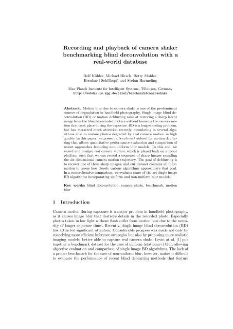
Recording and playback of camera shake: benchmarking blind deconvolution 3Contributions of this paper:1. A new setup for recording and playing back camera shake.2. An extensible benchmark dataset with ground truth data.3. A comprehensive comparison of state-of-the-art single image BD algorithms.3 Recording trajectories of human camera shakeHuman camera shake can be characterized by a six dimensional motion trajectory,with three translational and three rotational coordinates changing throughtime. We decided to measure such trajectories for several subjects holding acompact camera (Samsung WB600), since such cameras are in wide spread use.Typically, they have a small maximum aperture, and images thus get blurredby camera shake if the available light is insufficient and the use of a flash isexcluded. In such cases, an exposure time of 1/3 sec, as used throughout ourexperiments, is realistic.To measure the six dimensional camera trajectory we used a Vicon trackingsystem with 16 high-speed Vicon MX-13 cameras running at a frame rate of500 Hz. The cameras were calibrated to a cube of roughly 2.5m side length.To measure the exact position of the camera during a shake, we connecteda light-weight but rigid construction with markers (reflective balls, size 35mm),see Figure 1. We synchronized the camera shutter with the trajectory data usingthe flash of the camera. As the Vicon cameras are only sensitive to infrared light,the flash light was converted from the optical into the infrared spectrum by usinga photo diode that triggers an infrared lamp.Fig. 1. Setup: (Left) Light-weight structure with reflective spherical markers for recordingcamera shake with a Vicon system. (Right) Camera attached to a high-precisionhexapod robot to take pictures with played back camera shakes in a controlled setting.

4 Recording and playback of camera shake: benchmarking blind deconvolutiondegree0.30.20.10−0.1Rot xRot yRot zRotation of single trajectory−0.20 50 100 150framesmm10.50−0.5Translation of single trajectoryTrans xTrans yTrans z0 50 100 150framesFig. 2. Camera shake: trajectories of the rotation angles (left) and translations (right).Figure 3 depicts the corresponding PSF.Fig. 3. Example of a point spread function (PSF) due to camera shake. Figure 2 showsthe underlying 6D motion in detail. Best viewed on screen rather than in print.

Recording and playback of camera shake: benchmarking blind deconvolution 5Six subjects were asked to take photographs in a natural way. They wereaware that the exposure time was 1/3 sec. 40 trajectories were recorded with thissetup (three subjects with ten trajectories, three subjects with five trajectories;five trajectories had to be excluded due to temporary recording problems). Rawcaptured motion data is noisy in frequency ranges that can not be due to humanmotion. The noise was reduced with an appropriately chosen moving averagefilter. Figure 2 shows example filtered trajectories. Figure 3 shows an exemplarypoint spread function (PSF) obtained by simulating 1 an image of an artificialpoint grid (see Section 5.1 for details).In the next section, we explain how such camera motions can be played backon a robot. This allows us to assess how accurate the motion capture was, andwhether such camera trajectories can be used for a benchmark.4 Playing camera shake on a picture-taking robotThe six dimensional trajectories were played back on a Stewart platform (hexapodrobot, model PI M-840.5PD), which allows minimum incremental motionsof 3µm (x and y axis), 1µm (z axis) and 5µrad (rotations) with a repeatability±2µm (x and y axis), ±1µm (z axis) and ±20µrad (rotations). An SLR camera(Canon Eos 5D Mark II) that can be remote controlled was mounted to theStewart platform to allow synchronization of the camera trigger with the platform(see Figure 1 for the complete setup). For the benchmark dataset (detailedin the following) a printed image was mounted at a distance of 62cm from thecamera.To qualitatively assess whether a real camera shake movement can be recordedand played back by our setup, we took long exposure images of a point grid ofLEDs with a somewhat exaggerated camera shake (to obtain large visible blurs).Simultaneously, we recorded the six dimensional camera trajectory. The recordedtrajectory was played back on the Stewart platform and the attached camerarecorded a long exposure of the same point grid. Figure 4 shows that the realcamera shake (left images) is correctly simulated by the Stewart platform (rightimages). The existing difference in the images is caused by the fact that differentcameras were used for recording and playing back the trajectory and thatthe distance camera to point-grid could not guaranteed to be exactly 62cm atrecording. Nonetheless, in both examples (upper and lower images) the trueimage blurred by camera shake and the image generated by playing back thecamera trajectory are reasonably similar. This shows that our setup is able tocapture the movement of real camera shake and to play it back again.Note that the playback on the Stewart platform was performed in slowermotion (duration 1sec instead of 1/3sec) to increase the smoothness of the movement— stretching time does not change the obtained PSF.Note that we decided against using the point grid of LEDs during the recordingof the human camera trajectories for the benchmark. We found that the small1 A distance of 62cm, focal length of 50mm were assumed.

6 Recording and playback of camera shake: benchmarking blind deconvolution(a) recorded image(b) played backFig. 4. Two examples (first and second row) of an image with camera shake and itscounterpart generated by playing back the camera trajectory on a Stewart platform.motions of real camera shake (where the photographer tries to keep the camerasteady) can not be seen well with the LED point grid. The grid would have tobe positioned rather close to the camera, resulting in an unnatural feeling oftightness, normally not present while taking a photograph.5 Analyzing camera shake trajectories5.1 Is camera shake uniform or non-uniform?Often surprisingly, blind deconvolution algorithms for uniform blur work quitewell on real world camera shake, even though theoretically, the resulting blurshould be non-uniform, i.e. varying across the image. To study this effect withour trajectories we generate a blurred point grid for a given camera trajectory,see Figure 3 for an example.We denote the camera trajectory by a point sequence p 1 , . . . , p T where eachpoint has six dimensions,p t = [θ x , θ y , θ z , x, y, z] T (1)

Recording and playback of camera shake: benchmarking blind deconvolution 7with the last three coordinates being the shifts in mm, the axis positioned indicatedin Figure 1, the first three coordinates being the rotation angle aroundthe indicated axis.Given an image u showing a point grid (14 × 10 equispaced points, size2808 × 1872), we can visualize the point spread function (PSF) of the cameratrajectory by converting each point p t in time into its corresponding homographyH t (assuming distance of 2m for the point grid), assigning p 1 the identitytransformation. Then the resulting blurry image v is the superposition of thetransformed point grids:v =T∑h t (u) (2)t=1where h t (u) is the image u transformed by H t . The local blur kernels of the resultingPSF ξ can be read off the blurry image v. To quantify the non-uniformness(abbreviated NU) of the PSF ξ, we introduce the following measure: given fourlocal blur kernels ξ lr , ξ ur , ξ ll , ξ ul of the lower right, upper right, lower left andupper left corner, we can calculate how similar they are by comparing the lowerleft with the upper right and the upper left with the lower right blur kernel:NU(ξ) = ‖ξ ll − ξ ur ‖ 2 + ‖ξ ul − ξ lr ‖ 2, (3)2where each blur kernel is normalized to have L2-norm one. Note that the differencebetween two blur kernels has to be minimized over all possible shifts(omitted in the formula for clarity). This can be achieved efficiently by notingthat ‖ξ 1 − ξ 2 ‖ 2 = ξ T 1 ξ 1 + ξ T 2 ξ 2 − 2ξ T 1 ξ 2 , where the first summands are one dueto normalization and the inner products for different shifts are the cross correlationsbetween ξ 1 and ξ 2 . Minimizing ‖ξ 1 − ξ 2 ‖ 2 for all possible shifts is thusdone by maximizing the cross-correlation between ξ 1 and ξ 2 .Note that for a perfectly uniform blur (pure shift trajectory along x andz axes), i.e. a camera that has no rotations and no y component, the nonuniformnessindex NU is equal to zero. Figure 5 shows the extreme corners oftwo PSF images generated from recorded camera trajectories. The left exampleis the most uniform blur according to the NU criterion, the right example isthe most non-uniform blur. Also qualitatively, we observe that the NU criterioncaptures non-uniformness. In the middle is the histogram of the NU values of all40 PSFs.5.2 How well can we approximate the 6D trajectory with 3D?To decrease the complexity of possible PSFs, the six dimensional real cameratrajectory is often approximated with three dimensions. There are two mainapproaches:(a) ignore the shifts and model only three rotations (θ x , θ y , θ z ) [2].(b) model only shifts (x and z) and rotation around the visual axis (θ y ) [3, 18],

8 Recording and playback of camera shake: benchmarking blind deconvolutionmost uniform blurmost non-uniform blur.· · ·..· · ·.· · ·NU = 0.68· · ·NU = 1.67Fig. 5. PSF images of recorded camera trajectories being most uniform (left) and mostnon-uniform (right) according to the NU criterion. Histogram of all NU values (middle)..blur 1 blur 2· · · · · ·..· · · · · ·6D (a) (b) 6D (a) (b) 6D (a) (b) 6D (a) (b)Fig. 6. Mapping the 6D camera trajectory to 3D using Whyte et al.’s approach (a) andGupta et al.’s approach (b). Each image patch compares the blur due to the original6D representation to (a) and (b). We set the focal length to 50mm and the objectdistance to 2m..Both approximations achieve good results, as can be seen in Figure 6, so we wouldlike to analyze whether this is in correspondence with our recorded trajectories.To this end, we transform the trajectories to three dimensions following the twoapproaches. Note that the influence of the angles on the shifts and vice versadepends on the distance d of the object to the camera:⎡(a) p t =⎢⎣θ xθ yθ zxyz⎤⎡↦→⎥ ⎢⎦ ⎣0θ y0x − d sin(θ z )0z + d sin(θ x )⎤⎥⎦⎡(b) p t =⎢⎣θ xθ yθ zxyz⎤⎡↦→⎥ ⎢⎦ ⎣θ x − arcsin(x/d)θ yθ z + arcsin(z/d)000⎤⎥⎦Assuming an object distance of d = 2m we transform all 40 camera trajectoriesto three dimensions using mapping (a) and mapping (b). Figure 6 showsbased on two examples that both 3D transformations are qualitatively valid. Forfuture research it might be interesting whether there exists another canonicaltransformation from 6D to 3D which preserves the PSFs.

Recording and playback of camera shake: benchmarking blind deconvolution 96 Benchmark dataset for real-world camera shakes6.1 Recording images with played back camera shakeAs described in Section 4 the image blurs created by the Stewart platform aregood approximations to real image blurs. So we create a benchmark dataset ofimages blurred by camera shake by playing back human camera shakes on thehexapod for different images, see Figure 7.We randomly selected two blur trajectories of each of the six subjects applyingthem to four images (Figure 7) resulting in 48 blurry images. Some localblur kernels turned out rather large. We decided to leave those blur kernels inthe benchmark, as they reflect natural camera shake, probably caused by holdingthe camera too relaxed and not paying attention to hold it still, as couldhappen in real imaging situations. Even though such images are often erased,it is interesting whether current or future deblurring algorithms can cope withsuch large blur kernel sizes.Fig. 7. The four original images used in the benchmark.As discussed in Section 5.1 some of the blurs are approximately uniformand some are not. Eyeballing the generated PSFs (included in the supplementarymaterial), the blur kernels numbered 1,3,4,5,8,9,11 (see table 1) tend tobe approximately uniform, while blur kernels 2,6,7,10,12 appear non-uniform, inaccordance with the NU criterion. Kernels 8 and 11, although having a high NUvalue still visually appear to be uniform. The non-uniformness detected by theNU value is not clearly visible due to the large size of the kernels.For recording the image database, the Steward platform was placed inside alight-tight box. The SLR camera was set to ISO 100, aperture f/9.0, exposuretime 1sec, taking images in the Canon raw format SRAW2. A Canon EF 50mmf/1.4 lens was used. The illumination inside the box was adjusted to the cameraparameters and kept constant for all images taken. The true sharp image wasmounted as a poster at a distance of 62cm to the camera. The complete setupis shown in Figure 1.The recorded SRAW2 images (16bit) were processed by DCRAW 2 , generating8bit images without correcting gamma. From the center of the image, a2 DCRAW was called with parameters -W -g 1 1 -r 1.802933 1.0 2.050412 1.0 -b 4)

10 Recording and playback of camera shake: benchmarking blind deconvolution800 × 800 patch was cropped. The blurry images are named (i, j) for the i-thimage blurred with the j-th camera trajectory.6.2 Recording ground truth imagesEven though the original images are available since we printed them onto posters,comparing these images with deblurred images from some algorithm is not easy,because of different image resolution, different lighting, and possible color differencesdue to the printing process. Instead our robotic setup allows us to generateground truth images along the trajectory by playing the camera trajectory stepby step and taking an image per step.Using this strategy, we recorded for each of the 48 blurry images (12 camerashakes each blurring 4 images) 167 images along the trajectory. Additionally, wecreated 30 images at intermediate positions calculated by the hexapod duringplayback. We denote the ground truth images by u ∗ 1, . . . , u ∗ N .6.3 Measuring the deblurring performanceTo compare similarity between two images a and b (represented as vectors), wefirst estimate the optimal scaling ˆα and translation ˆT such that the L2 normbetween a and b becomes minimal 3 , i.e. ˆα, ˆT = min α,T ‖a − T (αb)‖ 2 . We thencalculate the peak-signal-to-noise ratio (PSNR) asPSNR(a, b) = 10 log 10m 2〈‖a i − ˆT (ˆαb i )‖ 2 〉 i(4)with 〈.〉 i denoting an average over pixels and m being the maximal possibleintensity value, i.e. m = 255 as we work with 8bit encoding. Given a sequenceof ground truth images u ∗ 1, . . . , u ∗ N along the trajectory, we define the PSNRsimilarity between an estimated image û and the ground truth as the maximumPSNR between û and any of the images along the trajectory,SIM = maxn PSNR(u∗ n, û). (5)7 Comparing state-of-the-art algorithms in motiondeblurringIn the following comparative evaluation, we present the results of current stateof-the-artalgorithms in single image BD on our benchmark dataset. The algorithmscan be divided into two groups:– Algorithms which assume a uniform blur model and account for translationalmotion only [7, 10–13].3 We allow for integer pixel translations only, which we estimate with the Matlabfunction dftregistration by [24]

Recording and playback of camera shake: benchmarking blind deconvolution 11– Algorithms which assume a non-uniform blur model. In particular, [2, 19]assumes rotational motion (yaw, pitch and roll), while [18] considers translationsand in-plane rotations only.For fair comparison, we asked the authors of the tested algorithms to runtheir code on our benchmark dataset and to provide us with their best deblurringresults. The results reported for [10, 12, 18, 19] were provided by the authors,while for [7, 11, 13] we used provided code to yield the deblurring results ourselves.Regarding parameter settings, we followed the provided instructions orthe personal advice of the authors and did our best to optimally adjust thefree deblurring parameters incl. kernel size (and image patch in the case of [7]).Table 1 reports the PSNR for all of the 48 benchmark images, where we computedthe PSNR according to Eq. (5) as detailed in the previous section. Forbetter visual assessment we color coded the results from blue (low PSNR, poorperformance), green (intermediate PSNR) to red (high PSNR, good deblurringperformance). All deblurred images incl. the estimated kernels are shown in thesupplementary material.Insights:– Not all deblurring algorithms are able to improve image quality, which isdue to artifacts which arise during the deblurring process.– Overall performance is content specific as evident by the horizontal bandstructure in Table 1. In particular, image motives 1 and 3 yield consistentlybetter deblurring results.– All except for the methods of [11, 12] have difficulties with large blur (kernel8-11).– The algorithm of Xu et al. [12], which features a robust two-phase kernelprocedure, performs best despite its assumption of a uniform blur model,followed by the recently proposed algorithm of Whyte et al. [19] which allowsfor non-uniform blur.– More recently proposed algorithms yield a better overall performance, beingevidence of the progress in the field.Although runtime is a critical factor and a discriminantive feature of deblurringalgorithms, we do not report any runtimes here as the results were obtainedby heterogenous implementations (e.g. Matlab vs. C) and different hardwaresystems (e.g. CPU vs. GPU).8 Discussion and ConclusionIn this paper, we presented a new benchmark dataset for evaluating single imageBD algorithms. To this end we first recorded and analysed real camera shakeand investigated how well currently employed imaging models approximate andcapture true motion blur. To mimick real camera shake we employed a robot platformfeaturing six degrees of freedom and therefore fully capable of replaying the

Recording and playback of camera shake: benchmarking blind deconvolution 13recorded camera trajectories, while at the same time providing the opportunityto sample the true camera motion trajectory with steady image captures to yielda sequence of ground truth images.The benchmark has been designed to be extendable. In ongoing work wefurther investigate the limitations of current approaches by adding complexityto the imaged scenes such as varying depth. We intend to extend our benchmarkfor new sets of images and camera shakes where current methods fail to givesatisfactory results. At the same time we examine other quality measures thanPSNR, some of which hold the promise to better resemble human perception.Another interesting future direction is to study whether users exhibit repeatingcamera shake patterns. Such a finding would motivate to learn personalizedpriors which ultimately could facilitate BD.The benchmark dataset is publicly available at the accompanying projectwebpage 4 . We hope that it will find widespread acceptance within the communityas a useful tool to evaluate the performance of new BD algorithms, rendering ita valuable resource for monitoring the state-of-the-art in the field.References1. Levin, A., Weiss, Y., Durand, F., Freeman, W.T.: Understanding and evaluatingblind deconvolution algorithms. In: Proceedings of the IEEE Conference onComputer Vision and Pattern Recognition (CVPR). (2009)2. Whyte, O., Sivic, J., Zisserman, A., Ponce, J.: Non-uniform deblurring for shakenimages. In: Proceedings of the IEEE Conference on Computer Vision and PatternRecognition (CVPR). (2010)3. Gupta, A., Joshi, N., Zitnick, C.L., Cohen, M., Curless, B.: Single image deblurringusing motion density functions. In: Proceedings of the European Conference onComputer Vision (ECCV). (2010)4. Richardson, W.H.: Bayesian-based iterative method of image restoration. Journalof the Optical Society of America 62 (1972) 55–595. Lucy, L.B.: An iterative technique for the rectification of observed distributions.The Astronomical Journal 79 (1974) 745–7546. Kundur, D., Hatzinakos, D.: Blind image deconvolution. Signal Processing Magazine13 (1996) 43–647. Fergus, R., Singh, B., Hertzmann, A., Roweis, S.T., Freeman, W.T.: Removingcamera shake from a single photograph. In: ACM Transactions on Graphics (SIG-GRAPH). (2006)8. Miskin, J., MacKay, D.J.C.: Ensemble learning for blind image separation anddeconvolution. In: Advances Independent Component Analysis. (2000)9. Field, D.J.: What is the goal of sensory coding? Neural computation 6 (1994)559–60110. Shan, Q., Jia, J., Agarwala, A.: High-quality motion deblurring from a singleimage. In: ACM Transactions on Graphics (SIGGRAPH). (2008)11. Cho, S., Lee, S.: Fast motion deblurring. In: ACM Transactions on Graphics(SIGGRAPH ASIA). (2009)4 http://webdav.is.mpg.de/pixel/benchmark4camerashake

14 Recording and playback of camera shake: benchmarking blind deconvolution12. Xu, L., Jia, J.: Two-phase kernel estimation for robust motion deblurring. In:Proceedings of the European Conference on Computer Vision (ECCV). (2010)13. Krishnan, D., Tay, T., Fergus, R.: Blind deconvolution using a normalized sparsitymeasure. In: Proceedings of the IEEE Conference on Computer Vision and PatternRecognition (CVPR). (2011)14. Levin, A., Weiss, Y., Durand, F., Freeman, W.T.: Efficient marginal likelihoodoptimization in blind deconvolution. In: Proceedings of the IEEE Conference onComputer Vision and Pattern Recognition (CVPR). (2011)15. Tai, Y.W., Tan, P., Brown, M.S.: Richardson-lucy deblurring for scenes under aprojective motion path. Technical Report of Korea Advanced Institue of Scienceand Technology (KAIST) (2009)16. Tai, Y.W., Tan, P., Brown, M.S.: Richardson-lucy deblurring for scenes undera projective motion path. IEEE Transactions on Pattern Analysis and MachineIntelligence (PAMI) (2011)17. Harmeling, S., Hirsch, M., Schölkopf, B.: Space-variant single-image blind deconvolutionfor removing camera shake. In: Advances in Neural Information ProcessingSystems (NIPS). (2010)18. Hirsch, M., Schuler, C.J., Harmeling, S., Schölkopf, B.: Fast removal of non-uniformcamera-shake. In: Proceedings of the IEEE International Conference on ComputerVision (ICCV). (2011)19. Whyte, O., Sivic, J., Zisserman, A.: Deblurring shaken and partially saturatedimages. In: Proceedings of the IEEE Workshop on Color and Photometry in ComputerVision, with ICCV 2011. (2011)20. Yuan, L., Sun, J., Quan, L., Shum, H.Y.: Image deblurring with blurred/noisyimage pairs. In: ACM Transactions on Graphics (SIGGRAPH). (2008)21. Raskar, R., Agrawal, A., Tumblin, J.: Coded exposure photography: motion deblurringusing fluttered shutter. In: ACM Transactions on Graphics (SIGGRAPH).(2006)22. Cho, T.S., Levin, A., Durand, F., Freeman, W.T.: Motion blur removal with orthogonalparabolic exposures. In: IEEE International Conference in ComputationalPhotography (ICCP). (2010)23. Joshi, N., Kang, S.B., Zitnick, C.L., Szeliski, R.: Image deblurring using inertialmeasurement sensors. In: ACM Transactions on Graphics (SIGGRAPH). (2010)24. Guizar-Sicairos, M., Thurman, S.T., Fienup, J.R.: Efficient subpixel image registrationalgorithms. Optical Letters 33 (2008) 156–158