Solar Wind Magnetosphere Coupling
Solar Wind Magnetosphere Coupling
Solar Wind Magnetosphere Coupling

You also want an ePaper? Increase the reach of your titles
YUMPU automatically turns print PDFs into web optimized ePapers that Google loves.
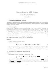
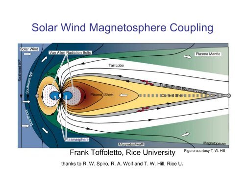
<strong>Solar</strong> <strong>Wind</strong> <strong>Magnetosphere</strong> <strong>Coupling</strong>Frank Toffoletto, Rice Universitythanks to R. W. Spiro, R. A. Wolf and T. W. Hill, Rice U.Figure courtesy T. W. Hill
Outline• Introduction• Properties of the <strong>Solar</strong> <strong>Wind</strong> Near Earth• The Magnetosheath• The Magnetopause• Basic Physical Processes that control <strong>Solar</strong><strong>Wind</strong> <strong>Magnetosphere</strong> <strong>Coupling</strong>– Open and Closed <strong>Magnetosphere</strong> Processes– Electrodynamic coupling– Mass, Momentum and Energy coupling– The role of the ionosphere• Global MHD codes at CCMC• Current Status and Summary
Introduction• By virtue of our proximity, the Earth’smagnetosphere is the most studied and bestunderstood magnetosphere– However, the system is rather complex in itsstructure and behavior and there are still somebasic unresolved questions– Today’s lecture will focus on describing thecoupling to the major driver of the magnetosphere- The solar wind, and the ionosphere
Figure courtesy NASAThe <strong>Solar</strong> <strong>Wind</strong> Near the Earth
<strong>Solar</strong>-<strong>Wind</strong> Properties Observed Near Earth• <strong>Solar</strong> wind parameters observed by many spacecraftover period 1963-86. From Hapgood et al. (Planet.Space Sci., 39, 410, 1991).
<strong>Solar</strong> <strong>Wind</strong> Observed Near EarthParameter Mean σ Median 5-95%range limitNumberDensity (cm -3 )Observedmin andmax values8.7 6.6 6.9 3-20 0.1-83Velocity (km/s) 468 116 442 30-270 250-2000Ram Pressureρv 2 (nPa)7 5.2 5.5 0.01-14.5 0.05-28Magnetic Field(nT)Ion Temp.(10 5 K)ElectronTemp. (10 5 K)6.2 2.9 5.6 2.2-9.9 0-851.2 0.9 1.0 0.1-3 0.1-31.4 0.4 1.3 0.9-2 1-2From Feldman et al. (<strong>Solar</strong> Output and its Variations, Colorado Assoc. Univ. Press, 1977)
<strong>Solar</strong> <strong>Wind</strong> Observed Near EarthΔB z ΔB y • Observed near Earth, the interplanetary magneticfield tends to make ~ 45˚ or ~225˚ angle with Sun-Earth direction.– Parker spiral.• The north-south component of the IMF averages nearzero and fluctuates on short time scales
<strong>Solar</strong>-Cycle Variation of <strong>Solar</strong> <strong>Wind</strong> Near EarthFrom Hapgood et al.(1991) • Average velocity highest in declining phase of solarcycle.• Successive solar cycles represent different polaritiesof Sun’s magnetic field.• Magnetic-field reversal occurs near solar maximum.
<strong>Solar</strong>-Cycle Variation of <strong>Solar</strong> <strong>Wind</strong> Near Earth• Plot shows average absolute value of northsouthIMF component.• Highest near solar maximum.
• The energy of the solar wind has 3components:– Thermal– Magnetic– Flow• Which has the largest energy density?
Magnetosheath– Gasdynamic Aspects• The energy of the solar wind is dominated by the flow• The theoretical way to deal with this is to treat theflow as gasdynamic and to neglect the magnetic field.– Back in the 1960’s, John Spreiter and colleagues convertedan existing numerical code to describe the bow shock andmagnetosheath. The code had been developed to treat theflow around missiles.– They assumed an axially symmetric shape for themagnetopause.• Since the solar wind is supersonic, it forms a shockas it encounters the Earth’s magnetosphere andslows down– The collision mean free path of the solar wind is of the orderof ~10 6 R E , the thickness of the bow shock is of the order ofthe ion gyroradius (~1000 km)
Density Distribution• Density:– For Mach number 8 and γ = 5/3, the model calculationindicates that the density jumps by a factor 3.82 across theshock.– Max density is at “subsolar point,” 4.23 times solar winddensity.– Density gradually decreases away from subsolar point.
Velocity and TemperatureDistributions• Temperature decreases away from subsolarpoint• Velocity increases away from that point.• The contours for T and v are the same.
Magnetic Field DistributionB ^ vB at 45˚ to v• Computed from assumption of frozen-in flux• Note how magnetic field lines hang up on nose ofmagnetosphere• B highest near subsolar point.– Zwan-Wolf effect• In reality, the magnetosheath is very noisy
Effects of Mach Number
Magnetic Cloud Events• Most very large magnetic storms on Earth are causedby magnetic clouds or “islands.”– Strong organized magnetic field– Long period of northward field and long period of southwardfield.• Southward field causes storm
Magnetopause formationSnapshot from the LFM global magnetosphere code
Definition of “Magnetopause”• An observer would want to define it in terms ofsomething that is easy to observe, like a sharp jumpin ‘something’.• A theorist would want to define it in profoundtheoretical terms, such as the boundary betweenopen and closed field lines.– However, that theorist’s definition doesn’t work - isn’tconsistent with the established definition of themagnetosphere, which is the region dominated by Earth’smagnetic field.– Polar caps lie on open field lines, but at low altitudes theycertainly lie in a region dominated by Earth’s field.• We use an observational definition--a sharp changein the magnetic field.
Chapman-Ferraro-Type Magnetopause• Solution for the magnetic field:0.8BB m.0.60.40.2-2-101 2 3 4 5y/d• The B-field scale length isa cm = mv relatedo= d to the gyroradius inside themagnetosphere:qB m 2• The momentum/area/time that the particles impart to themagnetic boundary is22 B2n o mv o = m2µ o– Intuitively reasonable• The most fundamental conclusion of Chapman and Ferrarowas that a boundary would form between the solar windand magnetosphere, and that the solar wind wouldbasically not penetrate to the space near Earth.
Chapman-Ferraro-Type Magnetopauseyzx• One problem: charge imbalance:– <strong>Solar</strong> wind electrons presumably have the same density and flowvelocity as the ions.– The electrons are much easier to turn around than the moremassive ions– There is a negative charge layer above the positive charge layer– Order-of-magnitude estimate:Surface charge density = σ c ~ n o qd– Potential difference across the charge separation layer:ΔV ~ σ c d m~ iε o 2µ o ε o q ~ m i c22qB~ 500 × 106 V
Chapman-Ferraro-Type MagnetopauseyzxB• Such a large potential drop can’t be driven by particles ~ 1 keV• Chapman and Ferraro realized this, and they enforced quasineutralityand calculated a self-consistent electric field.– They calculated a potential drop ~ mv o2 /2• Parker later pointed out that the magnetopause field linesconnect to the conducting ionosphere.– If the charge density were maintained for a substantial time, thencharges would flow up to and from the ionosphere, to eliminate thecharge imbalance.
Models with a Self-ConsistentlyComputed Magnetopause• The first models with a self-consistently computed magnetopause weredeveloped in the early 1960’s.• AssumeB o = 0where “o” means outside the magnetopause. Since, ∇⋅ B = 0werequireB i ⋅n ˆ = 0The total pressure in the magnetosheath just outside themagnetopause is estimated from the formulap o = kρ sw ( n ˆ ⋅v sw ) 2k=2 corresponds to the Chapman-Ferraro model. k=1 corresponds toparticles sticking to the boundary. k=0.884 corresponds to thegasdynamic model with γ=5/3, M=8.• The field just inside the magnetopause satisfies the pressure balancerelation2n ˆ × B i= kρ2µ sw (ˆ n ⋅ v sw ) 2o
Models with a Self-ConsistentlyComputed MagnetopauseMead (1964) model• This model has a self-consistently computed magnetopause– No magnetotail (wasn’t discovered until 1965)– Assumed ∇ × B = 0 inside the magnetopause.
Question• In what direction is the magnetic fieldassociated with the Chapman Ferrarocurrents?
Magnetospheric Current Systems
Early Self-Consistently ComputedMagnetopauses3 versions of Choe/Beard/Sullivanmodel in noon-midnight plane.[Q: Why is there an indentation?]Model equatorial cross section
Dependence of Standoff Distance on<strong>Solar</strong>-<strong>Wind</strong> Parameters• DefineB subsolar subsolari= 2 f B dipole• The real magnetopause is between these two extremes.• The results of the problem suggest that1.0 ≤ f ≤ 1.5• The pressure-balance relation becomes⎡2 1 ⎛kρ sw v sw =⎢ R2 fB E2 o µ ⎢ ⎜ o ⎣ ⎝ r so• Solving for r so gives⎛2 f 2 2B⎞r so = R ⎜ o ⎟E ⎜ 2⎝ kµ o ρ sw v⎟ sw ⎠1/ 6⎞ 3⎤2⎥⎟⎠⎥⎦= 11.43 R E2ρ sw v sw1/ 6( ) nPa⎛ f ⎞1/ 3 ⎛ 0.885 ⎞⎜ ⎟ ⎜ ⎟⎝ 1.16⎠⎝ k ⎠The best-estimate value for f is about 1.16 . A nominal solar wind (5cm -3 , 400 km/s) corresponds to ρ sw v sw2= 1.34 nPa, which correspondsto r so =10.91/ 6
Empirical Magnetopause ShapesAverage observed shape of magnetopause. Solid curve is -5 nT, dotted curve -2.5nT, dashed curve 0, dash-dot 2.5 nT, dash-dot-dotdot5.0 nT. Adapted from Roelof and Sibeck (JGR, 99, 8787, 1994)• Note– Southward IMF moves magnetopause closer to Earth, strengthens taillobes.• Magnetopause position doesn’t vary over a wide range (1/6 th power)– Subsolar standoff distance is nearly always between 6.6 R E and 14 R E .
Features of the ObservedMagnetic Field-DBSugiura and Poros plot of average DB for Kp=0 or 1.• Obvious features:ΔB = B observed– Compression of day side– Enhanced field in tail lobes– Depression in polar cusp− B dipole– Depression of field near Earth and equatorial plane due to ringcurrent
Decline of B Z Downtail• For x > -20,– B z is nearly always positive on the flanks of the tail,occasionally negative near local midnight– The B z distributions are much broader (indicating morevariability)• Suggests both occasional x-lines earthward of -20.• Consistent with dipolarization of field in expansion phase.• For -45< x < - 20,– | B z | smaller.– Sector doesn’t matter much.
B z Further DowntailHistograms of z component of B in plasma sheet, fromISEE-3. From Siscoe et al.(1984).• 60-80 R E behind Earth, B z is still usually positive.• 225 R E behind Earth, B z is negative more than halfthe time.
Where Does Average B z TurnNegative?Location of separatrix between interplanetary field liensand closed field lines, from Slavin et al. (1985).• Neutral line of average B z :– ~ 130 R E near local midnight– ~ 300 R E on the flanks• The “wake”, which consists of field lines that areconnected to the interplanetary medium on both“ends”, becomes a larger and larger part of the tailas you go downstream.
<strong>Coupling</strong> processes
Basic MagnetosphericConvection• <strong>Solar</strong> <strong>Wind</strong> <strong>Magnetosphere</strong> <strong>Coupling</strong>produces a system of plasma convection– Plasma in to the high latitude region connected tothe outermost layers of the magnetosphere flowanti-sunward– Plasma in to the low latitude connected to theinner magnetosphere generally flow sunward– The presence of such convection suggest someform of drag or frictional force acting across themagnetopause
Polar-Cap Potential DropABEEquipotentialsand flow lines• The potential drop across the high-latitude ionosphere can bemeasured by a polar-orbiting spacecraft.Φ pcp =B∫AE⋅dl– The polar cap potential drop F pcp is measured routinely bysatellites traversing the high-latitude ionosphere.
Polar-Cap Potential DropABEEquipotentialsand flow lines• Technical Problem: Satellite track doesn’t usually cross eitherthe max potential point A or the minimum potential point B.– Difference between max and min potential on satellite track is alower limit on F pcp .– Use only spacecraft in dawn-dusk orbit and estimate correction.– DMSP ion drift meter makes routine measurements of velocityperpendicular to the spacecraft track.• Observed values:20 kV ≤ Φ pcp ≤ 250 kVΦ pcp≈ 50 kV
Polar-Cap Potential Drop Driven by ViscousInteraction(adapted from Hill, 1983)• Originally suggested by Axford and Hines (1961).• Assume that the field lines are approximately equipotentials.• If the average observed polar cap potential (50 keV)h B v ⊥~ 25 kVIf= 30 nT and =150 km/s (slightly less than half thesolar-wind speed),h ~ 6000 kmAre there closed-model processes strong enough to createa closed-field-line boundary layer ~ 1 R E thick?
Kelvin-Helmholtz Instability(Miura, 1984)• Kelvin-Helmholtz instability is driven by a velocity shear– Ideal-MHD instability– Causes crinkling of the boundary– Velocity swirls– Tends to be stabilized by different magnetic field directions on thesides of the shear– In nonlinear phase, causes macroscopic friction– Computer simulations suggest 10-30 kV potential drop acrossmagnetosphere (maybe enough to explain quiet-time convection)
Gradient/Curvature Drift ThroughMagnetopause• The scale length L parallel to the boundary is~10R E .• To form a boundary 1 R E thick about 20 R E behindEarth, the average gradient-drift speed would have tobe at least /20, and ~v^. Therefore, theratio in is too small by almost 2 orders of magnitude.• Conclusion: Gradient drift doesn’t transport particlesfast enough drive observed convection underaverage conditions.
Wave-Induced Diffusion Across theMagnetopause• The magnetosheath has a lot of electromagnetic noise. Maybethat jiggles charged particles across field lines to form a thickboundary layer.• Bohm diffusion (treatment from Hill, 1983):– To get an idea of how fast such wave-induced diffusioncould possibly be, picture each wave-particle interaction as acollision. Assume the particle’s velocity is completelyrandomized after each collision.– For the magnetopause boundary layer, put kT=200 eV, B=20 nT,and get a diffusion coefficientΔx 2 ~ 2 × 600 × 1200 ~ 1200km• This is ~ one-fifth the boundary-layer thickness required to drivethe average observed convection.
Summary - closed transfer processes• Optimistic estimate of Kelvin-Helmholtz provides
Low-Latitude Boundary LayerPlasma SheetVan Allen Belts(Radiation Belts)SubsolarPointPlasmapausePlasmasphereLow-LatitudeBoundary Layer<strong>Solar</strong> <strong>Wind</strong>Magnetosheath• Conventional wisdom is that much of the observed low-latitudeboundary layer, which consists of antisunward-flowing plasmaon the magnetopause, on northward-pointing magnetic fields, isdriven by these closed-field-line transfer processes.• These processes operate, but are not the primary drivers ofconvection.
Magnetic Reconnection• Magnetic reconnection is the process wherebyplasma ExB drifts across a magnetic separatrix, i.e.,a surface that separates regions containingtopologically different magnetic field lines– (Vasyliunas, Rev. Geophys. Space Phys., 13, 303, 1975)– In the original Dungey picture, reconnection occurs both onthe dayside magnetopause and in the magnetotail.
Empirical evidence• Correlation ofpolar-cap potentialdrop with VB z(From Reiff andLuhmann (1986))
Summary - Open<strong>Magnetosphere</strong>• The open model of the magnetosphere(Dungey, 1961) implied that convection wouldbe strong for southward IMF– IMF is roughly anti-parallel to Earth’s dipole– Facilitates reconnection at dayside magnetopause• That basic prediction has been stronglyconfirmed.• This was substantial evidence thatreconnection at the dayside magnetopausewas the dominant driver of magnetosphericconvection.
Polar Cap Saturation (Predicted by Hill, confirmedby simulations)
Effect of IonosphericConductance• The ionosphere plays an important role on determiningthe rate of convection on the ionosphere• The larger the conductance, the lower the convectionrate
Where Does Average B z Turn Negative?Location of separatrix between interplanetary field liensand closed field lines, from Slavin et al. (1985).• Neutral line of average B z :– ~ 130 R E near local midnight– ~ 300 R E on the flanks• The “wake”, which consists of field lines that areconnected to the interplanetary medium on both“ends”, becomes a larger and larger part of the tailas you go downstream.
Transfer of Particles into the Closed-Field-Line Region of the <strong>Magnetosphere</strong>• Rate of earthward ion convection in thepl.sh.plasma sheet: Φ ions ~ (1cm−3 )(50km / s)(8RE )(30 R E ) ~ 5×10 26 s −1• <strong>Solar</strong>-wind particles incident on the front ofthe magnetosphere: Φ ions• Efficiency of particle penetration, assuminghalf the plasma sheet comes from the solarpl.sh.Φwind: η ions ~ ions2Φ ionssolar wind ~ (5cm−3 )(400km / s)π(15RE ) 2 ~ 6 ×10 28 s −1solar wind ~ 0.004
Question• Roughly what is the total amount ofmass in the magnetosphere?– 2x10 20 tons– 2x10 10 tons– 20 tons– 2x10 -12 tons
Transfer of Energy into the Inner<strong>Magnetosphere</strong>/Ionosphere• Rate of Joule dissipation in the ionosphere:Joule heat ~ (2 hemispheres)(50, 000volts )(106 A) = 1011 wattsΦ energy• Estimated total dissipation in inner magnetosphere andionosphere:diss.Φ energy~ 2 ×10 11 watts• Energy flux of solar wind times cross section of magnetosphere:swΦ energy⎛~ n sw m i v sw3 ⎞⎜ ⎟⎜⎝ 2 ⎟ π 15R E⎠( ) 2 ≈ (5cm−3 )2m H (400km / s) 3 π 15R E( ) 2 ~ 8 ×10 12 watts• Efficiency with which energy penetrates to the magnetosphericinterior and ionosphere:η energy = Φ dissipationenergy~ 0.025swΦ enery
Transfer Efficiencies for Fluid Quantities• Much more mass enters the plasma mantle andimmediately escapes down the tail. That masswasn’t counted in the efficiency.• Much more energy also enters the magnetosphere inthe plasma mantle and escapes down the tail butwasn’t counted in the efficiency. The loss of solarwind kinetic energy is estimated assw to tailΦ energy~ (B lobe) 2µ o(v sw)π(R tail) 2 / 2~ (20 × 10−9 nT ) 2µ o(4 × 10 5 m / s)π(15 × 6.37 × 10 6 m) 2 / 2 ~ 3 × 10 12 wattswhich is much larger than the energy dissipated in theionosphere and magnetospheric interior.
Energy Input - Poynting Flux• It can be shown that the rate of conversion to/from mechanical energy from/to magneticenergy is given by (Hill, 1982)< j.E >= − < ∇i(E × B) / µ 0>• Where < > is a (sufficiently) long time average• Basically, when– j.E > 0, magnetic energy is converted to flowenergy– j.E < 0 flow energy is converted to magneticenergy
Example from Global MHD -Southward IMFSWMFX(Re)-40-30-20-1001020Y(Re)-30-20-100102030Z(Re)-30-20-100102030E.J(pW/m^3)21.61.20.80.40-0.4-0.8-1.2-1.6-2BATSRUSIMF Bz=-6nTLFMX-40-30-20-1001020Y-30-20-100102030Z-30-20-100102030E.J(pW/m^3)21.61.20.80.40-0.4-0.8-1.2-1.6-2LFMIMF Bz=-5nT
Example from Global MHD –Northward IMFSWMFLFMX(Re)-40-30-20-1001020Y(Re)-30-20-100102030Z(Re)-30-20-100102030E.J(pW/m^3)21.61.20.80.40-0.4-0.8-1.2-1.6-2BATSRUSIMF Bz=5nTX-40-30-20-1001020Y-30-20-100102030Z-30-20-100102030E.J(pW/m^3)21.61.20.80.40-0.4-0.8-1.2-1.6-2LFMIMF Bz=5nT
Momentum <strong>Coupling</strong>• How does the force applied by solarwind manifest itself in themagnetosphere?– At the magnetopause, both normal andtangential forces are acting– The normal force is the solar wind rampressure isRam force ~ ram pressure × area presented to the SW (5 cm −3 )(1.67 × 10 −27 kg)(400 km / s) 2 π(15R E) 2~ 4 × 10 7 N
Question• Which is larger?– <strong>Solar</strong> wind dynamic pressure?– <strong>Solar</strong> radiation pressure?
Question• Which is larger– <strong>Solar</strong> wind dynamic pressure? ~2x10 -9 Pa– <strong>Solar</strong> radiation pressure? ~5x10 -6 Pa
Question• Which is larger– <strong>Solar</strong> wind dynamic force?– <strong>Solar</strong> radiation force?
Question• Which is larger– <strong>Solar</strong> wind dynamic force? ~2x10 7 N– <strong>Solar</strong> radiation force? ~6x10 8 N
Comment on Forces• With a force ~10 7 N, the ~200+ tons ofplasma in the magnetosphere would beblown down the tail• Ultimately the only mass able to hold offthe force is the Earth itself [Vasyliunas,2007]
Force of Chapman-FerraroCurrent on the dipoleF CF≈ µ.∇B CF≈ (8 × 10 22 )(1.5nT / R E)≈ 2 × 10 7 NMidgley and Davis, 1963) From Siscoe and Siebert, JASTP 2006
Siscoe and Siebert,2006 got 2.4x10 7 N byintegrating themomentum stresstensor over the volume. From Global MHDFrom Siscoe and Siebert, JASTP 2006
Changes of Chapman Ferraroand R-1 currents withincreasing IMF Ey.From Siscoe and Siebert, JASTP 2006
ForceTan=positive, blue=negativeFrom Siscoe and Siebert, JASTP 2006
Tailward force on the thermosphereexceeds solar wind dragThis was also noted by Hill, 1982 and discussed in detail by Vasyliunas, 2007From Siscoe and Siebert, JASTP 2006
Comments on Transfer Efficienciesfor Fluid Quantities• Efficiency of momentum transfer:(20 nT) 2DragRam force ~ 2µ o(5 cm −3 )(1.67 ×10 −27 kg)( 400 km/ s) 2 ~ 0.12where the numerator is an estimate ofthe tension force per unit area on thetail.
Penetration of <strong>Solar</strong>-<strong>Wind</strong> Magnetic• Magnetic flux:Flux into Magnetotail– The magnetic flux in the polar cap (or tail lobes) is estimated aspc ⎛ 15° ⎞ 2Φ Bn ~ π ⎜ ⎟ (6.27×10 6 m) 2 (. 5×10 −4 T ) ~ 4.4 ×10 8 Wb⎝ 57.296° ⎠These magnetospheric field lines are all connected to thesolar wind and thus represent the effects of reconnection.– The magnetic flux that would thread through the regionoccupied by the magnetotail, if the magnetotail weren’t thereis estimated as Φsw 6 2 −9 9Bn ~ 40 × 30 × 300 × (6.37 ×10 m) × (5 ×10 T ) ~ 2.4 ×10 Wbso the the efficiency with which the magnetic field getsacross the tail magnetopause is estimated asη Bn ~ Φ pcBnswΦ ~ 0.18Bn
Penetration of E y into<strong>Magnetosphere</strong> in Times ofSouthward IMF• The average observed polar cap potential drop intimes of southward IMF is given roughly byswΦ EtanpcΦ Ey ~ 80kV• The average potential drop across a distance of 30R E (diameter of dayside magnetopause) would be~ vsw B sw (30 R E ) ~ (400 km/ s)(5 nT)(30 × 6.37 ×10 6 ) ~ 382, 000VThe implied efficiency isη Etan = Φ pcEtanswΦ Etan~ 0.21
Summary Comments onEfficiency• Only a small fraction (~1%) of the total particles andenergy incident on the dayside magnetopause getsinto the inner and middle magnetosphere, wherethere is sunward convection.• A much larger fraction of the solar wind particles andmomentum convect through the plasma mantle butnever get deeply involved in the life of themagnetosphere.• About 10-20% of the solar wind electric fieldpenetrates, in times of southward IMF.
Global MHD models• Global MHD models are now able toreproduce many of the global quantitiesdiscussed above• However they often don’t get the exact sameresults for the same inputs– Probably due to numerics such as resolution,numerical methods, etc• While they seem to do a good job getting thegross scale physics correct, there is a lot ofmissing physics in the models– e.g, microphysics of reconnection, drift physics,etc– There has been efforts in the past few years toincorporate missing physics in the models
Essential requirements tosuccessful MHD Modeling• Requirements include– Accurate solution of the MHD equations• Quite difficult, due to the nature of the MHD equations– That said, it is the violation of the ideal MHD requirement that drives the system• Keeping divergence of B requires special techniques– Accurate modeling of the bow shock and boundaries such as themagnetopause– Proper representation of the boundary conditions• Outer boundary is placed in the supersonic regime to eliminate any artifacts• Inner boundary, near the Earth should represent the effects of coupling tothe ionosphere which requires an ionospheric model– Challenges in regions where wave speed get very large (effectsmodel timestep)• Near the Earth, where the magnetic field gets large• In the lobes, where the density is low
Global MHD Models at CCMCModelWhenDevelopedLFM/CMIT mid 80’s StretchedPolarOpenGGCMmid 90’sGrid Institution NumericalMethodStretchedCartesianSWMF late 90’s Cartesianusing AMRCISMUNHCSEMPartialInterfacemethodHybridHartenmethodGodunovmethodDivergence of BYee gridYee gridVarious,includingadvection
MHD Equations (from Lyon et al,∂(ρ v)∂t∂ρ∂t + ∇⋅(ρ v) = 02004)+ ∇⋅[ρ v v + I(P + B22µ 0) −B Bµ 0] = 0∂E∂t + ∇⋅[ v( ρv22 + γγ −1 P)]+ v ⋅∇⋅[I B22µ 0−∂ B∂t − ∇ × ( v × B) = 0E = ρv22 + 1γ −1 P∇⋅ B = 0B Bµ 0] = 0
LFM Grid – Stretched PolarGrid
OpenGGCM Grid
SWMF Grid (from CCMCwebsite)
Magnetosheath comparison
IMFB z =-5nT
IMFB z =-5nT
12121818J II0(a)120(c)---6 18+-++- -DOWNWARD CURRENT0UPWARD CURRENT(b)126 180jhorizontal(d)Ev66
IMF B z =5nT
IMF B z =5nT
Final Comment: we think we understand a lot,but there are still a lot of fundamentalunanswered questions, for example:• To what extent is space weather (like surfaceweather) predictable, and to what extent is it (likesurface weather) inherently unpredictable?• Why are superthermal particles ubiquitous in spaceplasmas?• Most of the solar system is occupied by collisionlessplasma. Why are the positive ions, wherever youlook, about 5-10 times hotter than the electrons?• What is role of kinetic-scale processes in determiningthe large-scale structure of plasmas.?
Thanks!