Transportation Statistics Annual Report1997 - BTS - U.S. ...

Transportation StatisticsO▼Annual Report 1997US DEPARTMENT OF TRANSPORTATIONBUREAU OF TRANSPORTATION STATISTICSmobilityandaccess▼

All material contained in this report is in the public domain andmay be used and reprinted without special permission; citation asto source is required.Recommended citationU.S. Department of TransportationBureau of Transportation StatisticsTransportation Statistics Annual Report 1997BTS97-S-01Washington, DC: 1997Copies of this report are available fromCustomer ServiceBureau of Transportation StatisticsU.S. Department of Transportation400 7 th Street, SW, Room 3430Washington, DC 20590phone202.366.DATAfax 202.366.3640emailorders@bts.govstatistics by phone 800.853.1351fax-on-demand 800.671.8012

AcknowledgmentsProject ManagerWendell FletcherUS Department ofTransportationRodney E. SlaterSecretaryMortimer L. DowneyDeputy SecretaryBureau ofTransportationStatisticsT.R. LakshmananDirectorRobert A. KniselyDeputy DirectorRolf R. SchmittAssociate Directorfor TransportationStudiesPhilip N. FultonAssociate Directorfor StatisticalProgramsand ServicesAssistant Project ManagerJoanne SedorEditorMarsha FennMajor ContributorsPart IAudrey BuyrnBingsong FangJohn FullerRobert GibsonDavid GreeneXiaoli HanWilliam MallettDon PickrellMichael RossettiRolf SchmittBasav SenOther ContributorsNat BottigheimerKathleen BradleyLillian ChapmanShih-Miao ChinPaula CoupeAlan CraneStacy DavisSelena GieseckeMadeline GrossMarilyn GrossJanet HopsonStephen LewisBruce SpearDemin XiongPart IIFelix Ammah-TagoeWilliam AndersonAudrey BuyrnJohn FullerJohn HopkinsDonald JonesT.R. LakshmananWilliam MallettKirsten OldenburgLisa RandallFrank SouthworthCover and Report DesignSusan HoffmeyerReport Layout and ProductionOmniDigital, Inc.Gardner SmithPhoto CreditsChapter 2 MaritimeAdministration, U.S.Department ofTransportationChapter 3 Paula CoupeChapter 7 Brandon HensleyChapter 11 Elliott LinderAll other photos Marsha Fenn

Table of ContentsSTATEMENT OF THE DIRECTOR . . . . . . . . . . . . . . . . . . . . . . . . . . . . . . . . . . . . . xiiiPART I THE STATE OF THE TRANSPORTATION SYSTEM1 THE TRANSPORTATION SYSTEM . . . . . . . . . . . . . . . . . . . . . . . . . . . . . . . . . . . . 03Passenger Transportation . . . . . . . . . . . . . . . . . . . . . . . . . . . . . . . . . . . . . . . . . . . . . . 06Freight Transportation . . . . . . . . . . . . . . . . . . . . . . . . . . . . . . . . . . . . . . . . . . . . . . . . 06System Extent and Use . . . . . . . . . . . . . . . . . . . . . . . . . . . . . . . . . . . . . . . . . . . . . . . . 07Condition and Performance of the Transportation System . . . . . . . . . . . . . . . . . . . . . . . 11Special Profile: Urban Transit . . . . . . . . . . . . . . . . . . . . . . . . . . . . . . . . . . . . . . . . . . . 16U.S. Transportation Events . . . . . . . . . . . . . . . . . . . . . . . . . . . . . . . . . . . . . . . . . . . . . 21References . . . . . . . . . . . . . . . . . . . . . . . . . . . . . . . . . . . . . . . . . . . . . . . . . . . . . . . . . 252 TRANSPORTATION AND THE ECONOMY . . . . . . . . . . . . . . . . . . . . . . . . . . . . . 27Transportation’s Economic Importance . . . . . . . . . . . . . . . . . . . . . . . . . . . . . . . . . . . . 27Consumer Expenditures for Transportation . . . . . . . . . . . . . . . . . . . . . . . . . . . . . . . . . 34Transportation Employment . . . . . . . . . . . . . . . . . . . . . . . . . . . . . . . . . . . . . . . . . . . . 37Government Expenditures on Transportation . . . . . . . . . . . . . . . . . . . . . . . . . . . . . . . . 44Data Needs . . . . . . . . . . . . . . . . . . . . . . . . . . . . . . . . . . . . . . . . . . . . . . . . . . . . . . . . 51References . . . . . . . . . . . . . . . . . . . . . . . . . . . . . . . . . . . . . . . . . . . . . . . . . . . . . . . . . 51Boxes2-1 Measuring Real Economic Growth: Chain-Type Indices . . . . . . . . . . . . . . . . . . . . . 312-2 Intermodal Facilities and Public Investment . . . . . . . . . . . . . . . . . . . . . . . . . . . . . . 493 TRANSPORTATION SAFETY . . . . . . . . . . . . . . . . . . . . . . . . . . . . . . . . . . . . . . . . . 53Transportation Safety in Context . . . . . . . . . . . . . . . . . . . . . . . . . . . . . . . . . . . . . . . . . 54Transportation Safety Trends . . . . . . . . . . . . . . . . . . . . . . . . . . . . . . . . . . . . . . . . . . . . 55Review of Recent Crashes . . . . . . . . . . . . . . . . . . . . . . . . . . . . . . . . . . . . . . . . . . . . . . 56Cross-Modal Issues . . . . . . . . . . . . . . . . . . . . . . . . . . . . . . . . . . . . . . . . . . . . . . . . . . 68Data Needs and Analytical Tools . . . . . . . . . . . . . . . . . . . . . . . . . . . . . . . . . . . . . . . . . 78References . . . . . . . . . . . . . . . . . . . . . . . . . . . . . . . . . . . . . . . . . . . . . . . . . . . . . . . . . 81Box3-1 The Federal Safety Measurement Working Group . . . . . . . . . . . . . . . . . . . . . . . . . 764 TRANSPORTATION, ENERGY, AND THE ENVIRONMENT . . . . . . . . . . . . . . . . 83Energy Use . . . . . . . . . . . . . . . . . . . . . . . . . . . . . . . . . . . . . . . . . . . . . . . . . . . . . . . . 84Energy Efficiency . . . . . . . . . . . . . . . . . . . . . . . . . . . . . . . . . . . . . . . . . . . . . . . . . . . . 85Passenger Car and Light Truck Market Trends and Fuel Economy . . . . . . . . . . . . . . . . . 87Alternative and Replacement Fuels . . . . . . . . . . . . . . . . . . . . . . . . . . . . . . . . . . . . . . . 89Oil Dependence . . . . . . . . . . . . . . . . . . . . . . . . . . . . . . . . . . . . . . . . . . . . . . . . . . . . . 92

viThe Environment . . . . . . . . . . . . . . . . . . . . . . . . . . . . . . . . . . . . . . . . . . . . . . . . . . . . 98Data Needs . . . . . . . . . . . . . . . . . . . . . . . . . . . . . . . . . . . . . . . . . . . . . . . . . . . . . . . 111References . . . . . . . . . . . . . . . . . . . . . . . . . . . . . . . . . . . . . . . . . . . . . . . . . . . . . . . . 113Box4-1 Measuring Impacts—The Role of Environmental Indicators . . . . . . . . . . . . . . . . . . 995 THE STATE OF TRANSPORTATION STATISTICS . . . . . . . . . . . . . . . . . . . . . . . . 115How Far Have We Come? . . . . . . . . . . . . . . . . . . . . . . . . . . . . . . . . . . . . . . . . . . . . 117Information Needs and Resources Beyond ISTEA . . . . . . . . . . . . . . . . . . . . . . . . . . . . 118Future Directions . . . . . . . . . . . . . . . . . . . . . . . . . . . . . . . . . . . . . . . . . . . . . . . . . . . 130Boxes5-1 BTS Responses to the ISTEA Mandate . . . . . . . . . . . . . . . . . . . . . . . . . . . . . . . . 1225-2 Performance Measures: Data Issues . . . . . . . . . . . . . . . . . . . . . . . . . . . . . . . . . . 1255-3 The National Transportation Library . . . . . . . . . . . . . . . . . . . . . . . . . . . . . . . . . 129PART II MOBILITY AND ACCESS6 TRANSPORTATION, MOBILITY, AND ACCESSIBILITY: AN INTRODUCTION . . 135The Concept of Mobility . . . . . . . . . . . . . . . . . . . . . . . . . . . . . . . . . . . . . . . . . . . . . . 136The Concept of Accessibility . . . . . . . . . . . . . . . . . . . . . . . . . . . . . . . . . . . . . . . . . . . 137The Relationship Between Mobility and Accessibility . . . . . . . . . . . . . . . . . . . . . . . . . . 139The Importance of Mobility and Accessibility . . . . . . . . . . . . . . . . . . . . . . . . . . . . . . . 139Accessibility and Mobility in the Information Age . . . . . . . . . . . . . . . . . . . . . . . . . . . . 140Measuring Accessibility and Mobility . . . . . . . . . . . . . . . . . . . . . . . . . . . . . . . . . . . . . 141References . . . . . . . . . . . . . . . . . . . . . . . . . . . . . . . . . . . . . . . . . . . . . . . . . . . . . . . . 145Box6-1 Internal Accessibility Within U.S. Metropolitan Areas . . . . . . . . . . . . . . . . . . . . . 1447 PERSONAL MOBILITY IN THE UNITED STATES . . . . . . . . . . . . . . . . . . . . . . . . 147Personal Mobility Trends . . . . . . . . . . . . . . . . . . . . . . . . . . . . . . . . . . . . . . . . . . . . . 148Mobility Outcomes by Socioeconomic and Demographic Group . . . . . . . . . . . . . . . . . 158Mobility and Location . . . . . . . . . . . . . . . . . . . . . . . . . . . . . . . . . . . . . . . . . . . . . . . 167Factors Affecting Mobility Trends . . . . . . . . . . . . . . . . . . . . . . . . . . . . . . . . . . . . . . . 168References . . . . . . . . . . . . . . . . . . . . . . . . . . . . . . . . . . . . . . . . . . . . . . . . . . . . . . . . 170Boxes7-1 The Quality of Mobility . . . . . . . . . . . . . . . . . . . . . . . . . . . . . . . . . . . . . . . . . . 1497-2 The Nationwide Personal Transportation Survey . . . . . . . . . . . . . . . . . . . . . . . . . 1507-3 Trip Chaining . . . . . . . . . . . . . . . . . . . . . . . . . . . . . . . . . . . . . . . . . . . . . . . . . . 1547-4 Bicycling and Walking . . . . . . . . . . . . . . . . . . . . . . . . . . . . . . . . . . . . . . . . . . . . 1567-5 Commuting Patterns . . . . . . . . . . . . . . . . . . . . . . . . . . . . . . . . . . . . . . . . . . . . . 1688 TRANSPORTATION AND ACCESS TO OPPORTUNITIES . . . . . . . . . . . . . . . . . . 173Transportation Networks and Accessibility . . . . . . . . . . . . . . . . . . . . . . . . . . . . . . . . . 175Accessibility in Metropolitan Areas . . . . . . . . . . . . . . . . . . . . . . . . . . . . . . . . . . . . . . 181

viiAccessibility in Rural Areas . . . . . . . . . . . . . . . . . . . . . . . . . . . . . . . . . . . . . . . . . . . . 183Access Problems . . . . . . . . . . . . . . . . . . . . . . . . . . . . . . . . . . . . . . . . . . . . . . . . . . . . 184References . . . . . . . . . . . . . . . . . . . . . . . . . . . . . . . . . . . . . . . . . . . . . . . . . . . . . . . . 190Boxes8-1 Measuring Accessibility . . . . . . . . . . . . . . . . . . . . . . . . . . . . . . . . . . . . . . . . . . . 1748-2 Airport Access . . . . . . . . . . . . . . . . . . . . . . . . . . . . . . . . . . . . . . . . . . . . . . . . . 1818-3 Survey of Access to Transportation by Persons with Disabilities . . . . . . . . . . . . . . 1859 MOBILITY: THE FREIGHT PERSPECTIVE . . . . . . . . . . . . . . . . . . . . . . . . . . . . . . 193Commodity Movement in the United States . . . . . . . . . . . . . . . . . . . . . . . . . . . . . . . . 194Freight Movement by Mode . . . . . . . . . . . . . . . . . . . . . . . . . . . . . . . . . . . . . . . . . . . 208Factors Affecting Freight Movement . . . . . . . . . . . . . . . . . . . . . . . . . . . . . . . . . . . . . 215Data Needs . . . . . . . . . . . . . . . . . . . . . . . . . . . . . . . . . . . . . . . . . . . . . . . . . . . . . . . 221References . . . . . . . . . . . . . . . . . . . . . . . . . . . . . . . . . . . . . . . . . . . . . . . . . . . . . . . . 223Boxes9-1 The 1993 Commodity Flow Survey . . . . . . . . . . . . . . . . . . . . . . . . . . . . . . . . . . . 1989-2 Just-in-Time Delivery Systems . . . . . . . . . . . . . . . . . . . . . . . . . . . . . . . . . . . . . . 2189-3 ITS Applications in Trucking . . . . . . . . . . . . . . . . . . . . . . . . . . . . . . . . . . . . . . . 2199-4 Container Ships and Port Access . . . . . . . . . . . . . . . . . . . . . . . . . . . . . . . . . . . . 22010 GLOBAL TRENDS: PASSENGER MOBILITY AND FREIGHT ACTIVITY . . . . . . . 225Global Trends and Factors . . . . . . . . . . . . . . . . . . . . . . . . . . . . . . . . . . . . . . . . . . . . 226Influencing Factors . . . . . . . . . . . . . . . . . . . . . . . . . . . . . . . . . . . . . . . . . . . . . . . . . . 233Trends by Region: Passenger Mobility . . . . . . . . . . . . . . . . . . . . . . . . . . . . . . . . . . . . 236Trends by Region: Freight Activity . . . . . . . . . . . . . . . . . . . . . . . . . . . . . . . . . . . . . . 248Implications of Changing Passenger Mobility and Freight Activity . . . . . . . . . . . . . . . . 260References . . . . . . . . . . . . . . . . . . . . . . . . . . . . . . . . . . . . . . . . . . . . . . . . . . . . . . . . 263Boxes10-1 Data Difficulties and Limitations . . . . . . . . . . . . . . . . . . . . . . . . . . . . . . . . . . . 22610-2 Bicycle Use and Transportation Policies in Selected Countries . . . . . . . . . . . . . . . 23810-3 High-Speed Rail: International Perspectives . . . . . . . . . . . . . . . . . . . . . . . . . . . . 24210-4 The Challenge of Sustaining Western European Freight Rail . . . . . . . . . . . . . . . . 25411 MOBILITY AND ACCESS IN THE INFORMATION AGE . . . . . . . . . . . . . . . . . . . 267Information Technologies and Transportation Services . . . . . . . . . . . . . . . . . . . . . . . . . 268Factors Underlying Rapid Diffusion of Transportation IT . . . . . . . . . . . . . . . . . . . . . . . 275The Supply of IT-Based New Transportation Services . . . . . . . . . . . . . . . . . . . . . . . . . . 278IT and the Changing Demand for Transportation . . . . . . . . . . . . . . . . . . . . . . . . . . . . 284Transformation of Production . . . . . . . . . . . . . . . . . . . . . . . . . . . . . . . . . . . . . . . . . . 288References . . . . . . . . . . . . . . . . . . . . . . . . . . . . . . . . . . . . . . . . . . . . . . . . . . . . . . . . 290Boxes11-1 The Telegraph, Railroad, and 19th Century Business Innovations . . . . . . . . . . . . 27011-2 Smart Cars . . . . . . . . . . . . . . . . . . . . . . . . . . . . . . . . . . . . . . . . . . . . . . . . . . . 272

viii11-3 Vehicle Tracking for Safety and Efficiency . . . . . . . . . . . . . . . . . . . . . . . . . . . . . 27411-4 Advanced Travel Management and Information Systems . . . . . . . . . . . . . . . . . . . 27911-5 Intelligent Transportation Systems in Europe and Japan . . . . . . . . . . . . . . . . . . . 280LIST OF ACRONYMS . . . . . . . . . . . . . . . . . . . . . . . . . . . . . . . . . . . . . . . . . . . . . . 291INDEX . . . . . . . . . . . . . . . . . . . . . . . . . . . . . . . . . . . . . . . . . . . . . . . . . . . . . . . . . . 295List of TablesPART I THE STATE OF THE TRANSPORTATION SYSTEM1 THE TRANSPORTATION SYSTEM1-1 Major Elements of the Transportation System: 1995 . . . . . . . . . . . . . . . . . . . . . . . . 041-2 U.S. Port Capital Expenditures: 1994 . . . . . . . . . . . . . . . . . . . . . . . . . . . . . . . . . . 111-3 Highway Pavement Condition: 1994 and 1995 . . . . . . . . . . . . . . . . . . . . . . . . . . . 131-4 Extent of U.S. Urban Transit Service . . . . . . . . . . . . . . . . . . . . . . . . . . . . . . . . . . . 161-5 Growth in U.S. Urban Transit Service . . . . . . . . . . . . . . . . . . . . . . . . . . . . . . . . . . 181-6 Changes in Transit Ridership: 1985–95 . . . . . . . . . . . . . . . . . . . . . . . . . . . . . . . . . 191-7 Changes in Transit Service Utilization . . . . . . . . . . . . . . . . . . . . . . . . . . . . . . . . . . 201-8 Average Age of Urban Transit Vehicles . . . . . . . . . . . . . . . . . . . . . . . . . . . . . . . . . 211-9 Physical Condition of U.S. Transit Rail Systems . . . . . . . . . . . . . . . . . . . . . . . . . . . 222 TRANSPORTATION AND THE ECONOMY2-1 U.S. Gross Domestic Product Attributed to Transportation-RelatedFinal Demand: 1991–95 . . . . . . . . . . . . . . . . . . . . . . . . . . . . . . . . . . . . . . . . . . . . 292-2 U.S. Gross Domestic Product by Social Function: 1991 and 1995 . . . . . . . . . . . . . . . 322-3 U.S. Gross Domestic Product Attributed to For-Hire Transportation: 1990–1994 . . . 332-4 Household Expenditures on Transportation: 1984 and 1994 . . . . . . . . . . . . . . . . . . 352-5 Employment in For-Hire Transportation by Mode: 1983–95 . . . . . . . . . . . . . . . . . . 392-6 Employment in Selected Transportation Occupations: 1985 and 1993 . . . . . . . . . . . 402-7 Annual Growth in Labor Productivity . . . . . . . . . . . . . . . . . . . . . . . . . . . . . . . . . 442-8 Government Transportation Revenues and Expenditures Before Transfers:Fiscal Years 1983 and 1993 . . . . . . . . . . . . . . . . . . . . . . . . . . . . . . . . . . . . . . . . . 442-9 Transportation Expenditures Covered by Transportation-Generated Revenues:Fiscal Years 1983 and 1993 . . . . . . . . . . . . . . . . . . . . . . . . . . . . . . . . . . . . . . . . . 452-10 Government Investment in Infrastructure and Equipment After Transfers:Fiscal Years 1983 and 1993 . . . . . . . . . . . . . . . . . . . . . . . . . . . . . . . . . . . . . . . . . 462-11 Government Transportation Investment by Mode: Fiscal Years 1983 and 1993 . . . . . 472-12 Transportation Investment by Mode and Level of Government:Fiscal Years 1983 and 1993 . . . . . . . . . . . . . . . . . . . . . . . . . . . . . . . . . . . . . . . . . 48

ix3 TRANSPORTATION SAFETY3-1 Transportation Fatalities Compared with Total and Accidental Fatalities:Selected Years . . . . . . . . . . . . . . . . . . . . . . . . . . . . . . . . . . . . . . . . . . . . . . . . . . . 543-2 Years of Potential Life Lost Before Age 65 by Cause of Death . . . . . . . . . . . . . . . . . 553-3 Fatalities, Injuries, and Accidents/Incidents by Transportation Mode . . . . . . . . . . . . 573-4 Distribution of Transportation Fatalities: 1995 . . . . . . . . . . . . . . . . . . . . . . . . . . . . 593-5 Selected Transportation Crashes and Incidents: October 1994–July 1996 . . . . . . . . . 603-6 Causes of Incidents and Accidents by Mode . . . . . . . . . . . . . . . . . . . . . . . . . . . . . 623-7 Occupational Fatalities: 1995 . . . . . . . . . . . . . . . . . . . . . . . . . . . . . . . . . . . . . . . . 723-8 Occupational Fatalities by Industry: 1995 . . . . . . . . . . . . . . . . . . . . . . . . . . . . . . . 733-9 Property Damage Reporting Thresholds, by Department of TransportationModal Administration . . . . . . . . . . . . . . . . . . . . . . . . . . . . . . . . . . . . . . . . . . . . . 774 TRANSPORTATION, ENERGY, AND THE ENVIRONMENT4-1 Alternative Fuel Vehicles by Fuel Type: 1992–96 . . . . . . . . . . . . . . . . . . . . . . . . . . 904-2 Estimated Consumption of Vehicle Fuels in the United States: 1992–96 . . . . . . . . . . 914-3 Components of the Retail Price of Gasoline: December 1995 v. May 1996 . . . . . . . . 974-4 Leaking Underground Storage Tank Releases and Cleanup Efforts: 1990–96 . . . . . . 1045 THE STATE OF TRANSPORTATION STATISTICS5-1 A Brief History of Transportation Statistics . . . . . . . . . . . . . . . . . . . . . . . . . . . . . 1165-2 The Demands for Statistical Programs and the ISTEA Response . . . . . . . . . . . . . . 120PART II MOBILITY AND ACCESS7 PERSONAL MOBILITY IN THE UNITED STATES7-1 Average Daily Travel: 1969–90 . . . . . . . . . . . . . . . . . . . . . . . . . . . . . . . . . . . . . . 1517-2 Number of Person-Miles Traveled by Trip Purpose: 1983 and 1990 . . . . . . . . . . . . 1537-3 Person-Trips by Mode and Purpose: 1983 and 1990 . . . . . . . . . . . . . . . . . . . . . . . 1557-4 Long-Distance Travel by Trip Purpose: 1990 . . . . . . . . . . . . . . . . . . . . . . . . . . . . 1577-5 Long-Distance Travel by Mode: 1990 . . . . . . . . . . . . . . . . . . . . . . . . . . . . . . . . . 1577-6 Households Owning No Vehicle, by Location and Race: 1990 . . . . . . . . . . . . . . . 1587-7 Households in the Central City Owning No Vehicle by Income and Race: 1990 . . . 1587-8 Elderly Households Owning No Vehicle by Location and Race: 1990 . . . . . . . . . . 1587-9 Household Transportation Expenditures: 1994 . . . . . . . . . . . . . . . . . . . . . . . . . . 1597-10 Person-Miles Traveled per Household: 1983–90 . . . . . . . . . . . . . . . . . . . . . . . . . . 1617-11 Average Annual Miles Driven per Licensed Driver by Household Income:1983 and 1990 . . . . . . . . . . . . . . . . . . . . . . . . . . . . . . . . . . . . . . . . . . . . . . . . . 1627-12 Persons Holding Drivers Licenses: 1990 . . . . . . . . . . . . . . . . . . . . . . . . . . . . . . . . 167

x8 TRANSPORTATION AND ACCESS TO OPPORTUNITIES8-1 The Growth in the Number of U.S. Airports: 1960–94 . . . . . . . . . . . . . . . . . . . . . 1778-2 Residential Populations Within 30 Miles of Large Hub Airports: 1990 . . . . . . . . . . 1808-3 Accessibility of Transit Service to Households in U.S. Urban Areas . . . . . . . . . . . . 1838-4 Response Times of Emergency Medical Services (EMS)in Fatal Vehicle Crashes: 1995 . . . . . . . . . . . . . . . . . . . . . . . . . . . . . . . . . . . . . . 1899 MOBILITY: THE FREIGHT PERSPECTIVE9-1 Major Categories of Freight Goods Shipments in the United States . . . . . . . . . . . . 1969-2 Shipments Identified in the Commodity Flow Survey: 1993 . . . . . . . . . . . . . . . . . . 1999-3 U.S. Commodity Shipments by Value per Ton: 1993 . . . . . . . . . . . . . . . . . . . . . . . 2009-4 Interstate Shipments as a Percentage of a State’s Total Shipments: 1993 . . . . . . . . . 2079-5 U.S. Freight Shipments by Transportation Mode: 1993 . . . . . . . . . . . . . . . . . . . . . 2139-6 Waterborne Freight: 1970–95 . . . . . . . . . . . . . . . . . . . . . . . . . . . . . . . . . . . . . . . 2159-7 Top 15 U.S. International Air Freight Gateways: 1994 . . . . . . . . . . . . . . . . . . . . . 21610 GLOBAL TRENDS: PASSENGER MOBILITY AND FREIGHT ACTIVITY10-1 Transportation Infrastructure in Selected Countries: An Overview . . . . . . . . . . . . . 22810-2 Domestic Passenger-Kilometers Traveled per Capita, Selected Countries: 1991 . . . . 23210-3 Domestic Freight Intensities, Selected Countries: 1994 . . . . . . . . . . . . . . . . . . . . . 23210-4 Socioeconomic Indicators, Selected Countries . . . . . . . . . . . . . . . . . . . . . . . . . . . 23410-5 Passenger Cars per Capita and Density, Selected Countries: 1994 . . . . . . . . . . . . . . 23610-6 Passenger Rail Travel in Selected Countries . . . . . . . . . . . . . . . . . . . . . . . . . . . . . 24310-7 Domestic Freight Activity in Western European Countries: 1970 and 1994 . . . . . . . 24910-8 Domestic Freight Activity, Selected Countries and Regions . . . . . . . . . . . . . . . . . . 250List of FiguresPART I THE STATE OF THE TRANSPORTATION SYSTEM1 THE TRANSPORTATION SYSTEM1-1 Passenger-Miles Traveled, by Mode: 1995 . . . . . . . . . . . . . . . . . . . . . . . . . . . . . . . 071-2 Tonnage Handled by Major U.S. Ports, 1995 . . . . . . . . . . . . . . . . . . . . . . . . . . . . . 121-3 Freight Train-Miles per Mile of Track Owned: 1960–95 . . . . . . . . . . . . . . . . . . . . . 142 TRANSPORTATION AND THE ECONOMY2-1 Change in the Modal Share of For-Hire Transportation: 1959 and 1994 . . . . . . . . . . 342-2 Household Transportation Expenditures by Region: 1984 and 1994 . . . . . . . . . . . . 362-3 Urban and Rural Household Transportation Expenditures: 1984–94 . . . . . . . . . . . . 372-4 Annual Rate of Employment Growth: 1984–95 . . . . . . . . . . . . . . . . . . . . . . . . . . . 392-5 Number of Employees in Transportation Occupations by Major Industry: 1993 . . . . 412-6 Labor Productivity by Mode . . . . . . . . . . . . . . . . . . . . . . . . . . . . . . . . . . . . . . . . 43

xi3 TRANSPORTATION SAFETY3-1 Fatality Rates for Selected Modes . . . . . . . . . . . . . . . . . . . . . . . . . . . . . . . . . . . . . 583-2 State Speed Limits on Rural Interstate Highways . . . . . . . . . . . . . . . . . . . . . . . . . . 643-3 Fatality Rates in Motor Vehicle Crashes . . . . . . . . . . . . . . . . . . . . . . . . . . . . . . . . 703-4 On-the-Job Fatality Rates for Selected Transportation Occupations: 1995 . . . . . . . . 743-5 Economic Costs of Motor Vehicle Crashes: 1994 . . . . . . . . . . . . . . . . . . . . . . . . . . 784 TRANSPORTATION, ENERGY, AND THE ENVIRONMENT4-1 Transportation Energy Use: 1950–95 . . . . . . . . . . . . . . . . . . . . . . . . . . . . . . . . . . . 844-2 Energy Intensity of Passenger Travel by Mode: 1970–94 . . . . . . . . . . . . . . . . . . . . . 864-3 Changes in Transportation Energy Use: 1972–94 . . . . . . . . . . . . . . . . . . . . . . . . . . 874-4 Changes in Highway Passenger Use: 1972–94 . . . . . . . . . . . . . . . . . . . . . . . . . . . . 884-5 Light Truck Market Shares by Size Class: 1975–96 . . . . . . . . . . . . . . . . . . . . . . . . . 894-6 Sources of Nonpetroleum Transportation Energy: 1981–95 . . . . . . . . . . . . . . . . . . . 934-7 U.S. Petroleum Use and Imports: 1950–96 . . . . . . . . . . . . . . . . . . . . . . . . . . . . . . . 944-8 OPEC World Oil Market Share: 1960–2015 . . . . . . . . . . . . . . . . . . . . . . . . . . . . . 944-9 Refiner and Retail Gasoline Price Mark-ups: January 1994 to July 1996 . . . . . . . . . . 964-10 U.S. Transportation-Related Air Emissions: 1970–95 . . . . . . . . . . . . . . . . . . . . . . 1014-11 National Air Quality Trends: 1975–95 . . . . . . . . . . . . . . . . . . . . . . . . . . . . . . . . 1024-12 Cost-Effectiveness of VOC Pollution Control Measures . . . . . . . . . . . . . . . . . . . . 108PART II MOBILITY AND ACCESS6 TRANSPORTATION, MOBILITY, AND ACCESSIBILITY: AN INTRODUCTION6-1 Accessibility of Transportation Networks . . . . . . . . . . . . . . . . . . . . . . . . . . . . . . 1376-2 Accessibility by Travel Time from Home to Various Locations . . . . . . . . . . . . . . . 1427 PERSONAL MOBILITY IN THE UNITED STATES7-1 Miles of Daily Travel: 1990 . . . . . . . . . . . . . . . . . . . . . . . . . . . . . . . . . . . . . . . . 1527-2 Mobility and Transportation Expenditures: 1984–94 . . . . . . . . . . . . . . . . . . . . . . 1597-3 Average Daily Miles Traveled by Age: 1983 and 1990 . . . . . . . . . . . . . . . . . . . . . . 1637-4 Travel by the Over-60 Population: 1990 . . . . . . . . . . . . . . . . . . . . . . . . . . . . . . . 1657-5 Average Daily Travel by Race and Income Level: 1990 . . . . . . . . . . . . . . . . . . . . . 1667-6 Average Daily Travel of Central-City Residents by Race and Income: 1990 . . . . . . . 1668 TRANSPORTATION AND ACCESS TO OPPORTUNITIES8-1 Intercity Mileage by Major Modes: 1945–94 . . . . . . . . . . . . . . . . . . . . . . . . . . . . 1758-2 Examples of Potential High-Speed Rail Corridors: 1996 . . . . . . . . . . . . . . . . . . . . 1829 MOBILITY: THE FREIGHT PERSPECTIVE9-1 Value of Commodity Shipments by State of Origin: 1993 . . . . . . . . . . . . . . . . . . . 2059-2 Difference in States’ Share of the Value and Weight of Total U.S. ShipmentsMeasured in the CFS: 1993 . . . . . . . . . . . . . . . . . . . . . . . . . . . . . . . . . . . . . . . . 208

xii9-3 Origins and Destinations of the Top 50 Interstate CommodityFlows by Value: 1993 . . . . . . . . . . . . . . . . . . . . . . . . . . . . . . . . . . . . . . . . . . . . 2099-4 Value of Truck Shipments by State: 1993 . . . . . . . . . . . . . . . . . . . . . . . . . . . . . . . 2109-5 Ton-Miles of Truck Shipments by State: 1993 . . . . . . . . . . . . . . . . . . . . . . . . . . . 2119-6 Value per Ton of Shipments by Distance Within the United States: 1993 . . . . . . . . . 2129-7 Value per Ton of Shipments by Shipment Size: 1993 . . . . . . . . . . . . . . . . . . . . . . . 2129-8 Value per Ton of Shipments by Transportation Mode: 1993 . . . . . . . . . . . . . . . . . 2149-9 Regional Share of Total Annual Value of Oceanborne International Trade:1970, 1980, and 1993 . . . . . . . . . . . . . . . . . . . . . . . . . . . . . . . . . . . . . . . . . . . . 2159-10 Trends in U.S. Population, GDP, International Trade, and DomesticTon-Miles of Freight: 1970 and 1995 . . . . . . . . . . . . . . . . . . . . . . . . . . . . . . . . . 21710 GLOBAL TRENDS: PASSENGER MOBILITY AND FREIGHT ACTIVITY10-1 Modal Shares . . . . . . . . . . . . . . . . . . . . . . . . . . . . . . . . . . . . . . . . . . . . . . . . . . 23010-2 Average Annual Growth Rate of Passenger Cars and Their Use, in Relationto Population: 1970–90 . . . . . . . . . . . . . . . . . . . . . . . . . . . . . . . . . . . . . . . . . . . 23110-3 Western European Passenger Transport Trends for Selected Modes . . . . . . . . . . . . 23710-4 OECD Gasoline Prices and Taxes . . . . . . . . . . . . . . . . . . . . . . . . . . . . . . . . . . . . 24010-5 Domestic Freight Activity by Mode in Selected Countries and Regions . . . . . . . . . . 25211 MOBILITY AND ACCESS IN THE INFORMATION AGE11-1 Time Lag of Public News of George Washington’s Death: Dec. 14, 1799 . . . . . . . . 26911-2 Time Lag in “Express” Relay of President Andrew Jackson’sState of the Union Address: 1830 . . . . . . . . . . . . . . . . . . . . . . . . . . . . . . . . . . . . 26911-3 Telecommunications Services Between 1847 and 2000 . . . . . . . . . . . . . . . . . . . . . 27111-4 Components of the Transportation System . . . . . . . . . . . . . . . . . . . . . . . . . . . . . 27711-5 Growth of Passenger Transportation and Communications in France . . . . . . . . . . . 28511-6 Growth of Passenger Transportation and Telecommunicationsin the United States: 1980–94 . . . . . . . . . . . . . . . . . . . . . . . . . . . . . . . . . . . . . . . 286

xiv Transportation Statistics Annual Report 1997This broad question underlies many of thetopics examined in Part II: What is the currentlevel of personal mobility in the United States,and how does it vary by sex, age, income level,urban or rural location, and over time? Whatfactors explain variations? Has transportationhelped improve people’s access to work, shopping,recreational facilities, and medical services,and in what ways and in what locations?How have barriers, such as age, disabilities, orlack of an automobile, affected these accessibilitypatterns? How are commodity flows andtransportation services responding to globalcompetition, deregulation, economic restructuring,and new information technologies?How do U.S. patterns of personal mobility andfreight movement compare with otheradvanced industrialized countries, formerlycentrally planned economies, and major newlyindustrializing countries? Finally, how is therapid adoption of new information technologiesinfluencing the patterns of transportationdemand and the supply of new transportationservices? Indeed, how are information technologiesaffecting the nature and organizationof transportation services used by individualsand firms?PART I: THE STATE OF THETRANSPORTATION SYSTEMExtent, Condition, and Performanceof the SystemThe United States has the world’s most extensivetransportation system, serving the 265 millionpeople and 6 million business establishmentsthat occupy the fourth largest country by landarea. (Table 1-1 in chapter 1 provides a detailedsummary by mode.)Use of the transportation system grew rapidlybetween 1970 and 1995. Passenger-miles traveled(pmt) grew 95 percent, at an annual rate of2.7 percent, while intercity freight activity measuredin ton-miles increased by 65 percent.Average pmt increased during this time from11,000 to 16,500 miles per person (excludingmiles traveled by heavy trucks). Air activity grewat the fastest rates, while, in absolute terms, thehighway modes accounted for the largestincreases in miles traveled and ton-miles.Highway and bridge conditions have generallyimproved in recent years. Although new measurementtechniques complicate trend analysis,recent data published by the Federal HighwayAdministration (FHWA) suggest improvement inroads between 1994 and 1995. Congestion inmany metropolitan areas has worsened. As forair passenger service, on-time arrivals for majorcarriers declined between 1994 and 1995. Thefreight rail industry is showing improved physicalcondition, despite less track and increasedtraffic and revenue. By contrast, Amtrak, thenation’s passenger rail carrier, has experienced afall in patronage. While the average age of itslocomotives has declined, the average age of itspassenger car fleet has increased. Capital expendituresin public ports were about 5 percenthigher in 1994 than in 1993 (not including amajor land purchase in 1994). There is little publicinformation available to allow tracking of theperformance and condition of pipelines.Although the analysis in chapter 1 covers allmodes, urban transit is given more detailed treatmentin this year’s report. The condition ofurban transit equipment showed a mixed picturebetween 1985 to 1995. Although the fleet oflarge and mid-size buses has become older, manysmaller buses were added for paratransit servicesover the past few years, stabilizing the age of thetotal fleet. Rail transit, power systems, stations,bridges and tunnels, and maintenance improvedbetween 1984 and 1992. The average age oflight-rail transit vehicles declined somewhat

Statement of the Director xvbetween 1985 and 1995, but the average age ofheavy-rail vehicles increased. The age of commuterrailcars also increased: for example, poweredcars averaged 12.3 years in age in 1985 and19.8 years in age in 1995.Over the 1985 to 1995 period, the number ofcities served by rail transit increased and therewas continued expansion of bus service into outlyingsuburban areas of large metropolitanregions and into smaller urbanized areas. Railtransit service frequency increased. By contrast,bus service frequency declined with the expansionof systems into outlying suburbs and smallerurban areas.Despite expansion of service, urban transitpmt was about the same in 1995 as in 1985, andridership declined by about 11 percent. Thisdecline masks a complex pattern of transitpatronage. There has been growth in newerheavy-rail, light-rail, and commuter rail systemsand level or declining patronage in older rail systemsand buses. Some of the growth in ridershipon newer rail systems has been at the expense ofbus ridership.The occasion of an annual report offers anopportunity to review a few key events thateither caused major dislocations in transportationor highlight important features of the transportationsystem. The report discusses three1996 events: a blizzard in the eastern UnitedStates at the beginning of the year; another blizzardin the Northwest at the end of the year; andthe provision of transportation for the AtlantaOlympic Games.The two snowstorms made travel very difficultfor several days, pointing out the vulnerabilityof the transportation system to extremeweather events. The disruption also focused publicattention on the importance of the transportationsystem, which many people take forgranted when operations are troublefree. As forthe Olympic Games, the expanded transportationsystem put in place by various public agenciesat all levels was considered a success. Overthe 17 days of the event, the transportation systemmoved approximately 18 million passengers,twice its normal load.Transportation and the EconomyAlthough transportation touches every facet ofour economic life, current economic indicatorsdo not fully capture the rich interplay betweentransportation and the larger economy, or fullymeasure the ways transportation supportseconomic activity. A number of indicators arediscussed below, such as the share of transportation-relatedfinal demand in gross domesticproduct (GDP), 1 household and governmentexpenditures, returns on public investment, andtransportation-related employment, in anattempt to describe these economic relationships.Transportation-related final demand as ashare of GDP has remained slightly under 11percent since 1989, contributing $777 billion toa $7.25 trillion GDP in 1995. Transportationrelatedfinal demand is the broadest measure oftransportation’s economic importance, as itincludes the value of outputs from many nontransportationindustries (e.g., cars produced bythe automobile industry and gasoline producedby the petroleum industry).A narrower measure is the value-added by thefor-hire transportation industry, defined here asthose establishments that provide transportationservices to the public for a fee. The share of GDPof the for-hire transportation industry was $223billion in 1994, or about 3.2 percent of totalGDP in current dollars. This does not include thevalue of in-house transportation services taking1Transportation-related final demand is defined as the valueof all transportation-related goods and services (regardlessof industry of origin) delivered to the final customer; thisincludes consumer and government expenditures, investments,and net exports.

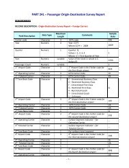
of government transportation expenditures. Stategovernments collected about half of these revenues,the federal government about one-third,and local governments about one-fifth. By mode,highways generated about 70 percent of theserevenues, followed by air (15 percent), transit (10percent), and water transportation (4 percent).From 1977 to 1994, federal transportationrelatedbudget receipts, including revenue fromtrust funds (taxes and user fees dedicated to aspecific mode), rose from $16 billion to $19.7billion (in constant 1987 dollars). The twolargest sources are the Highway Trust Fund(HTF)—which has highway and transitaccounts—and the Airport and Airway TrustFund. Of these, the aviation trust fund revenuesincreased the most, while HTF transit accountrevenues grew more slowly and HTF highwayaccount revenues declined slightly. Together, thetrust fund balances (unspent money in theseaccounts at the end of the year) grew substantiallyfrom the mid-1980s to the early 1990s, buthave declined from the 1992 high point.In 1993, governments at all levels invested$52.5 billion in transportation infrastructureand equipment. Most of the investment was forhighways, followed by airports and transit.In recent years, a good deal of research hasbeen devoted to assessing the economic returnsfrom government investment in public infrastructure,including transportation infrastructure.2 A recent study prepared for FHWA byNadiri and Mamuneas offers strong evidence onthe many ways highway capital in the UnitedStates contributes to the productivity of 35 differentindustries and the overall economy. In particular,it suggests that in the first two decades ormore while the Interstate highway network wasexpanding the overall economic benefits werehigh—with the return on the investment of a dolxvi Transportation Statistics Annual Report 1997place within firms that are not primarily engagedin providing transportation services to the public(e.g., a manufacturing plant or a grocery storechain). Although in-house providers of transportationare very important, current information isinsufficient to estimate their contribution. BTS andthe Bureau of Economic Analysis of the U.S.Department of Commerce are conducting a jointproject, called the Transportation SatelliteAccount, to develop a more complete picture of thetransportation industry, including in-house transportationservices.Household and government expenditures alsoindicate transportation’s economic importance.Transportation’s share of household expenditureswas 19 percent in 1994. The largest shareof household expenditures was housing, followedby transportation, and then food.Household expenditures on transportation varysignificantly by income. In 1994, transportation’sshare of household expenditures rangedfrom 14.1 percent for the $5,000 to $10,000income category to 22.1 percent for those in the$40,000 to $50,000 income category.Total government expenditures for transportationwere $116 billion in 1993. State andlocal governments contribute the lion’s share ofpublic expenditures for transportation. From1983 to 1993, their share (excluding federalgrants) rose by 38 percent in real terms; federalspending on transportation during that periodonly increased by 15 percent, resulting in adecline in the federal share of government transportationexpenditures from 37 to 32 percent. In1993, about 60 percent of government expenditureswere for highways, followed by transit (19percent), air (15 percent), and water transportation(5 percent). Rail and pipelines togetheraccounted for less than 1 percent.In 1993, government revenues from gasolinetaxes and other transportation-related taxes andfees totaled $85 billion, and covered 73 percent2See Transportation Statistics Annual Report 1995 for anindepth discussion of public investment in transportation.

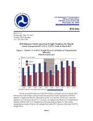
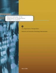
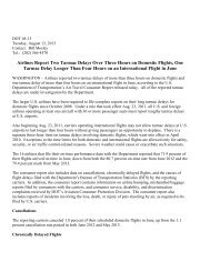
Statement of the Director xviilar in highway infrastructure greater than thereturn on a dollar of private capital investment.As the Interstate Highway System neared completionin the 1980s, the rate of return on highwaysfell gradually to just under the return onprivate capital investment in the economy.Transportation is also a major source ofemployment. Employment in the for-hire transportationindustry (3.9 million people) could beadded to employment in transportation occupationswithin nontransportation industries to estimatethe number of people employed intransportation functions. The resulting figure of5.8 million employees, however, is a low-end estimate.For example, it excludes people who arenot in transportation occupations who nonethelesswork full time in transportation activities innontransportation industries. Nor does it includemost employees in such transportation-relatedfunctions as transportation equipment manufactureor in government. If all of these jobs areAnnual Rate of Return by Type of InvestmentPercent403530252015105035133514Total highway capitalPrivate capital1950–59 1960–69 1970–79 1980–89SOURCE: M.I. Nadiri and T.P. Mamuenas. 1996. Contribution of HighwayCapital to Industry and National Productivity Growth, prepared for theU.S. Department of Transportation, Federal Highway Administration,Office of Policy Development. September.16121011counted, employment in transportation and relatedindustries has fluctuated around 9.9 millionsince 1990.Transportation and SafetyIn the United States, transportation has accountedfor roughly half of accidental deaths for manyyears. Transportation fatality trends show thatcommercial airlines, buses, and railroads are thesafer passenger modes. Travel by private vehicle—whethera car or light truck, a recreationalboat, or personal use aircraft—is less safe. In1995, more people died in recreational boatingand general aviation crashes than were killed aspassengers on trains, buses, or planes in commercialaviation combined.Crashes involving motor vehicles accountedfor 41,798 fatalities in 1995—some 94 percentof the transportation deaths that year. An estimated3.5 million people were injured in crashesinvolving motor vehicles. Motor vehicle crashesare the leading cause of death for Americansuntil their mid-thirties, except for the veryyoungest children. The National HighwayTraffic Safety Administration (NHTSA) estimatesthat the costs to the economy over the lifetimesof those injured or killed in motor vehiclecrashes in 1994 will be $150.5 billion. Thisamount does not attempt to estimate the dollarvalue of the loss of quality of life.Despite the huge toll—115 people died andover 9,500 people were injured in highwaycrashes each day in 1995—remarkable improvementin highway safety has occurred in the lastthree decades. The greatest number of deathsoccurred in 1972, when 54,589 people werekilled in crashes involving motor vehicles. Hadthe 1969 death rate of 5.0 fatalities for every 100million vehicle-miles traveled (vmt) persisted,more than 120,000 people would have diedfrom motor vehicle crashes in 1995, comparedwith the actual figure of 41,798 fatalities (about

xviii Transportation Statistics Annual Report 1997Occupant FatalitiesFatalities per 100 million vehicle-miles6050403020321MotorcyclesPassenger carsLarge trucks01975 1980 1985 1990 1995SOURCE: See figure 3-1 in chapter 3.1.7 fatalities for each 100 million vmt). Theimprovement was evident in most categories ofvehicles, even though the rates vary greatly.Many factors, including installation and use ofsafety innovations, better highway design, safetystandards and regulations, education efforts, andimproved emergency and medical care, havehelped reduce the fatality rate.Since 1992, however, the fatality rate has beenstable, portending an increase in the number offatalities if vmt continues to increase. Many fatalitiescould be avoided if more drivers, occupants,and pedestrians followed well-known safety precautions.In 1995, 17,274 people died in alcoholrelatedcrashes— 41 percent of all people killed inhighway crashes. Excessive speed or driving toofast for conditions was a contributing factor in 31percent of fatal crashes. (Often, fatal crashesinvolve speeding and drinking). While safety beltuse has increased over the years, nearly one-thirdof passengers still do not buckle up. NHTSA estimatesthat there would be 9,835 fewer fatalities ifeveryone used safety restraints.Although they involve far fewer fatalities intotal than private vehicles, fatal crashes involvingcommercial vehicles—especially airplanes, trains,and buses—receive great scrutiny from safetyorganizations, the press, and the public, in partbecause a single crash can involve dozens or, insome cases, hundreds of deaths. Two plane crashesin 1996—the crash of ValuJet Flight 592 intothe Florida Everglades and the crash of TWAFlight 800 off Long Island Sound—have been thesubject of extensive investigation by safetyauthorities, and received prime time coveragefrom the media for many weeks, putting a spotlighton aviation safety. With air travel growing inpopularity, aviation safety will continue to be aprominent concern of the traveling public.Travel by commercial airline is much safertoday than it was three decades ago, whenabout 10 people died for every 100,000 planedepartures on U.S. air carriers. Since 1992, therate has fluctuated between 1 and 2 fatalitiesper 100,000 departures. (Because crashes areinfrequent, this rate is expressed as a 5-yearmoving average to even out large year-to-yearvariations.) The most robust improvement (asshown in the moving average) occurred in the1960s and the 1970s; since then, the improvementhas slowed.Safety data are collected separately for eachindividual mode. There is, however, increasinginterest in examining safety trends on a crossmodalor systemwide basis. This year’s safetychapter addresses four cross-modal issues: thesafety of children in the transportation system;safety of workers in transportation occupationsor occupations that require frequent use of transportation;transportation of hazardous materials;and efforts to develop common measures ofsafety across the modes.

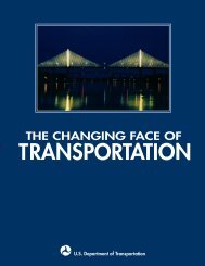
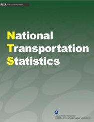
Statement of the Director xixU.S. Petroleum Use and Imports403530252015105Quadrillion BtuTotal petroleum useTransportation petroleum useNet imports of petroleum01970 1975 1980 1985 1990 1995SOURCE: See figure 4-7 in chapter 4.Energy and the EnvironmentFor nearly half a century, transportation hasaccounted for about one-quarter of total U.S.energy use. Between 1994 and 1995, transportationenergy use grew by 1.7 percent—a rate ofgrowth similar to that which has occurred since1985. In contrast, transportation energy usegrew by only 0.6 percent annually between 1973and 1985, when oil supply shocks and higherprices dampened demand and inspired majorimprovements in energy efficiency.Petroleum-based fuels are used to satisfyalmost all (95 to 97 percent) of U.S. transportationenergy demand. Transportation accountsfor about two-thirds of the nation’s demand foroil. Despite recent gains in the number of alternativefuel vehicles and the greatly increased useof alcohols and ethers in gasoline to satisfy mandatedcleaner fuel requirements, nonpetroleumfuels still supply a small share.Approximately half of the petroleum consumedin the United States must be imported.Petroleum dependence is of concern because theworld’s oil reserves are increasingly concentratedin relatively few countries. The Organization ofPetroleum Exporting Countries (OPEC) holdstwo-thirds to three-quarters of the world’sproven reserves and more than half of theworld’s estimated resources. In the past threeyears, however, increased production in theNorth Sea and other nontraditional producingareas stabilized the market influence of OPECand kept prices low. As these relatively smallreserves are depleted, OPEC market share andinfluence likely will grow. World dependence onOPEC oil is expected to rise from today’s 40 percentto 52 percent in 2010 and 56 percent by2015, levels similar to those of the early 1970s.Concentration of production can lead to pricevolatility and upward pressure on prices, even ifno supply disruption occurs. The potential forvolatility in petroleum markets was illustrated inthe spring of 1996, when a confluence of factors,including higher crude prices, low inventories,and a surge in demand, caused a greater thannormal seasonal increase in gasoline prices.Average gasoline prices rose almost 22¢ per gallon,in contrast to a typical seasonal increase of5¢ per gallon. This jump renewed public concernabout the operation of petroleum markets andthe nation’s dependence on petroleum.It appears that the transportation sector hasreached the end of a 20-year period of steadilyimproving energy efficiency. Although somemodes, such as air passenger travel and railfreight, continue to show efficiency gains, thisis offset by a decline in the energy efficiency ofhighway travel. (Accounting for the vastmajority of all passenger-miles, the highwaymode dominates U.S. passenger travel andenergy use trends.) Bus and rail transit modesalso showed higher energy intensity.BTS’s analysis shows that cumulative energysavings from changes in transportation energyefficiency declined between 1993 and 1994—the

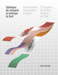
the first drop since 1992 in volatile organic compoundsemissions. Reductions in onroad vehicleemissions accounted for the lion’s share of therecent reductions; emissions from aircraft and airportservices vehicles also decreased. (Lead emissionsfrom transportation have been all buteliminated for several years.)Transportation-related greenhouse gas emissionscontinue to follow trends prevalent over thepast several years. Carbon dioxide emissions bytransportation continue to rise due to increasedenergy use. Since 1990, transportation has accountedfor nearly 40 percent of the nationalincrease in carbon dioxide emissions from endusesectors, with potentially serious implicationsfor global climate change.Strides have been made in understanding,quantifying, and reducing some other environmentalimpacts of transportation. For example,federal noise standards have reduced exposure tounacceptable levels of aircraft noise, and the governmentcontinues to monitor underground storagetank releases and cleanup efforts. Otherimpacts, such as land use and habitat fragmentaxx Transportation Statistics Annual Report 1997first time since 1985. Average miles per gallon oflight-duty vehicles, now 24.6, has not changedsignificantly since 1979. Technological improvementswere largely offset by increasing vehicleweight and power and decreasing vehicle occupancyrates.The energy efficiency of air travel has continuedan unbroken 22-year trend of improvement.The biggest factor was an increase in load, butimproved aircraft efficiency accounted for aboutone-third of the improvement. Like air travel,rail freight energy efficiency has made steadygains for two decades. Many factors have contributedto efficiency gains, including improvedoperating practices that have greatly reducedengine idling and improved train pacing, lighterweight cars, and new locomotive technologies. Environmental ImpactsBecause of its enormous size and activity, the U.S.transportation system inevitably has undesirableenvironmental impacts. 3 Air pollution is the moststudied environmental impact and has been thesubject of extensive remedial action, air qualitymonitoring, and data collection. Transportationaccounts for two-thirds of carbon monoxide (CO),42 percent of nitrogen oxides, and nearly one-thirdof the hydrocarbons produced.Despite a doubling in highway vehicle-miles,most highway vehicle emissions are far lowertoday than in 1970, reflecting emissions controlsadopted under federal clean air requirements.The record of success has not been uniform, however.There were increases in some transportationemissions in 1992, 1993, and 1994 comparedwith previous years. According to the latest U.S.Environmental Protection Agency estimates,progress was made in 1995, with, among otherthings, a major reduction in CO emissions and3See Part II of Transportation Statistics Annual Report1996 for a comprehensive discussion of transportationrelatedenvironmental issues.Selected Air Emissions from Transportation1.41.21.00.80.6Index (1970=1)Nitrogen oxidesCarbon monoxideVolatile organic compounds0.41970 1975 1980 1985 1990 1995NOTE: Transportation emissions include all onroad mobile sources andthe following nonroad mobile sources: recreational vehicles, recreationalmarine vessels, airport service equipment, aircraft, marine vessels, andrailroads.SOURCE: See figure 4-10 in chapter 4.

Statement of the Director xxition, are less well understood, and thus more difficultto assess or quantify.The State of Transportation StatisticsWhen Congress, through the Intermodal SurfaceTransportation Efficiency Act of 1991 (ISTEA),created the Bureau of Transportation Statistics,the purpose was to enhance the transportationknowledge base and to inform the public abouttransportation and its consequences. To that end,Congress called on BTS to document the methodsused to obtain information and to ensure thequality of statistics used in this annual report,and to include in the report “recommendationsfor improving transportation statistical information.”Because ISTEA’s authorization for federalspending ends with fiscal year 1997, Congress isnow evaluating alternative authorization optionsfor these programs in the future. Thus, this 1997annual report comes at an opportune time toreview the path followed by BTS and other information-producingagencies, and examinewhether that path is appropriate for the start ofthe next century. Chapter 5, summarized below,discusses progress and challenges in meetingISTEA information needs, suggests ways inwhich the world of information may change, andindicates some future directions that decisionmakersmight consider for transportation statisticsprograms.BTS has taken many actions to fill data andknowledge gaps and needs identified in theISTEA. Among other things, the Bureau has: published four transportation statistics annualreports, as well as annual compendiums ofnational transportation statistics; completed national surveys of commodity andpassenger flows by all modes and intermodalcombinations; initiated efforts with Canada and Mexico toproduce a continental view of North Americantransportation; established a standard classification of transportablegoods; become a leader in developing geographicinformation systems databases; and actively disseminated information, usingprinted and newer electronic means.The ISTEA provided a good start towardmeeting critical information needs, but severaltopics remain for which more or better informationare needed. These include: 1) domestic transportationof international trade; 2) timeliness andreliability of transit, highway travel, and freightmodes; 3) costs of transportation services; 4)more reliable information on the number ofmotor vehicles by vehicle class, and distances theyare driven; 5) fuller information on the location,connectivity, capacity, and condition of railroadlines; and 6) interactions among transportation,economic development, and land use.Needs for information and technologies formeeting these needs continue to evolve rapidly.Statistics on cost and service quality, involvingtimeliness and reliability, and not just forecasts oftraffic volume and capacity are needed. Involvementby metropolitan planning organizations,private sector interests, and citizen organizations,as well as federal and state agencies, hasincreased the number and range of customersdemanding data and the tools to use the data.The Government Performance and ResultsAct of 1993 (GPRA) is also affecting the need forstatistical information. GPRA requires all federalagencies to begin measuring their outcomes,and not just their inputs and outputs. GPRA is tobe the basis of budget decisions by the Office ofManagement and Budget and will be monitoredby Congress. GPRA’s focus is prompting manyagencies to become aware of the conditionsbeing measured by BTS and other statisticalagencies. Most state departments of transportationand some local agencies also are undertakingperformance measurement efforts.

xxii Transportation Statistics Annual Report 1997Decentralization of decisionmaking, eitherfrom the public sector to the private sectorthrough deregulation or from the federal governmentto state and local governments, is potentiallythe biggest change in transportation policyto be informed by statistics. Although decentralizationcould reduce the federal role in manyareas, the need for publicly available transportationstatistics may grow. The free flow of informationis often a prerequisite to properlyfunctioning private markets, and state and localofficials need to relate conditions within theirjurisdictions to national and international trends.In response to customer demands, BTS proposesto build on its initial products and serviceswith three major initiatives. These initiatives arepart of the Administration’s proposed NationalEconomic Crossroads Transportation EfficiencyAct (NEXTEA). They include: expanded programsof data collection, and the development ofa knowledge base involving international transportationin a globalized economy; expandedservices and grants to state, local, and privatedecisionmakers to enhance data collection andsharing throughout the transportation community;and a program of research, technical assistance,and data-quality enhancement to improveperformance measurement. These proposals arediscussed in detail in chapter 5.PART II: MOBILITY AND ACCESSPart II explores mobility’s importance in theAmerican society and economy, and the transportationsystem’s facilitating role in providingaccess to opportunities. Mobility, as used here,refers to the potential for movement. It expandsthe geographic choices available to people andbusinesses. Today’s level of personal mobility (asreflected in miles traveled per capita) is unparalleledin U.S. history. Mobility can enhance theability of people to participate in economic andsocial life, expanding personal freedom andchoice. Mobility helps businesses serve new markets,provides more choices for locating facilities,broadens their range of suppliers, and increasesthe available pool of workers.Accessibility refers to the potential for spatialinteraction with various desired social and economicopportunities. Accessibility varies for individualsand across regions. Part II describes suchvariations in accessibility in the context of barriersto movement, such as age, location, disbility,and the lack of availability of vehicles or transportationservices.Part II also examines advances in informationtechnologies (IT), and their ramifications fortransportation. Transportation firms and theircustomers are adopting a number of generic informationtechnologies made possible by advances intelecommunications and computers. IT is transformingthe way these firms do business in a mannerreminiscent of the change wrought ontransportation and the broader economy in the19th century by the telegraph and the railroad.This IT transformation is discussed in terms ofchanges in the nature of transportation demandand the supply of new transportation services, andin the emerging pattern of activities, managementstructures, and competition both among transportationproducers and among their customers.Part II discusses six topics: concepts of mobility and access, personal mobility in the United States, access to opportunity, freight, the international context, and mobility and access in the information age.Concepts of Mobility and AccessibilityMobility is measured by the movement of peopleand materials on the transportation system. Accessibilityis measured by the ease of reaching thelocation of a desired activity from another place.

Statement of the Director xxiiiMeasurements of mobility and accessibilitycan be helpful in evaluating the performance oftransportation. A number of methodological difficulties,however, limit their use. Of the twoconcepts, accessibility is the more difficult tomeasure, but measuring mobility is not especiallyeasy. Because of data gaps, there is often littlealternative to using indirect measures.Analysts have employed the concept of revealedmobility (defined as the number of milestraveled or trips taken over some unit of timesuch as a day, week, or a year) as an imperfectproxy for mobility. The assumption in usingrevealed mobility is that, all else being equal,people taking many trips or traveling manymiles have a higher level of mobility. Thisassumption is not always borne out, however.For example, revealed mobility data would registera mobility decline if a commuter moves toa residence closer to work. Yet, having to travelfewer miles to work or spend less time commutingis not in any meaningful sense a decline inmobility. Despite such problems, revealedmobility can be a useful analytical tool, andhelps explain a great deal about travel behaviorand shipping activities.Accessibility measures can be useful in evaluatingtransportation access to locations wheredesired activities (e.g., employment, shopping,health care, and recreation) take place. They alsocan help identify access problems of people withlimited transportation options. Several accessibilitymeasures have been developed, includingrelative accessibility (measuring one location relativeto another) and integral accessibility (integratinginformation about locations of severalactivities). Accessibility also encompasses a timeelement. While there may be several shops locateda short distance from a person’s home, theywill not be accessible if they close for businessbefore the person can get there from work, or donot open until after the commuter leaves home.The concept of accessibility applies to firms aswell. Manufacturing firms benefit if their suppliersand markets for their products are easilyaccessible, and if a large pool of workers is withincommuting range. Retail stores and other servicefirms have an advantage if their location ishighly accessible to a large number of potentialcustomers. Firms that produce or use bulkymaterials need access to low cost transportation(e.g., railroads or waterways). If transportationtime is more critical than cost, proximity to anairport may be needed for accessibility.On a broad scale, accessibility can criticallyaffect the economic prospects of entire regions.In the 19th century, Chicago’s location as themain hub of a network of railroads gave itunmatched accessibility among midwesterncities. More recently, accessibility to Pacific Rimmarkets has been an impetus to growth in westcoast port cities.Measurement of accessibility requires informationnot only about travel but about the locationof destinations. This task has become morecomplicated, reflecting multiple locations offacilities and activities in most urban regions.While once travel time to the central businessdistrict from a residential area may have sufficedas an indication of relative accessibility, today,relative accessibility measures might includeaverage travel time or cost to the nearest shoppingmall, hospital, or park.Because of the variety of opportunities availablein most urban areas, integral accessibilitymeasures provide a better picture of the ability toreach many desired destinations. These measuresare harder to construct, however, as they mustcombine information about many routes anddestinations.Developing appropriate accessibility indicatorsat different geographic scales is an importantchallenge. It is possible to developaccessibility measures for a zone or region—by

xxiv Transportation Statistics Annual Report 1997taking an average of a number of points within azone. It is also possible to map patterns on abroader geographic scale by calculating accessibilityat different points.Average Daily Miles of TravelPerson in household withincome over $40,000Passenger-milesper day38Personal Mobility in the United StatesAmericans travel more than ever, and continueto increase their use of the transportation system.Growth in passenger travel reflects many differentfactors, including population and labor forcegrowth, a decline in household size, incomegrowth, and dispersion of development andemployment centers within metropolitan areas.Four Nationwide Personal TransportationSurveys (NPTS) conducted between 1969 and1990 provide detailed information about travelbehavior of specific groups. (Results from the 1995NPTS and BTS’s American Travel Survey (ATS),also conducted in 1995, are not yet available. TheATS focuses on travel of more than 75 miles fromhome, while NPTS emphasizes daily trips.)On average, most groups—men and women,young and old, rich and poor, city and rural residents—traveledmore each day in 1990 than in1969. Pronounced differences abound, reflectingboth travel needs and the ability to travel. Forexample, suburban residents travel about 32 milesper day, slightly more than rural residents, and 30percent more than central-city residents (just over24 miles per day). People with higher incomestravel farther than those with lower incomes.People in the 40- to 49-year-old age group travelmore than their younger or older age cohorts.Men travel further than women, on average,although women make slightly more daily trips.Whites travel further than blacks or Hispanics.The availability of a passenger car or vehiclemakes a critical difference. People relied on carsand other privately owned vehicles for 87 percentof their daily trips in 1990. Transit accountedfor 2 percent of trips. All other modes(including airplanes, Amtrak, taxi, walking,DriverRural residentU.S. averageCentral-city residentPerson in household withincome under $10,000NondriverSOURCE: See figure 7-1 in chapter 7.bicycling, and school buses) accounted for theremaining 11 percent.The number of households without a car orother passenger vehicle declined from 21 percentin 1960 to 11.5 percent in 1990; still, 10.6 millionhouseholds did not have a car in 1990. Theability to drive a passenger car has had an enormousimpact on mobility. In 1990, people withdrivers licenses took nearly twice as many dailytrips, traveled three times as far, and took longertrips than people without licenses.More than one-third of the travel by the averageperson involved social and recreational purposes;another third involved family and personalbusiness (e.g., shopping and doctor’s appointments).About one-quarter of the travel miles and22 percent of trips are to and from the workplace.Work trips, however, are more importantthan the figure suggests. Many people shop andconduct other personal business during theircommute to and from work. If such trip chaining343029241611

Statement of the Director xxvis added to simple work trips, then people structure30 percent of their daily trips around theirwork schedule. While trip chaining during thework commute increases peak hour travel, it alsomay allow people to choose to make fewer tripsand to travel fewer miles overall.Access to OpportunitiesOn a nationwide basis, access has increased sincethe end of World War II reflecting the effects offurther urbanization, the development of transportationfacilities (particularly the completion ofthe Interstate Highway System and the expansionof the air transportation industry), and economicdevelopment. Despite these improvements, someareas of the country, experienced a decline in sometypes of transportation services. Fewer places areserved today by passenger rail and intercity buses,in part because carriers have given up unprofitableor sparsely used services. Rural areas have beenespecially affected by such changes.In urban areas, access has generally increased,although much of that access depends on theautomobile. Transit service, too, is accessible tomany urban residents. In 1990, half of thehouseholds in urban areas were located withinone-quarter mile of a transit route, close enoughfor most people to walk. Transit, however, hashad a hard time keeping up with the changingspatial distribution of opportunities, particularlyjob sites. Many poor people in central cities havevery limited access to employment opportunitiesin the distant suburbs, the location of much newemployment growth, including entry-level jobs.Insufficient transportation options are part of theexplanation, as many urban poor people do nothave cars and public transit stops are often lackingnear suburban job locations. This will presenta transportation challenge for many welfarerecipients in central-city areas who will soonneed employment due to changes in federal andstate welfare programs.Access to transportation is increasing for personswith disabilities, although challenges remain.Under the Americans with Disabilities Actof 1990, fixed-route service is to be madeincreasingly available to the disabled, with paratransitthe recourse when fixed-route transitdoes not meet a customer’s needs or is inappropriateto the situation. Paratransit accounted for37 million trips in 1995. The evolving relationshipbetween fixed-route transit and paratransithas several implications. For example, fixedrouteservice needs to be designed so as to beaccessible to persons with disabilities (e.g., liftson buses, and elevators and raised platforms atkey train stations), and drivers need training onproper use of equipment. Fixed-route and paratransitservices will now need to be coordinatedand developed together, taking advantage ofnewly available information technologies. Withgreater accessibility, transit demand by the disabledhas increased and will likely increase inthe near future.Mobility from the Freight PerspectiveBecause of the widespread availability of transportationand advances in information technologies,U.S. businesses are able to transport rawmaterials, finished goods, and people quickly,cheaply, and reliably, often across great distances.On a typical day in 1993, about 33 milliontons of commodities, valued at about $17billion, moved an average distance of nearly 300miles on the U.S. transportation network. Theseestimates are based on data from the CommodityFlow Survey (CFS), 4 the most extensivesurvey of domestic freight movements undertakensince 1977, and supplemental data on waterborneand pipeline shipments. Even this largefigure underestimates total freight movements,4BTS calculated the daily total from final CFS data plusadditional data on waterborne and pipeline shipments notfully covered by the CFS.

xxvi Transportation Statistics Annual Report 1997as it does not include most imports and someother flows.In 1993, domestic establishments in the sectorscovered by the CFS shipped materials andfinished goods weighing 12.2 billion tons, generating3.6 trillion ton-miles within the UnitedStates. The goods shipped were valued at morethan $6.1 trillion. The food and kindred productssector accounted for the highest dollaramount of shipments identified in 1993, followedby transportation equipment. The majorcommodities by weight were petroleum and coalproducts, nonmetallic minerals, and coal. Foodand kindred products ranked fourth by weight.The major commodities vary greatly whenranked by the value per ton of shipment. Onaverage in 1993, high-value commodities (e.g.,worth over $5,000 per ton) accounted for 41 percentof the total shipments but only 2 percent ofthe tons and 5 percent of the ton-miles. Lowvaluecommodity categories (e.g., those that averagedless than $1,000 per ton) accounted for lessthan half of the value, yet accounted for most ofthe tons and ton-miles, 96 percent and 91 percent,respectively.A large portion of the shipments by valueoriginate in states with a major manufacturingbase, such as California, New York, Michigan,Texas and Illinois. These states were also the destinationsfor a large portion of shipments.Manufacturing, however, is an important activityin most states. Partly because firms are able tocheaply and reliably transport materials, parts,and merchandise from one part of the country toanother, industrial production is dispersedthroughout the United States.Raw materials and processed goods areshipped to all parts of the nation. For example,enormous amounts of farm products travel fromnorth to south on the Mississippi River forexport from Gulf coast ports. During the pastthree decades, the pattern of coal movement hassignificantly changed. Before the 1970s, about95 percent of domestically produced coal wasmined east of the Mississippi River. By 1995,more than 47 percent of U.S. coal was producedin the western states. This growth is partly due toincreased demand for low-sulfur coal mined inMontana and Wyoming.Trucking was the most dominant mode forfreight transportation in 1993, moving about 72percent by value and 53 percent by weight ofshipments, and producing 24 percent of tonmiles.Rail freight produced slightly more tonmiles,26 percent of the total, and accounted for13 percent of the weight of shipments but just 4percent of the value. Waterborne transportationaccounted for over 17 percent of tons and 24percent of ton-miles. The classic intermodalcombination of truck and rail moved over 40million tons of commodities worth over $83 billion.Parcel, postal, and courier services wereused to move over 9 percent of the value of shipmentsvalued at over $560 billion.The distribution of freight carried by the differentmodes in part reflects changes occurring inthe economy. Today, high value-adding businessesoften require quick, reliable, and high-qualitytransportation to assure faster product deliveries,on time, with little product loss or damage. Forexample, parcel, postal, and courier serviceswere used to transport nearly one-quarter of theshipments of electrical equipment, machinery,and supplies in 1993. Business uses of moreexpensive truck and air transport fit a pattern ofdynamic, globalized economic activity movingtoward lower overall costs of production andproduct distribution.The transportation system also is used to provideother essential services to the economy.About 16 million households moved in 1994.Over 200 million tons of solid waste were collectedby municipalities for recycling, incineration,or disposal in 1994. Most was transported

Statement of the Director xxviiSum of Imports and Exports of Goods1,5001,2501,0007505002500Chained 1992 dollars (billions)276SOURCE: See figure 9-10 in chapter 9.1,3111970 1995a few miles, but some was shipped as much as2,000 miles for disposal.The nation’s transportation network facilitatesan interconnected economy both nationallyand internationally. Imports and exports ofgoods and services have grown rapidly. Since1970, international waterborne freight movingto and from U.S. ports has nearly doubled byweight. As businesses transport enormousamounts of goods within and among states, thenation’s economy becomes more connected.Nationally, about 62 percent of the value and 35percent of the weight of shipments by all modeswere interstate. These estimates from the CFSshow the national dimensions of freight movementwithin the United States.International Trends in PassengerMobility and Freight ActivityAmericans traveled more than 24,000 passengerkilometers(pkm) per capita in 1991, surpassingEuropeans at 12,000 pkm and Japanese at 11,000pkm. The United States also leads all countries infreight intensity with almost 20,000 metric tonkilometersper capita in 1994 compared with10,000 in Canada and about 4,500 in Japan.As national economies and real personalincome increase in most parts of the world, passengercars and trucks are replacing rail and busservice and nonmotorized transportation forboth passenger travel and freight activity. Airtransportation is generally the fastest growingmode (but it holds a small overall modal share).Although changes in passenger travel and freightmovement are evident in all regions of the developingworld except some parts of Africa, thepace and extent of change varies greatly.In the United States, cars and light trucksdominate passenger travel, accounting for 86percent of passenger-miles traveled in 1994.Passenger cars account for about 80 percent ofpkm in Western Europe. In Japan, by contrast,only about half of travel takes place in passengercars, in part reflecting the importance of intercityand urban rail services in the high-populationdensitycorridor between Tokyo and Osaka.The number of passenger cars in use has beengrowing faster than the population in the developedcountries. Automobile growth, however, isthe highest in some developing countries, especiallythe rapidly growing economies in Asia.,Passenger-Kilometers Traveled by ModePercent100Cars Rail908070BuseșAir86806052504030, 201000.5 110USA (1994)SOURCE: See figure 10-1 in chapter 10.695EuropeanUnion (1993)3395Japan (1994)

Statement of the Director xxixexpress for the movement of documents, oravoid intercity trips through conference calls.Such options are affecting commercial operationsand daily life.Transportation-related enterprises, like mostbusinesses, are being changed by IT. The “bottomline” in transportation applications of IT isdetermined by the balance between cost and service.IT can affect both strongly. The acquisitionand processing of operational, financial, andrelated data directly support higher systemcapacity, greater labor and capital productivity,improved efficiency, more effective resource allocation,and better integration of the manyprocesses and activities that cumulatively producetransportation services.Detailed understanding of system operationsenables the design and implementation of innovativeoperational concepts and practices. Theovernight package delivery service, for example,could hardly exist on its present scale without amyriad of computers, digital tags on each item,and extensive communications links. Similarly,computerized reservation systems are critical tothe operation of the commercial aviation system,which fills well over 1 million airline seats eachday for several thousand origin-destination pairsat market-driven prices.Information technologies are beginning totransform the interface between the serviceprovider and the customer or user. The implementationof intelligent transportation systems(ITS) includes as a basic component the provisionof real-time status information for localhighways and transit systems, potentially withguidance as to optimal choices for particulartrips. An individual sending a package for nextdaydelivery can use the Internet to track itsprogress. With a highly controlled and visibletransportation system, manufacturers can safelyintegrate their suppliers into just-in-time productionsystems and tailor their outputs to shorttermcustomer needs.Information technologies also can alter theneed to travel, or the type of transportationconsumed. Personal purchases may be made bytraveling to a store, or by ordering (using thetelephone or the Internet) and relying on adelivery service. Aided by modem-equippedcomputers, fax machines, and online services,some people find it feasible—and often preferable—towork from home, either as a telecommutingemployee or as an independent businessor contractor.Most transportation uses of IT depend on theintegration of many specific technologies andcapabilities. Improvements in one technical areamay make new applications or services available.The full impact of the IT evolution for transportationis likely to emerge slowly in the comingdecades, and often will not be separable from theeffects of other societal changes. BTS has published a companion volume tothis report, National Transportation Statistics1997 (NTS), which covers the 1960 through1995 time period. NTS provides modal profilesand statistics on the state of transportation, theeconomic importance of transportation, safetytrends, and energy and environmental aspects oftransportation. Most of the NTS tables, as wellas many other BTS products, are available on theBTS Internet homepage. Information about contactingBTS is on the back cover of this report.T.R. LakshmananDirector

Part I▼The State of the Transportation System▼

chapter oneTheTransportationSystemThe United States has the world’s largest transportation system, serving the265 million people and 6 million business establishments that occupy thefourth largest nation by land area. The interlocking elements of the transportationsystem include not only the physical links among places—highways, transitsystems, railroads, airports, waterways and ports, and pipelines—but the firmsthat provide transportation services, the many industries that produce and maintainvehicles, and agencies with transportation responsibilities at all government levels.Americans are highly mobile and American businesses ship more freight per capitathan any other country. Passenger-miles per person averaged 16,500 miles in 1995(not including miles traveled in heavy trucks), while 12,600 ton-miles of freight weregenerated per capita. The transportation facilities that made this possible included,among other things, 3.9 million miles of public roads, 170,000 miles of railroadtrack operated by freight carriers, 44,000 transit buses, 40,000 U.S.-flag vessels, and200,000 miles of oil pipelines (see table 1-1). These transportation facilities supported4.3 trillion miles of passenger travel and 3.6 trillion ton-miles of goods movement.(USDOT BTS 1996, 15, 20)This chapter provides an overview of the extent, use, condition, and physicalperformance of the transportation system, updating the discussion in earlier editionsof the Transportation Statistics Annual Report. For 1997, one mode, urban3

4 Transportation Statistics Annual Report 1997Table 1-1.Major Elements of the Transportation System: 1995Mode Major defining elements ComponentsHighways 1AirRail 5Public roads and streets; automobiles,vans, trucks, motorcycles,taxis, and buses (except local transitbuses) operated by transportationcompanies, other businesses, governments,and households; garages,truck terminals, and other facilitiesfor motor vehiclesAirways and airports; airplanes,helicopters, and other flying craft forcarrying passengers and cargoFreight railroads and AmtrakPublic roads45,744 miles of Interstate highway111,237 miles of other National Highway System roads3,755,245 miles of other roadsVehicles and use136 million cars, driven 1.5 trillion miles58 million light trucks, driven 0.7 trillion miles6.9 million freight trucks, driven 0.2 trillion miles686,000 buses, driven 6.4 billion milesPublic use airports5,415 airportsAirports serving large certificated carriers 229 large hubs (67 airports), 393 million enplanedpassengers33 medium hubs (59 airports), 86 million enplanedpassengers58 small hubs (73 airports), 34 million enplanedpassengers561 nonhubs (593 airports), 14 million enplanedpassengersAircraft5,567 certificated air carrier aircraft, 4.6 billion miles flown 3Passenger and freight companies86 carriers, 506 million domestic revenue passengerenplanements, 12.5 billion domestic ton-miles of freight 3General aviation181,000 aircraft, 2.9 billion miles flown 4Railroads 6125,072 miles of major (Class I) 718,815 miles of regional26,546 miles of local24,500 miles of AmtrakEquipment1.2 million freight cars18,812 freight locomotivesFreight railroad firmsClass I: 10 companies, 185,782 employees, 1.3 trillionton-miles of freight carriedRegional: 30 companies, 10,647 employeesLocal: 500 companies, 13,269 employeesPassenger (Amtrak)23,646 employees, 1,722 passenger cars, 8 313 locomotives,8 20.7 million passengers carried 9

Chapter 1 The Transportation System 5Table 1-1.Major Elements of the Transportation System: 1995 (continued)Mode Major defining elements ComponentsTransit 10WaterPipeline 14Commuter trains, heavy-rail (rapidrail)and light-rail (streetcar) transitsystems, local transit buses, vansand other demand response vehicles,and ferry boatsNavigable rivers, canals, the GreatLakes, the St. Lawrence Seaway,Intracoastal Waterway, and oceanshipping channels; ports; commercialships and barges, fishing vessels,and recreational boatsCrude oil, petroleum product, andnatural gas linesVehicles43,577 buses, 17.0 billion passenger-miles8,725 rapid rail and light rail, 11.4 billion passenger-miles4,413 commuter rail, 8.2 billion passenger-miles68 ferries, 243 million passenger-miles12,825 demand response, 397 million passenger-milesU.S.-flag domestic fleet 11Great Lakes: 698 vessels, 60 billion ton-milesInland: 31,910 vessels, 306 billion ton-milesOcean: 7,033 vessels, 440 billion ton-milesRecreational boats 12 : 11.7 millionPorts 13Great Lakes: 362 terminals, 507 berthsInland: 1,811 terminalsOcean: 1,578 terminals, 2,672 berthsOilCrude lines: 114,000 miles of pipe, 323 billion ton-milestransportedProduct lines: 86,500 miles of pipe, 269 billion ton-milestransported161 companies, 14,900 employeesGasTransmission: 276,000 miles of pipeDistribution: 919,000 miles of pipe19.7 trillion cubic feet, 150 companies, 187,200 employees1U.S. Department of Transportation, Federal Highway Administration. 1995. Highway Statistics. Washington, DC.2U.S. Department of Transportation, Bureau of Transportation Statistics, Office of Airline Information. 1996. Airport Activity Statistics of CertificatedAir Carriers, 12 Months Ending December 31, 1995. Washington DC.3Preliminary data.4U.S. Department of Transportation, Federal Aviation Administration. 1997. General Aviation and Air Taxi and Avionics Survey, Calendar Year 1995.Washington, DC.5Except where noted, figures are from Association of American Railroads. 1996. Railroad Facts. Washington, DC.6Miles of track operated.7Includes 891 miles of road operated by Class I railroads in Canada.8Amtrak. 1997. Twenty-Fifth Annual Report, 1996. Washington, DC.9Excludes commuter service.10U.S. Department of Transportation, Federal Transit Administration. 1997. National Transit Database, 1995. [cited as of 5 August 1997] Available atwww.fta.dot.gov/library/reference/sec15/1995/index.html.11Excludes fishing and excursion vessels, general ferries and dredges, derricks, and so forth used in construction work. Vessel data from U.S. ArmyCorps of Engineers. 1996. Transportation Lines of the United States. New Orleans, LA. Ton-miles data from U.S. Army Corps of Engineers. 1996.Waterborne Commerce of the United States,1995. New Orleans, LA.12U.S. Department of Transportation, United States Coast Guard. 1996. Boating Statistics. Washington, DC.13Ports data from U.S. Department of Transportation, Maritime Administration. 1996. A Report to Congress on the Status of the Public Ports of theUnited States, 1994–1995. Washington, DC. October.14Data are for 1994.SOURCE: Unless otherwise noted, U.S. Department of Transportation, Bureau of Transportation Statistics. 1996. National Transportation Statistics1997. Washington, DC. December.

6 Transportation Statistics Annual Report 1997transit, is profiled in detail. The chapter concludeswith a discussion of selected transportationevents that occurred in 1996. Otheraspects of the system’s performance, its economicrole and its unintended consequencesfor safety, energy import dependency, and theenvironment, are discussed in subsequentchapters of Part I of this report, which concludeswith an analysis of data and informationneeds in the rapidly changing world oftransportation.Passenger TransportationPassenger transportation, measured by passenger-milestraveled (pmt), continues to grow,and per capita travel growth appears to haveaccelerated during the last 25 years. Overall,pmt, excluding miles traveled by heavy trucks,grew from approximately 2.2 trillion in 1970to 4.3 trillion in 1995, a 2.7 percent averageannual increase. Again, excluding miles traveledby heavy trucks, per capita miles traveledin 1995 were 16,500, up from 11,000 in 1970,which was an annual rate of 1.6 percent overthe 25 year period—1.1 percent annually from1970 to 1980, 1.8 percent annually from 1980to 1990, and 2.3 percent annually from 1990to 1995. (USDOT BTS 1996)As discussed in more detail in chapter 7, manyfactors contribute to the increase in pmt. The residentpopulation increased by nearly 59 million,a rise of 29 percent between 1970 and 1995. Thenumber of people in the labor force, most ofwhom commute to work, grew twice as fast asthe population over the same period (from 83million to 132 million, a 59 percent increase).The number of working women and womenlooking for work increased from 32 million in1970 to 61 million in 1995. People also havemore money to spend on transportation, particularlyautomobiles and air travel. Disposablepersonal income per capita rose from $12,000 in1970 to $18,800 in 1995 (in chained 1992 dollars),a 56 percent increase. (USDOC 1996)The vast majority of pmt, 87 percent in 1995,took place in personal vehicles (including cars,light trucks, taxis, and motorcycles) (see figure 1-1). Despite enormous growth in pmt by personalvehicles, their percentage of total pmt declinedfrom 90 percent in 1970 because of the morerapid growth of air travel. Nearly 10 percent ofpmt was by air, 4 percent by transit, intercitybus, and school bus, and 0.3 percent by rail(both Amtrak and commuter rail). Passengermilestraveled in light trucks (including pickups,minivans, and sport utility vehicles) rose from 9percent of all pmt in 1970 to 21 percent in 1995.(USDOT BTS 1996)Despite the increase in motorized transportation,nonmotorized forms of transportationremain an important way to travel. In 1990,about 8 percent of all trips were made by nonmotorizedtransportation (7.2 percent on footand 0.7 percent by bicycle), a drop from 9.3 percentin 1983. (USDOT FHWA 1993, 4-58;USDOT FHWA 1986, 6-5) As pedestrian andbicycle trips are short, averaging 0.6 miles and 2miles, respectively, they accounted for less than 1percent of all person-miles in 1990. Because oftheir low cost, minimal impact on the naturalenvironment, and positive impact on publichealth, the U.S. Department of Transportationcarried out research to seek new ways to encouragewalking and bicycling to fulfill people’smobility needs. (See USDOT FHWA 1994)Trends in personal mobility are discussed inmuch greater detail in chapter 7.Freight TransportationThe transportation of freight reached 3.65 trillionton-miles in 1995, about 3.5 percent morethan in 1994. From 1970 to 1995, freight ton-

Chapter 1 The Transportation System 7Figure 1-1.Passenger-Miles Traveled, by Mode: 1995Transit, intercity bus,school bus, 3.6%Aircraft,9.6%, , Commuter railand Amtrak, 0.3%Passenger car, taxi, light truck,and motorcycle, 86.5%SOURCE: Various sources as cited in U.S. Department of Transportation,Bureau of Transportation Statistics. 1996. National TransportationStatistics 1997. Washington, DC. December.1These figures do not include local truck freight movementsor non-Class I rail.2These estimates were calculated by BTS from final datasetsin the 1993 CFS, plus additional data on waterborne andpipeline shipments not fully covered in the CFS (see USDOTBTS 1997).miles rose 2 percent annually. 1 There are severalreasons for this trend other than growth in thegeneral population and economy. These includethe increasingly complex logistics of production,more international trade, technological improvementsallowing more trading of perishable goods,and the implementation of information technologiesallowing just-in-time delivery systems.According to the 1993 Commodity FlowSurvey (CFS—conducted by the Bureau ofTransportation Statistics (BTS) and the CensusBureau), for-hire and private trucking is the mostdominant mode of freight transportation in theUnited States. Trucks moved 72 percent offreight by value and 53 percent by tonnage.About 26 percent of ton-miles moved by rail and24 percent by water. 2 These modes of transportationare particularly important for themovement of bulk commodities, like coal, grain,mineral ores, and oil. Although air freight movesa minute proportion of total ton-miles (less than1 percent), the value of freight moved and theprice paid for such movement are high; airfreight ton-miles have grown nearly sixfold since1970. Freight movement and the CFS are discussedin greater detail in chapter 9.System Extent and UseOverall, the U.S. transportation system continuesto change and expand in response to a varietyof factors, especially increased demand fromtravelers and freight shippers. This section outlinesthe changes and trends that have occurredin the system from 1994 to 1995, and, in someinstances, since 1980. Urban transit trends arediscussed in a separate section of this chapter.RailroadsThe rail system at the end of 1995 included 10major freight carriers, known as Class I railroads,which dominated the industry, and 530regional and local railroads. Information aboutClass I railroads is quite extensive and informsmost of the discussion here. More limited informationis available for smaller railroads, andsome is presented here (see ASLRA 1995 formore details).In the Class I railroad industry, track isdecreasing while rail stock, both locomotivesand railcars, is increasing. In 1995, there were180,000 miles of track owned, about 2 percentless than in 1994, continuing a trend evident formuch of this century. 3 (Between 1980 and 1995,miles of track declined by about one-third, from271,000 miles.) Conversely, the 18,800 freight3The term miles of track adds up all railroad multiple maintracks, yard tracks, and sidings. In contrast, miles of roadcounts only the total length of the roadway operated, excludingyard tracks and sidings, and any multiple mainlinetracks. (AAR 1996, 44)

8 Transportation Statistics Annual Report 1997locomotives in service in 1995 was nearly 2 percentmore than in 1994. The number of freightrailcars also increased by 2 percent between1994 and 1995, to 1.2 million. (AAR 1996, 50)Despite less track, revenue ton-miles grew from1.20 trillion in 1994 to 1.31 trillion in 1995, andsince 1980 have increased by 42 percent. (AAR1996, 27)Capital expenditures on equipment and roadwayand structures in the freight rail industryhave been increasing. Total spending was $6.0billion in 1995, up from $4.9 billion one year earlier(unadjusted for inflation). At the same time,the number of employees in the Class I, regional,and local freight railroads fell from 213,000 atthe end of 1994 to 210,000 at the end of 1995.The year-end number of people working for ClassI railroads fell from 189,000 in 1994 to 186,000in 1995. (AAR 1995 and 1996, 3)The 10 Class I railroad companies operatingat the end of 1995 were two fewer than at theend of 1994. 4 (AAR 1995 and 1996) Anotherrecent development of note was the creation ofthe Surface Transportation Board (STB), whichtook over the regulatory functions of the InterstateCommerce Commission. STB began operatingon January 1, 1996, and in 1996 approvedthe Union Pacific acquisition of Southern Pacific.In 1997, STB was examining a proposed acquisitionof Conrail by Norfolk Southern and CSXTransportation.At the end of 1995, there were 30 regionaland 500 local railroad companies. The regionalsoperated nearly 19,000 miles of road, employed10,600 people, and had revenue of $1.5 billion.Local railroads operated 26,500 miles of road,employed 13,000 people, and had revenue of$1.4 billion. (AAR 1996, 3)4During 1995, the Chicago and North Western TransportationCompany was acquired by the Union PacificCompany, and the Burlington Northern Railroad Companymerged with the Atchison, Topeka, and Santa Fe Company.Intercity rail passenger service is provided primarilyby Amtrak (the National RailroadPassenger Corporation). Amtrak operated nearly24,500 miles of road in 1995, but owned only750 miles. (AAR 1996) The number of passengerlocomotives and passenger cars in servicedeclined between fiscal year (FY) 1994 and FY1995. (Amtrak 1997)Capital expenditures by Amtrak amounted to$617 million in FY 1995, up from $323 millionin FY 1994 (unadjusted for inflation). During1995, Amtrak raised fares, cut routes, andreduced its losses. Average employment duringthe year was nearly 24,000, down about 1,000from the previous year. (AAR 1995 and 1996)The number of Amtrak passengers decreasedfrom 21.2 million in FY 1994 to 20.7 million inFY 1995. Passenger-miles traveled over the sameperiod fell from 5.9 billion to 5.5 billion, but thisis still higher than the 4.5 billion in 1980.(USDOT BTS 1996)HighwaysThe public road system continues to expand,although much more slowly than the growth inthe number of vehicles. Urban and rural roadstotaled 3.91 million miles in 1995, up from 3.86million in 1980, a 1 percent increase. 5 Lanemileage (including lanes added due to road widening)has increased faster. Between 1985 and 1995,lane mileage on nonlocal roads increased by 3 percent,from 2.70 million miles to 2.78 millionmiles. The number of highway vehicles (excludingtransit vehicles), however, has increased muchfaster than road length, going from 161 million in1980 to 205 million in 1995, a 27 percentincrease. (USDOT FHWA Various years)Highway vehicle-miles traveled (vmt) by allvehicles in 1995 was 2.42 trillion, up from 2.36trillion in 1994 and 1.53 trillion in 1980.5These figures are for length of public roads only, and donot include private roads.

Chapter 1 The Transportation System 9(USDOT FHWA Various years) Vehicle-milestraveled by automobiles and light trucksaccounted for 92 percent of the vmt in 1995,with most of the rest traveled by trucks.In September 1996, the first roads designatedas “All-American Roads” and “Scenic Byways”(under the National Scenic Byways program createdby the Intermodal Surface TransportationEfficiency Act of 1991—ISTEA) were announcedby then-Secretary of Transportation FredericoPeña. The All-American Roads are: the Selmato Montgomery March Byway in Alabama; theRoute 1, Pacific Coast Highway in California;the San Juan Skyway and Trail Ridge Road/Beaver Meadow Road in Colorado; the NatchezTrace Parkway in Mississippi, Tennessee, andAlabama; and the Blue Ridge Parkway in NorthCarolina. Fourteen national scenic byways weredesignated in 12 states. The program is designedto recognize and enhance already existing specialhighway corridors, and grants totaling $62.4million have been awarded for the developmentof programs and related services (in fiscal years1992 through 1996). Designated roads willreceive priority for funding under the program.A second set of roadway designations is expectedto be made in 1997. (USDOT 1996)Air TransportationAfter many years of growth, the total number ofairports (including civil and joint civil-militaryairports, heliports, STOLports, and seaplanebases) declined slightly between 1994 and 1995,from 18,343 to 18,224, still well above the15,161 operated in 1980. (USDOT BTS 1996, 6)This change was due primarily to the variation inthe number of general aviation (GA) airports.Private-use airports constitute 70 percent ofthese airports, and 96 percent of all airports areused by GA aircraft. General aviation airportsare usually rudimentary facilities; only abouthalf have paved runways and about one-quarterhave lighted runways. The number of civil certificatedairports (serving air carrier operationswith aircraft seating more than 30 passengers)has declined somewhat. Between 1994 and1995, the number of these airports declined from577 to 572. There has been an increase in thenumber of airports with Federal Aviation Administration(FAA) towers or FAA-contractedtowers from 434 in 1994 to 447 in 1995. 6(USDOT FAA 1997a) Since 1980, the number ofheliports doubled, reaching 4,617 in 1994.(USDOT FAA Various years).In 1995, there were 5,567 aircraft availablefor service by U.S.-flag certificated air carriers,an increase of 7 percent from the previous year.(USDOT BTS 1996, 33) Since 1980, the numberof such aircraft almost doubled. The availableseat-miles as a result increased from 427 billionin 1980 to 803 billion in 1994. (Aviation WeekGroup 1997) By contrast, the number of GA aircraftin 1995 was 181,000, a significant dropsince 1980 when there were over 200,000.(USDOT FAA 1997b)The number of air carriers rose slightly from82 in 1994 to 86 in 1995. (USDOT BTS 1996,209) There were 72 air carriers in 1980. Thenumber of air carrier employees increased from586,000 in 1994 to 609,000 in 1995, up from354,000 in 1980. (USDOT BTS 1996, 209)The number of enplanements (including internationalpassengers) on certificated carriers atU.S. airports grew to 559 million in 1995, upfrom 541 million in 1994 and 303 million in1980. (USDOT BTS 1996)Water TransportationThe U.S. oceangoing merchant fleet over 1,000gross tons consisted of 512 vessels in 1995, totaling19 million deadweight tons. Of these, 322were owned privately and the rest (190) were6Preliminary data.

10 Transportation Statistics Annual Report 1997owned by the Maritime Administration(MARAD). All but 12 of the MARAD-ownedships were inactive, either in reserve or pendingdisposal. By contrast, most of the privatelyowned ships (292) were in the active fleet. Theprivate U.S. oceangoing fleet ranked 23rd innumber of ships and 11th by deadweight tons inthe world. Of the 512 public and private vesselsin 1995, 182 were tankers, 171 were intermodalvessels, 125 were general cargo ships, 21 werebulk carriers, and 13 were passenger carriers.(USDOT MARAD 1996a)The domestic fleet, including the inlandwaterways, Great Lakes, and oceangoing vessels(vessels of all sizes, self-propelled and nonselfpropelled),totaled nearly 40,000 in 1995, with acargo capacity of 67 million short tons and apassenger capacity of 377,000. (US Army Corpsof Engineers 1996c) Vessels using the inlandwaterways made up 80 percent of the entire fleet(a large proportion of these being nonself-propelledbarges for dry cargo). Ships on theAtlantic, Gulf, and Pacific coasts made up another18 percent, and the remaining 2 percentworked the Great Lakes.In 1995, there were 1,940 public and privatedeep-draft terminals at ocean and Great Lakesports, with 3,179 berths. Approximately 75 percentof these terminals were privately owned.General cargo berths made up 38 percent of allberths, 22 percent were dry bulk berths (e.g., forcoal, grain, or ore), liquid bulk berths made up20 percent (e.g., for crude and refined petroleum),and passengers berths accounted for 3 percent.The remaining 18 percent were classified as“other” (e.g., berths for barges, for mooring, orinactive berths). (USDOT MARAD 1996b, 20)Inland waterway ports and terminals generallyhave shallow water depths (14 feet or less),and can be located in many places on the 25,000miles of navigable inland rivers and intracoastalwaterways, providing more flexibility thancoastal ports. In 1995, there were about 1,800river terminals in 21 states, of which about 89percent were privately owned. Of these terminals,approximately 4 percent were for generalcargo, 58 percent were for dry bulk cargo, 27percent were for liquid bulk cargo, and 11 percentwere multipurpose. (USDOT MARAD1996b, 24)Capital expenditures in 1994 on public portsamounted to $930 million, a 42 percent increaseover 1993. The increase reflects the purchase ofa large tract of land for current and future developmentof a port in the South Pacific (California)Region of the United States. Even excluding themoney spent to hold this land for future development($243 million), twice as much was spenton public ports in the South Pacific Region as inany other. The next largest expenditures were inthe South Atlantic Region, including ports inVirginia, Georgia, North and South Carolina,and Florida. Analysis of public port expendituresin 1994 reveals that the industry spent mostheavily on specialized cargo facilities (35 percentof the total) and conventional general cargofacilities (23 percent) (see table 1-2). (USDOTMARAD 1996b, 27)Total freight moved by water increased by 12percent between 1980 and 1995. Imports andexports grew much faster than domestic shipments,increasing by 25 percent between 1980and 1995, while domestic shipments increasedby 1 percent. (US Army Corps of Engineers1996d) Fifty-five percent of domestic shipmentsby water take place along the coasts, totaling440 billion ton-miles. Shipments by inlandwaterways make up another 38 percent andlakewise transport constitutes the remaining 7percent. Inland waterways shipments are theonly form of domestic water transportation thatincreased over the past 15 years. Between 1980and 1995, inland waterways movement increasedby 35 percent, while coastwise move-

Chapter 1 The Transportation System 11Table 1-2.U.S. Port Capital Expenditures: 1994Type ofAmountexpenditure (thousands) PercentTotal $686,620 100.0Specialized cargo 239,236 34.8General cargo 156,213 22.8Dry bulk 38,240 5.6Passenger 32,536 4.7Liquid bulk 2,169 0.3Other 49,790 7.3Infrastructure 144,664 21.1Off terminal 103,641 15.1On terminal 41,023 6.0Dredging 23,772 3.5NOTE: Excludes $243 million land purchase in the South PacificRegion (California).SOURCE: U.S. Department of Transportation, Maritime Administration.1996. A Report to Congress on the Status of the Public Portsof the United States, 1994–1995. Washington, DC.ment decreased by 30 percent, and lakewisemovement declined by 3 percent. (USDOT BTS1996, 20) Tonnage handled by major U.S. portsin 1995 is shown in figure 1-2.PipelinesOil pipeline mileage increased slightly between1993 and 1994 (from 199,000 miles to 201,000miles), but is still below the 218,000 miles thatexisted in 1980. Pipelines for crude oil movementdecreased from 130,000 miles in 1980 to114,000 in 1994, while oil product lines fellslightly from 89,000 miles to 87,000 miles overthe same period. The number of Federal EnergyRegulatory Commission-regulated pipeline companiesincreased from 130 in 1980 to 161 in1995, while the number of oil pipeline employeesdecreased from 21,300 to 14,900 over thesame period. (USDOT BTS 1996)Natural gas pipelines totaled 1.2 million milesin 1994 (up slightly from 1993). Distributionlines are three-quarters of this total mileage;transmission, field, and gathering lines make upthe other quarter. Since 1980, the length ofpipeline has increased by 24 percent, mostly onthe distribution side. Transmission pipelineincreased by only 3 percent over this period. In1994, there were 150 interstate natural gaspipeline companies (an increase of 15 from1993) employing about 187,000 people, 28,000fewer than in 1980 when there were 91 companiesin the industry. (USDOT BTS 1996, 246)Since 1980, the annual pipeline throughput ofnatural gas has been around 20 trillion cubic feet.In 1994, throughput was 19.7 trillion, up from19.0 trillion in 1993. Ton-miles of crude oil andpetroleum products were 599 billion in 1995,roughly the same as 1994, but up slightly from1980 (588 billion ton-miles). (USDOT BTS 1996)Condition and Performanceof the Transportation SystemAccurate information about the physical conditionand performance of the transportation systemcan provide the basis for informed decisions aboutfuture investments. This section discusses the conditionand performance of each transportationmode (except urban transit, which is profiled separately).It updates the detailed discussion in the1996 Transportation Statistics Annual Report,which summarized the Department of Transportation’s(DOT) biennial report to Congress onthe condition and performance of the nation’s surfacetransportation system, and also examined airtransportation. While there is some new informationto report this year, the data are scattered andnot comparable across modes.

12 Transportation Statistics Annual Report 1997Figure 1-2.Tonnage Handled by Major U.S. Ports: 1995123311173836103222302015183264192134237528816241437272913Major porttonnage(millions)5002506 92125125DomesticImportsExports1. South LouisianaPort of SouthLouisianaNew Orleans, LABaton Rouge, LAPort ofPlaquemine, LA2. Houston–GalvestonHouston, TXGalveston, TXTexas City, TXFreeport, TX3. Delaware RiverNew Castle, DEWilmington, DEMarcus Hook, DEChester, PAPaulsboro, NJPhiladelphia, PACamden-Gloucester, NJ4. New York, NYand NJ5. Los Angeles–Long BeachLos Angeles, CALong Beach, CA6. Valdez, AK7. Norfolk-NewportNewsNorfolk, VANewportNews, VA8. Beaumont–Port ArthurBeaumont, TXPort Arthur, TX9. Corpus Christi,TX10. Chicago-GaryChicago, ILGary, INIndianaHarbor, INBurns WaterwayHarbor, INBuffington, IN11. Columbia RiverPortland, ORVancouver, WALongview, WAKalama, WA12. Puget SoundSeattle, WATacoma, WAEverett, WAOlympia, WA13. Tampa, FL14. Mobile, AL15. Pittsburgh, PA16. Lake Charles, LA17. Duluth–Superior, MNand WI18. Baltimore, MD19. San FranciscoBaySan Francisco, CAOakland, CARichmond, CA20. Cleveland–LorainCleveland, OHLorain, OHFairportHarbor, OH21. St. Louis, MO22. DetroitDetroit, MISt. Clair, MIMarine City, MIMonroe, MI23. Huntington, IN24. Pascagoula, MS25. South FloridaMiami, FLPort Everglades,FL26. BostonBoston, MASalem, MA27. Savannah, GA28. Memphis, TN29. Jacksonville, FL30. AshtabulaAshtabula, OHConneaut, OH31. San Juan, PR32. Toledo, OH33. Anacortes, WA34. Cincinnati, OH35. Honolulu, HI36. Portland, ME37. Charleston, SC38. Presque Isle, MINOTE: Major ports were defined as having at least one port with over 10 million tons shipped in 1995, and were combined with other ports in the same majorwaterway or located in the same metropolitan statistical area with at least 1 million tons shipped in 1995.SOURCE: U.S. Army Corps of Engineers. 1996. Waterborne Commerce of the United States: Calendar Year 1995. New Orleans, LA.Highway TransportationOne of the most important aspects of highwaysystems is the condition of the roads. Table 1-3shows the condition of the Interstate HighwaySystem and other heavily used roads, measuredby pavement roughness. The data show: 1) ruralInterstates are in better condition than urbanInterstates, although there has been some improvementin the condition of urban Interstates;2) improvement between 1994 and 1995 in almostall road categories.The condition of roads, and trends in theircondition, are difficult to establish because of a

Chapter 1 The Transportation System 13Table 1-3.Highway Pavement Conditions: 1994 and 1995(In percent)Total milesType of road Year Poor Mediocre Fair Good Very good reportedUrbanInterstates 1994 13.0 29.9 24.2 26.7 6.2 12,3381995 10.4 26.8 23.8 27.5 11.4 12,307Other freeways and 1994 5.3 12.7 58.1 20.9 2.9 7,618expressways 1995 4.8 9.8 54.7 20.4 10.3 7,804Other principal arterials 1994 12.5 16.3 50.8 16.6 3.8 38,598Rural1995 12.4 14.7 47.2 15.9 9.7 41,444Interstates 1994 6.5 26.5 23.9 33.2 9.9 31,5021995 6.3 20.7 22.3 36.9 13.9 31,254Other principal arterials 1994 2.4 8.2 57.4 26.6 5.4 89,5061995 4.4 7.6 51.1 27.9 9.0 89,265Minor arterials 1994 3.5 10.5 57.9 23.6 4.5 124,8771995 3.7 9.0 54.7 23.9 8.7 121,443KEY: Poor = needs immediate improvement.Mediocre = needs improvement in the near future to preserve usability.Fair = will be likely to need improvement in the near future, but depends on traffic use.Good = in decent condition; will not require improvement in the near future.Very good = new or almost new pavement; will not require improvement for some time.NOTE: Interstates are held to a higher standard than other roads, because of higher volume and speed.SOURCE: U.S. Department of Transportation, Federal Highway Administration. 1995 and 1996. Highway Statistics. Washington, DC. Table HM-64.change instituted over the past few years in theHighway Performance Monitoring System. Thetechnique used to measure pavement condition isshifting from the Present Serviceability Rating(PSR) to the International Roughness Index(IRI). The Federal Highway Administration(FHWA) believes that the IRI provides a moreobjective standard than the PSR, and will providea fairer way of comparing road conditionsbetween states. Currently, the IRI is being used tomeasure Interstates, principal arterials, and ruralminor arterials, while the PSR measures ruralmajor collectors and urban minor arterials andcollectors. Rural minor collectors are not beingmeasured. (USDOT FHWA 1996) Surfaceroughness is not, however, a complete measureof highway condition (although it is an input tomodels that predict pavement deficiencies).FHWA is currently developing protocols formeasuring other problems including rutting,cracking, and faulting. The next Condition andPerformance Report, due to be released at theend of 1997, should provide fuller informationabout recent trends in bridge and highway condition,and congestion.Another element of overall highway systemcondition and performance is the automobilefleet. The characteristics of the vehicles operatedhave important implications for energy consumption,pollution, and safety. The U.S. auto-

14 Transportation Statistics Annual Report 1997mobile fleet has grown and aged significantlyover the past 15 years, and consequently therehas been a decrease in the percentage of vmt innew cars. (Pisarksi 1995)Finally, highway performance has been measuredby level of service (LOS), over a rangefrom LOS A (free flow conditions) through LOSF (stop and go traffic). Recurring congestion,indicating that traffic overwhelms the capacity ofthe system, is defined as LOS D (speeds beginningto decline and minor incidents cause queuing)and below. LOS D equates to a volumeserviceflow ratio (V/SF) of 0.8, or 80 percent ofcapacity. The V/SF measures the flow of traffic inrelationship to a theoretical determination of thecapacity. A V/SF of 0.8 or above was found tooccur for 68 percent of urban Interstate highwaypeak-hour vehicle travel in 1994 (45 percent ofthe urban Interstate mileage), slightly lower thenthe 70 percent in 1991 and 1992, but still muchhigher than the 52 percent in 1980. (USDOTFHWA 1996, V6-7) (In 1995, the calculation ofcapacity was changed and, hence, 1995 is notcomparable with earlier years. The 1995 figurewas 55 percent of the urban Interstate peak-hourtravel). While the V/SF measures the severity ofcongestion, it does not indicate the duration ofcongestion. One indicator of the severity andduration of congestion is provided by the TexasTransportation Institute (TTI), which assessesthe delay in hours in 50 urban areas. (TTI 1996)TTI estimates that congestion nearly doubledfrom 7.3 million daily person-hours in 1982 to14.2 million in 1993.Rail TransportationThe recent history of rail freight transportation isvery different when contrasted with the passengerside of the industry. Rail freight is experiencingincreased traffic and revenues, and improvedphysical condition, despite less track. Amtrak,the nation’s passenger rail carrier, has experienceddecreasing patronage, mounting losses,and a deteriorating physical stock. In fiscal year1996, Amtrak had a net operating loss of $764million, a decline from $808 million in fiscal year1995. (Amtrak 1997) Overall, freight train-milesper mile of rail track owned, a crude guide tocongestion, increased from 1,200 in 1960 to2,500 in 1995 (see figure 1-3). (This does notinclude passenger and commuter rail servicesthat may run over the same track). Freightcapacity constraints are most noticeable in theWest, where most of the growth in train-mileshas occurred. Train-miles increased by 42 percentbetween 1985 and 1995 in the West and by16 percent in the East. (AAR 1996, 33) Since1990, growth rates in the East and the West havebeen the same. Simply calculating train-miles permile of track, however, does not take account oftechnological improvements that allow moretrains to run on the same amount of track, andmore freight to be carried on a train. Nevertheless,the rail industry considers capacity constraintsas an issue. (Welty 1996)Figure 1-3.Freight Train-Miles per Mileof Track Owned: 1960–953,0002,5002,0001,5001,0005001,1871,2961,3381,2951,5831,4332,5401,89701960 1965 1970 1975 1980 1985 1990 1995SOURCE: Association of American Railroads. 1996. Railroad Facts: 1996Edition. Washington, DC.

Chapter 1 The Transportation System 15 Passenger RailIn 1995, Amtrak locomotives were on average13.9 years old, a slight increase from the 1994average of 13.4, but almost twice the age of locomotivesin 1980. Despite aging locomotives,Amtrak reports that the percentage of locomotivesavailable for service in 1995 was 88 percent,higher than in 1994 (85 percent) or even 1980(83 percent). Although the average age of passengerrailcars dropped slightly between 1994 and1995, the average of 21.8 years in 1995 wasmuch higher than the average age in 1980 (14.3years). The percentage of railcars available forservice in 1995 was 90 percent, a slight improvementover 1994 and much higher than the 1980total of 77 percent. (USDOT BTS 1996)On-time performance of Amtrak passengertrains improved in 1995 to 76 percent from 72percent in 1994 and 1993. In 1996, however, ontimeperformance fell back to 71 percent. In1996, short- and long-distance trains were ontime 76 percent and 49 percent, respectively.(Amtrak 1997) Freight RailJudging by the introduction of new rail stock, thephysical condition of freight rail carriage continuesto improve. In 1995, 901 new locomotiveswere introduced into service, the third straightannual increase and almost three times the numberintroduced in 1992.The labor productivity of the U.S. freight railsystem, the highest in the world, has increasedfurther over the last few years. In 1992, metricton-kilometers per employee (mtk/employee) forU.S. Class I railroads were approximately twiceas high as the Canadian rail system, at about 4million metric mtk/employee, making it secondbehind the United States. Most western Europeancountries were below 1 million metric mtk/employee in the early 1990s. (Galenson andThompson 1994, Annex B) Some efficiencygains in the United States have resulted, becauseof the abandonment of branch lines since deregulation.Between 1994 and 1995, revenue tonmilesper employee-hour increased by 9 percentto 2,746. Since 1980, revenue ton-miles peremployee-hour tripled, and since 1970, grewnearly fivefold. (AAR 1996, 41)Air TransportationThere are several performance measures for airtransportation, including on-time statistics andnumbers of passengers denied boarding. A flightis considered on-time if it arrives at the gate lessthan 15 minutes after the scheduled arrival time.Canceled and diverted flights are considered late.In 1996, the proportion of on-time flights formajor air carriers was 74.5 percent, a drop from78.6 in 1995. (USDOT BTS OAI 1997) Weatheraccounted for 75 percent of the delay in 1994.Terminal volume was responsible for another 19percent. Closed runways/taxiways and problemswith National Airspace System equipment wereresponsible for 2 percent each of the delays. Theremaining 2 percent of delays resulted fromother causes. (USDOT FAA 1996)The number of passengers denied boardingincreased from 824,000 in 1994 to 843,000 in1995. (USDOT BTS 1996, 55) This is a verysmall number, and when total passengersenplaned is taken into account, the rate of denialdrops slightly.Water TransportationAbout the only measure of water transportationsystem and vessel condition is age. The numberof locks owned and operated by the Army Corpsof Engineers was 275 in 1995. Of these, 61 percentwere opened before 1960. (US Army Corpsof Engineers 1996a). Of the 8,281 self-propelledvessels in the domestic fleet at the end of 1995,

16 Transportation Statistics Annual Report 199746 percent were over 20 years old. Of the nonself-propelledvessels, 35 percent were over 20years old. (US Army Corps of Engineers 1996b)National measures of the overall performanceof water transportation, such as port and lockcongestion, are not available. The PerformanceMonitoring System for inland waterways, however,provides data on average processing time,lock closure, average time closed, and lock trafficfor individual locks. (US Army Corps ofEngineers 1996a)PipelinesAs pipelines age, corrosion can reduce their abilityto support stress and higher pressures.Preventive maintenance and replacement can, ofcourse, offset the effects of aging, but incidentsstill occur. In the gas industry in 1995, there were161 incidents, resulting in 18 fatalities and 53injuries, less than in 1994, when there were 221incidents with 21 fatalities and 110 injuries. Inthe oil pipeline industry, there were 188 incidentsin 1995 causing 3 fatalities and 11 injuries, farfewer than the 244 incidents and 1,858 injuriesin 1994. (USDOT BTS 1996, 153)Special Profile: Urban Transit 77This section is largely based on the Federal Transit Administration’s(FTA’s) Section 15 database (now known as theNational Transit Database). Demand response service isomitted, as it historically served a much different marketthan conventional service, although this may be changingdue to implementation of the 1990 Americans with DisabilitiesAct (see chapter 8). While many operators providedemand response service, total ridership is small. A fullaccount of the transit industry would also include transitprovided in rural areas (FTA Section 18 operators) and topersons with special needs (FTA Section 16 operators).Beginning in the 1960s, a major infusion of governmentfinancial assistance halted—and eventuallybegan to reverse—a post-World War IIdecline in transit service and ridership. Local publicagencies were created to take over transit operationsof financially distressed private operations.From 1975 to 1985, federal, state, and local governmentscontributed more than $40 billion tofinance these newly created public transit authorities’day-to-day operating expenses, one-thirdmore than passengers contributed in fare revenues.Transit service in U.S. cities (as measuredby the number of vehicle-miles operated) expandedalmost 20 percent between 1975 and 1985(erasing much of the previous decade’s loss in service),while nationwide transit ridership grew bynearly 15 percent. (APTA 1985 and 1990)Nearly 400 local public agencies provided bustransit service in U.S. cities during 1985, while29—primarily in the nation’s oldest and largestcities—operated one or more forms of rail masstransit (see table 1-4). Together these agenciesserved nearly 300 of the nation’s urbanizedareas, with many of the largest cities receivingservice from several transit operators.Since 1985, the number of urban areas servedhas increased slightly, and vehicle-miles haveincreased an additional 13 percent. Service con-Table 1-4.Extent of U.S. Urban Transit ServiceOperatorsUrban areasservedTransit mode 1985 1995 1985 1995All modes 407 398 298 316All rail modes 1 29 34 14 22Heavy rail 12 13 10 11Light rail 8 16 8 16Commuter rail 15 16 8 10Bus 392 381 298 3161These numbers do not add because some rail operators providemore than one mode of transit and some urban areas are served bymore than one mode of transit.SOURCE: (1) U.S. Department of Transportation, Federal HighwayAdministration. 1986. National Urban Mass Transportation Statistics,1985. Washington, DC. (2) U.S. Department of Transportation,Federal Transit Administration. 1996. 1994 National TransitDatabase. Washington, DC

Chapter 1 The Transportation System 17sumed, measured in passenger-miles traveled,has remained constant at about 37 billion, butridership has fallen. The overall decline in transitridership masks differences in ridership by modeand urban area: patronage on some transit servicesgrew rapidly while others registered substantialdeclines. Although the extent of transitservice expanded, overall patronage of transitservice (i.e., the fraction of service that was actuallyused by riders) declined.The data on transit use can be examined notonly from the standpoint of ridership, but also interms of broader public policy objectives.(USDOT FHWA FTA MARAD 1995, 59–61)Transit systems provide mobility options formany people who are unable to travel by automobileor other private vehicle due to personalcircumstances such as income, disability, or age.The mobility needs of such persons, includingtheir use of transit, are discussed in chapters 7and 8 of this report. In many areas, transit playsa role in strategies for mitigating congestion andair pollution. Some communities are also emphasizingtransit in their efforts to enhance the qualityof life and reduce urban sprawl. These aspectsof transit and their role in metropolitan areaplanning are discussed in TransportationStatistics Annual Report 1996.Transit CoverageBetween 1985 and 1995, two developments inU.S. urban transit service are notable: an increasein the number of cities served by rail transit; andthe continued extension of bus service into theoutlying suburban areas of larger metropolitanregions, as well as into smaller urbanized areas.These developments began during the 1970s,and continue to be important factors influencingthe extent and pattern of urban transit service.Partly as a result of these developments, the levelof urban transit service provided nationwidecontinued to grow between 1985 to 1995.The number of local public agencies in U.S.cities that provide rail transit service (includingheavy rail, streetcar or light rail, and commuterrail 8 ) grew from 29 during 1985 to 34 by 1995,with most of the growth taking place in agenciesoperating light-rail service (table 1-4). In thesame period, the number of metropolitan areasserved by some type of rail mass transit grewfrom 14 to 22, led by a doubling of the numberof areas served by light rail. The number ofroute-miles of rail transit service in U.S. citiesincreased by about 18 percent between 1985 and1995 9 (see table 1-5).The second major development during the1985 to 1995 period was the continued expansionof bus transit service, into both outlyingsuburban regions of larger urban areas and intosmaller urban areas. The extension of bus serviceinto lower density suburbs began during the1970s as a response to continued decentralizationof population and employment within U.S.metropolitan areas. Suburban service extensionsin many metropolitan areas were facilitated bythe creation of regional transit authorities, whichoften extended routes into previously unservedareas in an effort to secure a broader geographicbase. Many smaller urban areas established newservices, often in response to concerns aboutautomobile-related air pollution and energy consumption,or the mobility of transportation-disadvantagedgroups. The number of agencies8Most public agencies that provide commuter rail service contractwith private railroads or Amtrak to operate the service.9Since 1985, Baltimore, Buffalo, Denver, Long Beach(California), Portland (Oregon), Sacramento, San Jose, andSt. Louis opened new light-rail lines, while San Diego addedto the system it inaugurated in 1984. (Most new light-raillines serve outlying suburbs and operate primarily on exclusiverights-of-way, thus resembling more closely their newerheavy-rail counterparts than traditional streetcar lines.)Atlanta, San Francisco, and Washington, DC, added to theirheavy-rail systems, while Los Angeles began service on anew heavy-rail line in 1994. Miami and New Haven addedcommuter rail service during this period, while Los Angelesand Washington, DC, extended commuter rail servicesbegun during the previous decade.

18 Transportation Statistics Annual Report 1997Table 1-5.Growth in U.S. Urban Transit ServiceVehicles inVehicle-milesrush-hour serviceoperated (millions) Route-miles servicedTransit mode 1985 1995 Change 1985 1995 Change 1985 1995 ChangeAll modes 54,437 57,183 5% 2,101 2,377 13% 143,606 163,941 14%All rail modes 11,832 13,120 11% 626 773 23% 5,251 6,185 18%Heavy rail 7,673 7,973 4% 445 522 17% 1,322 1,458 10%Light rail 534 734 37% 16 34 113% 384 568 48%Commuter rail 3,625 4,413 22% 165 217 32% 3,545 4,159 17%Bus 42,605 44,063 3% 1,475 1,604 9% 138,355 157,756 14%SOURCES: (1) U.S. Department of Transportation, Federal Transit Administration. 1986. National Urban Mass Transportation Statistics, 1985.Washington, DC. (2) U.S. Department of Transportation, Federal Transit Administration. 1997. 1995 National Transit Database. Washington, DC.providing bus transit service in U.S. urban areasdeclined slightly between 1985 and 1995, yet thenumber of urban areas, as well as the total routemileage they served, both increased somewhatduring the decade (see tables 1-4 and 1-5).Increases in rail transit vehicles in service andservice levels generally paralleled the expansionof route-miles between 1985 and 1995. The risingnumber of vehicles used to provide rush hourservice was similar to the expansion of routemileage, especially for light rail and commuterrail. Growth in the number of vehicle-miles ofrail service greatly outpaced the increase in routemileage, particularly for light rail (see table 1-5).This indicates that rail transit provided a highlevel of service to a limited number of heavilytraveled corridors, both in cities historicallyserved by rail and in metropolitan areas wherenew rail transit lines were added or extendedduring this period.In contrast, the growth in the number of busesin service during rush hour was only about onefifthas large as the increase in bus route mileageduring the past decade. Growth in vehicle-milesof service also was less rapid than growth inroute mileage. This disparity could be becauseroutes extended into outlying suburban areas oradded in smaller urban areas are served less frequentlythan existing routes, and service frequencieson some bus routes in largermetropolitan areas were reduced as other routeswere extended into suburban areas.Transit Ridership and UtilizationTotal urban transit passenger-miles remained constantbetween 1985 and 1995. Passenger-milestraveled increased for all rail transit modes, butdeclined for buses. Heavy rail increased slightly,from 10.4 billion pmt in 1984 to 10.6 billion in1995. Commuter rail pmt increased about 26 percent,reaching 8.2 billion in 1995. Light rail grewthe fastest, increasing from about 350 million pmtin 1985 to 860 million pmt in 1995. Bus pmt wasabout 17 billion in 1995, about 14 percent lessthan in 1985.Overall ridership in 1995 was about 11 percentless than in 1985. Some modes gained riders, whileridership on buses and older subways fell (see table1-6). Increases in transit ridership between 1985and 1995 were mainly in rail transit services thathave opened since the 1970s. Ridership on allrail transit modes in the 14 metropolitan areas

Chapter 1 The Transportation System 19Table 1-6.Changes in Transit Ridership: 1985–95Annual riders(millions)PercentagechangeTransit mode 1985 1995 1985–95All modes 8,276 7,328 –11Heavy rail 2,296 2,083 –9Older subways 1 2,033 1,696 –17Modern systems 2 263 387 47Light rail 131 204 56Traditional streetcars 3 125 125 0New light rail 4 5 78 1,349Commuter rail 269 344 28Older systems 5 262 324 24New Services 6 7 20 175Bus 5,580 4,698 –161Boston, Chicago, Cleveland, New York, and Philadelphia.2Atlanta, Baltimore, Los Angeles, Miami, San Francisco, andWashington, DC.3Boston, Cleveland, Newark, New Orleans, Philadelphia, Pittsburgh,and San Francisco.4Baltimore, Buffalo, Denver, Los Angeles, Portland (OR),Sacramento, San Diego, San Jose, and St. Louis.5Boston, Chicago, New York, and Philadelphia.6Baltimore, Miami, New Haven, Los Angeles, San Francisco,Washington, DCSOURCE: (1) U.S. Department of Transportation, Federal TransitAdministration, 1986. National Urban Mass TransportationStatistics, 1985. Washington, DC. (2) U.S. Department ofTransportation, Federal Transit Administration. 1997. 1995 NationalTransit Database. Washington, DC.with new service 10 rose by 76 percent during thistime, as the service provided by their expandingrail systems increased dramatically. At the sametime, however, the number of bus riders—whoaccounted for more than 80 percent of all transitpassengers in these cities during 1985—fell by 16percent, partly as a result of the replacement ofbus routes by rail lines in many of the most heavilytraveled corridors in these cities. The netresult was that total transit ridership in citieswith new rail systems remained nearlyunchanged over the decade. Transit ridership is10Atlanta, Baltimore, Buffalo, Denver, Los Angeles, Miami,New Haven, Portland (OR), Sacramento, St. Louis, SanDiego, San Francisco, San Jose, and Washington, DC.most commonly measured by the number of passengerboardings. Boarding statistics may overstatethe number of transit trips when rail servicereplaces major bus routes formerly serving thesame corridors, because there may be an increasedfrequency of transferring between feederbuses and rail vehicles.Ridership on the nation’s older subway systems,which serve Boston, Chicago, Cleveland, NewYork, and Philadelphia, 11 declined 17 percent duringthis period, most likely in response to fareincreases and a decline in downtown employmentin some of these cities (see table 1-6). Consequently,by 1995 recently constructed systemscarried nearly 19 percent of all heavy-rail passengersnationwide, up from 11 percent in 1985.Ridership on streetcar lines that serve severalolder U.S. cities remained unchanged between1985 and 1995, reflecting the maturity of theolder residential suburbs and downtown areasthey typically serve (table 1-6). The opening ofmodern light-rail service in several U.S. citiesduring that decade produced a large addition tothe ridership, although much of this increaseresulted from their substitution for major busroutes formerly serving the same corridors.Nevertheless, by 1995 these modern light-raillines together carried well over half as many ridersas the older streetcar systems remaining inU.S. cities.The number of passengers carried by commuterrailroads, which have traditionally carriedriders to downtown Boston, Chicago, NewYork, and Philadelphia, increased by 24 percentfrom 1985 to 1995 (see table 1-6). Buoyed by theaddition of new lines in Miami and New Havenand by a major extension of service in the LosAngeles metropolitan area, ridership on newercommuter rail services also increased rapidly11With the exception of the Cleveland subway, which wasconstructed during the 1950s, these systems date from thelate 1800s and early 1900s.

20 Transportation Statistics Annual Report 1997during that decade. Even by the end of 1995,however, total patronage on these newer servicesamounted to only about 6 percent of the numberof passengers riding commuter trains in theirtraditional markets.The average number of passengers boardingtransit vehicles during each mile they operateand the average number of passenger-miles pervehicle-mile are measures of transit use (see table1-7). By these two measures, utilization of thepassenger-carrying capacity provided by mosttransit modes declined between 1985 and 1995,with the exception of passenger boardings forcommuter railroad service in traditional marketsand in new light-rail service. Ridership on oldersubway systems fell, but high service levels weregenerally maintained. In addition, the continuedextension of newer heavy-rail systems into lowerdensity outlying areas—where it is difficult foreven high-quality service to compete with automobiletravel—reduced both measures of theiruse. Capacity utilization on older streetcar systemschanged only slightly over the decade,reflecting the previously discussed stability intheir ridership levels. The modern light-rail linesthat began service during the decade experiencedmore frequent passenger boardings but loweraverage passenger loads than the system in SanDiego that was already operating in 1985, probablyreflecting the typically shorter trips made bytheir riders.Commuter rail service usage remained stableover the decade in its traditional big-city markets(Boston, Chicago, New York, and Philadelphia),while the expansion of service and the openingof new rail systems combined to sharply reduceboth measures of usage in these markets (seetable 1-7). Similarly, the frequency of passengerboardings on bus transit service fell greatlybetween 1985 and 1995, although the decline intypical bus passenger loads shown in the tablewas less pronounced, as the average trip lengthTable 1-7.Changes in Transit Service UtilizationBoardingsper vehiclemileAveragepassengerload 1Transit mode 1985 1995 1985 1995All modes 3.9 3.1 18 16Heavy rail 5.2 4.0 23 20Older subways 2 5.4 4.2 23 20Modern systems 3 3.8 3.2 24 22Light rail 8.2 6.0 22 22Traditional streetcars 4 8.8 7.9 21 20New light rail 5 3.2 4.4 28 23Commuter rail 1.6 1.6 39 38Older systems 6 1.6 1.6 39 38New services 7 2.0 1.2 50 35Bus 8 3.8 2.9 13 111Passenger-miles per vehicle-mile.2Boston, Chicago, Cleveland, New York, and Philadelphia.3Atlanta, Baltimore, Los Angeles, Miami, San Francisco, andWashington, DC.4Boston, Cleveland, Newark, New Orleans, Philadelphia, Pittsburgh,and San Francisco.5Baltimore, Buffalo, Denver, Los Angeles, Portland (OR),Sacramento, San Diego, San Jose, and St. Louis.6Boston, Chicago, New York, and Philadelphia.7Baltimore, Miami, New Haven, Los Angeles, San Francisco,Washington, DC8Number of urban areas served in 1985 = 298 and 1995 = 316.SOURCES: (1) U.S. Department of Transportation, Federal TransitAdministration, 1986. National Urban Mass TransportationStatistics, 1985. Washington, DC. (2) U.S. Department ofTransportation, Federal Transit Administration. 1997. 1995 NationalTransit Database. Washington, DCof bus passengers increased slightly over thedecade. On balance, both the frequency of passengerboardings and the typical passenger loadscarried by all transit vehicles declined, an indicationthat the overall capacity of the service theyprovided was less heavily used during 1995 thana decade earlier.The concentration of transit ridership duringcommuting hours, the heavy directional orientationof these peak-hour passenger flows, and publicdemands to maintain some service duringoff-peak hours and over entire metropolitan areas

Chapter 1 The Transportation System 21combine to make underutilization of transitcapacity not surprising. 12 As mentioned before,transit often serves broader public objectives, suchas providing low-cost transportation alternativesfor people without cars, and easing congestion,which are not reflected in ridership figures.Transit ConditionThe condition of urban transit equipment, asmeasured by the age of vehicles, varies a greatdeal by type of system, although overall there hasnot been much change between 1985 to 1995(see table 1-8). The fleet of articulated, full-size,and mid-size buses has become older, but manysmaller buses were added for paratransit servicesover the past few years, stabilizing the age of thetotal bus fleet. Between 1985 and 1995, the averageage of heavy-rail vehicles increased, butdropped for light-rail vehicles. Commuter railcarsaged, particularly powered railcars. Theaverage age of commuter locomotives decreasedslightly from 1985 to 1995.In rail transit, the condition of power stations,systems, bridges and tunnels, and maintenanceimproved between 1984 and 1992 (see table1-9). (USDOT FHWA FTA MARAD 1995) Asurvey of bus maintenance facilities in 1992found that 57 percent were in good or excellentcondition. (USDOT FTA 1993) Another 32 percentwere found to be in poor or substandardcondition, and the remaining facilities werefound to be adequate. A survey of rail transitfacilities found that overall conditions improvedbetween 1984 and 1992, particularly those elementsmost in need of upgrading. (USDOT FTA1992) Maintenance yards and facilities in bad or12During 1990, 43 percent of transit trips were for the purposeof commuting to and from work, and most commutingtrips tended to be made during morning and eveningrush hours. Another 22 percent of transit trips were for travelto school or church, primarily during weekday morningpeak hours. (USDOT FHWA 1993, 4-68)Table 1-8.Average Age of Urban Transit VehiclesType ofvehicle 1985 1995Commuter train locomotives 16.3 15.9Unpowered commuter railcars 19.1 21.4Powered commuter railcars 12.3 19.8Heavy rail 17.1 19.3Light rail 20.6 16.8Articulated buses 3.4 10.9Full-size buses 8.1 8.7Mid-size buses 5.6 6.9Small buses 4.8 4.1Vans 3.8 3.1SOURCES: (1) U.S. Department of Transportation, Federal TransitAdministration, 1986. National Urban Mass TransportationStatistics, 1985. Washington, DC. (2) U.S. Department ofTransportation, Federal Transit Administration. 1997. 1995 NationalTransit Database. Washington, DCpoor condition were significantly improvedbetween 1984 and 1992 (see table 1-9).U.S. Transportation EventsEvery year the Bureau of Transportation Statisticsdiscusses a few key events that causedmajor disruptions in transportation trends orthat highlight a significant factor in transportation.This report looks at the effect of two snowstormson transportation, one in the Northeastat the start of 1996 and the other at the end of1996 in the Northwest. Transportation at the1996 summer Olympic Games in Atlanta is alsodiscussed here. Other noteworthy events thatoccurred in 1996, such as the rise in retail gasolineprices in the spring and summer, are discussedin subsequent chapters.

22 Transportation Statistics Annual Report 1997Table 1-9.Physical Condition of U.S. Transit Rail Systems(In percent)Type of system 1984 1992 1984 1992 1984 1992 1984 1992 1984 1992Stations 0 0 15 5 56 29 23 63 6 3Track 0 0 7 5 49 32 31 49 12 14Power systemsSubstations 6 2 23 19 5 17 43 56 23 6Overhead 20 0 12 33 27 10 36 52 5 5Third rail 13 0 26 21 19 20 36 53 6 6StructuresBridges 1 0 16 11 51 28 28 54 4 7Elevated 0 0 1 1 80 72 3 15 16 12Tunnels 0 0 5 5 49 34 35 51 11 10MaintenanceBadPoor Fair GoodExcellentFacilities 4 2 54 34 14 12 24 35 4 17Yards 4 2 53 7 26 26 16 55 1 9SOURCE: U.S. Department of Transportation, Federal Transit Administration. 1992. Modernization of the Nation’s Rail Transit Systems: A StatusReport. Washington, DC.Weather EventsA heavy snow at the beginning of 1996 in thenortheastern and mid-Atlantic regions andanother heavy snow at the end of the year in theNorthwest severely impacted transportationinto, out of, and within those areas. Althoughthese were not the year’s only weather-relatedtransportation problems, they were two of themore severe events.On January 7 and 8, 1996, two feet of snowfell in the northeastern and mid-Atlantic states,paralyzing an area from Richmond, Virginia, toBoston, Massachusetts. Airlines and airportswere very hard hit. Airports were closed fromJanuary 7, a Sunday, through noon on January9, when runways began opening. During theafternoon of January 9, an additional six inchesof snow fell. Normal operations at LoganAirport in Boston did not resume until January11. The impact on airlines depended to a largeextent on the proportion of service in the affectedarea. For instance, USAir, with one of its hubsat Baltimore-Washington International Airport,canceled nearly 50 percent of its scheduledflights. The number of stranded airplanes andpassengers was minimized, however, by precancelingflights and flying planes away from theaffected area. (Aviation Week and SpaceTechnology 1996, 29, 32) In addition, many internationalflights were either canceled or divertedto distant airports. For instance, DeltaAirline’s incoming European flights were divertedto Atlanta, Cincinnati, and Orlando.Intercity travel was also hindered for severaldays, as many highways up and down the EastCoast were impassable. Rail was the only modeof transportation that allowed intercity travel inthe Northeast Corridor, and Amtrak ran almostnormal service. (Phillips 1996, D8) There were

Chapter 1 The Transportation System 23some delays as speeds were reduced, and manyelectric locomotives had to be taken out of service(diesel trains were largely unaffected by thesnow). In addition, some major delays occurredon long-distance trains. For instance, theChicago-Washington Cardinal was stuck inCharleston, West Virginia, for two days whiletracks in New River Gorge were cleared. WithoutAmtrak, however, passenger travel between somemajor cities would have been all but curtailed.Local transportation was a problem in mostcities affected by the storm. New Jersey Transitran no buses Sunday night and Monday. NewYork City Transit canceled buses on Mondayafter 200 got stuck in snowdrifts or were caughtbehind other vehicles. The District of Columbiacame in for very heavy criticism because of itspoor job of clearing roads.Local transportation was also affected in thenorthwestern United States due to back-to-backstorms beginning on Thursday, December 26,1996. The Seattle area, for instance, first had upto 15 inches of snow and then another 6 inchesfell on December 29, with ice storms in between.Parts of western Washington had 10-foot snowdrifts,prompting the governor to declare a state ofemergency in 15 counties. (Egan 1996, D18) Inthe Seattle area, the King County Department ofTransportation was forced to cancel transit serviceon Sunday, December 29, because many of itsarticulated buses became stuck in snow. Thisproblem was exacerbated by the failure to plow orsand transit routes and low fuel reserves. Also, thetrolley system broke down when overhead wiresiced. Seattle was criticized for its snow-clearingplan, which did not prioritize routes leading tohospitals or those used for transit. In the Seattlearea’s rural Snohomish County, public transit wasonly slightly disrupted, because the local transitagency provided a list of routes for plowing. Only3 of 62 routes were disrupted during the storms,although there were delays. (Nelson et al 1996)Movement into and through the region wasimpacted in several ways. All three main routesacross the Cascades in Washington state—Interstate 90 over Snoqualmie Pass, Route 2 overStevens Pass, and Route 12 over White Pass—were closed by snow and then avalanches.Interstate 90 remained closed for several daysbeginning with the first snow, causing scheduledbus service over the Cascades to be canceled.Avalanches also closed a 45-mile stretch ofInterstate 45 on the Oregon side of the ColumbiaRiver Gorge. (New York Times 1996, A11) Anestimated 400 arrivals and departures were canceledwhen the Seattle-Tacoma InternationalAirport closed. Flooding and mudslides causedAmtrak to cancel passenger trains betweenSeattle and Eugene, Oregon. (Eng 1996)Olympic Games in AtlantaContrary to much of the media coverage duringthe Olympic Games in Atlanta (e.g., Drozdiak1996, A1), the expanded transportation systemput in place by various public agencies, includingthe Metropolitan Atlanta Rapid Transit Authority(MARTA) under contract with the AtlantaCommittee for the Olympic Games (ACOG),was considered a success. 13 Over the 17 days ofthe event, the transportation system handledapproximately 15,000 athletes and coaches from197 countries, 20,000 media people, 49,000staff, 80,000 special guests, and about 2 millionspectators expected to use 11 million tickets. The13Much of this account in based on a panel discussion“Transportation System Performance During the AtlantaGames: The Disaster That Wasn’t” at the 76th TransportationResearch Board Annual Meeting, January 13, 1997.The panel included Michael Meyer (Georgia Institute ofTechnology), David Williamson (Metropolitan AtlantaRapid Transit Authority), Marion Waters (Georgia Departmentof Transportation), Andrew Bell (Hartsfield InternationalAirport), Douglas Monroe (Atlanta-JournalConstitution), and Sam Subramaniam (Booz Allen andHamilton, Inc.). (See also Applebome 1996, B18.)

24 Transportation Statistics Annual Report 1997transportation system moved approximately 18million passengers in all, twice its normal load.To manage this many passengers, MARTAopened 3.1 miles of new heavy rail into an areapreviously unserved and three new heavy-railstations. MARTA also removed seats in heavyrailpassenger cars allowing them to carry 10percent more passengers, borrowed 1,400 busesfrom transit agencies around the country, andextended service on some routes to 24 hours.The city also improved 11 pedestrian corridorswith wider sidewalks, better lighting, andimproved signage, and the Georgia Departmentof Transportation restriped Interstates for highoccupancyvehicle operation. Some companieshired private bus shuttles to get workers downtownduring the games.Another strategy to improve traffic flow, particularlyduring the work week, was to ask businessesto minimize commuter travel. Somebusinesses encouraged workers to take vacationsduring the games. Others arranged for employeesto make their commute earlier or later, or ifpossible to telecommute. One company providedcots for essential workers to sleep at work.Ordinary business deliveries were suspendeddowntown. Overall, the program was largelysuccessful, and it was reported that traffic ransmoothly during the work week. (Schwartz1996, 3, 9)During the games several forms of intelligenthighway systems technology were deployed tomanage traffic. Video cameras were used alongfreeways to monitor traffic conditions and accidentsand breakdowns. Speed-detecting radarwas used along several freeways. Surveillanceallowed for rapid response to incidents and theimplementation of management control strategies.Traffic information was also provided to thepublic in various ways: 44 changeable messagesigns were constructed on highways and morethan 100 information kiosks were set up.Information was also available via a cable televisionchannel dedicated to traffic information andan Internet site with real-time traffic information.(See chapter 11 for further discussion of informationtechnologies and transportation.)The Olympic Games also created many challengesfor freight movement. Congestion in andaround the Atlanta area caused many truckingfirms to reroute their vehicles. During the games,motor vehicle traffic was prohibited from muchof central Atlanta area, consequently trucks wereonly permitted to make deliveries between midnightand 6 a.m. Making things more difficultwas the strict security precautions in effect duringthe games (heightened by the bombing inCentennial Olympic Park). All packages boundfor an Olympic site had to be x-rayed, each truckhad to have a thorough inspection every day, drivershad to be accredited by the Atlanta Councilof Governments and have a background check,and vehicles parked for any length of time had tohave security personnel guarding them. Facedwith these constraints, United Parcel Service(UPS) arranged large deliveries of packages tothe area after midnight; couriers on foot madedeliveries throughout the day. UPS and anotherpackage delivery firm, DHL, experimented withhelicopters to bring in freight, using 16 locationsaround the city and 50 helicopters. Freight shipmentsby rail, including food products, increasedsubstantially just before the Olympics. Duringthe Olympics, tightened security around one ofCSX’s rail lines that passed close to the gamesand heightened restrictions on hazardous materialstransportation affected both CSX andNorfolk Southern trains. (Bradley 1996)There were a number of transportation problems,particularly in the first few days of the games.One highly publicized case involved rowers fromBritain, Poland, and Ukraine who hijacked a busto get to an event. In another case, a judo wrestlermissed his event because of traffic congestion.

Chapter 1 The Transportation System 25Some difficulties were caused by bus drivers fromother cities who were recruited for the games andhad little knowledge of Atlanta and no experiencedriving on major freeways. About 50 of the 3,000bus drivers resigned early because of such problems.Transportation officials attempted a solutionby having escorts with knowledge of the area ridealong and give directions.While some of these relatively minor eventswere given high visibility by the media, therewere also newspaper reports that many athleteshad no transportation problems. Efforts by governmentand Olymic officials helped to ensureadherence to planned services and traffic patterns,thus alleviating many problems.ReferencesAmerican Public Transit Association (APTA).1985. 1985 Transit Fact Book. Washington,DC._____. 1990. 1990 Transit Fact Book. Washington,DC.American Short Line Railroad Association(ASLRA). 1995. 1994 Annual Data Profile ofthe American Short Line and RegionalRailroad Industry. Washington, DC.Amtrak. 1997. Twenty-Fifth Annual Report,1996. Washington, DC.Applebome, P. 1996. Atlanta: Day 4—Traffic;Athletes’ Challenges: Getting There. New YorkTimes. 23 July.Association of American Railroads (AAR). 1995.Railroad Facts: 1995 Edition. Washington,DC._____. 1996. Railroad Facts: 1996 Edition.Washington, DC.Aviation Week and Space Technology. 1996.Winter Storm Cripples East Coast Air Operations.15 January.Aviation Week Group. 1997. Aviation &Aerospace Almanac. 1997. New York, NY:McGraw Hill.Bradley P. 1996. Delivering the Olympics.Logistics Management 35, no. 8:28–37.Drozdiak. W. 1996. Transportation ProblemsPlague Olympics: IOC Reprimands AtlantaOrganizers as Tensions Mount at 1996Games. Washington Post. 23 July.Egan, T. 1996. A Calm Between the Storms Helpsthe Pacific Northwest. New York Times. 31December.Eng, L. 1996. More Snow on the Way: SeattleArea Begins To Dig Itself Out—In Time To GetBuried Again. The Seattle Times. 28 December.Galenson, A. and L.S. Thompson. 1994. TheEvolution of the World Bank’s RailwayLending, World Bank Discussion Paper No.269. Washington, DC.Nelson, D., E. Nalder, L. Eng, and S. Byrnes.1996. Storm Bested Buses, Hills: Metro’s FleetCalled Unsuited for Heavy Snow. The SeattleTimes. 31 December.New York Times. 1996. Snow and Rain ShutDown Much of the Northwest. 30 December.Pisarski, A. 1995. The Demography of the U.S.Vehicle Fleet: Observations from the NPTS.1990 NPTS Report Series: Special Reports onTrips and Vehicle Attributes. Washington, DC:U.S. Department of Transportation, FederalHighway Administration.Phillips, D. 1996. Amtrak Answered the Call,Station to Station: Despite Delays, ServiceCuts, High Costs, the Trains Got Through.Washington Post. 11 January.Schwartz, J. 1996. Earning It: A Marathon of

26 Transportation Statistics Annual Report 1997Disruption for Corporate Atlanta. New YorkTimes. 21 July.Texas Transportation Institute (TTI). 1996.Urban Roadway Congestion, 1982–1993,Volume 2, TTI Research Report 1131-8.College Station, TX.U.S. Army Corps of Engineers. 1996a. LockCharacteristics. Washington, DC._____. 1996b. U.S. Waterway System Facts.Washington, DC. December._____. 1996c. Transportation Lines of theUnited States, 1995. Washington, DC._____. 1996d. Waterborne Commerce of theUnited States, 1995. New Orleans, LA.U.S. Department of Commerce (USDOC). 1996.Statistical Abstract of the United States, 1996.Washington, DC.U.S. Department of Transportation (USDOT),Office of the Assistant Secretary for PublicAffairs. 1996. Peña Announces First All-American Road, National Scenic BywayDesignations. Press release. 19 September.U.S. Department of Transportation (USDOT),Bureau of Transportation Statistics (BTS).1996. National Transportation Statistics1997. Washington, DC. December._____. 1997. 1993 Commodity Flow Survey:United States Highlights. Washington, DC.February.U.S. Department of Transportation (USDOT),Bureau of Transportation Statistics (BTS),Office of Airline Information (OAI). 1997.Informational material.U.S. Department of Transportation (USDOT),Federal Aviation Administration (FAA). 1996.Administrator’s Factbook. Washington, DC.___. 1997a. Administrator’s Factbook. Washington,DC.___. 1997b. General Aviation and Air Taxi andAvionics Survey, Calendar Year 1995. Washington,DC.___. Various years. FAA Statistical Handbook ofAviation. Washington, DC.U.S. Department of Transportation (USDOT),Federal Highway Administration (FHWA).1986. Personal Travel in the United States,Volume 1, 1983–1984, Nationwide PersonalTransportation Study. Washington, DC._____. 1993. Nationwide Personal TransportationSurvey: 1990 NPTS Databook, Volume1. Washington, DC._____. 1994. The National Bicycling and WalkingStudy: Transportation Choices for aChanging America. Washington, DC._____. 1996. Highway Statistics 1995. Washington,DC._____. Various years. Highway Statistics. Washington,DC.U.S. Department of Transportation (USDOT),Federal Highway Administration (FHWA),Federal Transit Administration (FTA), andMaritime Administration (MARAD). 1995.1995 Status of the Nation’s Surface TransportationSystem: Condition and Performance.Washington, DC. 27 October.U.S. Department of Transportation (USDOT),Federal Transit Administration (FTA), Officeof Policy. 1992. Modernization of the Nation’sRail Transit Systems: A Status Report. Washington,DC.____. 1993. Bus Support Facilities: Conditionsand Needs. Washington, DC.U.S. Department of Transportation (USDOT),Maritime Administration (MARAD). 1996a.Maritime Administration 1995 Annual Report.Washington, DC._____. 1996b. A Report to Congress on theStatus of Public Ports of the United States,1994–1995. Washington, DC.Welty, G. 1996. Greater Volume, LimitedCapacity: How a Shrinking Industry is Copingwith Growth. Railway Age. September.

chapter twoTransportationand theEconomyTransportation is an indispensable component of any economy and society. Itcan increase the value of goods by moving them to locations where they areworth more. It allows people to commute to places of employment wheretheir time has higher value. By extending the spatial boundaries of commodity andlabor markets, transportation encourages competition and production. Transportationstimulates demand for various goods and services, thereby contributing toU.S. economic growth. To meet this demand, the transportation sector employs millionsof workers.This chapter begins with a discussion of the importance of transportation in theeconomy, followed by an analysis of consumer expenditures for transportation overthe past decade, categorized by region, race, and sex. It continues with transportation-relatedemployment and labor productivity in the transportation industry bymode, and ends with a discussion of government transportation expenditures andrevenues.Transportation’s Economic ImportanceThe economic importance of transportation can be measured either from thedemand side or from the supply side. From the demand side, gross domestic product27

28 Transportation Statistics Annual Report 1997(GDP) 1 is the net value of goods and servicesproduced by the economy in a given year; theimportance of transportation from the demandside is measured as the share of transportationrelatedfinal demand (defined below). From thesupply side, GDP is the income generated (orvalue-added) by all industries of the economy inthe production of goods and services; the importanceof transportation is measured as the shareof value-added originating from the for-hiretransportation industry. 2 GDP adds up to thesame total whether it is measured from thedemand side or from the supply side, but, forreasons that will become clear, transportationappears more important when viewed from thedemand side. This section discusses the importanceof transportation from the demand side,and compares it with other social functions.Finally, it addresses the supply side.1GDP is defined as the net output of goods and services producedby labor and property located in the United States,valued at market prices. As long as the labor and propertyare located in the United States, the suppliers (workers andowners) may be either U.S. residents or residents of foreigncountries.2As defined here, the transportation industry comprisesonly those establishments whose primary economic activityis to provide transportation services to the public for a fee.A more complete measure of transportation’s importancefrom the supply side would also include the contribution ofin-house transportation services within companies. As is discussedsubsequently, research is underway to develop bettermeasures of these in-house services.Transportation-RelatedFinal Demand in GDPTransportation-related final demand is definedas the value of all goods and services purchasedby consumers and governments for transportationpurposes, plus all goods and services purchasedby businesses as investments fortransportation purposes. Final demand data arecompiled regardless of industry origin. Thismeans, for example, that even though automobilesare the output of the automotive industry,not the output of the transportation industry,consumer and government demand for automobilesis counted in transportation-related finaldemand, because automobiles are purchased fortransportation purposes.The share of transportation-related final demandin GDP measures the importance of transportationdemand to the economy, and indicateshow society values transportation. The share oftransportation-related final demand in GDP,however, is not a correct measure of the contributionof the transportation industry to the economy.This is because transportation-relatedfinal demand includes not only the value of thefor-hire transportation industry’s output but alsothe value of outputs of nontransportation industries,such as cars from the automobile manufacturingindustry, gasoline from the petroleumrefinery industry, and automobile insurance servicesfrom the insurance industry.The major components of GDP, from the finaldemand side, are consumer expenditures, governmentexpenditures, capital investments, andexports and imports. Tables 2-1a and 2-1b presenttransportation-related final demand and itsshare in GDP in current dollars and chain-type1992 dollars, respectively. (See box 2-1 for anexplanation of chain-type indices.) In currentdollars, transportation-related final demandtotaled $777 billion in 1995, up 3.5 percentfrom 1994. At the same time, GDP grew 4.5 percent,from $6.9 trillion in 1994 to $7.2 trillion in1995. (USDOC BEA 1996) Consequently, theshare of transportation-related final demand inGDP declined slightly from 10.8 percent in 1994to 10.7 percent in 1995.Transportation-related final demand, however,grew faster than GDP over the longer periodfrom 1991 to 1995. Measured in chain-type1992 dollars, GDP grew 11 percent between1991 and 1995, while transportation-related

Chapter 2 Transportation and the Economy 29Table 2-1a.U.S. Gross Domestic Product Attributed to Transportation-Related Final Demand: 1991–95(In billions of current dollars)1991 1992 1993 1994 1995Gross domestic product $5,916.7 $6,244.4 $6,550.2 $6,931.4 $7,245.8Total transportation in gross domestic product 10.5% 10.7% 10.8% 10.8% 10.7%Total transportation final demand 623.9 669.4 708.2 751.2 777.2Personal consumption of transportation 436.8 471.6 503.8 536.5 554.9Motor vehicles and parts 187.6 206.9 226.1 245.3 247.8Gasoline and oil 103.9 106.6 108.1 109.9 114.6Transportation services 145.3 158.1 169.6 181.3 192.5Gross private domestic investment 82.7 89.9 103.3 122.0 130.5Transportation structures 3.2 3.7 4.1 4.9 5.6Transportation equipment 79.5 86.2 99.2 117.1 124.9Net exports of goods and services –16.8 –15.5 –25.9 –38.0 –44.8Exports (+) 115.8 125.0 125.7 132.7 133.7Civilian aircraft, engines, and parts 36.6 37.7 32.7 31.5 26.2Automotive vehicles, engines, and parts 40.0 47.0 52.4 57.6 60.9Passenger fares 15.9 16.6 16.6 17.5 18.3Other transportation 23.3 23.7 24.0 26.1 28.3Imports (–) 132.6 140.5 151.6 170.7 178.5Civilian aircraft, engines, and parts 11.7 12.6 11.3 11.3 10.7Automotive vehicles, engines, and parts 85.7 91.8 102.4 118.3 124.9Passenger fares 10.0 10.6 11.3 12.7 13.4Other transportation 25.2 25.5 26.6 28.4 29.5Government transportation-related purchases 121.2 123.4 127.0 130.7 136.6Federal purchases 16.2 16.8 17.7 19.3 21.0State and local purchases 89.2 95.3 99.5 102.8 106.2Defense-related purchases 15.8 11.3 9.8 8.6 9.4NOTE: In 1996, the Bureau of Economic Analysis revised its estimates for prior years in the National Income and Product Accounts.Consequently, the numbers in table 2-1a are different from data previously reported by BTS in Transportation Statistics Annual Report 1996.SOURCE: U.S. Department of Transportation, Bureau of Transportation Statistics calculations based on: U.S. Department of Commerce, Bureau ofEconomic Analysis. 1996. Survey of Current Business. Various issues.final demand grew 14 percent in real terms.Private domestic investment in transportationwas about $131 billion in 1995, or about 17 percentof all transportation-related final demand.Private domestic investment in transportationstructures (e.g., rail tracks) and equipment (e.g.,airplanes) grew more rapidly than transportation-relatedfinal demand as a whole. In realterms, private investment in transportation structuresgrew 53 percent and private investment intransportation equipment grew 44 percentbetween 1991 and 1995. (USDOC BEA 1996)

30 Transportation Statistics Annual Report 1997A nation’s demand can be met by domesticproduction and/or imports. By the same token, anation’s production can be used to meet bothdomestic demand and exports. If transportationrelatedexports are larger than transportationrelatedimports, total transportation-related finaldemand will be greater than domestic transportation-relatedfinal demand, and vice versa.Because, in fact, the United States has a tradedeficit in transportation-related goods and services,its domestic transportation-related finaldemand is greater than its transportation-relatedfinal demand. Between 1991 and 1995, U.S.domestic transportation-related final demandTable 2-1b.U.S. Gross Domestic Product Attributed to Transportation-Related Final Demand: 1991–95(In billions of chained 1992 dollars)1991 1992 1993 1994 1995Gross domestic product $5,916.7 $6,244.4 $6,550.2 $6,931.4 $7,245.8Total transportation in gross domestic product 10.5% 10.7% 10.8% 10.8% 10.7%Total transportation final demand 639.5 669.4 689.3 715.1 729.0Personal consumption of transportation 448.9 471.6 490.3 509.9 511.3Motor vehicles and parts 193.2 206.9 218.6 228.2 221.0Gasoline and oil 103.4 106.6 109.1 110.4 113.3Transportation services 152.3 158.1 162.6 171.3 177.0Gross private domestic investment 84.9 89.9 101.4 116.1 122.9Transportation structures 3.2 3.7 3.9 4.4 4.9Transportation equipment 81.7 86.2 97.5 111.7 118.0Net exports of goods and services –16.7 –15.5 –26.0 –35.5 –40.1Exports (+) 118.3 125.0 123.6 129.0 127.2Civilian aircraft, engines, and parts 37.8 37.7 31.8 29.8 24.0Automotive vehicles, engines, and parts 40.8 47.0 51.9 56.6 59.1Passenger fares 16.3 16.6 16.3 16.8 16.6Other transportation 23.4 23.7 23.6 25.8 27.5Imports (–) 135.0 140.5 149.6 164.5 167.3Civilian aircraft, engines, and parts 12.0 12.6 11.0 10.7 9.8Automotive vehicles, engines, and parts 87.2 91.8 100.7 112.6 115.6Passenger fares 10.3 10.6 11.5 12.8 12.8Other transportation 25.5 25.5 26.4 28.4 29.1Government transportation-related purchases 122.4 123.4 123.6 124.6 134.9Federal purchases 16.6 16.8 17.0 18.0 18.0State and local purchases 90.0 95.3 96.9 98.2 107.8Defense-related purchases 15.8 11.3 9.7 8.4 9.1SOURCE: U.S. Department of Transportation, Bureau of Transportation Statistics calculations based on: U.S. Department of Commerce, Bureau ofEconomic Analysis. 1996. Survey of Current Business. Various issues.

Chapter 2 Transportation and the Economy 31Box 2-1.Measuring Real Economic Growth: Chain-Type IndicesGross domestic product (GDP) estimations consistof two phases: 1) estimating current-dollar values, and2) separating the current-dollar values into a pricechangecomponent and a quantity-change component.Each phase contains many steps with interrelated dataprocesses. Although measuring change in current-dollarGDP is conceptually straightforward, separating theprice- and quantity-change elements is not. Becausethey cannot be observed directly in the economy, aggregateprice and quantity changes must be estimated. Inthe past, changes in real GDP were calculated usingfixed-weighted indices (FWI). A fixed-weighted quantitiesindex uses the prices of a single base year to valuethe output in every year, and a fixed-weighted price indexuses the quantities of the base year as weights to calculatea GDP price index.A FWI has a notable disadvantage. When used for along period, it results in a substitution bias that causesan overstatement of growth for years after the base yearand an understatement for years before the base year.The bias occurs when a consumer substitutes productswhose relative prices are declining for products whoserelative prices are rising. Substitutions of this type arecommonly made by consumers. In general, productswhose quantities have increased the most are thosewhose prices have increased the least. Therefore, economicgrowth between any two years will be evaluated atrelatively higher prices if the beginning year is used as abase year and hence the calculated growth rate will behigher. The opposite will be true if the end year is usedas a base year.The question is: Which calculation—the beginningyear or the end year as a base year—is correct? There isno single correct answer to this question because eitheryear’s prices are equally valid for valuing the changes inquantities. A common sense approach to the weightingproblem is to take an average of the two calculations.Economic theory indicates that a method of averagingcalled the Fisher Ideal Index, which takes into accountthe geometric mean of the two calculations, is a preferredform of averaging.The Bureau of Economic Analysis recently startedusing the Fisher Ideal Quantity Index to calculate changebetween adjacent years. Annual changes are thenchained (multiplied) together to form a time series.Chain-type indices recognize the need to use weightsthat are appropriate for the specific periods being measured.Chain-type indices have important advantagesover an FWI. First, instead of merely reflecting overallinflation, they capture the effect of relative changes inprices and in the composition of output, thereby takinginto account the substitution effect. They also provide amore accurate description of cyclical fluctuations in theeconomy. This, in turn, will improve analyses of productivityand returns on investment. Finally, they eliminatethe inconvenience and confusion of updating weightsand base periods, and thus rewriting economic historyevery few years.grew 17 percent from $656.2 billion to $769.1billion in chain-type 1992 dollars, faster thanboth the transportation-related final demandand GDP. (USDOC BEA 1996)In real terms, imports of transportation-relatedgoods and services grew 24 percent between1991 and 1995, while exports grew less than 8percent. Consequently, the trade deficit in transportation-relatedgoods and services, measuredin chain-type 1992 dollars, swelled from $16.7billion in 1991 to $40.1 billion in 1995.(USDOC BEA 1996)Transportation and OtherMajor Social FunctionsTransportation-related final demand in GDP canbe compared with demand for other socioeconomicactivities. Because production is only themeans and consumption is the end, the generalpublic may understand the importance of asocioeconomic activity better from a consumptionperspective rather than from a productionperspective. For example, when asked aboutfood, consumers are more likely to think abouthow much they spend on food, not how muchfood is produced. Similarly, transportation-relatedfinal demand shows how much the American

32 Transportation Statistics Annual Report 1997people, governments, and businesses spend forthe purpose of transportation.In order to compare transportation with othermajor socioeconomic activities, GDP can bedivided into six major social functions: food,housing, transportation, health care, education,and other. Their values and shares in GDP arepresented in table 2-2, which shows that housingis the largest social function in the Americansociety. Health care ranks second, followed byfood, transportation, and education.Between 1991 and 1995, the economy grew22 percent in current dollars. Transportation,housing, health care, and education grew fasterthan GDP, while food and “other” grew moreslowly. Among the functions, health care grewthe fastest—33 percent between 1991 and 1995.Housing was second, increasing by 29 percent,transportation-related final demand was third, at25 percent, and education was fourth, at 24 percent.Demand for food grew by only 18 percent,less than GDP growth in the same period.Consequently, the shares of health care, housing,and transportation in GDP increased between1991 and 1995, while the shares of food and“other” decreased. Education shares remainedessentially level during this period. (USDOC BEA1996) These changes reflect a general trend ineconomic development. As income increases,people’s demands shift away from basic needs toservices that improve the quality of their life, suchas health care and personalized transportation.For-Hire Transportation IndustryJust as transportation as a social function usesgoods and services from many industries in theeconomy, the for-hire transportation industryprovides transportation services throughout theeconomy and society. The aggregate measure ofits importance is transportation value-added,which is the share of GDP contributed by the forhiretransportation industry.The for-hire transportation industry addsvalue when it provides products and services toother industries, governments, and consumers.For example, coal increases in value when it istransported from the site where it is mined to aTable 2-2.U.S. Gross Domestic Product by Social Function: 1991 and 1995(In billions of current dollars)1991 1995Amount Percentage of GDP Amount Percentage of GDPTotal GDP 5,916.7 100.0 7,245.8 100.0Housing 1,371.0 23.2 1,762.9 24.3Health 804.4 13.6 1,067.70 14.7Food 779.1 13.2 915.9 12.6Transportation 623.9 10.5 777.2 10.7Education 407.8 6.9 503.9 7.0Other 1,930.5 32.6 2,218.1 30.6KEY: GDP = gross domestic product.NOTE: Percentages do not add due to rounding.SOURCE: U.S. Department of Transportation, Bureau of Transportation Statistics calculations based on: U.S. Department of Commerce, Bureau ofEconomic Analysis. 1996. Survey of Current Business. Various issues.

Chapter 2 Transportation and the Economy 33powerplant where it is used to produce electricity.The value an industry adds is the net outputof that industry. Because value-added from allindustries sums up to GDP, the share of thevalue-added originating in an industry measuresthe contribution of that industry to the economy.For-hire transportation GDP reached $222.8billion (current dollars) in 1994, larger than thatof agriculture, mining, communications, publicutilities, and education, but smaller than that ofconstruction, manufacturing, and health care.(USDOC BEA 1996) In 1994, for-hire transportationaccounted for 3.2 percent of total GDPin current dollars and 3.3 percent in constantdollars.The GDP contribution varies enormouslyamong the seven for-hire transportation subindustries,and in 1994 ranged from $95.1 billionfor trucking and warehousing to $5.7 billion forpipelines (current dollars) (see table 2-3). Theshares of the various modes were stable from thelate 1980s to the 1990s, with trucking and warehousingaccounting for about 43 percent of transportationGDP at the high end and pipelinesaccounting for about 3 percent at the low end(see figure 2-1). The modal distribution, however,has changed dramatically since 1959, the earliestyear for which data are available. In that year, therailroad industry accounted for 38.3 percent oftotal transportation GDP. In 1994, it accountedfor only 10.9 percent. During this same period,the share of trucking and warehousing went upfrom 31.7 to 42.7 percent. The biggest gain wasthe air transportation industry. Its share in totaltransportation GDP nearly tripled from 7.9 percentin 1959 to 22.9 percent in 1994.It is important to understand that the currentnational account statistics cited above includeonly those establishments that provide transportationservices on a for-hire basis. 3 The nationalaccount does not presently allow accurate estimationof the contribution of establishments that3The national account is a comprehensive and detailedrecord of U.S. economic activities and interactions betweensectors of the economy. The Bureau of Economic Analysiscreated this database using Census Bureau information.Table 2-3.U.S. Gross Domestic Product Attributed to For-Hire Transportation: 1990–94(In billions)Current dollars1990 1991 1992 1993 1994 1990 1991 1992 1993 1994Total $176.4 $185.8 $192.8 $207.6 $222.8 $176.7 $185.5 $192.8 $205.1 $215.5Trucking andwarehousing 75.8 77.9 82.2 88.4 95.1 73.7 78.5 82.2 88.3 89.6Air 39.4 40.8 43.0 48.6 51.1 39.5 39.4 43.0 45.2 49.9Railroad 19.6 21.9 22.1 23.0 24.3 18.7 21.7 22.1 24.0 26.2Incidentalservices 17.8 19.4 19.6 20.8 24.3 19.2 19.2 19.6 20.8 21.9Transit 9.0 10.2 10.9 11.3 11.7 10.3 10.5 10.9 10.9 11.1Water 9.7 10.7 10.3 10.3 10.6 10.7 11.1 10.3 10.4 10.9Pipeline 5.0 5.0 4.9 5.2 5.7 4.8 5.2 4.9 5.7 6.0NOTE: Numbers may not add due to rounding.SOURCE: U.S. Department of Commerce, Bureau of Economic Analysis. 1996. Survey of Current Business. August.Chained 1992 dollars

34 Transportation Statistics Annual Report 1997Figure 2-1.Change in the Modal Share of For-Hire Transportation: 1959 and 19944540Percent42.738.31959 1994353031.72522.920151057.94.010.910.97.95.37.54.82.2 2.60Trucking andwarehousingAirIncidentalservicesRail Transit Water PipelineNOTE: Calculated from the gross domestic product attributed to for-hire transportation.SOURCE: U.S. Department of Commerce, Bureau of Economic Analysis. 1996. Survey of Current Business. August.provide transportation services to their ownercompanies, so-called in-house transportation.Were in-house transportation included, the transportationindustry’s share of GDP would be larger.The U.S. Transportation Satellite Account (ajoint project of the Bureau of TransportationStatistics (BTS) and the U.S. Department ofCommerce, Bureau of Economic Analysis), willprovide a more complete picture of in-housetransportation when the project is completed.Consumer Expendituresfor TransportationThis section discusses consumer expenditures inthe United States, using data from theDepartment of Labor, Consumer ExpenditureSurvey. How much people pay for transportation,as determined by such surveys, is one of thebetter indicators of the importance of transportationto society. Expenditures reflect people’s preferencesand incomes as well as available goodsand services. As these factors change, the patternof consumer expenditures also will change. Seechapter 7 for a discussion of household incomeand mobility trends among socioeconomic anddemographic groups.Between 1984 and 1994, American householdspending, on average, increased from $21,975 to$31,751 (in current dollars), growing 3.7 percentannually. The proportion of expenditures onhousing, health care, and insurance and pensionswent up, while the share of food and apparelwent down. The share of transportation in householdexpenditures reached its peak at 20.3 percentin 1986. Thereafter, it declined and reachedits low of 17.4 percent in 1991. From 1991 to1994, it rose again so that transportation averaged19 percent of household spending in 1994,following housing at 31.8 percent.

Chapter 2 Transportation and the Economy 35Transportation expenditures by householdsgrew at an average annual rate of 3.5 percentbetween 1984 and 1994, measured in currentdollars (see table 2-4). This growth rate wasslightly lower than the growth rate for totalhousehold expenditures. While expenditures onall other transportation items increased, householdspending on gasoline and motor oil fellfrom an average of $1,058 in 1984 to $986 in1994 (again, in current dollars). (USDOL BLS1984–94) This is a 6.8 percent decrease, evenwithout considering inflation. The decline inhousehold spending on gasoline and motor oilreflects lower fuel prices and greater vehicle fuelefficiency. (USDOL BLS 1984–94) BTS analysisshows that the increase in vehicle fuel efficiencycontributed two-thirds and the fall in fuel pricesTable 2-4.Household Expenditures on Transportation:1984 and 1994Type of expenditure 1984 1994Average annual householdtranportation expenditures(in current dollars) $4,304 $6,044Percentage of components oftransportation expenditures:Vehicle purchases 42.1 45.1Cars and trucks, new 23.9 23.0Cars and trucks, used 17.6 21.3Other vehicles 0.6 0.7Gasoline and motor oil 24.6 16.3Other vehicle expenses 27.4 32.3Vehicle finance charges 4.9 3.9Maintenance and repairs 11.2 11.3Vehicle insurance 8.1 11.4Vehicle rental, licenses,other charges 3.1 5.7Purchased transportation service 5.9 6.3SOURCE: U.S. Department of Labor, Bureau of Labor Statistics.1984–1994. Consumer Expenditure Survey.contributed one-third to the reduction in householdexpenditures on transportation between1984 and 1994. As the figures for average householdexpenditures on gasoline, vehicle-milestraveled, vehicle fuel efficiencies, and gasolineprices come from different sources and are basedon different assumptions and samples, they maynot be comparable.Vehicle finance charges constitute a householdexpenditure that grew much more slowly thanthe total. On average, these charges increasedfrom $213 in 1984 to $235 in 1994. (USDOLBLS 1984–94) This slower increase is due tofalling interest rates, and low or even zero interestrates offered by car manufacturers as anincentive to purchase vehicles. (This may indicatea switch in category, as producers substitutedlow interest charges for price rebates.)In contrast, the average household expenditureon vehicle insurance doubled from $349 in1984 to $690 in 1994. Household expenditureson vehicle rental, licenses, and other charges alsoincreased greatly from 1984 to 1994. Anothergrowing item on the household shopping list wasused cars and trucks. (USDOL BLS 1984–94)Two factors may have caused this change. First,the expected useful life of new cars has increased,which in turn increases the remaining life of usedcars on the market. In 1993, the average automobilein use was 8.3 years old, compared with7.5 years in 1984. Interestingly, despite thisincrease in average age, the data in table 2-4 showvery little change in the expenditure share forvehicle maintenance and repair—11.2 percent in1984 and 11.3 percent in 1994 (with both higherand lower figures in the intervening years).Second, the average price of new cars has risenfaster than the average income of Americanhouseholds, which may account for a larger proportionof households buying used rather thannew cars. Between 1984 and 1993, the averageprice of a new car rose 60 percent from $11,450

36 Transportation Statistics Annual Report 1997to $18,328, while average household incomeafter taxes rose 50 percent from $21,237 to$31,890. (Davis and McFarlin 1996, table 3.5 forage of automobiles in use; table 2.3 for price of anew car)Regional DifferencesAmerican households spent $618 billion ontransportation-related goods and services in1994, up 59 percent from $388 billion in 1984(expressed in current dollars). (USDOL BLS1984–94) The regional distribution of householdtransportation expenditures is presented in figure2-2. A region’s share of household transportationexpenditures depends on its share ofhouseholds, and on how much households inthat region spend on transportation comparedwith households in other regions.In 1994, total household transportationexpenditures were about 17 percent for theNortheast, 26 percent for the Midwest, 34 percentfor the South, and 23 percent for the West.Figure 2-2.Household Transportation Expenditures byRegion: 1984 and 1994250200150100500Billions of current dollars78.41984 1994104.699.1161.1129.1211.181.6Northeast Midwest South WestSOURCE: U.S. Department of Labor, Bureau of Labor Statistics.1984–94. Consumer Expenditure Survey.140.9Between 1984 and 1994, only the Northeastregion’s share of total household transportationexpenditures declined, while the other threeregions’ share rose.A relatively slow increase in annual transportationexpenditures per household in theNortheast contributed to the region’s decliningshare. From 1984 to 1994, average yearly householdtransportation expenditures in theNortheast increased 28 percent, but the increasewas 48 percent in midwestern households, 42percent in the South, and 37 percent in the West.More relative use of mass transit for personaltravel contributed to the fall in transportation’sshare of household spending in the Northeast. In1994, northeastern households spent, on average,$123 on intracity mass transit, higher thanthe other three regions, and more than two anda half times the national average.Rising shares of total household transportationexpenditures for the South and West reflecttheir increasing proportion of the total population.The faster increase in annual householdtransportation expenditures in the Midwest, onthe other hand, offset the effect of the region’spopulation decline. As a result, the Midwestregion’s share of total household transportationexpenditures increased, rather than decreased.Rural and Urban ExpendituresIn 1994, rural household spending on transportationwas $6,807, or 115 percent of urbanspending ($5,919). In 1984, however, averagerural household spending on transportation was88 percent of urban spending (see figure 2-3).The major factor behind the relative surge oftransportation expenditures by rural householdswas increased spending on vehicles. In 1984,average rural spending on vehicles was $1,577,or 85 percent of the average urban householdexpenditure on vehicles ($1,860). Between 1984and 1994, average urban household expendi-

Chapter 2 Transportation and the Economy 37Figure 2-3.Urban and Rural Household TransportationExpenditures: 1984–94Current dollars$7,000$6,000$5,000$4,000$3,000$2,000$1,000UrbanRural01984 1985 1986 1987 1988 1989 1990 1991 1992 1993 1994SOURCE: U.S. Department of Labor, Bureau of Labor Statistics. 1984–1994.Consumer Expenditure Survey.tures on vehicles grew 39 percent, comparedwith the 128 percent increase for rural households.One explanation for the difference is thatrural residents depend almost completely onhousehold-owned vehicles, while urban residents’demand for transportation is partially metby transit. In 1994, rural households spent onaverage $3,601 to buy vehicles, 40 percent morethan urban households ($2,581). (USDOL BLS1984–94)Expenditures by Sex of Household HeadOn average, male-headed households spendmore on transportation than female-headedhouseholds, both in dollars and in percentage oftotal household expenditures. Between 1988 and1994, however, the share of transportationexpenditures increased in households headed byfemales, while the share in households headed bymales decreased. In the 1988–89 survey year,male-headed households devoted 19.9 percent oftheir total spending to transportation, whilefemale-headed households spent only 13.9 percent.By the 1993–94 survey year, the share formale-headed households dropped to 18.9 percent,and the share for female-headed householdsrose slightly to 14.1 percent. Moreover, theincome gap between male- and female-headedhouseholds decreased. In 1994, the averageincome for households headed by males($23,525) was 1.34 times the average income forhouseholds headed by females ($17,519).(USDOL BLS 1984–94)Female-headed households spend less on vehicles,both absolutely and proportionally, than domale-headed households. In the 1988–89 surveyyear, male-headed households spent, on average,42 percent of their transportation dollars onvehicles, while female-headed households spentonly 36 percent. Between 1989 and 1994, however,female-headed households increased theirspending on vehicles faster than they did ontransportation as a whole. As a result, by the1993–94 survey year, female-headed householdsspent 38 percent of their transportation budgeton vehicles, while male-headed householdsremained at 42 percent.Although female-headed households spendless on vehicles than do male-headed households,they spend proportionally more on new vehiclesand vehicle insurance. In the 1993–94 surveyyear, new vehicle expenditures, on average,accounted for 19 percent of male-headed householdtransportation expenditures, but more than25 percent of female-headed household transportationoutlays. In the same year, vehicle insuranceaccounted for 11 percent of male-headedhousehold transportation spending, but 15 percentfor female-headed households.Transportation EmploymentEmployment is another important indicator oftransportation’s contribution to the economy.This section discusses three overlapping, butconceptually different, measures that may be

38 Transportation Statistics Annual Report 1997used to calculate transportation employment:1) employment in the for-hire transportationindustry; 2) employment by transportation function;and 3) employment by transportation occupation.Each is useful, but each has significantweaknesses. Because statistical coverage of thefor-hire transportation industry is extensive,employment in this industry (counted as fulltimeequivalent workers) is most often used asthe measure of transportation employment.Transportation functions, however, are performednot only by employees of for-hire transportationindustries, but also by employees of allnontransportation industries that have their ownin-house transportation operations. Ideally,employment by transportation function, the secondcategory, would include all persons workingin transportation operations, regardless of industryor position. In-house transportation, however,is not well covered in current statistics, socomplete data on employment by transportationfunction are not readily available. The third category,employment by transportation occupation,covers every industry, but includes onlypeople with skills specific to transportation, suchas truck drivers and aircraft pilots. There is anemployment measure for each transportationoccupation, however, persons with general skillswho apply those skills to transportation endeavorsare not counted as being employed in transportationoccupations.Because these three measures all yield differentemployment figures, they could provide usefulinformation on transportation employment fromdifferent perspectives and could be used for differentanalytical purposes. For example, data onemployment in the trucking industry tells us howmany people work in the for-hire trucking industry,which includes truck drivers, managers, clerks,and other support staff. Employment by truckingoccupation tells us how many people work astruck drivers, regardless of industry. Employmentby trucking function tells us how many peoplework in trucking and trucking support activitiesthroughout the economy, for example, includingmechanics and dispatchers. Conceptually,employment by function covers all people workingin the for-hire trucking industry and allemployment by trucking purpose in every otherindustry. Still, because such comprehensive dataare not available on employment by transportationfunction, the following discussion of data ontransportation employment will focus on figuresfor industry and occupational employment.Employment in the For-HireTransportation IndustryThe for-hire transportation industry employednearly 3.9 million workers in 1995. (USDOLBLS 1996) For most of the 1980s and 1990s,employment in the transportation industry eithergrew at a higher rate or declined less in a recessionaryperiod, such as 1991, than total nationalemployment. The exceptions occurred in 1986,1992, and 1993 (see figure 2-4). Transportationemployment growth resumed in 1994 and 1995.The growth pattern differs significantlybetween the seven transportation modes forwhich there are data. In 1994—the year of highestgrowth for transportation employment as awhole—trucking, transit, and transportation serviceshad double-digit increases from the previousyear, while the railroad and pipelineindustries experienced employment losses.(USDOL BLS 1996) Table 2-5 shows the modalstructure of transportation employment in 1983and 1995. The railroad industry lost employmentshare over the period, although that trendwas set long before 1983. During these 13 years,the railroad industry’s employment share fell bymore than half, from 14 percent in 1983 to 6percent in 1995. Water and pipeline shares alsodecreased.

Chapter 2 Transportation and the Economy 39Figure 2-4.Annual Rate of Employment Growth: 1984–958Percent76543For-hire transportation industry21All industries0–1–21984 1985 1986 1987 1988 1989 1990 1991 1992 1993 1994 1995SOURCES: U.S. Department of Labor, Bureau of Labor Statistics, Office of Employment Projections. 1994. The National Industry-OccupationEmployment Matrix, 1983–1993 Time Series. July.U.S. Department of Labor, Bureau of Labor Statistics. 1995 and 1996. Monthly Labor Review. JuneIn contrast, trucking, air, transit, and transportationservices increased their modal shares.Trucking’s employment share rose slightly from45 percent in 1983 to 48 percent in 1995, a netincrease of more than 644,000 workers, almostequal to the combined workforce of the railroadand transit industries in 1995. Over the sameperiod, the air industry’s share rose from 17 percentto 20 percent. (USDOL BLS 1996)Employment in TransportationOccupationsAlmost all nontransportation industries in theUnited States have some in-house transportationoperations. For example, a grocery store chainmay have its own trucking operations and warehouses;a manufacturing company may have itsown rail freight cars; many firms have their ownfleets of company automobiles or their own generalaviation aircraft, with employees to managethese functions. In-house transportation operationsare not separated from their parent activitiesin the national accounts data and employmentstatistics. Thus, the numbers for anTable 2-5.Employment in For-Hire Transportationby Mode: 1983–95(In percent)Mode 1983 1995Trucking 44.5 47.6Air 16.6 20.1Transit 9.3 10.8Services 8.3 10.5Railroad 13.7 6.1Water 6.9 4.4Pipeline 0.7 0.4SOURCES: (1) U.S. Department of Labor, Bureau of Labor Statistics,Office of Employment Projections. 1994. The National Industry-OccupationalEmployment Matrix, 1983-93 Time Series.July.(2) U.S. Department of Labor, Bureau of Labor Statistics. 1995 and1996. Monthly Labor Review, Employment and Earnings. June.

40 Transportation Statistics Annual Report 1997industry always include some transportationrelatedemployment. Because there are no dataon transportation-related employment in nontransportationindustries, employment estimatesby occupation are used to arrive at the totalnumber of people working in a transportationfunction.Operating on the principle that occupationsare grouped by functions and skills, theOccupational Employment Statistics (OES) systemof the Bureau of Labor Statistics (BLS) classifiesworkers into seven divisions: 1) managerialand administrative; 2) professional, paraprofessional,and technical; 3) sales and related areas; 4)clerical and administrative support; 5) service; 6)agriculture, forestry, fishing, and related areas;and 7) production, construction, operations,maintenance, and material handling. Transportationand materials handling is 1 of 10 majorgroups within the last division. At the mostdetailed level, there are 13 transportation occupationsclassified and covered in the OES system.In 1993, the latest year for which detailedoccupational data are available, 3.5 million peopleworked in various transportation occupations4 (see table 2-6). The largest occupationalcategory was truck drivers, 63 percent of thetotal. The next largest group was bus drivers,who accounted for 16 percent. The combinedtotal for the six railroad transportation occupationswas 3.3 percent of the transportation total,only slightly larger than taxi drivers and chauf-4This does not include 1.3 million workers in material-movingoccupations. If these workers are included, the numberof people employed in transportation occupations wouldtotal 4.8 million.Table 2-6.Employment in Selected Transportation Occupations: 1985 and 1993(In thousands)Standard occupational code Occupations 1985 1993NA Total U.S. civilian employment 99,700.0 112,000.0NA Total in selected transportation occupations 3,055.4 3,492.397001 Truck drivers, light and heavy trucks 1,967.9 2,196.397110 Bus drivers 456.6 567.097198 All other motor vehicle operators 291.8 342.697300 Rail vehicle operators 1 126.2 115.368026 Flight attendants 73.1 93.397702 Air flight pilots and flight engineers 66.5 82.897114 Taxi drivers and chauffeurs 47.2 72.439002 Air traffic controllers 26.1 22.61Rail vehicle operators include:97302 Railroad conductors and yardmasters 97310 All other rail vehicle operators97305 Locomotive engineers 97314 Subway and streetcar operators97308 Railyard engineers, dinkey operators, and hostlers 97317 Railroad brake, signal, and switch operatorsKEY: NA = not applicable.NOTE: Cited employment numbers are from an establishment-based survey and differ from those found in the Census Bureau’s household-basedCurrent Population Survey.SOURCE: U.S. Department of Labor, Bureau of Labor Statistics, Office of Employment Projections. 1994. The National Industry-OccupationEmployment Matrix, 1983–93 Time Series. July.

Chapter 2 Transportation and the Economy 41feurs (2 percent). Air flight occupations accountedfor 5.7 percent of the total.The distribution of transportation jobs acrossindustries depends on the occupation. For example,flight attendants are found in only one industry—airtransportation, but every industryemploys some truck drivers. Not surprisingly, thenontransportation industry with the largest numberof transportation jobs is wholesale/ retail,accounting for 27 percent of total transportationjobs in 1993 (see figure 2-5). Most workers intransportation occupations are employed in nontransportationindustries, not in transportationindustries (65 percent versus 34 percent).Combining employment in the transportationindustry and by transportation occupation outsidethe transportation industry provides a lowendestimate of the number of people working intransportation functions in the entire economy.In 1993, about 5.8 million people worked intransportation functions. This included 3.5 millionworking in for-hire transportation industriesand 2.3 million in transportation occupations innontransportation industries. People employedin for-hire transportation industries include bothtransportation occupations and supporting occupations,such as managers and clerks. (USDOLBLS OEP 1994)It is worth emphasizing that the 5.8 millionfigure does not include those people who workin the transportation part of nontransportationindustries and are in positions that are not definedas one of the transportation occupations.For example, a bookkeeper or a material movermight work full time in a manufacturing firm’stransportation function, but not be included inthe 5.8 million. Nor are those included whodrive extensively in order to conduct business:Figure 2-5.Number of Employees in Transportation Occupations by Major Industry: 1993Transportation, communications,and public utilitiesWholesaleand retailServicesManufacturingGovernmentAgricultureConstructionMiningFinance, insurance,and real estate0 200 400 600 800 1,000 1,200 1,400Employees (thousands)SOURCE: U.S. Department of Labor, Bureau of Labor Statistics, Office of Employment Projections. 1994. The National Industry-Occupation Employment Matrix,1983–1993 Time Series. July.

42 Transportation Statistics Annual Report 1997for example, insurance agents who drive a companycar. The 1990 Census of Population recorded137,400 driver-sales workers throughout theeconomy.Not every transportation-related occupation isidentified in the OES system. For example, shipcaptains, mates, sailors, and dockhands are notidentified separately. None of these 167,400 workerswould have been counted as a transportationworker. It should be clear from these examples thatthe real level of employment by transportationfunction is higher than the estimates.For comparison purposes, the Bureau of TransportationStatistics report, National TransportationStatistics 1997, showed nearly 10million people employed in transportation industries,transportation equipment manufacturingindustries, and other related industries, such ashighway and street construction, and federal,state, and local governments in 1993.Labor Productivity in theTransportation IndustryIt is difficult to draw a complete picture of transportationemployment from employment dataalone. For example, transportation creates millionsof jobs, but employment data do not provideinformation about productivity. Laborproductivity measures provide this informationon an industry basis, not by occupation. Laborproductivity measures relate output to laborinput—they report on how productively peoplework. It is important to note that changes inlabor productivity are also driven by factorsother than labor, such as capital. Labor productivitycan be calculated on a per-employee basisor on a per-employee-hour basis. A per-employee-basedmeasure shows how much a typicalworker produces within a certain period of time,usually a year. A per-employee-hour-based measureshows how much a worker produces withina typical working hour. This latter measure ismore informative if many people work part timeor overtime. (For more information on howlabor productivity is measured, see USDOT BTS1995, chapter 6.)BLS publishes productivity measures for alltransportation modes except water. Some ofthese measures are based on per-employee andper-employee-hour data and some on one of thetwo. Data for bus carriers and intercity truckingextend only to 1989, and updated data on railroadsare available through 1992. Data on airtransportation and petroleum pipelines are availablethrough 1994.Labor productivity in air transportation is calculatedonly on a per-employee basis. This measuregained 1.8 percent in 1994, much less than in1993 when it increased 7.1 percent. This wascaused by slow growth in output (7.1 percent in1993 v. 3.4 percent in 1994) and faster growth inemployment (no growth in 1993 v. 1.5 percentgrowth in 1994). Labor productivity in petroleumpipelines increased 0.7 percent in 1994 from theprevious year on a per-employee-hour basis. On aper-employee basis it increased much faster, 4.5percent. Both were caused by decreasing outputand an even faster decreasing labor input. The valuesof the two measures are so different becausethe number of employees decreased much fasterthan the number of employee-hours in the industry(4.4 percent v. 0.7 percent). The smallerdecrease in employee-hours means that pipelineworkers worked longer hours. A closer look at thedata shows that mostly nonsupervisory employeesworked longer hours. For other modes of transportationthere are no additional data availableexcept for the revisions made by BLS. Figure 2-6shows revised BLS data for various modes.

Chapter 2 Transportation and the Economy 43Figure 2-6.Labor Productivity by Mode (Index 1987 = 100)30025020015010050EmployeesOutputRailroad transportationStandard Industrial Classification 401101960 1964 1968 1972 1976 1980 1984 1988 1991200150100OutputEmployees50 Bus carriersStandard Industrial Classification 411, 13, 14 (parts)01960 1964 1968 1972 1976 1980 1984 198814012010080604020EmployeesOutputTrucking, except localStandard Industrial Classification 421301960 1964 1968 1972 1976 1980 1984 19881201008060EmployeesAir transportationStandard Industrial Classification4512, 13, 22 (parts)4020Output01960 1964 1968 1972 1976 1980 1984 1988 19921201008060Employees4020OutputPetroleum pipelinesStandard Industrial Classification 4612, 1301960 1964 1968 1972 1976 1980 1984 1988 1992SOURCE: U.S. Department of Labor, Bureau of Labor Statistics, Office of Productivity and Technology. 1996. Informational material.

44 Transportation Statistics Annual Report 1997It is interesting to compare long-term productivitygrowth in transportation with that in theoverall economy (see table 2-7). Over the span ofnearly four decades, except for bus carriers,labor productivity growth in the transportationindustries was higher than that in the overallbusiness sector.Table 2-7.Annual Growth in Labor ProductivityGrowthratePeriodcoveredAll businesses 1 2.0% 1959–94Air transportation 4.6 1959–94Petroleum pipelines 3.8 1959–94Railroad transportation 5.9 1959–92Trucking 2.8 1954–89Bus carriers 0.2 1954–891Excludes farming.SOURCE: U.S. Department of Labor, Bureau of Labor Statistics, Officeof Productivity and Technology. 1996. Informational material. May.Government Revenues andExpenditures on TransportationFederal, state, and local governments spend considerablesums on the nation’s transportation system.They build, maintain, and regulate roads,airports, mass transit facilities, ports and waterways,railroads, and pipelines. Governments payfor these services through transportation usertaxes and fees. State and local governments alsorely on grants from the federal government.When total revenues from these sources are lessthan expenditures (i.e., coverage is less than 100percent), governments tap general tax revenues.RevenuesGovernment transportation-related revenuestotaled $85 billion, covering 73 percent of governmenttransportation expenditures in fiscalyear (FY) 1993. State governments collectedapproximately half of all transportation-relatedrevenues, the federal government collected aboutTable 2-8.Government Transportation Revenues and Expenditures Before Transfers: Fiscal Years 1983 and 1993(In millions)RevenueCurrent dollars Constant 1987 dollars Percentage growth1983 1993 1983 1993 1983–93Total 40,029 85,034 46,047 68,883 49.6Federal 12,507 27,311 13,744 21,954 59.7State 19,806 41,428 23,247 33,681 44.9Local 7,716 16,295 9,056 13,248 46.3ExpendituresTotal 63,136 116,012 72,363 93,983 29.9Federal 23,262 36,670 25,563 29,477 15.3State and local 39,874 79,342 46,800 64,506 37.8NOTE: A 2.5¢ per gallon federal motor fuel tax for deficit reduction put in effect in December 1990 has contributed to the fast increase in federal revenues.These revenues are not available for transportation expenditures, which grew much more slowly.SOURCE: U.S. Department of Transportation, Bureau of Transportation Statistics. 1997. Federal, State, and Local Transportation Financial Statistics,Fiscal Years 1982–94. Washington, DC.

Chapter 2 Transportation and the Economy 45one-third, and local governments about one-fifth(see table 2-8). By mode, about 70 percent of governmenttransportation revenues were generatedfrom highway use, 15 percent from air, 10 percentfrom transit, and 4 percent from water. 5(USDOT BTS 1996)In real terms, total transportation-related revenuesincreased by 50 percent from FY 1983 toFY 1993, with federal revenues increasing fasterthan state or local government revenues. Airtransportation revenues increased the fastest (73percent), followed by water (63 percent), highway(46 percent), and transit (43 percent). 6(USDOT BTS 1996)At all levels of government, but particularly atthe federal level, transportation-related revenuesincreased faster than expenditures from FY 1983to FY 1993, increasing overall coverage from 63percent to 73 percent; federal coverage jumpedfrom 54 percent to 74 percent. Coverage forstate and local governments increased slightly. Atall levels of government, coverage was very highfor highways in FY 1993. For most modes, therewere substantial changes in coverage betweenFY 1983 and FY 1993 (see table 2-9).Expenditures5The two largest sources of federal revenues are theHighway Trust Fund (HTF), which has highway and transitaccounts, and the Airport and Airway Trust Fund. The distributionassumes that HTF revenues generated by transitare credited to the transit account.6In this chapter, the data on revenues collected from highwayusers differ from data reported in the Federal HighwayAdministration’s (FHWA) Highway Statistics, table HF10.The difference is partly attributable to various data sourcesand BTS inclusion of items, such as vehicle operator licensetaxes and local parking charges, excluded by FHWA.Table 2-9.Transportation Expenditures Covered byTransportation-Generated Revenues: FiscalYears 1983 and 1993(In percent)FederalgovernmentState and localgovernmentMode 1983 1993 1983 1993Highways 81 93 75 84Air 67 61 99 90Water 15 41 68 79Transit 13 78 41 32Pipeline U U NA NAKEY: U = data are not available; NA = not applicable.SOURCE: U.S. Department of Transportation, Bureau of TransportationStatistics. 1997. Federal, State, and Local TransportationFinancial Statistics: Fiscal Years 1982–94. Washington, DC.In FY 1993, federal, state, and local governmentsspent $116 billion on transportation in currentdollars, an increase of 30 percent after inflationfrom the FY 1983 level (see table 2-8). During thisperiod, state and local government spending ontransportation (before federal government transfers)increased much faster than did spending bythe federal government. As a result, transportationspending by state and local governments as a proportionof all public sector transportation spendingincreased from 63 to 68 percent. Aftertransfers from the federal government in the formof programs and project grants, state and localspending was approximately 88 percent of alltransportation-related spending by governmentsin FY 1993, about the same as in FY 1983.Most government transportation spendinggoes to highways—60 percent in FY 1993, unchangedfrom FY 1983. Air transportation andpipelines are the only modes whose shares of governmentspending increased during this period,from 10 percent in FY 1983 to 15 percent in FY1993, and from 0.02 percent to 0.03 percent,respectively. The shares of water and rail declined(from 7 percent to 5 percent and from 2 percentto 0.7 percent, respectively) and transit remainedalmost constant (20 percent in FY 1983 to 19percent in FY 1993). (USDOT BTS 1996)

46 Transportation Statistics Annual Report 1997Table 2-10.Government Investment in Infrastructure and Equipment After Transfers: Fiscal Years 1983 and 1993All government Federal State and local1983 1993 1983 1993 1983 1993Current dollars in billionsTotal capital outlays 148.7 228.4 80.7 90.7 68.0 137.8Total construction 62.1 116.3 8.8 11.4 53.3 105.0Capital outlays on transportation 25.4 52.5 1.1 2.2 24.4 50.3Construction in transportation 21.3 44.0 0.8 1.1 20.6 43.0Constant 1992 dollars in billionsTotal capital outlays 199.6 223.3 106.0 88.4 92.9 135.0Total construction 83.4 113.7 11.6 11.1 72.8 102.8Capital outlays on transportation 34.1 51.3 1.4 2.1 33.3 49.3Construction in transportation 28.6 43.0 1.1 1.1 28.1 41.9SOURCES: (1) U.S. Department of Commerce, Bureau of the Census. 1984. Governmental Finances 1982–83. Washington, DC.(2) U.S. Department of Commerce, Bureau of the Census. 1996. Government Finances: 1992–93. [cited 23 December 1996] Available athttp://www.census.gov.InvestmentThis section focuses on government fixed investmentin transportation, an important subject forwhich limited data are available. The CensusBureau defines capital outlays for governmentfixed investment as direct expenditures primarilyfor construction of buildings, roads, and otherimprovements, and purchase of equipment, land,and existing structures. Capital outlays alsoinclude expenditures on additions, replacements,and major alterations to fixed works and structures.Expenditures for repairs to such worksand structures, however, are classified as currentoperating expenditures.In FY 1993, federal, state, and local governmentstogether invested $52.5 billion in transportationinfrastructure (construction) andequipment, only 4 percent of which was directlyinvested by the federal government (see table2-10). This percentage, however, does not reflectthe important role of the federal government infinancing transportation investment throughgrants to state and local governments. Transportationinvestment was 23 percent of totalgovernment investment in FY 1993, up from 17percent in FY 1983. In constant dollars, governmenttransportation investment grew at an averageannual rate of 4.2 percent between FY 1983and FY 1993, almost four times as fast as totalinvestment (1.1 percent). (USDOC Census 1984;USDOC Census 1996)Government investment in transportationfocused on infrastructure much more heavilythan did its investment in other sectors of theeconomy. Of the total transportation investment,infrastructure accounted for 84 percent in bothFY 1983 and FY 1993. Transportation infrastructureaccounted for 34 percent of total infrastructureinvestment in FY 1983, and 38 percentin FY 1993. (USDOC Census 1984; USDOCCensus 1996)Federal, state, and local governments differsomewhat in where they put their transportation

Chapter 2 Transportation and the Economy 47Table 2-11.Government Transportation Investment by Mode: Fiscal Years 1983 and 1993(In billions)Fixed investmentConstruction outlaysInvestment 1983 1993 1983 1993Current dollarsTransportation total 25.4 52.5 21.3 44.0Highways 18.8 38.4 16.5 34.0Airports 1.7 6.4 1.3 4.7Parking facilities — 0.4 — 0.3Water transportation and terminals 1.4 1.2 1.2 0.7Transit 3.6 6.2 2.2 4.3Constant 1992 dollarsTransportation total 34.1 51.3 28.6 43.0Highways 25.2 37.5 22.1 33.2Airports 2.3 6.3 1.7 4.6Parking facilities — 0.4 — 0.3Water transportation and terminals 1.9 1.2 1.6 0.7Transit 4.8 6.1 3.0 4.2KEY: — = zero or a value too small to report.NOTES: Numbers may not add due to rounding.Fixed investment equals outlays for structures (shown above), plus outlays for equipment (not shown).SOURCE: U.S. Department of Commerce, Bureau of the Census. 1984. Governmental Finances 1982–83. Washington, DC: U.S. Department ofCommerce, Bureau of the Census. 1996. Government Finances: 1992–93. [cited 23 December 1996] Available at http://www.census.gov.investment dollars. Compared with state andlocal governments, the federal governmentspends a higher percent of its direct investment intransportation on equipment and a relativelylower percentage on infrastructure. In FY 1993,infrastructure accounted for 50 percent of thefederal government’s and 85 percent of state andlocal governments’ investment in transportation.(USDOC Census 1984; USDOC Census 1996)The lion’s share of total transportation investmentis for highways—73 percent in FY 1993,almost exactly the same as in FY 1983. Urbantransit received $6.2 billion in FY 1993, 12 percentof the total, down from 14 percent of thetotal in FY 1983 (see current dollars portion oftable 2-11). Airport investment grew rapidlyduring these 10 years, nearly doubling its shareof total transportation investment and overtakingtransit.Investment in highway, transit, and airports isheavily slanted toward construction (see table2-11). Almost 90 percent of public investment inhighways in FY 1993 was for construction. Fortransit, the number was 67 percent, and for airports,73 percent. (USDOC Census 1984;USDOC Census 1996)The only mode experiencing a loss of investmentin absolute terms between FY 1983 and FY1993 was water transportation and terminals dueto a decrease in construction. Equipment investment,however, increased 67 percent in real terms.

48 Transportation Statistics Annual Report 1997Table 2-12.Transportation Investment by Mode and Level of Government: Fiscal Years 1983 and 1993(In billions, after transfers)Federal State LocalInvestment 1983 1993 1983 1993 1983 1993Current dollarsTransportation total 1.1 2.2 14.6 31.2 9.8 19.1Highways 0.2 0.7 13.4 28.7 5.3 9.0Airports 0.3 1.0 0.2 0.8 1.3 4.6Parking facilities — — — — — 0.4Water transportation and terminals 0.6 0.6 0.2 0.2 0.5 0.4Transit — — 0.9 1.4 2.8 4.8Constant 1992 dollarsTransportation total 1.4 2.1 19.9 30.6 13.4 18.7Highways 0.3 0.7 18.3 28.1 7.2 8.8Airports 0.4 1.0 0.3 0.8 1.8 4.5Parking facilities — — — — — 0.4Water transportation and terminals 0.8 0.6 0.3 0.2 0.7 0.4Transit — — 1.2 1.4 3.8 4.7KEY: — = zero or a value too small to report.NOTES: Numbers may not add due to rounding. The data on federal direct investment in transportation in the cited sources are based on informationin the Budget of the United States. The coverage of many aggregates in the sources, however, is different and not comparable to figures in publishedbudget documents. For example, the analytical report of the budget lists federal direct investment in airports as $0.1 billion in FY 1993, compared withthe $1 billion figure shown above.SOURCES: (1) U.S. Department of Commerce, Bureau of the Census. 1984. Governmental Finances 1982–83. Washington, DC.(2) U.S. Department of Commerce, Bureau of the Census. 1996. Government Finances: 1992–93. [cited 23 December 1996] Available athttp://www.census.gov.Government transportation investment differsmarkedly by modal structure (see table 2-12). InFY 1993, all levels of government invested heavilyin highways, but the proportions were quite different,with state governments putting 92 percentof their transportation investment into highways,local governments 47 percent, and the federal government32 percent. Not only did the states put ahigher percentage of their total investment intohighways, but their total investment was bigger tobegin with; consequently, in FY 1993 the statesmade 75 percent of the government investment inhighways. A significant portion of state and localinvestment in highways, however, was financedthough federal transfers, similar to total transportationinvestment. (USDOC Census 1984;USDOC Census 1996)In FY 1993, local governments investedmore in airports and urban transit combinedthan they did in highways, and, indeed, localgovernments were responsible for over 70 percentof the government investment in these twomodes in that year (see box 2-2).

Chapter 2 Transportation and the Economy 49Box 2-2.Intermodal Facilities and Public InvestmentHow much have governments invested in intermodaltransportation facilities? Currently, robust data are notavailable to answer this question. Before attempts aremade to collect such data or make estimates, it is importantto clarify several conceptual issues, particularly thedefinition of an intermodal transportation facility.When passengers or freight are moved by more thanone transportation mode from origin to destination, thisis called intermodal transportation. Aside from trips inprivate motor vehicles, passenger transportation is usuallyintermodal, because passengers often cannot completea trip without using more than one mode. Forfreight transportation, intermodal service consists ofmoving products in a container or trailer by a combinationof rail plus truck or oceangoing ship, or by truck andair combinations. Also, noncontainerized commoditiesare moved by combinations of trucks, trains, barges, andpipelines. Although all it takes for a transportation serviceto be intermodal is to move passengers or freight bymore than one transportation mode in a given trip, successin this endeavor is dependent on intermodal transportationfacilities. 1Following the Bureau of Economic Analysis’s practiceof classifying fixed assets into structures and equipment,an intermodal transportation facility is definedhere as a structure that is built and operated for the purposeof facilitating intermodal transfer of people and1Intermodal transportation services may be offered withoutalways requiring large investments in special facilities. Forexample, a shuttle service may be offered between an airport’spassenger terminal and a train station using the existing connectingroads and loading areas.goods. Therefore, intermodal facilities are defined bywhat they are used for rather than by their properties.For example, a rail track connecting railyards in twocities is not very different from one that branches offfrom the central rail system and extends to an airport orseaport. The latter, however, is an intermodal facility byour definition, but the former is not. Intermodal transportationfacilities include rail/marine terminals, othercontainer terminals, on-dock railyards, rail/motor carriertransfer points, rail and road links to off-airport locations,and shuttle bus, taxi stands, and parking facilitiesat airport terminals, train stations, and bus terminals.As mentioned above, comprehensive data are currentlynot available on government investment in intermodaltransportation facilities. Reports from businessjournals and government agencies, however, indicatethat both the private sector and governments areincreasingly investing in such facilities. Some airportsare constructing facilities for intermodal services, manyof which are partly financed by governments.Intermodal investment in public ports is large. Accordingto a Maritime Administration report, the U.S.public port industry invested $12.5 billion from 1946through 1992 in capital improvements for new facilitiesand the modernization and rehabilitation of existingones. (USDOT 1994) Much of this was for intermodalfacilities. Two examples are the ports of Long Beach andLos Angeles, the largest U.S. container ports.REFERENCESU.S. Department of Transportation (USDOT), Maritime Administration.1994. Public Port Financing in the United States. Washington, DC.Not surprisingly, parking facilities receivedthe smallest public investment, $400 million inFY 1993, three-quarters of which went to construction.Economic ReturnsGovernment investment in transportation affectsthe economy in both the short and long term. Asa component of final demand, governmentinvestment immediately affects employment andproduction. Changes in the nation’s transportationinfrastructure influence the growth of theeconomy and productivity in the long run. Thissection summarizes and updates the discussionof long-term effects, which were featured inBTS’s Transportation Statistics Annual Report1995. (USDOT BTS 1995) A review of severalstudies on the effects of government investmentin transportation shows that many noneconomicor nonmarket benefits to our society, such asnational security, were not captured in their calculationsof economic returns. Also, rate ofreturn calculations were done with techniquesand data that are often subject to criticism. 77For a discussion of these criticisms, see Gramlich 1994 andMunnell 1992.

50 Transportation Statistics Annual Report 1997Since the 1980s, a great deal of research hasbeen devoted to assessing the economic returnsfrom government investment in public infrastructure,including transportation infrastructure.Most of these studies examined publiccapital 8 and its impacts on production at thenational, regional, state, or industry levels. Somestudies tried to identify and analyze specific typesof investment. For transportation, highway capitalstock (i.e., existing infrastructure) is the mostoften studied. An early example is a CongressionalBudget Office study, which reported therates of return for various types of highway expendituresin the 1980s. (CBO 1988) Althoughthe picture is mixed, it is not surprising that verydifferent kinds of investment projects yield quitedifferent returns.Some research conducted since the late 1980shas tried to estimate the effect of public capitalstock on private production and its related costs.The results indicated that public capital stockhad a large effect. Output elasticity is one way toestimate this effect. This measure shows howmuch private sector output changes if public capitalstock increases by 1 percent. A 1996 studyprepared for the Federal Highway Administration(FHWA) (Nadiri and Mamuneas 1996)offers strong evidence of the many ways highwaycapital in the United States contributes to the productivityof 35 different industries and the overalleconomy. In particular, it suggests that the returnon the investment of a dollar in highway infrastructuregenerally has been greater than thereturn on a dollar of private capital investment.As the Interstate Highway System neared completionin the 1980s, however, the rate of returnon highways fell gradually to just under thereturn on private capital in the economy.The results of the 1996 FHWA study alsoindicate that the contribution of highway capitalto productivity growth is relatively small inalmost all industries and at the aggregate level,except in a few nonmanufacturing industries.Another interesting finding of the study is thathighway capital appears to substitute for privatecapital and labor. In other words, highway investmentwas found to reduce the demand forlabor, private capital, and material inputs in themanufacturing industries, but increased thedemand for labor and material inputs and decreasedthe demand for private capital in nonmanufacturingindustries.It is not easy to generalize from these studies.Although most of the results indicate that publiccapital stock in general and transportation infrastructurecapital in particular have a positive economiccontribution to private production andproductivity, the results are mixed. Such mixedresults pose difficulties for interpretation, becausethe specific linkages between capital stocks andthe economy are not well understood. There isalso disagreement about where efforts should befocused. Some argue that the best approach is notto analyze the numbers but to set up institutionalstructures that permit state and local governmentsto determine the best approach. (Gramlich 1994)Others argue that more emphasis should be puton encouraging efficient use of the existing capacity.(Winston 1992) This disagreement, however,does not cast doubt on the positive contributionsof transportation infrastructure to our economyand society. As one researcher noted: “At thispoint, an even-handed reading of the evidence—including the growing body of cross-sectionalresults—suggests that public infrastructure is aproductive input which may have large payoffs.”(Munnell 1992)8Public capital is defined as equipment, infrastructure, andother durable goods that are financed and managed by federal,state, and local governments.

Chapter 2 Transportation and the Economy 51Data NeedsAdditional analysis and supporting data couldlead to improved understanding of the relationshipsbetween transportation and the rest of theeconomy, particularly the economic impacts ofgovernment transportation investment and transportationinfrastructure capital stock. Given themagnitude of highway investment and highwaycapital, further research in this area could have abig payoff. As shown above, all levels of governmentmake substantial investments in transportationinfrastructure other than highways.The lack of reliable and sufficiently detaileddata on the stock of transportation infrastructureimpedes understanding of the contributionof public investment in transportation infrastructureto U.S. economic growth. The Bureau ofEconomic Analysis and other researchers derivedtheir capital stock data using the perpetualinventory method. 9 Inputs to this procedureinclude original investment flows, average servicelives, and retirement patterns. Data ondepreciation are needed to estimate net capitalstock from gross capital stock.The Census Bureau is another source of data.Census data offer more details, but are availableonly in current dollars, which makes analyses ofchanges over time difficult. Neither data sourcereflects adjustments that take the quality of infrastructureinto account. This impedes analysis ofinfrastructure capital effects, as both the level ofstock and its quality are important.A thorough investigation of current constructionand use of existing intermodal facilities9The perpetual inventory method starts with investmentflows in both current and constant dollars. The gross capitalstock for a given period is obtained by cumulating pastinvestment and deducting the cumulated value of investmentthat has been discarded, using estimated average servicelife and retirement patterns. The net capital stock isequal to the gross stock, less accumulated depreciation onthe items in the gross stock.within each transportation mode is a necessaryfirst step for a complete picture of investment inthese facilities. Without better data on transportationinfrastructure, both investment andcapital stocks, a solid understanding of its contributionto the economy is impossible even withsophisticated theories and estimation methods.Systematic cost analyses of transportation servicesneed to be developed both for passengerand freight transportation. Such analyses wouldshow the cost of transportation services to consumersand businesses, and whether these servicesare becoming relatively more or lessexpensive over time, compared with other goodsand services. Some data such as BLS’s consumerand producer price indices could be explored forthis purpose, although the cost data would haveto be obtained from other sources.ReferencesCongressional Budget Office (CBO). 1988. NewDirections for the Nation’s Public Works.Washington, DC. September.Davis, S.C. and D.N. McFarlin. 1996. TransportationEnergy Data Book: Edition 16,ORNL-6898. Oak Ridge, TN: Oak RidgeNational Laboratory. July.Gramlich, E.M. 1994. Infrastructure Investment:A Review Essay. Journal of EconomicLiterature 32. September.Munnell, A.H. 1992. Infrastructure Investmentand Economic Growth. Journal of EconomicPerspectives 6:4.Nadiri, M.I. and T.P. Mamuneas. 1996. Contributionof Highway Capital to Industry andNational Productivity Growth, prepared forApogee Research, Inc. for the U.S. Departmentof Transportation, Federal Highway Administration,Office of Policy Development.September.

52 Transportation Statistics Annual Report 1997U.S. Department of Commerce (USDOC), Bureauof the Census. 1984. Governmental Financesin 1982–83. Washington, DC._____. 1996. Government Finances: 1992–93.[cited 23 December 1996.] Available fromhttp://www.census.gov.U.S. Department of Commerce (USDOC),Bureau of Economic Analysis (BEA). 1996.Survey of Current Business. Various issues.U.S. Department of Labor (USDOL), Bureau ofLabor Statistics (BLS). 1984–1994. ConsumerExpenditure Survey._____. 1995 and 1996. Monthly Labor Review.June.U.S. Department of Labor (USDOL), Bureau ofLabor Statistics (BLS), Office of EmploymentProjections (OEP). 1994. The NationalIndustry-Occupation Employment Matrix,1983–1993 Time Series. July.U.S. Department of Transportation (USDOT),Bureau of Transportation Statistics (BTS).1995. Transportation Statistics AnnualReport 1995. Washington, DC._____. 1997. Federal State, and Local TransportationFinancial Statistics, Fiscal Years1982–1994. Washington, DC.Winston, C. 1995. Efficient TransportationInfrastructure Policy. Journal of EconomicPerspectives 5:1.

chapter threeTransportationSafetyTwo basic questions provide a useful framework for transportation analysisand discussion: is the transportation system getting better or worse, andwhat is meant by better or worse? A similar inquiry can be made of transportationsafety: is the safety record getting better or worse, and what do we meanby safe? This chapter examines safety trends and recent events that shed light ontransportation safety.The transportation system’s safety performance is usually assessed by examiningchanges over time in the number and rate of deaths or injuries, and exposure to riskin each mode. By these standards, the statistics clearly show that most modes havebecome safer over the past 20 to 30 years, despite more intensive use. Much of theimprovement results from use of innovations developed through research, educationefforts by the transportation community, and improved emergency response andcare. Hidden in the aggregates, however, are certain risk factors that continue toprompt concern about transportation safety.Transportation crashes have major adverse consequences for society, entailing hugemedical, property, and social costs. The devastating impacts of disabling injuries onthe affected individuals and their families, lost productivity, and damage to the infrastructureand the environment are prime examples. Reducing transportation risks is amultifaceted process that includes public and private spending for prevention pro-53

54 Transportation Statistics Annual Report 1997grams, intervention strategies (e.g., improvedlighting and street markings), technologicaladvances, regulations, and statutory mandates.Transportation Safety in ContextHow do transportation-related fatalities comparewith all accidental fatalities? Accidentalfatalities include deaths from unintentionalinjuries that occur at work, at home, or at otherlocations. Despite population growth, accidentaldeaths from all causes have declined in theUnited States (see table 3-1). In 1970, 6 percentof the 1.92 million deaths in the United Stateswere accidental. By 1993, accidental deathsdropped to 4 percent of the 2.27 million total.Transportation-related accidents are decreasingas a percent of total deaths, but have remainedfairly constant at about half of all accidentaldeaths. As discussed later in this chapter, fasterand better medical response has contributed tothe decrease in all accidental deaths and deathsfrom transportation crashes. Transportationmeasures, such as greater use of safety belts, alsohave helped to keep transportation fatalitiesbelow what they would otherwise have been.There are many ways to compare transportationsafety with other everyday risks. One studyestimated a range of fatalities from everydayrisks, inferring that the chance of being killed in amotor vehicle crash was 1 in 5,000, and 1 in250,000 for an aviation accident. Exposure toother factors, such as smoking cigarettes, putsindividuals at far greater risk than transportationactivities. (Vicusi 1993) A classic 1979 study discussesa variety of ordinary activities that individuallyincrease the chances of death by 1 in 1million annually, that is, by one ten-thousandthof a percent per year. For example, transportationactivities such as annually traveling 6 minutes bycanoe, 10 minutes by bicycle, 300 miles by car, or6,000 miles by jet were considered equivalent inrisk to annually smoking 1.4 cigarettes or drinkingone-half liter of wine. 1 (Wilson 1979)Still another way to evaluate transportationand other risks is to estimate years of life lostfrom various causes by a segment of the population.The U.S. National Center for Health Statistics,part of the Centers for Disease Control,1To develop these equivalent risks today, the exposure estimateswould need to be recalculated to account forimprovements in highway and aviation safety, and, possibly,changes in the scientific understanding of the hazards ofsmoking or alcohol consumption.Table 3-1.Transportation Fatalities Compared with Total and Accidental Fatalities: Selected Years1970 % 1980 % 1992 % 1993 %Resident population 203,984,000 227,225,000 255,039,000 257,800,000Deaths from all causes 1,921,000 100.0 1,990,000 100.0 2,176,000 100.0 2,269,000 100.0Accidental deaths 114,638 6.0 105,718 5.3 86,777 4.0 90,523 4.0Transportation deaths 56,494 2.9 54,642 2.7 41,847 1.9 42,631 1.9Transportation's shareof accidental deaths NA 49.3 NA 51.7 NA 48.2 NA 47.1NA = not applicable.NOTE: Transportation deaths have been adjusted slightly to conform to BTS published statistics.SOURCE: U.S. Department of Commerce, Bureau of the Census. 1996. Statistical Abstract of the United States, 1996. Washington, DC. Tables 14, 90,and 138.

Chapter 3 Transportation Safety 55Table 3-2.Years of Potential Life Lost Before Age 65 by Cause of Death(Per 100,000 persons under 65)1970–93Cause of death 1970 Percent 1993 Percent (Percentage change)All causes 8,595.9 100.0 5,477.6 100.0 –36.3Motor vehicle crashes 889.4 10.3 514.7 9.4 –42.1Other unintentional injuries 709.7 8.3 376.9 6.9 –46.9Suicide 250.2 2.9 306.4 5.6 22.5Homicide and legal intervention 271.8 3.2 386.2 7.1 42.1Other causes 6,474.8 75.3 3,893.4 71.1 –39.9SOURCE: U.S. Department of Health and Human Services, National Center for Health Statistics, Centers for Disease Control. 1996. Health, UnitedStates, 1995. Washington, DC. Tables 1 and 31.reports data on years of life lost before age 65 inmotor vehicle crashes. Motor vehicle crashesaccount for nearly 60 percent of years of life lostfrom all accidents before age 65. Since 1970,years of life lost before age 65 from motor vehiclecrashes dropped by 42 percent, years lostfrom other accidents fell by 47 percent, and yearsof life lost before age 65 from all causes of deathfell by 36 percent (see table 3-2). (Crashes involvingmotor vehicles account for about 95 percentof transportation fatalities and, thus,slightly under 50 percent of accidental deathsfrom all causes.)An estimation of “years of life lost beforeage 65” is useful for an analysis of accidentaldeaths, including transportation crashes,because accidents are such a prominent causeof death before age 65. After age 65, accidentaldeath is far less likely than death from naturalcauses, despite more deaths due to falls inthat age group.Expressing data for years of life lost beforeage 65 has shortcomings, however. The deathof a younger person counts for more than thedeath of an older person, and the death of anyone65 or older would not be counted at all. There isalso a potential problem in comparing figures fordifferent years, because similar figures could conceala difference in the number of fatalities. Forexample, if the fatality rate in an age group fell byabout the same percentage as the number of peoplein that age group increased, years of life lostwould not change, even though the underlyingpicture would be quite different. Thus, an analysisof road safety based on years of life lost needsa further input: death rates as a function of age.Of course, other measures are needed besidesthe number of deaths or years of potential lifelost as a fraction of the population to evaluatetransportation risk. In the case of highway safety,for example, the data should be expressed asa percentage of motorists, or, better, per vehiclemilestraveled (vmt). There is also a key need toexpress the data in terms of injury rates andtrends in injury severity over time.Transportation Safety TrendsTransportation, whether viewed in absolute numbersof fatalities or normalized by some measureof exposure, has become safer in recent decades.Table 3-3 presents historic data for fatalities,injuries, and accidents/incidents by mode.

56 Transportation Statistics Annual Report 19972The decrease in occupancy rate for motor vehicles over thisperiod could account for a small part of the decrease infatality rate.The economy, as measured by gross domesticproduct, grew from $3.4 trillion in 1970 to $6.7trillion in 1995 (in constant dollars). (USDOC1996, table 685) Transportation activity is aderived demand, and tends to reflect overall economicconditions. Hence, exposure to risk hasalso greatly increased, making the absolutedecline in most fatality, injury, and accidentseries impressive. For example, the number ofpeople killed in crashes involving motor vehiclesin 1995 would have been nearly three times asgreat had the 1969 fatality rate of 5.0 deaths per100 million vmt continued. (The 1995 rate was1.7 fatalities per 100 million vmt). 2There are many possible explanations for theimprovement. Research, development, and useof innovative practices and technologies havehelped improve safety. Examples include saferdesigns for highways, crashworthiness standards,safety partnerships with the states, drugand alcohol countermeasures, occupant protectiondevices, and training and education programs.Better emergency response and medicalintervention capabilities, including improved onsceneequipment, in-transport treatment of crashvictims, and faster delivery to trauma centersthrough airlifts, also play a role. Phase-in ofmore sophisticated technology has improvedcommunications between emergency medicalpersonnel at the accident scene and physicians attrauma centers. Assigning precise weights tothese factors is difficult. Moreover, strategies andregulations aimed at making transportation safervary widely in cost.Figure 3-1 shows fatality rates by specifiedunit of exposure for selected transportationmodes. (Rates are expressed as occupant fatalitieswhere data permit.) The long-term improvementin transportation safety is evident.Fatalities, injuries, and economic costs fromtransportation continue to be dominated bycrashes involving motor vehicles, particularlypassenger cars and light trucks (see table 3-4).Although a crash of a commercial plane,train, or bus receives a great deal of public scrutiny,travel in commercial passenger vehicles isgenerally much safer than travel in private vehicles—whetheron highways, through the air, oron water. Over 90 percent of the fatalities listedin table 3-4 were occupants of cars (which, withthe exception of taxicabs, are not involved in thecommercial transport of passengers), lighttrucks, or motorcycles, or were pedestrians orpedalcyclists. More people died in recreationalboating and general aviation (including privatebusiness planes and private-use planes) crashesthan died in trains, buses, or planes in commercialaviation crashes combined. The comparisonis even more dramatic for trains, because most ofthe fatalities listed were people outside trains,not passengers.Even though motorcycle fatalities per vmthave steadily declined for many years, motorcyclecrashes and fatality rates are among the highestof any mode of transportation (see figure3-1). Motorcyclists are 16 times as likely as passengercar occupants to die in a motor vehiclecrash, and about 4 times as likely to be injured,per vmt. (USDOT NHTSA 1996d)Review of Recent CrashesTable 3-5 shows some examples of transportationcrashes and incidents that occurred betweenlate 1994 and mid-1996. 3 Of particular note (at3While the focus here is on crashes and incidents in 1995,some events that occurred in late 1994 and early 1996 areincluded for purposes of illustration and breadth. The crashesof ValuJet flight 592 into the Everglades and TWA flight800 into Long Island Sound, both tragedies occurring laterin 1996, are also listed because so many lives were lost.

Chapter 3 Transportation Safety 57Table 3-3.Fatalities, Injuries, and Accidents/Incidents by Transportation ModeGas andRecre- hazardousAir Commuter On-demand General Motor ational liquidYear carrier 1 air 2 air taxi 3 aviation 4 vehicles 5 Rail 6 Transit 7 Water 8 boating pipelineFatalities: 1960–951960 499 N N N 36,399 924 N N 819 N1965 261 N N N 47,089 923 N N 1,360 N1970 146 N N 1,310 52,627 785 N 178 1,418 R301975 R124 28 69 1,252 44,525 575 N 243 1,466 R151980 1 37 105 1,239 51,091 584 N 206 1,360 191985 526 37 76 955 43,825 454 N 131 1,116 R331990 39 7 50 766 44,599 599 339 85 865 91991 50 77 R70 R786 41,508 586 300 30 924 141992 33 21 R68 R857 39,250 591 273 R96 816 151993 1 24 42 R736 40,150 653 281 R110 800 171994 239 25 R63 R723 40,716 611 320 R69 784 221995 168 9 52 732 41,798 567 274 46 836 21Injuries: 1985–951985 30 16 43 517 N 31,617 N 172 2,757 1261990 39 11 36 391 3,231,000 22,736 54,556 175 3,822 761991 26 30 27 420 3,097,000 21,374 52,125 110 3,967 981992 13 5 19 418 3,070,000 19,408 55,089 R167 3,683 1181993 16 2 24 386 R3,189,000 17,284 52,668 R160 3,559 1121994 35 6 32 452 R3,307,000 14,850 58,193 R179 4,084 R1,9681995 25 P25 P14 P398 R3,507,000 12,546 56,991 145 4,965 64Accidents/incidents: 1985–951985 R21 21 154 R2,739 N 3,275 N 3,439 6,237 R5171990 24 16 106 R2,215 6,471,000 2,879 58,002 3,613 6,411 R3781991 26 22 87 R2,175 6,117,000 2,658 46,467 2,222 6,573 R4491992 18 23 76 R2,073 6,000,000 2,359 36,380 R3,244 6,048 R3891993 23 16 69 R2,039 R6,106,000 2,611 30,559 R3,425 6,335 4471994 R23 10 R85 R1,990 R6,496,000 2,504 29,972 R3,972 6,906 R4651995 35 P12 P76 P2,066 R6,699,000 2,459 25,683 R4,196 8,686 3491Large carriers operating under 14 CFR 121, all scheduled and nonscheduled service.2All scheduled service operating under 14 CFR 135 (commuter air carriers).3Nonscheduled service operating under 14 CFR 135 (on-demand air taxis).4All operations other than those operating under 14 CFR 121 and 14 CFR 135.5Includes passenger cars, light trucks, heavy trucks, buses, motorcycles, other or unknown vehicles, and nonoccupants. Motor vehicle fatalities atgrade crossings are counted here.6Includes fatalities resulting from train accidents, train incidents, and nontrain incidents. Injury figures also include occupational illness. Railroadaccidents include train accidents only. Motor vehicle fatalities at grade crossings are counted in the motor vehicle column.7Includes motor buses, commuter rail, heavy rail, light rail, demand response, van pool, and automated guideway. Some transit fatalities are alsocounted in other modes. Reporting criteria and source of data changed between 1989 and 1990. Starting in 1990, fatality figures include thoseoccurring throughout the transit station, including nonpatrons. Fatalities and injuries include those resulting from incidents of all types. Accidentsinclude only collisions and derailments/vehicles going off the road.8Vessel casualties only.KEY: R = revised; P = preliminary; N = data are nonexistent or not cited because of changes in reporting procedures.SOURCES: Various sources, as compiled and reported in U.S. Department of Transportation, Bureau of Transportation Statistics. 1996. NationalTransportation Statistics 1997. Washington, DC. December.Motor vehicle injury and accident/incident data for 1993, 1994, and 1995 provided by the National Highway Traffic Safety Administration.

58 Transportation Statistics Annual Report 1997Figure 3-1.Fatality Rates for Selected Modes7654321General Aviation (noncommercial)Per 100,000 aircraft-hours flownAir Carriers (5-year moving averages)Rates (log scale)100Per 100,000 tripsPer million vehicle-miles00.011960 1965 1970 1975 1980 1985 1990 1995 1964 1969 1974 1979 1984 1989 19941010.13.02.52.01.51.0Light Trucks: OccupantsPer 100 million vehicle-miles0.5Five-year intervals, 1975–9001975 1980 1985 1990 19953.02.52.01.51.00.5Passenger Cars: OccupantsPer 100 million vehicle-miles1.21.00.80.60.4Large Trucks: OccupantsPer 100 million vehicle-miles0.2Five-year intervals, 1975–9001975 1980 1985 1990 1995Motorcycles: RidersPer 100 million vehicle-miles80604020001975 1980 1985 1990 1995 1975 1980 1985 1990 1995Railroad: PassengersPer 100 million train-miles1098765432101978 1980 1982 1984 1986 1988 1990 1992 1994SOURCE: Various sources, as compiled and reported in U.S. Department of Transportation, Bureau of Transportation Statistics. 1996. NationalTransportation Statistics 1997. Washington, DC. December.

Chapter 3 Transportation Safety 59the beginning of the 1995 listings) is the numberof highway crashes that resulted in death orpolice-reported injury on a typical day in 1995.Table 3-5 is not intended to be representative ofincidents in these modes or to reflect the relativefrequency of accidents by mode. The incidentswere selected either because they had particularlyserious consequences, or are indicative ofongoing safety concerns frequently cited byindustry, government, or the public.It is helpful to view accidents by causes orcontributing factors that can be generalizedacross the modes. Well-known causes include: human error due to drowsiness and fatigue,operator distractions, or negligence; alcohol and/or drug consumption; excessive speed; equipment or mechanical failure; deteriorating infrastructure; converging, meeting, overtaking, or crossingmistakes; faulty navigation or traffic control devices; miscommunication; and adverse environmental or weather conditions.Table 3-6 shows the major causes of a subsetof accidents and incidents for each major mode.A recurrent theme is human error. Over theyears, the Department of Transportation (DOT),the National Transportation Safety Board(NTSB), and others have devoted considerableresources to reduce human error, through educationand training, ergonomics, work rules, andsimilar measures. Human error neverthelessremains a leading cause of transportation accidents(as was discussed in more detail inTransportation Statistics Annual Report 1996).On the highway, a railroad track, or in the air, avehicle operator’s close attention and quick reactioncan make the difference between a crash anda near miss. At the other end of the spectrum,pipeline accidents are often caused by externalevents such as excavation work.Table 3-4.Distribution of Transportation Fatalities:1995Per-Category 1 1995 centTotal 44,394Passenger car occupants 22,358 50.4Light-trucks occupants 9,539 21.5Pedestrians struck by motor vehicles 5,585 12.6Motorcyclists 2,221 5.0Recreational boating 836 1.9Pedalcyclists struck by motor vehicles 830 1.9General aviation 732 1.6Large-truck occupants 644 1.5Other and unknown motor vehicleoccupants 480 1.1Railroads 2 (excluding grade crossings) 475 1.1Air carriers 168 0.4Other nonoccupants struckby motor vehicles 3 109 0.2Commuter rail 92 0.2Heavy-rail transit 79 0.2Grade crossings, not involvingmotor vehicles 4 71 0.2Air taxis 52 0.1Waterborne transportation 46 0.1Bus occupants 5 32

60 Transportation Statistics Annual Report 1997Table 3-5.Selected Transportation Crashes and Incidents: October 1994–July 1996DateModeLocationIncidentConsequence10/94PipelineHouston, TXRuptured petroleum andpetroleum productpipelines and fire duringflood conditionsMassive fire on ship channel,547 injuries, $16 million indamages10/31/94AirRoselawn, INAmerican Eagle ATRcrashed during descent tonew holding pattern68 deaths12/14/94RailCajon Pass, CAIntermodal train collideswith rear end of standingcoal train49 cars derailed (4 hazmat),1 death, 1 injury, $4 millionin damagesTypical day,1995HighwayUnited States102 fatal crashes, about6,000 crashes resultingin injury115 deaths, over 9,500injuries2/7/95Hazmat (rail)Sweetwater, TNTank car failureRelease of 10,400 gallons ofcarbon disulfide, 1/2 mileevacuation around site2/9/95TransitNew York, NYSubway collision15 injuries, $1.5 million indamages4/20/95WaterCorpus Christi, TXU.K. ship Maersk Shetlandcollides with tugboat4,514 barrels of cumenereleased, 3,000 evacuated5/2/95Grade crossingSycamore, SCAmtrak crash into lowbedtrailer at grade crossing33 injuries, more than $1million in damages5/27/95WaterSeward, AKFire on U.S. fish processingvessel Alaska Spirit1 death, $3 million indamages6/5/95TransitNew York, NYWilliamsburgBridgeRear-end collisionbetween 2 subway trains1 death, 69 injuries6/8/95AirAtlanta, GAValuJet #597, enginefailed during takeoff,then fire1 serious injury, planedestroyed8/22/95Commuter railNew York, NY2 commuter trains collide1 death, 45 injuries

Chapter 3 Transportation Safety 61Table 3-5.Selected Transportation Crashes and Incidents: October 1994–July 1996 (continued)DateModeLocationIncidentConsequence10/23/95HazmatBogalusa, LAFailure of rail tank carRelease of nitrogen tetroxide,3,000 evacuated, hundredstreated for irritated eyes andsore throats10/25/95Grade crossingFox River Grove, ILSchool bus hit bycommuter train7 deaths, 24 injuries11/12/95AirWindsor Locks, CTJet struck trees, landingshort of runwayPassengers evacuated,1 injury12/20/95AirBuga, ColombiaAA, crash into mountain160 deaths, 4 seriousinjuries1/6/96TransitRockville, MDHead-on collision between2 subway trains1 death, more than $2 millionin damages1/19/96Waternear Point Judith,RIFire on tug and subsequentgrounding of itstankbarge tow828,000 gallons of heatingoil spilled2/1/96RailCajon Pass, CADerailment of freight train2 deaths, hazmat spill, I-15closed2/9/96Commuter railSecaucus, NJCollision, derailment ofcommuter trains with fire3 deaths, 158 injuries2/16/96RailSilver Spring, MDCollision and derailmentwith fire on MARC commuterand Amtrak trains11 deaths, 136 injuries,diesel fuel tank rupture,$7.5 million in damages3/6/96HazmatSelkirk, NYTank car failureRelease of propane3/12/96RailWeyauwega, WIDerailment of freight trainwith firePropane fire, 1,700 evacuatedfor 3 days, no injuries5/11/96AirEverglades, FLValuJet #592, fire andcrash110 deaths7/17/96AirLong IslandSound, NYTWA #800, explosion(unknown cause) andcrash230 deathsSOURCES: Typical day highway data are derived from U.S. Department of Transportation, National Highway Traffic Safety Administration. 1996.Traffic Safety Facts, 1995. Washington, DC. Tables 1 and 2.Other crash and incident data compiled by Michael A. Rossetti, Volpe National Transportation Systems Center. 1996.

62 Transportation Statistics Annual Report 1997Table 3-6.Causes of Incidents and Accidents by Mode(Percentage distribution)Vehicle Environmental People outsideMode and time period operator Equipment conditions 1 of vehicle 2 Other 3 Total 4Highway (700 recent crashes) 87 3 10 — — 100Aviation (accidents, 1986–90)Cause of accidentPart 121 5 51 12 28 33 — 124Part 135 6 73 — 34 35 — 142Air taxi 77 12 30 13 — 131General aviation (incidents, 1992) 84 23 65 — — 172Helicopter 76 29 42 — — 147Marine (incidents, 1992) 52 32 15 — 1 100Rail (accidents, 1989–92) 33 15 33 6 13 100Natural gas pipeline (incidents, 1992) 2 17 — 48 33 100Hazardous liquid pipeline (incidents, 1992) 7 36 — 22 35 100Hazardous materials (incidents, 1992) 73 20 — 3 4 1001Includes natural environment (e.g., weather) and human-made environment (e.g., right-of-way).2Actions by persons outside the vehicle (e.g., for air—controllers, mechanics, and operators of airport equipment; for rail—grade-crossing accidents).3Cause is undetermined or in categories other than those listed.4Totals for aviation exceed 100 percent because multiple causes were often assigned to one incident/accident.5Scheduled and nonscheduled service by U.S. air carriers.6Scheduled commuter service.KEY: — = zero or a value too small to report.SOURCE: Adapted from Federico Peña, Secretary of Transportation. 1994. Testimony at hearings on Intermodal Transportation Safety before the HouseCommittee on Public Works and Transportation, 10 February and 2 March.HighwaysAlthough individual highway crashes seldomreceive nationwide attention, 115 people diedand over 9,500 people were injured in motorvehicle crashes on an average day in 1995 (seetable 3-5). Drivers were the cause of most crashes.As is discussed below, voluntary choices bydrivers, such as speeding or use of alcohol and/ordrugs before driving, are contributing factors ina high proportion of fatal crashes. Passengerchoices—such as whether or not to use a safetybelt—also affect the likelihood that they will diein a serious crash.While much progress has been made in discouragingdrivers from drinking, 41 percent offatalities involving motor vehicles in 1995 arosefrom alcohol-related crashes, compared with 57percent in 1982. (USDOT NHTSA 1996b, 85)Alcohol use varied greatly among drivers of differenttypes of vehicles. The intoxication rate fordrivers of large trucks involved in fatal crasheswas 1.3 percent in 1995, versus 19.2 percent and22.4 percent for drivers of passenger cars andlight trucks, respectively. Operators of motorcycleshave the highest incidence of intoxication(over 29 percent) than for any other motor vehicleoperators involved in fatal crashes.Excessive speed or driving too fast for weather,road, or traffic conditions continues to be a majorfactor in motor vehicle crashes. The National

Chapter 3 Transportation Safety 63Highway Traffic Safety Administration (NHTSA)estimated that speed-related crashes cost over $29billion in 1995, and that speed was a contributingfactor in 31 percent of all fatal crashes involvingmotor vehicles. This translates into about 13,000deaths involving speed-related crashes in 1995.Many fatal crashes involve both drinking andspeeding. In 1995, 42 percent of intoxicated driversinvolved in a fatal crash were speeding, comparedwith just 14 percent of sober drivers in fatalcrashes. (USDOT NHTSA 1996g, 1)The relationship between speed limits andcrash rates is receiving considerable attentiondue to the November 1995 repeal of the federal55 miles-per-hour (mph) speed limit, allowingstates to set local highway speed limits. Figure 3-2 shows state speed limits on rural interstates ineffect as of mid-December 1996. It is still tooearly to determine if the increase in speed limitshas caused a change in the number of fatalities oraccidents. NHTSA and the Federal HighwayAdministration (FHWA) are now analyzing thecosts and benefits of the repeal, and a report isdue on September 30, 1997. 4 Some states havereported preliminary numbers relating motorvehicle crashes to increases in the speed limit.The results are mixed across the states (Schmid1996) and it is premature to reach any conclusionsbefore the national study is completed.Most prior studies seem to show a correlationbetween higher speeds and increased fatalities,but some analysts disagree that this is always thecase. One study found that states that raisedtheir speed limit on rural Interstates to 65 mph in1987, when they were permitted to do so, experienceddrops ranging from 3.4 to 5.1 percent inhighway fatality rates. (Lave 1995) Other studies(sponsored by NHTSA) of the 1987 changefound different results. After 1987, NHTSA4The study was mandated by Section 347 of the NationalHighway System Designation Act of 1995, Public Law104-59.reported that fatalities on rural Interstates instates that increased speed limits were 30 percenthigher than expected. In these states, there wasan estimated increase of 539 fatalities and $900million in economic costs annually. (USDOTNHTSA 1995) According to reports in the press,some states are opting for tradeoffs as a consequenceof the 1995 repeal, such as authorizingincreases in speed limits but lowering limits ofpermissible blood alcohol concentrations, orimposing stricter regulations on the use of seatbelts.(Karr 1996)As of December 1995, 49 states, the Districtof Columbia, and Puerto Rico, had laws mandatingthe use of safety belts in passenger cars, aswell as some other types of vehicles. Observeduse ranges from 61 percent in states that onlyenforce belt requirements when a motorist isstopped for another infraction, to 75 percent instates with the toughest enforcement. Safety beltuse has increased over the years, reaching 68 percentfor passenger vehicles in 1995. NHTSA estimatesthat safety belts, airbags, and childrestraints saved nearly 10,600 lives in 1995.Many fatalities could be avoided throughgreater use of safety belts. Of those killed incrashes in 1995, at least 60 percent were unrestrained.(USDOT NHTSA 1996b) NHTSA furthercalculates that, if all motor vehicle occupantsover the age of four had used safety belts, therewould have been 9,835 fewer deaths in 1995from highway crashes. It is now incontrovertiblethat the use of restraints in motor vehicles saveslives and reduces injuries. Lap/shoulder safetybelts, when used, reduce the risk of fatal injury tofront seat passenger car occupants by 45 percent,and the risk of moderate-to-critical injury by 50percent. For light truck occupants, the correspondingnumbers are 60 percent and 65 percent,respectively. (USDOT NHTSA 1996e)In 1996, NHTSA issued a report reviewing 10years of data on the effectiveness of airbags.

64 Transportation Statistics Annual Report 1997Figure 3-2.State Speed Limits on Rural Interstate Highways,,(as of December 1996), ,,,, , ,, , ,, ,, , ,,,, ,,55657075Prudent and reasonableNOTE: Speed limits on urban Interstates and other roads are generally lower by 10 mph. Also, 10 states (AR, CA, IL, IN, MI, MT, OH, OR, TX, and WA) haveseparate limits for trucks. Washington, DC, which has no rural Interstates, is not included.SOURCE: Adapted from data provided by the Insurance Institute for Highway Safety, Arlington, VA, by Barbara S. Eversole, Volpe National TransportationSystems Center, 1996.(USDOT NHTSA 1996a) The report estimatedthat, if no vehicles had been equipped withairbags, there would have been 1,136 additionalfatalities between 1986 and 1995. (Allowing forstatistical uncertainty, the range is 692 to 1,622).It concluded that airbags had reduced fatalities ofdrivers of passenger cars by 11 percent, and by 30percent in head-on crashes. The risk of fatalitywas reduced for both belted and unbelted drivers.NHTSA also estimated the life-saving effectivenessof passenger airbags for the first time. Forpassengers in the right front seat who were 13years of age or older, NHTSA concluded therewas a 27 percent reduction in fatalities in head-oncrashes, and a 13.5 percent reduction in fatalityrisk for crashes as a whole. (USDOT NHTSA1996a, vi–vii) NHTSA also found that deploymentof passenger-side airbags in low-severitycrashes fatally injured some children riding in thefront seat. Therefore, children aged 12 and underare safest riding in the back seat with properrestraints. The issue of airbag deployment andchildren is discussed in more detail in the sectionon child safety in the transportation system.In addition to infants and children, an inflatingairbag also poses a greater risk to adults who

Chapter 3 Transportation Safety 65are shorter than 5 feet 2 inches than to talleradults. From 1990 through 1996, at least 25adults were killed by these devices, 12 of themwomen who were 5 feet 2 inches tall or shorter.(USDOT NHTSA NCSA 1997)DOT is taking steps to minimize the dangersto people at risk from airbag deployment.Among other things, the Department has extendedits existing policy allowing manufacturers toinstall cut off switches for airbags in vehicleswithout a back seat or with a back seat that istoo small for a child safety seat. It also has proposeda rule permitting dealers to deactivateairbags on request. Future plans call for manufacturingsmart airbags that deploy in a mannerconsistent with a person’s size and the type ofcrash. (USDOT 1996e)AirlinesTravel by commercial airline is, by all measures,a very safe form of transportation. Individualairline crashes, however, often result in manyfatalities, and are subject to a great deal ofscrutiny, not only by regulatory authorities, butby the media and the public at large. Two 1996crashes—the ValuJet crash in the Florida Evergladesand the crash of TWA flight 800 intoLong Island Sound—received front page coveragefor weeks.While investigations into these two crashes arestill going on, some actions have already beentaken as precautionary measures. After theValuJet crash, for example, the Federal AviationAdministration (FAA) and the Research andSpecial Programs Administration (RSPA), bothpart of DOT, put new procedures in place governingshipment of hazardous materials by air.Following the TWA flight 800 crash, Congressadded several provisions to DOT’s fiscal year1997 appropriation (Public Law 104-205) toenhance aviation and airport security. (USDOT1996f)Although less visible to the public, other airlinesafety issues have received recent attention.For example, wake vortex—unpredictable, funnel-shapedturbulent air flows in the wake of anaircraft—can endanger a following plane. Wakevortex is suspected as a possible cause of a 1994Pittsburgh crash, but that crash is still underinvestigation. Research has focused on determiningthe safe separation distances between twoaircraft under various conditions. In August1996, FAA implemented new wake vortex separationstandards, increasing the minimum distancesmall planes are allowed to follow behindlarge planes. The standard also reclassified 57types of aircraft as small, including some businessjets and smaller commercial aircraft.(USDOT 1996c) Although flight data recorderstrack large amounts of data, NTSB, followingthe Pittsburgh crash, asked that all Boeing 737sbe retrofitted with expanded parameter flightrecorders. (US House 1996b, 13–29)Steps also have been taken to make use ofenhanced ground proximity warning systems(EGPWS), which have “forward-looking capability”to prevent controlled flight into terrain(CFIT) crashes. The crash in Buga, Columbia,and the Windsor Locks, Connecticut, incidentare examples of CFIT (see table 3-5). CFITcrashes occur when a normally functioning aircraftwith an unimpaired pilot hits the ground orwater, usually at high speed, with little warningof the impending crash. These incidents mayinvolve low approach, premature descent, loss ofaltitude after takeoff or a missed approach, or aninadvertent gear-up landing. In late 1996, FAAapproved EGPWS for use on certain aircraft.(USDOT FAA 1996a)Human factors research and empirical evidenceare putting a spotlight on flight crew issues.FAA proposals to address fatigue would require,among other things, a minimum rest period of 10hours per day for commercial pilots. (USDOT

66 Transportation Statistics Annual Report 1997FAA 1995) Currently, pilots may work for 16hours and can be required to work another shiftafter an 8-hour rest. Flight crew training is anotherimportant human factors issue, especially forcommuter or regional airlines. FAA recentlyreleased a new software program to help regionalcarriers develop improved pilot training programs.(USDOT FAA 1996b) Regional andcommuter airline safety issues, including theDecember 1995 announcement of a single safetystandard (subject to common sense exceptions)for commuter and major airlines, are discussed indetail in Transportation Statistics Annual Report1996. (USDOT BTS 1996b)RailroadsMost fatalities associated with railroad operationsare people outside the train, rather than train passengers.For example, between 1990 and 1995,rail operations resulted in the deaths of about 13passengers a year, while nonpassenger fatalities(including those at highway-rail grade crossings)averaged about 1,200 a year—mostly people outsidethe train. 5 (USDOT BTS 1996a, 143)Roughly half the fatalities are at grade crossings:in 1995, 579 people died and almost 1,900were injured. On October 25, 1995, in Fox RiverGrove, Illinois, a commuter train traveling about50 mph collided with a school bus, killing 7 childrenand injuring 24. The signaling systems mayhave failed to clear the intersection in time. Atthe crossing where the accident occurred, thetrain tracks were very close to the nearby streetintersection, which caused insufficient clearancefor the last three feet of the school bus after ithad crossed the tracks and come to a stop at ared light. This underscores the importance ofstate efforts to identify such intersections, and to5The average of 13 passenger fatalities includes a disastrousderailment in 1993 that claimed 47 lives. Between 1975 and1995, the median number of passenger deaths per year ontrains was five.establish effective coordination between highwayand rail agencies. (See the section on thesafety of children in the transportation systemfor discussion of school bus safety issues.)Another grade-crossing accident occurred onMay 2, 1995, with a collision between a tractorlowbedsemi-trailer and an Amtrak train inSycamore, South Carolina. The subsequent trainderailment and damage to the truck resulted in33 injuries and over $1 million in damages. Thetruck had become lodged at the crossing, whichhad a high vertical profile or hump, and wasunable to move for 30 minutes prior to beingstruck by the train. NTSB pointed to gradecrossingincompatibility with this type of vehicleconfiguration, the trucking company’s failure toprovide training to the driver about grade-crossingsafety, and the lack of information aboutemergency notification procedures at the crossingsite. (NTSB 1996a)While states, localities, and railroads play keyroles in implementing grade-crossing safety measures,reducing grade-crossing collisions andfatalities has been a DOT priority for manyyears, and the Department has undertaken anumber of initiatives. Fatalities have beenreduced, but are still at an unacceptable level.Addressing this issue requires coordinated actionby many players. In March 1996, a task forceconvened by DOT on grade-crossing safety suggestednumerous actions different levels of governmentcould take, often in conjunction withindustry, to address grade-crossing concerns.(USDOT 1996a)More broadly, some ways to improve railsafety include fitting trains with end-of-train andpositive train control devices, and raising standardsfor passenger cars and tank cars. Positivetrain separation devices are electronic controlsystems that can reduce the number and severityof accidents when the engineer fails to take preventiveaction. Two-way end-of-train braking

Chapter 3 Transportation Safety 67devices enable engineers to apply emergencybraking from both the front and rear of the train.According to DOT’s Federal Railroad Administration(FRA), most Class I railroads 6 werecommitted to install these devices by the end of1996 in trains operating on grades of 2 percentor more, and by July 1997 on most trains operatingover 30 mph. Most other trains will berequired to install these devices under a rule putinto effect in early 1997. (USDOT 1997)TransitA subway crash in January 1996 at a WashingtonMetropolitan Area Transit Authority station wasnoteworthy, as it occurred during a blizzard. Thetrains were operating in automatic mode eventhough manual mode is permissible in bad weather.NTSB found some safety systems were askedto do more than they were designed to do.The National Transit Database (NTD) collectsaccident data from 524 public transit agencies.These data are validated and then publishedas the Safety Management Information Statistics(SAMIS). (USDOT FTA 1996) The SAMIS dataexclude all purchased service transportation,while the NTD data do not. SAMIS may understatetransit safety problems, because most purchasedservice transportation is also demandresponsive and may have a higher risk profilethan other transit modes. The SAMIS projectwas started in 1990. Accident data collected inprevious years under the Section 15 system arenot directly comparable.Marine and WaterOccupational fatality rates for sailors and deckhandsare among the highest of any occupationalcategory. 7 A National Research Council study6Class I railroads are defined as railroads with operatingrevenues above $255.9 million in 1995. (AAR 1996)7These numbers are discussed later in the chapter in the sectionon safety and transportation workers.called commercial fishing one of the most dangerousoccupations. (NRC 1991)The May 1995 fire aboard the vessel AlaskaSpirit exemplified NTSB concerns about lack offire detection and suppression equipment oncommercial fishing and processing ships (seetable 3-5). NTSB recommended that the U.S.Coast Guard and the National Fire ProtectionAssociation develop fire safety standards forthese vessels. (NTSB 1996b) Concerns otherthan fire, include low visibility and a range ofhuman factors. NTSB is currently looking atinspections, licensing of vessel masters, and crewtraining.Because of the potentially serious consequencesof marine accidents in congested waterwaysof major ports, the U.S. Coast Guard hassupported the development of Vessel TrafficServices (VTS) to improve safety and navigation.A port needs study sponsored by the CoastGuard found favorable cost-benefit ratios in 7 ofthe 23 ports examined for VTS systems. (USDOTVolpe 1991) VTS can be expensive, however. Inaddition, the Coast Guard’s Ports and WaterwaysSafety System Project is evaluating user requirementsat priority ports in relation to VTS.Recreational BoatingAs shown in table 3-4, 836 people died in recreationalboating accidents in 1995. 8 The annualfatality count is far lower than it once was, eventhough the number of boats and their speed areincreasing. Alcohol is a major factor in recreationalboating accidents; estimates indicate thathalf or more of these accidents involve the use ofalcohol. (USDOT BTS 1996a, table 3-28, 150) Astudy by the Volpe Center suggested that boaterswith a blood alcohol concentration of 0.10 percentwere 10 times more likely to die in a boatingaccident than someone with no alcohol in8Fatality rates are expressed as deaths per number of registeredboats.

68 Transportation Statistics Annual Report 1997their blood. (USDOT Volpe 1988) Greater use ofpersonal flotation devices also could reducefatalities.Because jurisdiction over recreational boatingis largely local, much of the initiative lies withstate legislatures. The Coast Guard collects dataon boating accidents from the states, but, asidefrom fatal accidents, accidents, injuries, andproperty damage may be underreported.Moreover, exposure data are weak.Gas and Hazardous Liquid PipelinesThere are over 1.7 million miles of gas and hazardousliquid pipelines in the United States(including gas distribution pipelines). Pipeline incidentscan pose serious hazards, as seen in the disastrousflood in late 1994 in the Houston area,which caused a major gasoline pipeline to burst.The resulting conflagration moved down theHouston Ship Channel at speeds of up to 60 mph,injuring hundreds of people and disrupting vesseltraffic on the busy ship channel. Both RSPA andthe industry consider excavation damage to be theleading cause of pipeline accidents, however.Three types of pipeline data are available fromRSPA: gas transmission, gas distribution, andhazardous liquids. Data for gas pipelines aremore complete than for petroleum or other hazardousliquids. Gas pipeline operators arerequired to submit annual reports with data onmileage, diameter, cathodic protection, and coatingsystems. Liquid pipeline operators are onlyrequired to report mileage.A recent NTSB report expressed concernabout RSPA’s ability to collect and analyze accidentdata for petroleum pipelines, identify accidenttrends, and evaluate operator performance.NTSB found that this data should be collectedand reported in sufficient detail to show thecause of the accident, and factors that wouldeither decrease or increase the likelihood ofoccurrence. NTSB also found that the datashould more thoroughly explore the consequencesof accidents; currently, environmentalimpacts are simply included with property damage.(NTSB 1996c)National-level mapping data showing thelocation of natural gas and hazardous liquidpipelines are limited. As directed by the NationalPipeline Safety Act of 1992, RSPA issued“Strategies for Creating a National PipelineMapping System” in late 1996. In the nextphase, RSPA plans to develop pipeline mappingdata guidelines. (USDOT 1996d)Cross-Modal IssuesSome safety issues (e.g., the safety of childrenusing the transportation system) cut acrossmodes, and may serve as the basis for intermodalcomparisons. Other safety factors (e.g., vehicledesign) are unique to a particular mode. A transportationaccident in one mode can affect otherparts of the transportation system. For example,the February 1, 1996, freight train derailment atCajon Pass, California (see table 3-5) closedInterstate Highway 15 for several hours.Similarly, the October 1994 pipeline rupture andsubsequent fires in Houston temporarily closedthe busy Houston Ship Channel.In the following pages, special attention isgiven to five cross-modal issues: the safety of children in the transportationsystem, occupational safety of transportation workers, transportation of hazardous materials, efforts to develop common measures of safetyacross modes, and efforts to estimate the economic costs of transportationaccidents.Child SafetyThe safety of children in the transportation systemis a subject of great concern. As passengers,

Chapter 3 Transportation Safety 69children have little control over the decision toride in a vehicle and they depend on others totransport them safely. Motor VehiclesIn the 1- to 14-year-old age group, motor vehiclecrashes are the leading cause of death. 9 NTSBand others have highlighted transportation risksto children from, among other things, school busincidents, lack of school bus seatbelts, passengerairbag deployments, recreational boating accidents,and lack of child restraint systems on commercialaircraft. Transportation safety statisticsas a whole show adverse outcomes for childoccupants in several modes. The one- to fouryear-oldage group seems particularly at risk (seemotor vehicle death rates in figure 3-3). Childrenare also victims of accidents as pedestrians, andare prone to bicycle accidents. Carjacking incidentshave also victimized children in recentyears. To focus these varied concerns, DOT andthe Department of Health and Human Servicesjointly sponsored a child safety conference in1995. The conference set goals for enhancing thesafety of children in transportation, and madetheir transportation-related injuries and fatalitiesa public health priority (see USDOT 1995).After improving markedly between 1970 and1990, the death rate for children under one year ofage in motor vehicle crashes stayed the same in1993 as it was in 1990 (see figure 3-3). It is too soonto tell whether this hiatus is temporary. Among thethree groups below age 15, the one- to four-year-oldgroup has exhibited consistently higher death ratesthan infants or those aged 5 to 14.Child passenger protection data show that thepercentage of unrestrained children killed inautomobile crashes is about double that of thepercentage killed who were restrained (US9Except for infants under one year of age, motor vehiclecrashes are the leading cause of death for Americans untiltheir mid-thirties.House 1996a, 1286, taken from NTSB analysisof 1992 Fatal Accident Reporting System data).According to NHTSA, child safety seats reducefatal injuries in motor vehicle crashes by 69 percentfor infants under one year old, and by 47percent for toddlers aged one to four. Cumulatively,child restraints have proven to be veryeffective, with over 2,900 lives estimated to havebeen saved from 1982 through 1995. Since1985, every state has had a mandatory childrestraint law in effect.Deployments of passenger-side airbags in lowseveritycrashes, however, apparently caused thedeaths of at least 9 infants and 27 other youngchildren in the 1990 through 1996 period. (Allbut two children were either improperly restrainedor unbelted.) (USDOT NHTSA NCSA1997) Efforts are being made to modify newairbags to address the problem, but the currentdesign of airbags in existing vehicles may continueto pose a hazard for young children riding inthe front seat. This risk can be avoided if childrenaged 12 or under ride in the back seat ofpassenger vehicles and use appropriate restraintsystems. On May 23, 1995, NHTSA issued arule allowing manufacturers the option ofinstalling a deactivation switch for passengerairbags in light trucks and passenger cars inwhich child restraints could be used only in thefront seat. AircraftFor many years, NTSB has recommended specialchild restraint systems (CRS) aboard aircraft forchildren under two years of age, and urged moreresearch into protecting other children who aretoo large to fit into a CRS. A CRS is an alternativeto placing a child inside a parent’s lap belt.Use of FAA-approved CRS has thus far been permitted,but FAA does not require them. Not allairlines, however, allow child safety seats onboard the aircraft. Among airlines that do allow

70 Transportation Statistics Annual Report 1997Figure 3-3.Fatality Rates in Motor Vehicle Crashes30252015Per 100,000 resident population27.4All ages Under 1 year1–4 years 5–14 years11.510.222.9,9.8109.27.97.050these safety seats, flight attendants sometimes arenot aware of the policy allowing their use.Moreover, some safety seats are too large to fit inaircraft passenger seats. FAA analyzed the issuein response to a congressional requirement, andin a controversial June 1995 report concludedthat mandating CRSs could divert some passengersto automobiles if families traveling with aCRS have to pay extra fare, thus resulting in anet decrease in safety. (US House 1996a, 1264and 1996b, 224)The issue of young children flying aircraftreceived national attention in 1996, with thecrash of a private aircraft carrying seven-year-oldJessica Dubroff, her father, and a flight instructor.The crash occurred during the course of awidely publicized cross-country trip by theyoung pilot trainee. A recent NTSB report attributedthe crash to an improper decision by theflight instructor, who was the pilot in command,to take off in stormy weather, in an overweightaircraft, and on an itinerary based partly onmedia commitments. (NTSB 1997) ,, 6.3 5.95.64.94.9 5.3 BicyclesIn 1995, 280 bicyclists under the age of 15 werekilled in traffic crashes (about one-third of suchfatalities). In addition, 29,000 children on bicycleswere injured in traffic crashes. (USDOT NHTSA1996f) A recent study by the Consumer ProductSafety Commission found that about 15 percentof children wore helmets, although earlier studiesshowed rates as low as 2 percent. (USCPSC 1996)The growing use of helmets was attributed to theirlighter weight, positive media coverage, and localprograms and laws. According to research doneby the Centers for Disease Control, bicycle helmetsare 85 to 88 percent effective in reducinghead and brain injuries in the event of an accident.(USDOT NHTSA 1996c)1970 1980 1990 1993SOURCE: U.S. Department of Health and Human Services, National Center for Health Statistics. 1995. Vital Statistics of the United States. Washington, DC.18.516.0 School BusesSchool bus safety is an important concern, aschildren can be killed both as pedestrians and asoccupants. Human factors such as driver distractionor fatigue play a role in some of these accidents.From 1985 to 1995, there were 1,478

Chapter 3 Transportation Safety 71deaths from school bus crashes. The victimsincluded 28 drivers, 128 passengers, 881 occupantsof other vehicles involved in the crashes,and 403 pedestrians. Of the pedestrians killed,300—roughly three-quarters —were less than 19years of age. Of these, half were five to sevenyears old. (USDOT NHTSA 1996h)While traveling in a school bus is relativelysafe, 156 occupants of school buses were killedin crashes between 1985 and 1995. Seatbelts arerequired on small school buses, but not on thoseover 10,000 pounds. Whether seatbelts shouldbe required on all school buses is still debated. Avariety of safety design standards apply to schoolbuses, relating to structural integrity, body jointstrength, seatback height, and seat separation.Together, these are thought to provide school busoccupant protection through compartmentalization.(US House 1996a, 1287) While seatbeltswould restrain students during a crash, somequestions remain, such as whether all studentscould be relied on to release their seatbelts incase of a fire or other emergency. There are alsoquestions about how monies for school bus safetyshould be spent, and whether expenditures onother transportation risks faced by childrenwould have higher payoffs than seatbelts.A less well-known risk to children riding schoolbuses is clothing that catches in handrails, doors,and other equipment when a child gets out of thebus. Some deaths and injuries have occurred whenchildren are subsequently dragged by the bus. Recreational BoatingChildren are frequent occupants on recreationalboats. In 1994, 30 children under age 12drowned in boating mishaps, and about 50 otherswere injured. There were 81 accidents involvingvessels with the operator under age 12, and 6of these children died as a result of the accident.The U.S. Coast Guard estimates that 85 percentof people who die in boating accidents were notwearing personal flotation devices, and that theirincreased use could save up to 600 lives eachyear. (USDOT 1995) The Coast Guard, as wellas NTSB, urge that all aboard recreational boatswear flotation devices.Transportation WorkersOccupational risk from transportation incidentsis often overlooked in safety analyses. Because ofthe importance of human error in transportationaccidents, understanding the causes of transportationworker accidents may illuminate otheraspects of safety. Moreover, as noted in anunpublished report: “. . . from the potential victim’spoint of view, it would be misleading tocombine these [worker safety] risks with thosefaced by the general public. It overestimates thetypical risk for the general public and understatesthe risk for workers. Workers also have avery different context for safety—to some extent,they get paid to accept risk.” (Kowaleski 1996)The occupational fatality data of most interestto transportation analysts is the Census of FatalOccupational Injuries (CFOI) collected by theBureau of Labor Statistics of the Department ofLabor. CFOI data classify occupational deathsby event or type of exposure, one of which is“transportation incidents.” Transportation incidentsare further classified into three additionallevels of detail (e.g., highway incident/noncollision/jackknifedvehicle).Among workers as a whole, occupationalfatalities in the United States remained fairly constantfrom 1992 to 1995, when 6,210 workersdied from occupational injuries. 10 Transportationincidents were the largest single causeof these deaths in 1995, accounting for 41 percentof the total, and highway incidents account-10On a disaggregated basis, some data series can show largefluctuations resulting from major events. Recent examplesfrom 1994 include two major airline crashes, and the bombingof the Oklahoma federal building.

72 Transportation Statistics Annual Report 1997Table 3-7.Occupational Fatalities: 1995Transportation-related fatalities (percent)Total occupational Non- Worker All otherfatalities Highway highway struck by transportationOccupational group (all causes) Total incidents incidents 1 vehicle incidents 2All U.S. workers 6,210 41.2 21.4 6.2 6.2 7.4Truck drivers 749 82.9 67.8 3.5 7.9 3.7Airplane pilots and navigators 111 98.2 U U U 98.2Taxicab drivers and chauffeurs 99 24.2 18.2 U 5.1 UDrivers-sales workers 33 45.5 45.5 U U USailors and deckhands 30 60.0 U U U 60.0Bus drivers 17 76.5 64.7 U U URailroad conductors and yardmasters 16 87.5 U U 18.8 62.5Locomotive operating occupations 6 100.0 U U U 100.01Refers to motor vehicle-related incidents occurring at, for instance, construction sites or on farms.2Includes incidents occurring on modes other than highways.KEY: U = data are unavailable or do not meet publication criteria.SOURCE: U.S. Department of Labor, Bureau of Labor Statistics. 1996. Census of Fatal Occupational Injuries. Washington, DC.ed for over half of these transportation-relateddeaths (see table 3-7). Truck drivers alone madeup 12.1 percent of all occupational fatalities,with 749 killed, 508 of them in highway incidents.Occupational deaths caused by highwayincidents increased by almost 15 percentbetween 1992 and 1995, while deaths in watervehicle incidents decreased by 23 percent duringthe same period. (USDOL 1996)By industry, the transportation and public utilitiessector, with 880 deaths in 1995, ranked secondonly to the construction sector in worker deaths(see table 3-8). The transportation sector fares better,however, when the number of workers in eachsector is taken into account. By this measure, transportationin 1995 had an occupational fatality rateof 12.3 deaths annually per 100,000 workers; miningwas highest at 25.0. Still, a job in the transportationsector is risky compared with theaverage job in the U.S. economy, which had a 1995fatality rate of 4.9 deaths annually per 100,000workers. Moreover, transportation industries notonly have high death rates, but also higher thanaverage rates of injury and illness.Caution is needed in interpreting table 3-8:many workers in transportation industries (e.g.,a ticket agent for an airline) do not work onmoving vehicles, and there are many transportationjobs, such as a truck driver, in nontransportationindustries (e.g., construction, services,and mining). As an example, in 1995, the airtransportation industry had an overall fatalityrate of 9.5 deaths annually per 100,000 workers,considerably lower than the transportation sectoraverage of 12.3. Many air transportationjobs are much safer than those of airline pilotsand navigators, whose fatality rate was 97.4 per100,000 workers (see figure 3-4). Moreover, notall occupational deaths of workers in transportationjobs are transportation related. As table 3-7shows, over three-quarters of occupationaldeaths of taxi drivers and chauffeurs are notcaused by transportation incidents. Among airlinepilots and navigators who die on the job,

Chapter 3 Transportation Safety 73Table 3-8.Occupational Fatalities by Industry: 1995EmployeesFatalities perMajor industry group Fatalities Percent (thousands) 100,000 employeesAll industries 6,210 100.0 126,248 4.9Construction 1,048 16.9 7,153 14.7Transportation and public utilities 880 14.2 7,138 12.3Trucking and warehousing 462 7.4 2,323 19.9Local transit 116 1.9 523 22.2Air transportation 75 1.2 792 9.5Public administration 772 12.4 19,726 3.9Agriculture, forestry, and fishing 752 12.1 3,515 21.4Services 737 11.9 33,790 2.2Manufacturing 702 11.3 20,389 3.4Retail trade 675 10.9 20,999 3.2Wholesale trade 254 4.1 4,973 5.1Mining 156 2.5 625 25.0Finance, insurance, and real estate 124 2.0 7,761 1.6NOTE: Subgroups of major industry groups with less than 3 fatalities are not included. Thus, columns do not add up to the “All industries” total.SOURCE: U.S. Department of Labor, Bureau of Labor Statistics. 1996. Census of Fatal Occupational Injuries. Washington, DC.however, plane crashes are overwhelmingly thecause of their death.More than 2,500 occupational fatalities in1995 were transportation-related. It may beinstructive in the future to distinguish occupationalfatalities and injuries caused by transportationincidents from nonoccupationaltransportation deaths and injuries. Exposurerates are at least as important as absolute numbers,especially for comparisons across modes oroccupations. Thus, any comparison should be ona per unit exposure basis. For example, for thehighway mode, it would be helpful to know howfatalities per occupational vehicle-mile traveleddiffer from fatalities per vmt as a whole. Such acomparison, which would require new data,would contribute to understanding the relativesafety of transportation jobs and roughly similarnonoccupational transportation activities.Hazardous Materials TransportationAll transportation modes are involved in themovement of hazardous materials. 11 Many hazardousmaterials are indispensable to our economy;examples include oil and gas products,many chemicals used in agriculture, and a widerange of industrial materials.Special handling and reporting is requiredwhen hazardous materials are transported. Dataare collected separately for incidents involvingoil and gas pipelines and incidents involvingtransportation in vehicles.In 1995, there were 349 incidents involvingoil and gas pipelines, resulting in 21 fatalities and64 injuries. Also in 1995, there were over 14,750hazardous materials incidents involving vehiclesor vessels, of which only 294 were accident-relat-11Hazardous materials require special handling in order toavoid significant risk to health, safety, or property whentransported.

74 Transportation Statistics Annual Report 1997Figure 3-4.On-the-Job Fatality Rates for SelectedTransportation Occupations: 1995Total,all occupationsin the economySailors anddeckhandsAirplane pilotsand navigatorsTaxicab driversand chauffeursTruckdriversDrivers-salesworkers 1Per 100,000 employees4.926.220.946.597.4115.40 20 40 60 80 100 120 1401 Includes individuals who drive trucks or other vehicles over establishedroutes to deliver or sell goods such as food products; pick upor deliver items such as laundry; or refill or collect coins from vendingmachines.NOTE: Rates for some occupations must be imputed, because thereare fewer than 100,000 workers in the occupation.SOURCE: U.S. Department of Labor, Bureau of Labor Statistics. 1996.Census of Fatal Occupational Injuries. Washington, DC.ed. (USDOT BTS 1996a, 112). The number ofincidents fluctuates from year to year, but generallyexceeds 1980 levels. It is not clear that theincident occurrence rate has increased, however;reporting of incidents has improved, and economicactivity has increased.The majority of vehicular incidents over theyears have involved highway transportation, followedfar behind by rail and air. Recently, airtransportation’s share has grown, although it stillaccounts for less than 6 percent of incidents peryear. Most hazardous waste incidents do notinvolve vehicular or vessel crashes, but ratherminor spills or other irregularities involving hazardousmaterials that are legally required to bereported.While infrequent, some hazardous materialsincidents can be very serious. The possibility isunder investigation that chemical oxygen generators,mislabeled empty and carried in thecargo hold, contributed to the fire that precededthe May 11, 1996, ValuJet crash into theFlorida Everglades. Following the crash, RSPAplaced a temporary ban on carrying these generatorsas cargo on passenger aircraft, pendinga safety review. (The ban does not apply toproperly installed generators in thermal protectivecasings that provide passengers and crewwith emergency oxygen, or generators providedby the airline for passengers requiring oxygenfor medical purposes.) (USDOT 1996b)Hazardous materials incidents also can affectother modes and surrounding communities. OnFebruary 1, 1996, for example, a freight traincarrying hazardous chemicals derailed inCalifornia. Two crew members were killed andthe resulting fire closed Interstate 15 betweenLos Angeles and Las Vegas, rerouting anddelaying 90,000 drivers who use that segment.The rural area was evacuated within a four-mileradius of the crash site. Inspectors later determinedthat the end-of-train braking device wasnot working at the time of the accident.Hazardous materials shipments are unavoidablein an industrialized economy, and incidentsmay still happen despite increased vigilance.Factors such as increased trade may increase theamount of hazardous materials being transportedacross the southern border of the UnitedStates. Mexican law requires that most hazardouswaste be shipped back to the UnitedStates from maquiladoras 12 in Mexico doingbusiness near the U.S.-Mexico border. Under a1983 bilateral agreement between the two coun-12Maquiladoras are manufacturing or assembly plantslocated in Mexico that are owned by non-Mexican companies.Plants located near the U.S. border are often whollyowned by a U.S. company.

Chapter 3 Transportation Safety 75tries, the United States has consented to suchimports if they comply with U.S. laws.Comparability of Safety MeasuresFor society, managing risk and taking steps toreduce the frequency and severity of transportationaccidents is partly a resource allocationproblem. To make choices amongcompeting options, decisionmakers need soliddata. Some countermeasures to prevent crashescost relatively little per life saved; others arevery costly. A continuing question is how toallocate scarce resources for safety programsamong and within modes.There is considerable interest in developingcommon measures of safety that could beapplied across modes. As detailed below, however,developing a common metric has been difficult.As previously indicated, safety is bestmeasured as a rate, with some measure of loss(such as fatalities or injuries) normalized by ameasure of activity or exposure (such as personmiles,vehicle-miles, exposure-hours, or persontrips).In reality, however, safety has many otherdimensions, and is not easily measured or analyzed.The likelihood of a crash or other incidentdepends on many factors, not all of which can beknown in advance or controlled. From a transportation-wideperspective, some aspects of safetyare amenable to performance comparisonsacross different modes, while others are uniqueto a particular mode.To compare safety trends among differentmodes, and to assess the safety of the overalltransportation system, analysts need consistentand, where possible, comparable data. Data-collectionprocedures are highly variable and decentralized,often inconsistent and hard to compareacross modes. The effort by federal agencies todevelop more consistent and comparable safetymeasures is discussed in box 3-1.Consistency can sometimes be achieved byconsensus, although this can take time toachieve, while full comparability among differentdata sources is not always possible. Forexample, while fatality counts have long been abasic measurement of safety performance, it wasnot until May 1994 that all federal agenciesbegan to use the same time period after a transportationcrash or incident to attribute a death tothat crash or incident. Some U.S. private groupsand safety agencies in other countries continue touse different time periods to tally deaths frominjuries sustained in transportation crashes.Data about injuries and property damage areharder to standardize, and reporting agencies usedifferent starting points for counting them. Forinjuries, even if agencies use a common threshold,a wide range of severity exists above thethreshold. Thus, two agencies might report similarnumbers that hide different distributions ofseverity of injury, making comparison difficult.No single measure of exposure is equallysuited for all modes. For example, for air travel,fatal crashes are more common during takeoffand landing, so the number of trips(departures) is a better measure of exposurethan person-miles, while for road transportation,person-miles or vehicle-miles are bettermeasures of exposure. Yet, for comparing safetyacross modes, person-miles of air travel perfatality or person-hours per fatality is also important.Comparability problems remain evenif several measures—fatalities alone, or fatalitiesplus injuries, or these measures per personmile,per person-trips, or per person-hours ofexposure—are used.

76 Transportation Statistics Annual Report 1997Box 3-1.The Federal Safety MeasurementWorking GroupThe Safety Measurement Working Group was set upby the Department of Transportation (DOT) to developimproved ways to measure transportation safety, ascalled for by the National Performance Review initiatedby Vice President Albert Gore in late 1993. 1 In June1994, the group was expanded to include representativesfrom other agencies besides DOT.The group developed consensus on some measuresof safety across agencies, such as a 30-dayperiod after an accident for a death to count as transportation-related.The group concluded that fatalitiesare the only universally collected, unambiguous lossmeasure.In 1995, the group recognized the lack of uniformityamong the modal administrations in collectingand reporting safety data, including:• different severity thresholds for reporting injuries;• different scales for measuring injury severity;• different types of information on injuries collected;• different dollar thresholds for reporting propertydamage;• different types of information on property damagecollected; and• different measures of exposure.It called attention to issues of comparability andreliability of data across modes, particularly whendata are self-reported by the industry or other interestedparties, and noted that training and priorities ofpolice and other accident investigators could affectdata quality.1The National Performance Review called on DOT to develop andachieve agreement on common governmentwide measures of safety. Itencouraged other federal agencies to join DOT in efforts to increasestandardization of safety data throughout the government. It urged DOTto establish the benchmark to identify the actions that will offer thegreatest and most economical safety improvements on a systemwidebasis. It also urged DOT to establish user groups representing bothinternal and external customers as a step toward improving data qualityon a continuing basis.SOURCES:U.S. Department of Transportation, Office of the Secretary of Transportation.1994. Findings of the Working Group on Current Measuresof Transportation Safety. Washington, DC._____. 1995. Report to the Vice President from the Secretary of Transportation:Progress of the Working Group on Safety Measurement, inResponse to Recommendation DOT01 from the National PerformanceReview. Washington, DC._____. 1996. DOT01 Progress Report, 5 March 1996, Assistant Secretaryfor Policy. Washington, DC.Economic CostsInformation about the economic costs of accidentsvaries greatly by mode. Most DOT modaladministrations keep some information aboutproperty damages from crashes and other incidents,but the breadth of these data vary, andreporting thresholds are quite dissimilar (see table3-9). For example, FAA has a reporting thresholdof $25,000 for damage other than to the aircraft,and the Coast Guard has a reporting threshold of$500 for recreational boating accidents.Developing a single comprehensive cost measureacross modes could be impractical. The onlycommon measure is dollars, and to arrive at adollar cost for the sum total of fatalities, injuries,property damage, and environmental damage foran accident would entail a major analytical effort,and considerably more information than is nowcollected. It would be useful, however, to haveadditional information on the total economiccosts of accidents on a mode-by-mode basis.Compared with other types of transportationaccidents, motor vehicle crashes are commonevents. Per crash, the cost is low compared withcrashes or accidents in some of the other modes,but taken cumulatively, society bears a large burden.Although NHTSA does not collect informationon the costs of individual crashes, it hasestimated the overall economic costs of motorvehicle crashes. NHTSA estimated a $150.5 billioneconomic cost for motor vehicle crashes in1994 and $137.5 billion in 1990. Property damageaccounts for slightly over one-third of thesecosts (see figure 3-5). NHTSA classifies accidentsin two major categories: those with propertydamage only, and those with personal injury, thelatter further classified by severity.Systematic data on property damages from airaccidents are not collected, aside from an insuranceclaim database in London (Air Claims) thatdeals only with the aircraft itself. Salvage operationsto recover the cockpit voice and flight data

Chapter 3 Transportation Safety 77Table 3-9.Property Damage Reporting Thresholds, by Department of Transportation Modal AdministrationModeFederal Aviation AdministrationFederal Highway AdministrationFederal Railroad AdministrationNational Highway Traffic Safety AdministrationFederal Transit AdministrationResearch and Special Programs AdministrationU.S. Coast GuardReporting threshold>$25,000 damage to property other than the aircraftStates report on trucks and buses, using specified elementsand common thresholds>$6,300 in damages to railroad ontrack equipment, signals,track, track structures, and roadbedNo reporting requirements for individual accidents>$1,000 (SAMIS)>$50,000 for gas pipelines, liquid pipelines, and hazardousmaterials>$25,000 for commercial vessels>$500 for recreational boatsSOURCES: U.S. General Accounting Office. 1994. Transportation Safety: Opportunities for Enhancing Safety Across the Modes, GAO/T-RCED-94-120.Washington, DC. p. 13.U.S. Department of Transportation, Federal Transit Administration.1996. Safety Management Information Statistics, DOT-FTA-MA-26-0009-96-2.Washington, DC.recorders and other evidence from the crash sitecan be very costly. For example, NTSB estimateda $675,000 recovery cost for these recorders inthe Caribbean crash of February 1996, and over$1.4 million for the entire salvage operation. (USHouse 1996a) This pales in comparison with the1996 ValuJet crash in the Everglades and the salvageoperations for TWA flight 800. The combinedcosts were well over $25 million by late1996, and are likely to be the most expensivecommercial air salvage operations in history.The Federal Railroad Administration tracksproperty damages over $6,300. Data from 1990to 1995 show annual property damages rangingfrom a low of $119 million in 1992 to a high of$210 million in 1991. (USDOT BTS 1996a, 145)Per million train-miles, reportable damages averaged$287,000 over the same period. (USDOTFRA 1995)Marine accidents, while rare, can result notonly in loss of life, but also costly damage toships, cargo, surrounding infrastructure, shorelineproperty, and the environment. Cleanup isusually expensive. For example, the ramming ofthe Sunshine Bridge in Tampa by a bulk carrierin 1980 caused 35 deaths when a bus and 7 carsfell into the water, plus $30 million in damage tothe bridge and $1 million in damages to the vessel.(NTSB 1981)Data-collection problems for recreationalboating accidents are well known, with manyaccidents never reported. For 1994, about 11.4million boats were registered, although someestimates put the number of boats at almosttwice that level. An average of about 6,500 accidentsper year were reported between 1990 and1994, but the preliminary number for 1995jumped to 8,686. Recent Coast Guard data

78 Transportation Statistics Annual Report 1997Figure 3-5.Economic Costs of Motor Vehicle Crashes: 1994(Based on $150.5 billion)Medical costs11.3%Insurance6.9%,, ,, Propertydamage 134.6%Other 210.8%,, ,, ,, 1 Includes damage to vehicles, cargo, and roadways.2 Legal, workplace cost, and miscellaneous.3Labor market and household.Loss ofproductivity 336.4%SOURCE: L.J. Blincoe. 1996. The Economic Cost of Motor Vehicle Crashes.Washington, DC: U.S. Department of Transportation, National HighwayTraffic Safety Administration.show annual property damages at about $25million, putting average damages at about$3,800 per reportable and reported accident.(USDOT BTS 1996a, 150)Property damage for gas pipelines includes,but is not limited to, damage to the operator’sfacilities and to the property of others, gas lost,facility repair and replacement, leak locating,right-of-way cleanup, and environmentalcleanup and damage. For hazardous liquidpipelines, property damage includes the cost ofthe commodity not recovered, damage to otherparties, and the cost of cleanup. In 1995, totaldamages for gas transmission and distributionamounted to nearly $21 million ($10 million fortransmission, $11 million for distribution), whilehazardous liquid pipelines reported $32.5 millionin damages. Over the past decade, the averagedamage from pipeline incidents hasfluctuated widely, from well under $50,000(1985, liquid) to nearly $500,000 (1994, gas). 13(USDOT BTS 1996a, 153)Data kept by RSPA break out each incidentinvolving hazardous materials by mode and damages.14 Between 1971 and 1995, trucks accountedfor almost 90 percent of all incidents, andabout two-thirds of all damages. Rail accountedfor about 30 percent of all damages. In the sameperiod, damages resulting from hazardous materialsincidents totaled just under $500 million.Looking at the data on a per-incident basis tells adifferent story. Water transportation, at less than1 percent of all incidents, has, on average, themost expensive hazardous materials accidents.DATA NEEDS ANDANALYTICAL TOOLSThere is a sizable body of data with which totrack trends in transportation safety. Generally,the data are quite detailed for highway safetyand for modes involving commercial passengertransport. Significant data needs remain, however.Filling these needs could help inform decisionmakingon safety.One problem facing safety analysts is theuneven quality of exposure data. As discussedearlier in the chapter, accident rates can be a usefulmeasure of changes in transportation safetyover time, but good rate data require good exposuredata. Good exposure data are also a prereq-13These estimates may be conservative. NTSB believes thatthe value of property losses reported to the DOT Office ofPipeline Safety are understated. For example, some accidentreports may specify that damage occurred, without recordingthe value of the damages. In addition to damaging real property,excavation-caused accidents result in significant butunestimated losses from service outages, traffic rerouting,and other disruptions to community life. (NTSB 1996a, 1)14Hazardous materials incidents are any release of hazardousmaterials whether or not they involved a derailment,collision, rollover, or other event. Property damage figuresinclude product loss, carrier loss, property damage, andother.

Chapter 3 Transportation Safety 79uisite for meaningful comparisons across modes.Although there are fairly reliable estimates forthe sum total of all highway vehicles, crash ratestatistics are sketchy for some types of vehicles,such as multiple-trailer combination trucks.Exposure data for recreational boating and forthe transportation of hazardous materials aretoo sketchy to be of much use.Analyses of safety trends for nonmotorizedmodes—bicycling and walking—suffer from theabsence of meaningful exposure measures (such ashours of exposure to traffic). Moreover, bicyclistsand walkers often take trips too short in length tobe counted in national surveys. Also, trips thatbegin and end at a residence, without an intermediatestop, are not counted, thus excluding muchrecreational bicycling or walking (see box 7-3 inchapter 7 for further discussion of nonmotorizedtravel). There is also inadequate trip data aboutchildren under five years of age, thus making evaluationof their exposure to risk difficult.Even if an overall exposure measure for transportationsafety is developed, analysts will need tocontinue to select appropriate data for the applicationat hand. For example, air carrier rates couldbe reported on a per-aircraft-departure (trip) basisor a per-aircraft-mile basis, whichever is best for aparticular application. The per-trip basis is themost appropriate for air, because most airline accidentsoccur during takeoff or landing. There is,however, a distinct correlation for air carriersbetween fatalities per aircraft-mile and fatalitiesper trip 15 (see figure 3-1), although, of course, thereis no correlation in the risk of fatality between thetwo measures for any given trip. For recreationalboating, rates are best shown per exposure-hour. 1615This is because the average trip length for air carriers haschanged very slowly.16The Coast Guard does not collect exposure data for recreationalor commercial water traffic. Some exposure data areavailable for waterborne transportation. The U.S. ArmyCorps of Engineers collects data on U.S. vessels involved indomestic trade in U.S. waters. The Bureau of the Census collectsdata on U.S. and foreign vessels involved in foreigntrade with domestic ports.For pipeline, analysts could use a measure like gallon-miles,because the risk of an accident is proportionalto the amount of flammable gas or liquidtransported and the distance it is carried.Improved methods for intermodal safety comparisonsare needed, particularly methods basedon modal similarities. For most types of analyses,it is better to group passenger modes and freightmodes separately. Highway and rail modes cangenerally be compared on a vehicle-mile or passenger-milebasis. The Federal HighwayAdministration and NHTSA calculate highwaypassenger-miles by applying an occupancy rateto vehicle-miles. Passenger-mile data for transitand intercity rail is generally good. TheAmerican Travel Survey (ATS), conducted by theBureau of Transportation Statistics (BTS) withthe Census Bureau, will supplement passengerdata when its statistics begin to be released in1997. Results from the 1995 NationwidePersonal Transportation Survey (NPTS) also areexpected soon, and will provide much new informationon personal travel. (See chapter 7 for adiscussion of the results of prior NPTSs.)Despite interest in developing a common measureof safety, there is a continuing need for aconcise compilation of mode-by-mode safety statistics,including data presenting several ratesappropriate to the specific mode. Statistics alsoneed to be continually compiled for crashesinvolving two modes of transportation, such ashighway vehicles and trains at grade crossings.Better information is also needed about safetyincidents involving freight and passenger modes,which often share the same road or facility, buthave their own set of risks.Appropriate measures are needed for comparingthe costs of incidents across the freightmodes. Modal differences in the types of cargocarried need to be taken into account. For example,rail carries many bulky, heavy, lower valueitems such as coal, cement, and grain. Water-

80 Transportation Statistics Annual Report 1997borne vessels carry oil, containerized goods, andbulk items, and are often moved in internationaltrade. Trucks carry a mixed range of cargo, andare often on a tight schedule required to meetjust-in-time delivery systems increasingly used bymanufacturers. Air cargo tends to be time sensitive,lighter, and higher value. All four modes attimes carry hazardous materials, but each presentsits own risk profile and risk factors.Data from the 1993 Commodity Flow Survey(CFS) and the 1995 ATS and NPTS will supplymuch-needed information about where goodsand people are transported by mode, and couldimprove the ability to make estimates of exposure.The CFS identifies the types of goods beingmoved, and the portion of shipments that arehazardous. BTS is also working with the CensusBureau to improve estimates of truck travel bytype of truck, as part of the Truck Inventory andUse Survey (TIUS). (The CFS and TIUS are discussedin more detail in chapter 9.) The ATS willmeasure long-distance trips made by a sample ofU.S. households by type and purpose. In addition,the 1995 NPTS will provide detailed informationabout daily travel of individuals.With state governments assuming increasingresponsibility for safety, standardizing andcomputerizing local, state, and national safetydatabases is an important issue. Greater standardizationacross modes and across the countryon basic measures of loss would help.Examples include injury and accident reportingthresholds, how injuries to crews and operatorsand to pedestrians and other people not in avehicle can be counted, and how double-countingin intermodal accidents can be avoided.As resources available for improving transportationsafety are limited, a key question is whatsafety strategies can bring the greatest benefits tothe traveling public. This question is important forall modes, but especially on the highways wheremost transportation fatalities occur.As mentioned earlier, a dramatic improvementin highway safety has occurred in the lastquarter century. More recent data makes clearthat the rate of accidents, injuries, and fatalitiesper vehicle-mile have all decreased since 1988. Itis not clear, however, how much of the decreasinghighway fatality and injury rates is attributableto fewer and/or less severe crashes, howmuch to a decreased likelihood of injury and/orto less severe injuries in a crash, and how muchto better post-crash medical intervention. Ananalysis of data that classifies injuries by severitywould help bring more clarity. Few states, however,reliably report injury data by severity, andthose that do, use different standards.

Chapter 3 Transportation Safety 81ReferencesAssociation of American Railroads. 1996. RailroadFacts 1996. Washington, DC.Karr, A.R. 1996. Many States Put Brakes onRaising Speed Limits, Fearing Surge ofHighway Deaths and Injuries. The Wall StreetJournal. 21 February.Kowalewski, R. 1996. Performance Measuresfor Transportation Safety: A ComparativeStudy of Safety Across TransportationPrograms. Washington, DC: U.S. Departmentof Transportation.Lave, C. 1995. Higher Speed Limits May SaveLives. Access 7:23–26. Fall.National Research Council (NRC). 1991. FishingVessel Safety: Blueprint for a NationalProgram. Washington, DC: National AcademyPress.National Transportation Safety Board (NTSB).1981. Ramming of the Sunshine SkywayBridge by the Liberian Bulk Carrier SummitVenture, Tampa Bay, Florida, May 9, 1980,NTSB-MAR-81-03, NTIS # PB81-197303.10 April._____. 1996a. Grade-Crossing Incompatibilitywith “Low-Bed” Trailer and Absence of NotificationCited in Sycamore, S.C., Rail Accident,SB 96-09/6596A. Press release. 5March._____. 1996b. NTSB Urges Fire Safety Standardsfor U.S. Fishing Vessels Following 1995 FatalFire Aboard Alaska Spirit, SB96-12. Pressrelease. 11 June._____. 1996c. Pipeline Special InvestigationReport: Evaluation of Accident Data andFederal Oversight of Petroleum ProductPipelines, NTSB/SIR-96/02. Washington, DC._____. 1997. Poor Aeronautical Decision-Making,Stormy Weather Led to Plane Crash thatKilled 7-year-old Jessica Dubroff. Pressrelease. 4 March.Schmid, R.E. 1996. Debate Continues OverDanger of Higher Speed Limits. AssociatedPress feed. 11 October.U.S. Consumer Product Safety Commission(USCPSC). 1996. First National Survey onChildren and Bike Helmets Released, CPC 96-0072. Press release.U.S. Department of Commerce (USDOC),Bureau of the Census. 1996. Statistical Abstractof the United States. Washington, DC.U.S. Department of Labor (USDOL), OccupationalSafety and Health Administration.1996. Census of Fatal Occupational Injuries.Washington, DC.U.S. Department of Transportation (USDOT).1995. News: Peña Sets Goals To Cut ChildTransportation Injuries and Fatalities, DOT191-95._____. 1996a. Accidents That Shouldn’t Happen:A Report of the Grade Crossing Task Force toSecretary Federico Peña. 31 March._____. 1996b. News: DOT Issues ImmediateBan on Chemical Oxygen Generators asCargo on Passenger Airlines, DOT 112-96.23 May._____. 1996c. News: FAA Implements NewWake Vortex Separation Standards, APA 145-96. 16 August._____. 1996d. News: Government-IndustryTeam Moves Ahead with Plans for NationalPipeline Map. 4 December._____. 1996e. News: NHTSA AnnouncesComprehensive Plan To Improve AirbagTechnology and Reduce Airbag Dangers,NHTSA 81-96. 22 November._____. 1996f. News: Peña Calls Funding of NewAviation Security Measures “Major StepForward” in Anti-Terrorism Fight, DOT 219-96. 1 October.

82 Transportation Statistics Annual Report 1997_____. 1997. News: FRA Issues Final Rule onTwo-Way End-of-Train Devices, FRA 01-97.10 January.U.S. Department of Transportation (USDOT),Bureau of Transportation Statistics (BTS).1996a. National Transportation Statistics1997. Washington, DC. December._____. 1996b. Transportation Statistics AnnualReport 1996. Washington, DC.U.S. Department of Transportation (USDOT),Federal Aviation Administration (FAA). 1995.Flight Crew Duty Limitations, Notice ofProposed Rulemaking, Docket 28081._____. 1996a. FAA Approves Enhanced GroundProximity Warning System Use by AmericanAirlines. FAA News, APA-184-96. 16 November._____. 1996b. FAA Develops Advanced CrewTraining Tool for Regional Airlines. FAANews, APA-139-96. 1 August.U.S. Department of Transportation (USDOT),Federal Railroad Administration (FRA).1995. Accident/Incident Bulletin: CalendarYear 1994, No. 163. Washington, DC.U.S. Department of Transportation (USDOT),Federal Transit Administration (FTA). 1996.Safety Management Information Statistics(SAMIS), DOT-FTA-MA-26-0009-96-2. Washington,DC.U.S. Department of Transportation (USDOT),National Highway Traffic Safety Administration(NHTSA). 1995. Speed: Driving TooFast for Conditions. Washington, DC._____. 1996a. Fatality Reduction by Airbags:Analyses of Accident Data Through Early1996, Technical Report DOT HS 808-470.Washington, DC. August._____. 1996b. Traffic Safety Facts 1995, DOTHS 808 471. Washington, DC. September._____. 1996c. Traffic Safety Facts 1995:Children. Fact Sheet._____. 1996d. Traffic Safety Facts 1995:Motorcycles. Fact Sheet._____. 1996e. Traffic Safety Facts 1995:Occupant Protection. Fact Sheet._____. 1996f. Traffic Safety Facts 1995:Pedalcyclists. Fact Sheet._____. 1996g. Traffic Safety Facts 1995:Speeding. Fact Sheet._____. 1996h. Traffic Safety Facts 1995: SchoolBuses. Fact Sheet.U.S. Department of Transportation (USDOT),National Highway Traffic Safety Administration(NHTSA), National Center forStatistics and Analysis (NCSA), Crash InvestigationDivision. 1997. Special CrashInvestigations, Bi-Weekly Counts for AirbagRelated Fatalities and Seriously InjuredPersons. Washington, DC. 15 June.U.S. Department of Transportation (USDOT),Volpe National Transportation SystemsCenter. 1988. Alcohol and Fatal RecreationalBoating Accidents, prepared for the U.S.Coast Guard, DOT-TSC-CG-88-1. Cambridge,MA. May._____. 1991. Port Needs Study (Vessel TrafficServices Benefits). Washington, DC.U.S. House, Committee on Appropriations.1996a. Hearings on Department of Transportationand Related Agencies Appropriationsfor 1997: Part 2, Budget Justifications.Washington, DC._____. 1996b. Hearings on Department ofTransportation and Related Agencies Appropriationsfor 1997: Part 6. Washington, DC. 7March.Viscusi, K.W. 1993. The Value of Risks to Lifeand Health. Journal of Economic Literature.December.Wilson, R. 1979. Analyzing the Daily Risks ofLife. Technology Review 81:4.

chapter fourTransportation,Energy, andthe EnvironmentMoving people and goods requires more than one-quarter of total U.S. energyuse and two-thirds of U.S. petroleum consumption. Despite recentinroads by alternative fuel vehicles (AFVs) and greater blending of alcoholsand ethers with gasoline to produce cleaner fuel, transportation continues to benearly totally dependent on oil for energy. Almost half of that petroleum must nowbe imported, raising concerns about the possibility of supply disruptions and priceincreases. The transportation sector appears to have reached the end of a 20-yearperiod of steadily improving energy efficiency. Although air and rail modes continueto show efficiency gains, the energy efficiency of highway transportation, which usesalmost four-fifths of all transportation energy, seems to be declining, outweighing thegains of air passenger travel and rail freight movements.Transportation is also responsible for a substantial share of the air pollutionproblem in the United States, accounting for two-thirds of the carbon monoxide(CO), 42 percent of the nitrogen oxides (NO X ), and nearly one-third of the hydrocarbons(HC) produced from all sources. (USEPA OAQPS 1996) Emissions controlmeasures stemming from the 1970 Clean Air Act and its 1977 Amendmentsreduced emissions from transportation sources during the past two decades inspite of steadily increasing transportation activity. The 1990 Clean Air ActAmendments (CAAA) promulgated several new strategies for further reducing83

84 Transportation Statistics Annual Report 1997emissions from transportation, some of whichare discussed in this chapter.This chapter focuses on the key energy andenvironmental problems and developments relatingto transportation: cessation of energy efficiencyimprovements, use of alternative andreplacement fuels, growing dependence on importedoil, air pollution and other environmentalimpacts, and pollution control measures andtheir costs. Other important environmental impactsof transportation such as water contamination,solid waste production, noise, and landuse are also discussed. The chapter also identifiesenergy and environmental data gaps and discussesthe state of the knowledge about severaltransportation-related environmental impacts.Energy UseTransportation energy use in the United Statescontinues to increase (see figure 4-1). In 1995,the energy required to power the U.S. transportationsystem increased by 1.7 percent to24.96 quadrillion Btu (quads). (USDOE EIA1996a, table 2.1) This is consistent with the rateof growth since 1985, which has averaged 1.8percent annually. From 1949 until the first oilprice shock in 1973, transportation energy usegrew at precisely twice that rate. Between 1973and 1985, transportation energy use grew atonly 0.6 percent per year, as supply shocks andhigher prices dampened demand and inspiredsignificant improvements in energy efficiency.Such major changes in transportation energyefficiency take more than a decade to accomplishbecause of the time needed to redesign new vehiclesand turn over the existing stock. Thus, efficiencygains prompted by the oil price shocks ofthe 1970s were, until recently, still restraining thegrowth of transportation energy use. A decadeafter the collapse of world oil prices in 1986, thesteady improvement in transportation energyefficiency that occurred in the 1970s and 1980sappears to have come to a halt. A close exami-Figure 4-1.Transportation Energy Use: 1950–9525Millions of barrels/day20OtherPetroleum1510501950 1955 1960 1965 1970 1975 1980 1985 1990 1995SOURCE: U.S. Department of Energy, Energy Information Administration. 1996. Annual Energy Review 1995. DOE/EIA-0035 (96/09).Washington, DC. July.

Chapter 4 Transportation, Energy, and the Environment 85nation of fuel economy trends for passenger carsand other light-duty vehicles, which account forhalf of transportation energy use, reveals thatincreasing horsepower and weight across thisclass of vehicles, rather than the popularity oflight trucks, account for the stagnation of efficiencyimprovements.For decades, the U.S. transportation systemhas been overwhelmingly dependent on petroleum.Recent energy and environmental legislationspawned a small but rapidly growing trend ofalternative and replacement use. Despite this,transportation relies on oil for 95 percent of itsenergy needs. At the same time, petroleum pricesremain volatile, as was proven in spring 1996when U.S. gasoline prices suddenly jumped by20¢ per gallon, and U.S. oil imports were nearinga record high.Energy EfficiencyTransportation energy efficiency in the UnitedStates was down slightly in 1994 (the most recentyear for which detailed data are available) (seefigure 4-2). Some modes improved, but theirgains were more than offset by an apparent 5 percentincrease in the energy required per passenger-mileof highway travel. The data suggest thatthe cause is fewer occupants per vehicle, butuncertainties about the vehicle occupancy datapreclude firm conclusions. Bus and rail transitalso appear to show lower energy efficiency, butcommercial air travel and intercity rail improved.For the first year since 1985, Divisia analysis 1of energy efficiency trends shows a decline in1Divisia analysis is a mathematical technique used to apportionchanges in total transportation energy use (or emissions)among causal factors: 1) growth in transportationactivity (e.g., passenger-miles and ton-miles), 2) changes inthe rates of energy use (or emissions) per unit of activity,and 3) changes in the modal structure of transportationactivity (e.g., the relative share of activity by mode). TheDivisia method is described in detail in USDOT BTS (1996)and in Greene and Fan (1994).cumulative energy savings for transportationbetween 1993 and 1994. The overall trend intransportation energy efficiency, analyzed usingthe Divisia method, is illustrated in figure 4-3.The solid line shows actual energy use, and thedashed line projects energy use had the efficiencyand modal structure in 1972 remained constant.Bars below the lines depict the cumulative effectsof these factors.The highway mode dominates U.S. passengertravel and energy efficiency trends, with 86.7percent of all passenger-miles. Energy use perhighway passenger-mile increased by about 1percent from 1993 to 1994, as declining vehicleoccupancy rates and the continuing shift frompassenger cars to light trucks more than offset asmall gain in vehicle-miles per gallon (see figure4-4). In 1994, light trucks accounted for 21 percentof highway passenger-miles. The effect ofdeclining occupancy rates was about five timesas large as the effect of modal shares.The energy efficiency of air travel once againimproved, continuing an unbroken 22-yeartrend. Without the cumulative gains in load factorsand efficiency gains due to technologicalimprovements of the past two decades, energyuse would have been two times higher than itwas in 1994. Although load factors increasedand energy use per seat-mile fell, total energy usein air transportation is growing 2.3 percentannually. (Davis and McFarlin 1996, table 2.14)Air travel accounts for 9 percent of U.S. passenger-miles.Freight transportation uses slightly more energyper ton-mile today than it would if energy useper ton-mile had not changed since 1972. Gainsin modal energy efficiencies of about 10 percentwere offset by shifts to more energy-intensivemodes. Still, freight energy use has been growingat only 1.8 percent annually, less than the 2.7percent increase in gross domestic product(GDP) over the same period. As the economy has

86 Transportation Statistics Annual Report 1997Figure 4-2.Energy Intensity of Passenger Travel by Mode: 1970–9412,000Btu/passenger-mileAir12,000Btu/passenger-mileAutomobile10,00010,0008,0008,0006,0006,0004,0004,0002,0002,00001970 1975 1980 1985 1990 199412,000Transit Bus10,00001970 1975 1980 1985 1990 199412,000Transit Rail10,0008,0008,0006,0006,0004,0004,0002,0002,00001970 1975 1980 1985 1990 199412,000Intercity Bus10,00001970 1975 1980 1985 1990 199412,000Intercity Rail10,0008,0008,0006,0006,0004,0004,0002,0002,00001970 1975 1980 1985 1990 199401970 1975 1980 1985 1990 1994NOTE: Transit rail is defined as the sum of heavy and light rail. Heavy rail is also known as subway, elevated railway, or metropolitan railway (metro). Lighttransit rail includes streetcars, trolley cars, and tramways. Data for intercity buses for 1994 are not available.SOURCE: S.C. Davis and D.N. McFarlin. 1996. Transportation Energy Data Book, Edition 16, ORNL-6898. Oak Ridge, TN: Oak Ridge National Laboratory.Table 2.16.

Chapter 4 Transportation, Energy, and the Environment 87Figure 4-3.Changes in Transportation Energy Use: 1972–94Efficiency and Modal Structure Effects30 Quadrillion Btu Energy use if 197225201510conditions had continuedActual energy use5EfficiencyModal structure0–51972 1974 1976 1978 1980 1982 1984 1986 1988 1990 1992 1994SOURCE: S.C. Davis and D.N. McFarlin. 1996. Transportation Energy Data Book, Edition 16, ORNL-6898. Oak Ridge, TN: Oak Ridge National Laboratory.Methodology found in D.L. Greene and Y. Fan. 1994. Transportation Energy Efficiency Trends, 1972–1992. Oak Ridge, TN: Oak Ridge NationalLaboratory. December.been “dematerializing” (producing fewer tonsper dollar of GDP), the demand for freight servicesalso seems to be shifting toward faster,more flexible but more energy-intensive transportationsystems.Energy savings by rail freight increased by0.03 quads (8 percent), thanks to an equivalentincrease in load factors. Rail freight energy intensitiesalso have improved steadily for twodecades. Many factors have contributed to efficiencygains, including operating practices thathave greatly reduced engine idling and improvedtrain pacing, lighter weight cars and new locomotivetechnology, and abandonment of lightdensity and circuitous routes.Passenger Car and Light TruckMarket Trends and Fuel EconomyThe boom in light truck 2 sales since 1980 is oftencited as a major reason for the continued growthof motor fuel use. Light trucks, which get threequartersthe miles per gallon (mpg) of passengercars, went from a low of 16.5 percent of lightdutyvehicle 3 sales in 1980 to 40.4 percent in1996, because of the success of minivans, sportutility vehicles, and larger pickup trucks. Whilepassenger car mpg was 80 percent higher in1996 than in 1975 (28.5 mpg v. 15.8 mpg), lighttruck mpg was up only 50 percent (from 13.72As defined here, a light truck includes pickup trucks, vans,and sport utility vehicles of less than 8,500 pounds manufacturer’sgross vehicle weight rating.3Light-duty vehicles are light trucks and passenger cars.

88 Transportation Statistics Annual Report 1997Figure 4-4.Changes in Highway Passenger Use: 1972–94Efficiency, Occupancy, and Vehicle Type Effects20Quadrillion Btu15Energy use if 1972conditions had continuedActual energy use10Fuel economy, , , , , Vehicle occupancy5Vehicle type0 –51972 1974 1976 1978 1980 1982 1984 1986 1988 1990 1992 1994SOURCE: S.C. Davis and D.N. McFarlin. 1996. Transportation Energy Data Book, Edition 16, ORNL-6898. Oak Ridge, TN: Oak Ridge National Laboratory.Methodology found in D.L. Greene, and Y. Fan. 1994. Transportation Energy Efficiency Trends, 1972–1992. Oak Ridge, TN: Oak Ridge NationalLaboratory. December.mpg to 20.5 mpg). (Heavenrich and Hellman1996, table 1)A detailed analysis of recently published fueleconomy and sales data, however, reveals that thebig move to light trucks played a very minor rolein overall light-duty vehicle mpg trends.(Heavenrich and Hellman 1996) This is due primarilyto two factors: fleet average mpg is relativelyinsensitive to market share; and as consumersswitched from cars to light trucks, they chose predominantlysmaller, “car-like” light trucks, such asminivans and smaller sport utility vehicles. Thus,changes in the market shares of vehicle size classeswithin the passenger car and light truck marketsegments, combined with the shift from passengercars to light trucks, have had a negligible effect onoverall light-duty vehicle mpg.Light trucks comprise six classes: small andlarge categories of pickups, vans, and sport utilityvehicles. In 1975, small pickups, vans, andsport utility vehicles accounted for only 13.6 percentof the light truck market. In 1996, however,small light trucks accounted for nearly half of alllight truck sales (see figure 4-5). Had the salesmix of light trucks remained constant at 1975levels, light truck mpg would have been only18.3, instead of the 20.5 actually achieved. Atthe same time, shifts among passenger car sizeclasses had a small but positive effect on averagenew car mpg. Had the sales mix among sizeclasses not changed, average new passenger carmpg would have been 28.3 instead of 28.5. Consideringall changes (among passenger car classes,among light truck classes, and between cars

Chapter 4 Transportation, Energy, and the Environment 89Figure 4-5.Light Truck Market Shares by Size Class: 1975–96, ,, ,,, ,1009080,, ,, ,,,, , ,, , ,70605040302010Percent of sales01975 1977 1979 1981 1983 1985 1987 1989 1991 1993 1995,Large pickupLarge utilityLarge vanSmall pickupSmall utilitySmall vanSOURCE: R.M. Heavenrich and K.H. Hellman. 1996. Light-Duty Automotive Technology and Fuel Economy Trends Through 1996, EPA/AA/TDS/96-01.Ann Arbor, MI: U.S. Environmental Protection Agency, Office of Mobile Sources.and trucks), the net effect of sales mix shiftsturns out to be very small and slightly beneficial.Without any sales mix shifts among vehicle classesnew light-duty vehicle mpg would have been24.3 in 1996. In fact, it was 24.5 mpg.In recent years, potential mpg gains from new,more efficient technologies have been offset byincreased vehicle weight and performance.(Heavenrich and Hellman 1996, table 1) Averagelight-duty vehicle weight increased from3,200 pounds in 1982 to nearly 3,700 pounds in1996. Over the same period, horsepower perpound increased by 40 percent, resulting in a 25percent faster acceleration time for vehicles goingfrom 0 to 60 miles per hour. Without the increasesin weight and performance, 1996 model yearcars would have averaged 33.3 mpg instead of28.5 mpg, and light trucks would have gotten25.3 mpg instead of 20.4 mpg. Overall, lightdutyvehicle fuel economy would have been 4.9mpg (20 percent) higher than it was in 1996.(Heavenrich and Hellman 1996, 10)Alternative andReplacement FuelsThe Energy Policy Act of 1992 and the CAAAgave a boost to AFVs and greatly increased the useof replacement fuels (alcohols and ethers) in gasoline.Since 1992, the number of AFVs on America’shighways has grown by two-thirds, andblending of nonpetroleum components in gasolinehas doubled. As discussed below, the small butnotable change in the composition of moderngasolines has decreased (albeit by a small amount)the transportation sector’s dependence on petroleumfor the first time since 1960 (USDOE EIA

90 Transportation Statistics Annual Report 19971996b, table 2.1), and may point the way toreducing future petroleum dependence.The number of AFVs, other than those runningon liquefied petroleum gases (LPG), tripledin the three years from 1992 to 1996 (see table4-1). Despite this growth, AFVs account for lessthan 0.2 percent of the 193 million cars and lighttrucks (pickup trucks, minivans, and sport utilityvehicles) in the United States in 1995. LPG vehicleshave always been the most prevalent type ofAFV. Their popularity antedates policies to promotealternative fuels in the United States. A relativelysmall percentage of predominantly lighttrucks have taken advantage of the lower cost ofLPG, their numbers waxing and waning with therelative cost advantage of the fuel. Among theother AFVs, compressed natural gas (CNG)vehicles are the most popular to date. CNG vehiclesaccounted for more than two-thirds of allnon-LPG AFVs in 1995. Vehicles running onM85 (a mixture of 85 percent methanol and 15percent regular, unleaded gasoline) have historicallybeen the second most popular non-LPGAFV type. (USDOE EIA 1996a)Alternative fuel use has grown in proportionto the expansion of the vehicle fleet. From 1992to 1996, alternative fuel use increased from229.6 million gallons of gasoline equivalentenergy (GGE) to 300.0 million GGE (see table 4-2). Most of this was LPG, 91 percent in 1992and 80 percent in 1996. Still, alternative fuelscomprise a tiny fraction of total motor vehiclefuel use: 0.17 percent in 1992 and 0.21 percentin 1996, LPG included. (USDOE EIA 1996a)Replacement fuels—alcohols and ethers (oxygenates)blended with gasoline to meet the requirementsof the 1990 Clean Air Act—comprise a farlarger proportion of the motor fuel market thanTable 4-1.Alternative Fuel Vehicles by Fuel Type: 1992–96Number of vehiclesFuel used 1992 1993 1994 1995 1996Total 251,352 314,848 324,472 333,049 356,533Liquefied petroleum gases 1 221,000 269,000 264,000 259,000 266,000Non-LPG subtotal 30,352 45,848 60,472 74,049 90,533Compressed natural gas 23,191 32,714 41,227 50,218 62,805Liquefied natural gas 90 299 484 603 715Methanol, 85% 2 4,850 10,263 15,484 18,319 19,636Methanol, 100% 404 414 415 386 155Ethanol, 85% 2 172 441 605 1,527 33,575Ethanol, 95% 38 27 33 136 341Electricity 1,607 1,690 2,224 2,860 3,306Fuel unknown U 140 U U U1The Energy Information Administration (EIA) rounds its liquified petroleum gases estimates to the nearest thousand.2The remaining part of 85 percent methanol and ethanol fuels is gasoline.3EIA estimate, based on the planned introduction by General Motors of a line of flexible-fuel pickup trucks designed to use ethanol 85 or gasoline.KEY: U = data are unavailable.SOURCE: U.S. Department of Energy, Energy Information Administration. 1996. Alternatives to Traditional Transportation Fuels 1994, DOE/EIA-0585(95). Washington, DC. December. Table 1.

Chapter 4 Transportation, Energy, and the Environment 91Table 4-2.Estimated Consumption of Vehicle Fuels in the United States: 1992–96(Thousand gallons of gasoline-equivalent energy)Fuel 1992 1993 1994 1995 1996Total fuel consumption 1 134,230,631 135,912,964 139,847,642 143,019,659 145,634,964Traditional fuelsTotal 134,001,000 135,619,630 139,566,490 142,741,750 145,334,920Gasoline 2 110,135,000 111,323,000 113,144,000 115,943,000 117,768,000Diesel 23,866,000 24,296,630 26,422,490 26,798,750 27,566,920Alternative fuelsTotal 229,631 293,334 281,152 277,909 300,044Liquefied petroleum gases 208,142 264,655 248,467 232,701 238,681Compressed natural gas 16,823 21,603 24,160 35,162 58,884Liquefied natural gas 585 1,901 2,345 2,759 3,233Methanol, 85% 3 1,069 1,593 2,340 3,575 3,832Methanol, 100% 2,547 3,166 3,190 2,150 360Ethanol, 85% 3 21 48 80 190 436Ethanol 95% 3 85 80 140 709 1,803Electricity 359 288 430 663 815Replacement fuels (oxygenates)Total 1,876,000 2,829,200 2,864,700 3,592,900 3,522,000MTBE 1,175,000 2,069,200 2,018,800 2,682,200 2,709,100Ethanol in gasohol 701,000 760,000 845,900 910,700 812,9001Total fuel consumption is the sum of alternative and traditional fuels. Replacement fuel consumption is included in gasoline consumption.2Includes ethanol in gasohol and MTBE.3Includes the portion of the fuel that is conventional gasoline. This is 15 percent for M85 and E85, and 5 percent for E95.NOTE: Totals may not equal sum of components due to rounding.SOURCE: U.S. Department of Energy, Energy Information Administration. 1996. Alternatives to Traditional Transportation Fuels 1995,DOE/EIA-0585(95). Washington, DC. December. Table 7.alternative fuels, as shown in table 4-2. Unlikepetroleum, which is composed entirely of hydrogenand carbon atoms, alcohols and ethers containoxygen. In areas where CO (a product of incompletecombustion of hydrocarbon fuels) is a chronicproblem, fuel providers have been required since1992 to add oxygenates to gasoline. The presenceof oxygen in fuels promotes more complete combustionof hydrocarbons to form carbon dioxide(CO 2 ) and water vapor.Beginning in December 1994, areas failing toattain air quality standards for ozone wererequired to use reformulated gasoline (RFG). 4RFG must contain 2 percent oxygen, by weight.These clean air requirements have had a majorimpact on modern gasoline. In 1992, oxygenatescomprised 1.7 percent of the gasoline pool, andin 1996, they made up 3.0 percent. (USDOE EIA4Gasoline is reformulated by changing the amounts of variouscompounds present in gasoline in order to reduce emissions.

92 Transportation Statistics Annual Report 19971996c, 21) Moreover, preliminary analysis of theimpacts of oxygenate use on transportation sectorpetroleum dependence indicates that at least10 times more petroleum is displaced by blendingalcohols and ethers with conventional gasolinethan by all motor vehicles powered byalternative fuels.From zero in 1993, RFG production increasedto 688 million barrels in 1995, 24 percentof total U.S. gasoline consumption. At thesame time, demand for alcohols and ethers formotor fuel skyrocketed. Use of methyl-tertiarybutyl-ether(MTBE), the most popular oxygenate,by U.S. refineries increased from justover 3 million barrels in 1992 to nearly 80 millionin 1995. Also, ethanol use grew from 2 millionbarrels in 1981 to 23 million in 1995, due toan increase in the federal excise tax exemption of5¢ to 5.4¢ per gallon beginning in 1983, as wellas further exemptions from many state motorfuel taxes. (USDOT FHWA 1983, table FE-101;USDOT FHWA 1995, table FE-101A) Becausegasohol contains 10 percent ethanol, a 5¢ subsidyto gasohol equates to a 50¢ per gallon subsidyto ethanol.Alcohols and ethers are predominantly derivedfrom energy sources other than petroleum.MTBE is produced via chemical combination of33.6 percent methanol and 66.4 percent isobutylene,by volume. Although both can be synthesizedin a number of ways, nearly all the refineryinputs of methanol and isobutylene used to makeMTBE in the United States are obtained fromnatural gas. In the United States, ethanol is producedvia fermentation of corn. 5 Natural gas liquids(NGLs) (e.g., pentanes, butane, andisobutane) are hydrocarbons co-produced duringthe extraction of natural gas, and are significantinputs to the production of gasoline. By5Significant amounts of petroleum are used in the cultivationand transportation of corn and ethanol. Upstream oiluse is not considered in our calculations here.convention, NGLs are usually counted as petroleum.(USDOE EIA 1996b) Interestingly, use ofNGLs in gasoline appears to have decreased proportionatelyas the use of oxygenates hasincreased.Based on available information, the nonpetroleumenergy content of gasoline increased from0.2 percent in 1981 to 3.3 percent in 1995.Primarily as a result of this, the nonpetroleumcontent of energy for all of transportation(excluding pipelines) increased from 0.6 percentto 2.6 percent over the same period. An initialincrease from 1981 to 1985 can be attributed tothe growing use of ethanol to produce gasohol(see figure 4-6). A second expansionary periodfrom 1990 to 1993 can be attributed to mandateduse of oxygenates to control CO emissions.As a result, MTBE use in refineries grew from8.5 million barrels in 1989 to almost 80 millionbarrels in 1995. The RFG mandate can be creditedwith the final jump in 1995. Once again,MTBE was the oxygenate of choice. (USDOEEIA 2996h)Oil DependenceIn 1996, the United States imported 46.2 percentof the petroleum required for transportation andother uses. (USDOE EIA 1996g, table 1.8) This iswithin 0.3 percent of the highest year of importson record, 1977, having risen steadily from arecent low of 27 percent in 1985 (see figure 4-7).Petroleum dependence remains a concern becausethe world’s oil reserves continue to be concentratedin relatively few countries. More than twodecades after the oil price shock of 1973–74,member states of the Organization of PetroleumExporting Countries (OPEC) still hold two-thirdsto three-quarters of the world’s proven oilreserves (USDOE EIA 1996d) and more than halfof the world’s estimated petroleum resources.(Masters et al 1994) World dependence on OPEC

Chapter 4 Transportation, Energy, and the Environment 93Figure 4-6.Sources of Nonpetroleum Transportation Energy: 1981–95600Trillion Btu500400Methanol300Natural gas200100EthanolElectricity01981 1982 1983 1984 1985 1986 1987 1988 1989 1990 1991 1992 1993 1994 1995SOURCES: Methods of estimation developed by D.L. Greene. Oak Ridge National Laboratory.Data from: 1) U.S. Department of Energy, Energy Information Administration. 1982–85 (annual volumes). Petroleum Supply Annual, DOE/EIA-0340(95)/1.Washington, DC. Vol. 1, tables 16 and 17.2) U.S.Department of Energy, Energy Information Administration. 1996. Alternatives to Traditional Fuels 1994, DOE/EIA-0585(94)/1. Washington, DC.February. Vol. 1, table 14.3) S.C. Davis and D.N. McFarlin. 1996. Transportation Energy Book, Edition 16, ORNL-6898. Oak Ridge, TN: Oak Ridge National Laboratory. July.Tables 2.10 and 5.14.LPGoil is expected to grow from its present level of 40percent to 52 percent by 2010 and 56 percent by2015 (see figure 4-8). (USDOE EIA 1996e, table13) With an increased market share, OPEC mayhave greater influence on the world oil market.Although the importance of strategic andpolitical factors should not be underestimated,the economic threat from oil dependence is primarilya function of OPEC’s market share, theimportance of oil to the U.S. economy, the quantityof oil imported, and the ability of oil supplyand demand to respond to price increases. Theindicators discussed earlier shed light on each ofthese factors except the price responsiveness ofsupply and demand. If supply and demand areunresponsive to price, even a small supply shortagewill cause prices to rise significantly. Someindication that petroleum supply and demandremain inelastic 6 is provided by the recent increasein U.S. gasoline prices in spring 1996.Although this single event is not conclusive, itsuggests that over a short period of time even relativelyminor supply shortfalls can cause significantincreases in motor fuel prices. This appearsto have happened to gasoline prices in early 1996.6Price elasticities are dimensionless measures of the priceresponsiveness of supply or demand. Precisely, they describethe percentage change in the quantity supplied or demandedthat can be expected as a consequence of a 1 percentchange in price. If supply and demand are inelastic, a largechange in price will produce only a small change in quantity.Conversely, a small change in quantity supplied wouldcause a large increase in price.

94 Transportation Statistics Annual Report 1997Figure 4-7.U.S. Petroleum Use and Imports: 1950–9640Quadrillion Btu35302520Total petroleum useTransportation petroleum use15105Net imports of petroleum01950 1955 1960 1965 1970 1975 1980 1985 1990 1995SOURCE: S.C. Davis and D.N. McFarlin. 1996. Transportation Energy Data Book, Edition 16, ORNL-6898. Oak Ridge, TN: Oak Ridge NationalLaboratory. Table 2.16Figure 4-8.OPEC World Oil Market Share: 1960–201560Percent50Projected4030201001960 1965 1970 1975 1980 1985 1990 1995 2000 2005 2010 2015KEY: OPEC = Organization of Petroleum Exporting Countries.SOURCES: Data are from the following U.S. Department of Energy, Energy Information Administration documents:1993. Annual Energy Review 1993, DOE/EIA-0384(93). Washington, DC. August. Tables E1, 5.18, 5.20, and 11.5.1994. Historical Monthly Energy Review, DOE/EIA-0035(73-92). Washington, DC. August. Tables 10.1a and 10.1b.1995. Annual Energy Outlook, DOE/EIA-0383(95). Washington, DC. Tables C1 and C20.1996. International Petroleum Statistics Report, DOE/EIA-0520(96/05). Washington, DC. May. Tables 1.1 and 1.31996. Monthly Energy Review, DOE/EIA-0035(96/06). Washington, DC. June. Tables 9.1, 10.1a, and 10.1b.

Chapter 4 Transportation, Energy, and the Environment 95Gasoline Prices in Spring 1996U.S. average monthly gasoline prices climbedfrom $1.16 per gallon in December 1995 to$1.38 per gallon by May 1996, before falling to$1.28 per gallon in November 1996. Althoughaverage U.S. gasoline prices normally increase by5¢ per gallon or so during this seasonal change,the 22¢ per gallon jump caught the public, press,and government by surprise. The Department ofEnergy (DOE) published a detailed analysisexplaining the confluence of factors behind theprice increase, from higher world crude oil pricesto low stocks to a late-winter cold spell. (USDOEOPIA 1996) This section reviews these factors toprovide a full picture of what happened and why.Four principal components determine theprice of gasoline:1. the cost of crude oil purchased by refineries;2. the resale spread, which is the differencebetween the refiners’ price of crude oiland wholesale prices charged to distributorsfor gasoline;3. the retail spread, which is composed ofmarketing and distribution costs and retailmark-ups; and4. federal, state, and local taxes.The cost of crude oil has a significant effect ongasoline prices. Average prices of crude oil toU.S. refineries increased from $17.57 per barrelin December 1995 to $21.60 and $20.63 perbarrel in April and May 1996, respectively. Thecrude oil price component rose from 41.8¢ pergallon in January to 51.4¢ in April and 49.1¢in May. 7The Energy Information Administration (EIA)attributes the increase in crude oil prices to an7One barrel of crude oil contains 42 gallons, and althoughthere is some gain in volume during the refining of crudeinto products, dividing crude price by 42 gives a reasonablyaccurate estimate of the cost of crude as a component ofgasoline price.imbalance of oil supply and demand precipitatedby a combination of low stocks and speculationabout Iraq’s return to the world oil market.(USDOE OPIA 1996, 3–4) It is believed thatwidespread, sustained cold winter weathercaused an initial drawdown of crude oil stocksamong the Organization for Economic Cooperationand Development countries. The resulting251 million barrel reduction in stocks was thelargest drop during the previous five years. Atthe same time, OPEC countries were producingclose to their self-imposed quotas, causing atightening of world oil markets and a slight risein prices, from $17.57 in December 1995 to$19.71 in March 1996. Despite a late cold wavein February and March, buyers did not rebuildstocks, probably because they expected Iraq tobe allowed to resume selling oil on world marketsat the rate of perhaps 1 million barrels perday (mmbd) early in 1996. (USDOE OPIA 1996)According to EIA, the world oil market expecteda further increase in supplies from theNorth Sea region (Norway and Great Britain),but this did not occur. North Sea productiondeclined slightly from 5.89 mmbd in the lastquarter of 1995 to 5.82 mmbd in the first quarterof 1996. (USDOE EIA 1996f, table 1.1) Thecombination of low inventories and the surge indemand brought about by persistent winterweather is believed to have been responsible fordriving prices to $21.60 per barrel in April. Thischange in world oil markets accounted for 44percent of the increase in retail gasoline prices inthat month.A second factor that changed significantlyfrom December to May was the resale spread—the difference between refiners’ cost of crude oiland wholesale prices charged to distributors. InDecember 1995, the resale price was 59.9¢ pergallon, and the cost of crude was 41.8¢, resultingin a spread of 18.1¢. Between December1995 and May 1996, the resale price rose to

96 Transportation Statistics Annual Report 199778.1¢ and the spread increased by an additional10.9¢. Typically, resale spreads follow a seasonalpattern, increasing from a low point inDecember to a high point in May. Demand forthe two principal petroleum products—gasolineand distillate fuel—causes this pattern. Demandfor distillate, which includes home heating oil,peaks in winter, while gasoline demand peaks insummer. Because refinery outputs of these productscannot be adjusted at will without cost,refiners build stocks of gasoline in the winter (byproducing a surplus) and draw them down in thespring and summer. This produces a cycle of lowgasoline prices in the winter (when there is surplusproduction) and higher prices in the springand summer. The normal cycle accounts for allbut 3¢ to 4¢ of the change in resale price spreads.Retail price spreads, a third component, arethe difference between the price refiners chargeto distributors and the price consumers pay atthe pump, minus taxes. The costs of transportation,storage, handling, and retailing, plus profitsmade by businesses engaged in those activities,make up the retail price spread. Retail spreadsincreased from 15.3¢ in December 1995 to19.0¢ in May 1996, a total of 3.7¢ per gallon.Retail spreads also show a seasonal pattern, withlows in the early spring, a rebound in late springand early summer, and typically reaching a highpoint in December (see figure 4-9). Retailmarkups were unusually low in December 1995,making the increase in May seem relatively largewhen, in fact, the level of retail spread is wellwithin the range of historical variability.Figure 4-9.Refiner and Retail Gasoline Price Markups: January 1994 to July 199630Current cents per gallon25Resale spread2015Retail spread10501/927/92 1/93 7/93 1/94 7/94 1/95 7/95 1/96 7/96NOTE: Resale spread is the difference between refiners' cost of crude oil and wholesale prices charged to distributers. Retail spread is the differencebetween the price refiners charge to distributors and the price consumers pay at the pump, minus taxes.SOURCE: U.S. Department of Energy, Energy Information Administration. 1996. Monthly Energy Review, October 1996, DOE/EIA-0035(96/10).Tables 9.1, 9.4, 9.6

Chapter 4 Transportation, Energy, and the Environment 97Taxes remained constant over the period.Congress considered but did not lower the 18.4¢per gallon federal excise tax on gasoline. Statetaxes averaged 18.5¢ per gallon. (USDOTFHWA 1994, table MF-121T) The addition oflocal taxes brought the national average tax rateto 40.8¢ per gallon. (USDOE OPIA 1996, 2)Analysis of the components of gasoline priceshows that the sudden 21.8¢-per-gallon jump inthe national average gasoline prices in the springof 1996 was the result of: 1) increased worldcrude oil prices, 2) increased refiner markups,and 3) higher retail price markups (see table 4-3).DOE’s analysis of this issue partially attributesthe higher than normal increases in refiners’markups to supply problems unique to Californiaand its very large share of the nationalgasoline market (11 percent). In spring 1996,California introduced Phase 2 gasoline, whichwas designed to pollute less and help California’scities meet national air quality standards. Refinerswere required to produce the new fuel byMarch 1, and deliver it to California terminalsby April 15. By June 1, retail outlets could sellonly the new fuel. Because of mechanical problemsand accidents at West Coast refineries, atone point 100,000 barrels of capacity were outof production. (USDOE OPIA 1996, 50) California’snew RFG is significantly different fromthe fuel sold in other gasoline markets, and thusthe loss of supplies could not be made up bygasoline production in other regions.As a result, from December 1995 to April1996, average gasoline prices in Californiaincreased by 25¢ per gallon, from $1.15 to$1.40. (USDOE OPIA 1996, 51) Over that sameperiod, prices in the rest of the nation increasedby 15¢ per gallon. Since the chief problem inCalifornia appears to have been supply fromrefiners, it is very likely that the additional priceincrease took place in the resale spread (i.e.,refiners margin). Given its 11 percent share ofthe nation’s gasoline market, California’s fuelshortage caused a 1¢ increase in national gasolineprices. This still leaves 2¢ to 3¢ unaccountedfor in the 21.8¢ per gallon price hike in spring1996. An increase in resale spread appears toexplain the remaining 2¢ to 3¢.One lesson of the gasoline price increases of1996 is that petroleum markets remain volatile.Even without a major loss of crude oil supply,weather-related swings in inventory, inaccurateexpectations about future supplies from Iraq andthe North Sea, and problems with domestic refinerycapacity in California caused roughly a 10percent jump in retail gasoline prices. Normal sea-Table 4-3.Components of the Retail Price of Gasoline: December 1995 v. May 1996December 1995 May 1996 Change(price per gallon) (price per gallon) (¢ per gallon)Total $1.160 $1.378 +21.8Refiners’ cost of crude oil .418 .491 + 7.3Resale spread .181 .290 +10.9Retail spread .153 .189 + 3.6Taxes .408 .408 —SOURCE: U.S. Department of Energy, Office of Policy and International Affairs. 1996. An Analysis of Gasoline Markets: Spring 1996, DOE/PO-0046.Washington, DC.

98 Transportation Statistics Annual Report 1997sonal variations in refiner markups together with asmaller amount of “unexplained” increase addedalmost another 10 percent to gasoline prices. Lastspring’s experience also raised the issue of whetherthe greater number of gasoline types required forair quality purposes may result in reduced flexibilityin reallocating regional gasoline supplies and,thus, increased price volatility.The EnvironmentThe benefits of the U.S. transportation system aregreat, but they come at a substantial cost to ourenvironment. Thus, our nation’s challenge is toachieve a balance between transportation’snumerous benefits and the need to protect andpreserve our environment. Part II of the TransportationStatistics Annual Report 1996 (TSAR1996) provided a comprehensive discussion oftransportation-related environmental issues. Itdescribed national-level impacts of air and waterpollution, solid waste production, noise, and landuse, and quantified these impacts where possible.Environmental regulations and controls intendedto alleviate or eliminate negative impacts werealso discussed. (USDOT BTS 1996)The following section continues the discussionof transportation-related impacts presented inTSAR 1996. The section begins with an updateof recent trends in the emissions of pollutantsand greenhouse gases, as well as overall air qualitychanges. Next, it discusses other mediaimpacts not covered in TSAR 1996. Finally, thesection details air pollution control initiatives,either newly initiated since TSAR 1996 or forwhich there is new information.Environmental Trends UpdateAir pollution is the transportation-related environmentalimpact that is most closely monitoredby the federal government. TSAR 1996 discussedthis topic in some length from national, metropolitan,and international perspectives. Over the pasttwo decades, national emissions of the six keytransportation-related pollutants have steadilydecreased despite continued growth in transportationactivity, and lead emissions from transportationhave been almost eliminated. (USDOT BTS1996, figure 7-2, 133)Significant strides also have been made inunderstanding, quantifying, and reducing otherimpacts. For example, federal noise standardsfor commercial aircraft certification have reducedthe number of people exposed to unacceptablelevels of aircraft noise, and thegovernment continues to monitor undergroundstorage tank releases and cleanup efforts. Otherimpacts, such as land use and habitat fragmentation,are less well understood and, therefore,more difficult to assess or quantify.Box 4-1 discusses the role of indicators inmeasuring transportation-related environmentalimpacts. The recent Environmental ProtectionAgency (EPA) study on indicators is also highlighted.Air PollutionThe Clean Air Act of 1970 (CAA) representedthe first all-encompassing step in our nation’sefforts to reduce harmful air emissions andimprove air quality. Emissions refer to theamount of pollution released into the atmospherefrom sources (e.g., vehicle tailpipes), whileair quality is a measure of the concentration ofpollutants in the atmosphere.Pursuant to the Act, National Ambient AirQuality Standards (NAAQS) were set for six criteriapollutants—CO, ozone, nitrogen dioxide(NO 2 ), sulfur dioxide (SO 2 ), lead, and particulates(total suspended particulates and particulatematter of 10 microns in diameter or smaller,or PM-10). The concentration of these pollutantswithin the ambient air is monitored at 4,000 sitesacross the country. EPA estimates emissions of

Chapter 4 Transportation, Energy, and the Environment 99Box 4-1.Measuring Impacts—The Role of Environmental IndicatorsAn ability to quantify impacts is essential in assessing transportation’s effects on the environment and the successof regulations and programs established to offset these effects. Researchers can use indicators 1 as a tool for analyzingenvironmental trends and approximating results of transportation-related regulations. For example, researchers canassess the effect of transportation activity and mitigating environmental regulations by monitoring air quality. Sincemany other factors influence air quality, such measures cannot be used to directly link changes in air quality to specificregulations or changes in activity. Still, they give an indication of impact. Thus, indicators, or metrics, are most usefulfor approximating general improvement or deterioration in the environment and can aid in overall policy assessmentand in setting broad-based policies.The Environmental Protection Agency (EPA) recently published a comprehensive report, Indicators of the EnvironmentalImpacts of Transportation, which identifies, describes, and categorizes indicators for the environmental mediaimpacts of major modes of transportation. This study presents a framework for thinking about and categorizing indicators.It also discusses applications and limitations of these environmental yardsticks.EPA divides indicators into four categories based on the kind of phenomena they describe.• Root-cause indicators provide information on underlying factors that influence transportation activity, such asland use, demographic, and economic measures.• Activity indicators provide information on infrastructure use and transportation-related actions, such as vehicletravel, vehicle manufacture, and congestion levels.Neither root-cause nor activity indicators quantify transportation effects.• Output indicators quantify the amount of pollution that is produced or is present in the environment, such asemissions, air quality, and exposure to pollutants, but they do not quantify the effects of pollutants on humans,flora, and fauna.• Outcome indicators quantify the resulting effects of exposure, such as health, ecological, and economic impacts.Outcome indicators are the most desirable type of indicator, since they represent the environmental end resultof transportation activity. Unfortunately, they are the most difficult to quantify. Furthermore, it is difficult andoften impossible to directly connect these measures to specific activities and policies.1Indicators are metrics used to quantify the magnitude or severity of environmental impacts.SOURCE: U.S. Environmental Protection Agency, Office of Policy, Planning, and Evaluation. 1996. Indicators of the Environmental Impacts ofTransportation, Final Report. Washington, DC. June.these and closely related classes of pollutantsfrom transportation vehicles and other sourcesusing a complex modeling process. The most significanttransportation emissions are CO, volatileorganic compounds (VOC), NO X , andPM-10.It is evident that the CAA reduced the overallquantity of air pollution generated by transportationand other sources and improved thequality of air in urban areas. This progress inemissions reductions and air quality improvementshas had many benefits, but also has comeat considerable cost to businesses, taxpayers, andconsumers. Thus, it is logical to ask whether thehealth and environmental benefits of the CAAand its Amendments have been worth the costsincurred from their implementation. To addressthis question, Congress required EPA to performa retrospective analysis of the costs and benefitsto the public health, economy, and environmentof the CAA from its inception in 1970 to 1990.In 1996, EPA made a draft report available forpublic review. The draft attempts to quantify thedirect capital, operations and maintenance,abatement, regulatory, and research and developmentcosts of CAA measures; emissions reduc-

100 Transportation Statistics Annual Report 1997tions; air quality improvements; visibility improvements;human health effects in bothreduced cases of illness and the correspondingmonetary benefits; and agricultural effects resultingfrom the CAA and its 1977 Amendments.The draft estimates that Americans invested$523 billion in air pollution abatement and controlfrom 1970 to 1990 and received an estimated$23 trillion in health and welfare benefits. Ofthe $523 billion invested, nearly $179 billion(approximately 34 percent) were used towardcontrol of mobile sources, while approximately$334 billion was used for stationary sources. 8(USEPA 1996) Air Emissions TrendsAs was detailed in TSAR 1996, the effort to controlair pollution from highway vehicles has beenan environmental success story. Although someemissions from transportation increased in 1992,1993, and 1994, in 1995, according to the mostrecent EPA data, CO emissions decreased significantly—thelargest reduction since 1989, VOCemissions decreased for the first time since 1992,and PM-10 emissions were down from 1994estimates (see figure 4-10). NO X emissionsremained level. Lead emissions from transportationhave been almost completely eliminated.(USEPA OAQPS 1996)For all pollutants, reductions in onroad vehicleemissions accounted for the lion’s share of themost recent improvements, even though emissionsfrom other sources such as aircraft and airportservices vehicles also generally decreased. Incontrast, marine vessel (both commercial and8Costs were calculated by converting current dollars to1990 dollars, annualizing capital costs at 5 percent, andthen discounting expenditures to 1990 values assuming a 5percent rate. Calculations were based on EPA data. Stationaryand mobile source cost shares are calculated basedon the assumption that abatement, regulations, monitoring,and research and development costs were distributed evenlybetween the two source categories.recreational) and railroad emissions continued toclimb steadily, and recreational nonroad sourcesshowed increases in emissions.Air quality results for 1995 were mixed. Ofthose pollutants tied most closely to transportation(i.e., CO, NO 2 , lead, ozone, and PM-10),only ozone showed increased national averageconcentrations (see figure 4-11). Despite a slightincrease in national average ozone concentrations,the number of areas designated as nonattainmentfor ozone dropped from 77 in 1994 to68 in 1995. CO nonattainment dropped from 36areas to 31; lead decreased from 11 to 10; andPM-10 decreased from 82 to 81. Los Angeles isstill the only area in nonattainment for NO 2 . Greenhouse GasesTransportation-related greenhouse gas emissions—CO2 , methane, and nitrous oxide(N 2 O)—continue to follow trends prevalent overthe past several years. CO 2 emissions producedby the transportation sector continue to rise dueto increased energy use. In 1995, the transportationsector emitted 457.2 million metric tons ofcarbon in the form of CO 2 , a 1.5 percent increaseover 1994. According to EIA, transportationemissions accounted for nearly 40 percent of thenational increase in CO 2 from end-use sectorssince 1990. (USDOE EIA 1996f, 13, 16, 99)Methane emissions from transportationdropped from 239,000 metric tons (263,452tons) in 1994 to 230,000 metric tons (253,532tons) in 1995, continuing a moderate declineover the past several years. All of this reductionwas due to the use of catalytic converters in passengercars. This trend is expected to continue inthe near future as older autos are replaced bynewer ones. (USDOE EIA 1996f, 25)Nitrous oxide emissions have decreased slowlyover the past several years, mostly due toreduction in highway vehicle emissions. Thisreduction reflects greater use of newer catalytic

Chapter 4 Transportation, Energy, and the Environment 101Figure 4-10.U.S. Transportation-Related Air Emissions: 1970–951.4Index (1970=1)1.2NO x1.0PM-100.8CO0.6VOC0.40.2Lead01970 1972 1974 1976 1978 1980 1982 1984 1986 1988 1990 1992 1994KEY: NO x = oxides of nitrogen; PM-10 = airborne particulates of less than 10 microns; CO = carbon monoxide; VOC = volatile organic compounds.NOTE: Transportation emissions include all onroad mobile sources and the following nonroad mobile sources: recreational vehicles, recreational marinevessels, airport service equipment, aircraft, marine vessels, and railroads. Lead estimates include onroad mobile sources only.SOURCE: U.S. Environmental Protection Agency, Office of Air Quality Planning and Standards. 1996. National Air Quality and Emissions Trends, 1900 to1995. Research Triangle Park, NC. October.converters that emit less N 2 O than older models.Highway emissions in 1995 accounted for 128million of the 145 million metric tons (159.8 milliontons) of N 2 O emissions in 1995. Stratospheric Ozone DepletionWhile ozone in the air is harmful to health, alayer of ozone in the upper atmosphere protectsthe earth from harmful ultraviolet rays. Whenreleased to the atmosphere, chlorofluorcarbons(CFCs), substances that until recently were widelyused in many consumer and industrial applications,can migrate to the stratosphere anddeplete the protective ozone layer. Recognitionof this problem led the United States and mostother countries to agree to phase out and eventuallyeliminate CFC production.CFC-12 (dichlorofluoromethane) was oncewidely installed in newly manufactured mobileair conditioners. Although a substitute (HFC) isnow used in air conditioners of new vehicles,leakage of CFC-12 from older vehicles continues.CFC-12 emissions from all sources droppedfrom 71,000 metric tons (78,264 tons) to66,000 metric tons (72,753 tons) between 1994and 1995.CFCs are potent greenhouse gases. Becausethey destroy ozone, which is also a potent greenhousegas, their net effect on climate change isuncertain. The HFC replacement is also a greenhousegas.

102 Transportation Statistics Annual Report 1997Figure 4-11.National Air Quality Trends: 1975–951.2Index (1975=1)1.00.8Ozone0.6NO 20.4COPM-100.201975 1976 1977 1978 1979 1980 1981 1982 1983 1984 1985 1986 1987 1988 1989 1990 1991 1992 1993 1994 1995KEY: CO = carbon monoxide; NO 2= nitrogen dioxide; PM-10 = airborne particles of less than 10 microns.SOURCE: U.S. Environmental Protection Agency, Office of Air Quality Planning and Standards. 1996. National Air Quality and Emissions TrendsReport,1995. Research Triangle Park, NC. Table A-9, p. 76.LeadWater PollutionLeaking petroleum storage tanks and spills fromvessels transporting crude oil or petroleum productscontribute to the degradation of water andgroundwater supplies. Other transportationrelatedsources of pollution include highway andairport runoff of leaked oil, fuel, deicing agents,and other chemicals. Improper disposal of usedmotor oil and other fluids is also a significantsource of water contamination. Airport RunoffRunoff from airport runways is gaining attentionas a major source of water contamination, mostlyfrom aircraft and runway deicing solutionsused during winter operations. Aircraft deicersare typically formulated with ethylene or propyleneglycol; those used on runways are typicallyformulated with urea or glycols. Urea degradesinto ammonia and nitrate. Urea is highly toxic toaquatic life, and nitrate can be hazardous tohumans if excessive amounts are present indrinking water. Glycols are biodegradable, butthis process takes place so rapidly and demandsso much oxygen that they can affect oxygendependentaquatic life. Furthermore, somedeicers contain trace elements of 1,4-dioxane,which is an animal carcinogen.An estimated 11.5 million gallons of deicingproducts are used each year. (USDOE EIA 1996f,126–127) Of this total, 49 to 80 percent of thedeicing solution applied to an aircraft is estimatedto fall to the apron, as does all of the solutionapplied to the runway. The amount of deicerused on a single airplane can range from 10 gallonsto several thousand, and large airports can

Chapter 4 Transportation, Energy, and the Environment 103use over 150,000 gallons of deicer in a singlestorm. A recent survey found that 46 percent ofairports discharge runway runoff directly intopublic waterways without treatment or monitoring,and another study showed that 64 to 100percent of applied urea may discharge to surfacewaters through land overflow. (USDOE EIA1996f, 126–127) Currently, there is no establishedprocedure for measuring and recordingannually the quantity of runoff or its constituentson a national basis. Oil SpillsThe median quantity of reported oil spilledannually in U.S. waters is about 9 million gallonsor about 0.004 percent of the total amount used.The reported volume spilled trended downwardfrom 1973 to 1993, despite gradually increasingconsumption and imports. While the trend isdown, periodic spikes occur in years with largetanker spills. On a cumulative basis from 1973through 1993, tankships accounted for 30 percentof the volume of total reported oil spills,only 5 percent of reported spill incidents. Tankbarges and other vessels accounted for 22 percentof the volume of reported oil spills, andpipelines for 18 percent. The remaining 30 percentwas from facilities or other nonvesselsources, or was attributed to unknown sources.(USDOT USCG 1995)The Interagency Coordinating Committee onOil Pollution Research, established by the OilPollution Act of 1990 developed a research, development,and demonstration plan to addressoil spills. The plan was recently updated basedon recommendations of the Marine AdvisoryBoard of the National Research Council. TheCommittee analyzed the overall oil productionand transportation system and concluded that thewaterborne transportation component poses thegreater risk of spills.The plan identifies four broad categories ofresearch and development (R&D) needs: spillprevention; spill response planning, training, andmanagement; spill countermeasures and cleanup;and monitoring and restoration. Spill preventionR&D was found to have the most significantpotential benefits, especially in the areas ofhuman factors (on vessels) and offshore and onshorefacility and pipeline design, inspection, andmonitoring. Leaking Storage TanksBoth underground and aboveground leakingstorage tanks, most of which are used by thetransportation sector, contribute to groundwatercontamination. EPA estimates that nearly 1,000releases from underground tanks occur eachweek, and as many as 20 percent of the 2 millionregulated tanks may be leaking. (USEPA 1993c,14–15) The federal government established theLeaking Underground Storage Tank program tomonitor and respond to releases from these storagetanks. The rate of increase in the number ofannual confirmed releases is slowing. Cleanupefforts, however, are also proceeding at a slowpace (see table 4-4).Sediment Dredging in U.S. PortsDredging and dredged material disposal is a keyissue facing the U.S. port industry. (USDOTMARAD 1996) Most ports and harbors are notnaturally deep enough for modern vessels, andrequire periodic dredging to maintain depths. Asworld trade increases and shipping practices andtechnologies evolve (see chapter 9), many portshave also needed to deepen and broaden theirchannels and harbors. Conflicts have arisenbetween the need for port expansion and the needto address environmental problems in coastalareas and oceans. Dredged sediments contaminatedwith heavy metals and other pollutants must be

104 Transportation Statistics Annual Report 1997Table 4-4.Leaking Underground Storage Tank Releases and Cleanup Efforts: 1990–96Confirmed Cleanups Cleanups Releases not CleanupsYear releases initiated completed cleaned up not initiated1990 87,528 51,770 16,905 70,623 35,7581991 127,195 79,506 26,666 100,529 47,6891992 184,457 129,074 55,444 129,013 55,3831993 237,022 171,082 87,065 149,957 65,9401994 270,567 209,797 107,448 163,119 60,7701995 303,635 238,671 131,272 172,363 64,9641996 317,488 252,615 152,683 164,805 64,873NOTE: Numbers are cumulative. “Cleanups initiated” plus “Cleanups not initiated” total to “Confirmed releases.” “Cleanups completed” and “Releasesnot cleaned up” also total to “Confirmed releases.”SOURCE: U.S. Environmental Protection Agency, Office of Underground Storage Tanks. 1996. Strategic Targeting and Response Systems (STARS)Data. Washington, DC.handled and disposed of in special ways (such asconfined upland disposal sites) that raise the costsof dredge management. New rules on sedimentmanagement are increasing the percentage of sedimentsdeemed contaminated. (Environmentalproblems posed by sediments in harbors are discussedin more detail in TSAR 1996.)Regional differences and uncertainties innational dredging data complicate environmentalanalysis at the national scale. The U.S. ArmyCorps of Engineers (Corps) and others, such asport authorities, conduct dredging operations.The Corps is responsible for federally maintainedchannels and harbors, while others dredgetheir own facilities. Although the Corps maintainsa dredging database of its work, others donot. Port authority dredging, for instance, is onlycaptured in occasional surveys.According to the Corps database, it dredgedan average of 273 million cubic yards of materialannually between 1991 and 1995. Actual volumesranged from 244 million to 302 millioncubic yards per year. 9 Some estimates suggestthat Corps operations result in an average of 300million cubic yards per year, but these appear tobe based on older data. In recent years, dredgingby the Corps has declined, reflecting environmentalconcerns, budget reductions, and changesin operations (such as dredging to closer tolerances).Corps dredging costs (1991 through1995) averaged $514 million per year. 10Recent estimates of port authority dredginginclude: 1) 100 million cubic yards annually,cited by the Maritime Administration in 1996;and 2) a “lower bound” estimate for 1993 of 24million cubic yards, cited in an EPA report.(USEPA OPPE 1996) The latter estimate, from asurvey conducted by the American Associationof Port Authorities, was based on responses fromless than 70 percent of ports. In 1994, portsspent 3.4 percent of their capital expenditures($24 million) on dredging. In proposed expendituresfor 1995 through 1999, dredging wouldincrease to 8.4 percent.The Corps and the port authorities do notmaintain aggregate records on the amount of9This includes amounts dredged by the Corps and throughCorps contracts with private sector dredging firms.10Under provisions of the Harbor Maintenance Trust Fund,Corps projects are cost-shared with local authorities.

Chapter 4 Transportation, Energy, and the Environment 105dredged material that is contaminated. Moreover,it is difficult to estimate this figure on anationwide basis, because contaminants indredged sediments vary by location and even bythe nature of dredging operations. Dredging isclassified as either new work (such as increasingthe depth of shipping channels) or maintenancework (re-dredging to established depths). Maintenancetends to generate more contaminatedsediments than new work projects, because thedeposits are more recent. Maintenance also resultsin higher volumes of sediments than doesnew work (217 million v. 34 million cubic yardsaccording to 1995 Corps data), but the proportionsvary from year to year. While maintenancewas 86 percent of total volume in 1995, it was91 percent in 1991.In 1996, the Maritime Administration reportedthat an often-used estimate for contaminatedsediments (5 percent of the volume of totaldredged sediments) was obsolete. New testingprotocols were put in place by the Corps andEPA in the early 1990s. The protocols increasethe sensitivity of detection limits and includemore stringent criteria for assessing chronicimpacts, thus the volume of sediments that mustbe managed as contaminated has risen.The Port of New York and New Jersey (naturallyshallow, with average depths of 18 feet) isone of the most heavily dredged areas, resultingin about 6 million cubic yards per year. Underthe earlier protocol, less than 5 percent of itsdredged material required any special handling.Dredging, transport, and capping costs for theuncontaminated sediments at an ocean dumpingsite were $5 to $10 per cubic yard. Now, only anestimated 25 percent of dredged material is suitablefor management that way, and costs for thebalance using existing options could range from$35 to $118 per cubic yard.To maintain dredging and management costsbelow the benefits of harbor usage, a Corpsinterim report stresses the importance of establishinglong-term, cost-effective disposal alternativesfor contaminated sediments. (Corps 1996)It also suggests that reasonable alternatives exist(at a cost of $5 to $30 per cubic yard).Other studies are underway that may helpaddress the issue of balancing port growth withenvironmental concerns. A National ResearchCouncil report on decontamination of sedimentswas released in March 1997. (NRC CCS 1997)The Corps’ Institute for Water Resources study,“Need for Changes in Dredged Material DisposalPolicy for the Nation's Harbors,” is developingstrategies for federal and nonfederalresponsibilities and financing on dredged materialmanagement. 11 The interagency NationalDredge Team, established to refine the sometimeslengthy dredging review process, is preparingguidance documents for Dredged MaterialManagement Plans that identify viable optionsand costs for proposed dredging projects.Solid Waste: Rail InfrastructureTSAR 1996 discussed several ways that wornhighway vehicles and infrastructure were reusedand recycled. (USDOT BTS 1996, 154–160) Therailroad industry also reuses and recycles muchof its old infrastructure. Almost all rails removedfrom mainlines are reused on secondary lines,branch lines, or yard tracks. Other track materialssuch as fasteners, tie plates, spikes, andanchors are reused when possible, and componentssuch as switch stands, joint bars, andswitch plates are repaired and used or sold toshort lines that need lower cost products.Materials that are not reusable are sold to brokersor directly to steel mills for recycling.Wooden ties are often repaired with a chemicalplugging agent to fill holes and are then11This study is in response to Section 216 of the WaterResources Development Act of 1992.

106 Transportation Statistics Annual Report 1997reused. Those that cannot be reused are sold aslandscape materials, parking bumpers, fenceposts, and retaining walls, or sold to powerplants.Only the worst ties are placed in landfills.Like wooden ties, treated timber from bridgesand other structures are either reused or disposedof. Used concrete ties and most plastic rail-tiecomponents are placed in landfills. Fine materialsremoved from cleaning ballasts are occasionallyreused on roads. (TRB 1996, 28–31)New Strategies for ReducingAir PollutionIncreasingly stringent emissions standards forlight-duty highway vehicles have been instrumentalin reducing transportation-related airpollutants. Several efforts to reduce emissionsfurther have been or will soon be implemented.Discussed here are four that resulted from theCAAA: oxygenated fuels and reformulated gasolineprograms in areas with persistent air qualityproblems; new emissions standards for heavy-duty highwayand nonhighway vehicles; revised Federal Test Procedures (FTP) formeasuring emissions from newly manufacturedvehicles; and measures to ensure that in-use vehicles meetemissions standards, such as inspection andmaintenance (I/M) programs and onboarddiagnostic systems. Oxygenated Fuels ProgramsThe CAAA required 31 metropolitan areas thatexceeded NAAQS for carbon monoxide toimplement oxygenated fuels programs. (Otherareas with CO problems may “opt-in” to theprogram.) During the winter months, gasolinesold within these areas must contain a minimumof 2.7 percent oxygen. This is accomplished byadding oxygenates, such as ethanol or MTBE, toconventional gasoline.As noted earlier, oxygenated fuels reduce COemissions, a product of incomplete combustion,by helping fuel burn more efficiently. At temperaturesabove 50ºF, results from dynamometertests suggest that there could be a 5.4 to 27 percentreduction in CO for fuels with the requiredlevels of oxygenate. An exhaust CO emissionsmodel developed by EPA predicted reductions of7 to 15 percent for oxygenated fuels containingrequired levels of MTBE and ethanol. (Rao1996, table 8) A number of tunnel and remotesensingstudies also reported similar emissionsreductions under real-world conditions, althoughothers have not observed significantreductions.EPA and other agencies conducted studies todetermine how these emissions reductions affectair quality levels. An EPA analysis of CO concentrationsfrom 1986 to 1994 concluded thatthe oxygenated fuels program implemented in1992 reduced average CO concentrations by 3.1to 13.6 percent, or an average of about 8 percent.(Cook et al 1996) Other studies showedsimilar results. (Dolislager 1993; Mannino andEtzel 1996)In spite of emissions reductions observed incontrolled tests and apparent air quality improvementsdue to the oxygenated fuels program,reservations exist about the benefits ofoxyfuels and there are some concerns regardingthe potential adverse effects of some oxygenates.Criticisms include: Actual CO reductions are uncertain. There isonly limited test data on CO emissions fromvehicles using oxyfuels at temperatures below20ºF, even though many cities in the programexperience winter temperatures this cold.Most emissions tests have been performedunder an ambient temperature of 75ºF. (NRC1996, 34–35) Also, large reductions in ambi-

Chapter 4 Transportation, Energy, and the Environment 107ent CO concentrations have been observed insome areas without oxyfuels programs, whileincreases have been observed in some areaswith these programs. (NRC 1996, 37–40)Some evidence suggests that oxyfuels mayincrease emissions of other pollutants, especiallynitrogen oxides. NO X is a major ozoneprecursor, and many areas participating in theoxyfuels program are also in nonattainmentof the ozone NAAQS. (NRC 1996, 42–43)Controversy exists over possible health effectsfrom the use of MTBE, one of the most commonlyused oxygenates. Studies indicated a26-percent increase in formaldehyde and an8-percent increase in benzene and 1,3-butadieneemissions because of MTBE. These substancesare toxic. The National ResearchCouncil reported increased incidents of headaches,coughs, and nausea in some areas withoxygenate programs, although toxicity studiesindicate that MTBE is not harmful at probableexposure levels. (NRC 1996, 18–19)The possibility of groundwater being contaminatedby gasoline containing MTBE is also aconcern, as MTBE is more water soluble thangasoline. As yet, this chemical has only beenfound in very low concentrations in groundwater.Since MTBE levels are rarely monitored,it is difficult to determine whether thisis currently a problem. (NRC 1996, 54–60) Reformulated Gasoline ProgramThe CAAA required nine areas that exceededozone NAAQS to implement an RFG programas of January 1995, and allowed other areaswith ozone problems to “opt-in” to the program.Reformulation changes the amounts ofvarious compounds present in the gasoline sothat less criteria and toxic pollutants are emittedwhen it is burned.The program will be phased-in in two stages.Phase I began in January 1995 and required thatVOC and toxic air pollutants be reduced by 15percent, and that NO X emissions not increaseover 1990 baseline rates. Phase II, starting in theyear 2000, will require a 25-percent reduction inVOC and a 20-percent reduction in toxics, aswell as a 5.5-percent reduction in NO X . Bothphases place a limit on the amount of benzene, aknown carcinogen, allowed in fuel.EPA estimates that Phase I of the RFG programwill reduce VOC emissions by 90,000 to140,000 tons during the summer period for allareas involved in the program. Phase II RFGstandards are expected to reduce annual VOCemissions by an additional 42,000 tons, NO Xemissions by about 22,000 tons, and total toxicemissions by 1,000 tons. (Federal Register 1994,7810; USEPA 1993b)According to EPA, Phase I is projected to cost$700 million to $940 million annually for thoseareas participating, while Phase II will cost anadditional $133.4 million annually. 12 Severalstudies have assessed the cost-effectiveness of theRFG program, and the general consensus seemsto be that the program is comparable to otherprograms with similar objectives. (USGAO1996, 4) Figure 4-12 shows EPA cost-effectivenessestimates for VOC.To date, no national study has been completedthat demonstrates the impact of RFG onozone levels. EPA has noted, however, that agreater proportion of sites in RFG-required areasshowed significant decreases in average benzeneand other highlighted mobile-related VOC concentrationsthan did sites in areas that did notuse RFG.Because of severe air pollution problems,California requires even cleaner blends of RFGthan those required by federal standards. Preliminaryfindings by the California Air Resources12Phase I estimate: 59 Federal Register 7810; Phase II estimatebased on EPA cost-effectiveness estimates and estimatedemissions reductions.

108 Transportation Statistics Annual Report 1997Figure 4-12.Cost-Effectiveness of VOC Pollution Control MeasuresCost/ton VOC reducedTier I emissions standardsOnboard diagnosticsEnhanced I/MBasic I/MRFG (Phases I and II)RFG (Phase I)$0 $1,000 $2,000 $3,000 $4,000 $5,000 $6,000 $7,000KEY: Tier I = new standards for certifying light-duty trucks and vehicles; I/M = inspection and maintenance; RFG = reformulated gasoline; VOC = volatileorganic compounds; Phases I and II—see text.NOTE: Average value used for estimated cost ranges.SOURCE: U.S. Environmental Protection Agency estimates cited in U.S. General Accounting Office. 1996. Motor Fuels: Issues Related to ReformulatedGasoline, Oxygenated Fuels, and Biofuels, GAO/RCED-96-121. Washington, DC. June. p. 4.Board (CARB) indicate a significant improvementin ozone and benzene concentrations coincidingwith the use of federal Phase I gasoline in1995. CARB reported that, in the South CoastAir Basin, average ozone levels on the smoggiestdays in June and July were 18 percent lower in1996 than in 1994 and 1995, after adjusting fordifferences in weather. (CARB 1996) Similarreductions were noted in Sacramento (11 percent)and in the San Francisco Bay area (10 percent).In Southern California, Stage 1 episodes, 13which are characterized as high ozone concentrations,decreased from 23 in 1994, to 14 in1995, to 7 in 1996. Benzene levels also decreased13Stage 1 episodes occur when the maximum daily 1-hourozone concentration exceeds 0.2 parts per million. Theselevels are considered very unhealthful to hazardous on EPA’sPollutant Standard Index.by 36 percent in 1995 and an additional 14 percentin 1996. (Hirsch 1996) New Standards for Heavy-Duty VehiclesFederal regulation of highway vehicles has proveneffective in reducing transportation-related emissions.Although emissions from these vehicleshave been regulated for many years—light-dutypassenger vehicles since 1970 and heavy-dutytrucks since 1980—those of many nonroad vehicleshave only recently come under scrutiny. Overthe past few years, EPA has been developing emissionsstandards for nonroad mobile sources suchas locomotives, marine vessels, aircraft, andheavy-duty on- and off-highway vehicles. Manyof these standards are now finalized and will gointo effect around the turn of the century.

Chapter 4 Transportation, Energy, and the Environment 109Highway Vehicles. EPA is currently proposingmore stringent NO X and HC emissions standardsfor both diesel- and gasoline-poweredhighway trucks and buses. Starting with modelyear 2004, these standards would be implementedin the form of a combined nonmethanehydrocarbons (NMHC) and NO X standard ingrams per brake horsepower-hour (g/bhp-hr).Manufacturers would have a choice of meetingone of two optional sets of standards: 2.4 g/bhphrcombined NMHC and NO X or 2.5 g/bhp-hrcombined NMHC and NO X with a limit of 0.5g/bhp-hr on NMHC. EPA estimates that thesestandards would reduce NO X emissions byheavy-duty highway vehicles by 50 percent overthe previously established standard for 1998. Inaddition, in 2020, ozone precursors would bereduced by 1.2 million tons and 50,000 tons ofsecondary nitrate particulate matter annually.EPA estimates that these standards initiallywould increase vehicle retail prices by $200 to$500 per vehicle, but these additional costs woulddecrease by 50 percent within five years. For suchvehicles, this represents less than 1 percent of thenew-vehicle cost. (USEPA OAR 1996c)Locomotives. According to EPA, locomotivesare one of the largest remaining unregulatedsources of NO X emissions. Locomotives producedabout 10.9 percent of the total NO Xemitted from transportation sources and about4.5 percent emitted from all sources in 1995.EPA is currently in the process of developingnational emissions standards, expected to befinalized by the end of 1997, for all locomotivesmanufactured after 1973, including thosethat are currently unregulated. EPA regulationswould go into effect in the year 2000 andrequire locomotives originally manufacturedbetween 1973 and 1999 to meet emissionsstandards at the time of the first remanufactureafter January 1, 2000. Locomotives are typicallyremanufactured 5 to 10 times during theirlife, which is often more than 40 years. Fornew locomotives, emissions standards wouldfirst be applied to those manufactured from2000 through 2004, with more stringent standardsbeing applied to those built after 2004.When fully phased in, the new standards areexpected to reduce NO X emissions rates fromlocomotives by nearly two-thirds. (USEPAOAR 1996d)Marine Vessels. Gasoline marine engines are oneof transportation’s largest nonroad emitters ofhydrocarbons, accounting for about 30 percentof such emissions. In August 1996, EPA publisheda final rule regulating emissions fromspark-ignition marine engines. This ruling appliesto new outboard engines and gasolineengines manufactured during or after 1998; itdoes not apply to sterndrive or inboard gasolineengines, which have relatively low emissionscompared with 2-cycle engines. (Inboard enginesare very similar to those used in automobiles.)The new regulations will tighten HC emissionsstandards over a nine-year phase-in period.By the final phase of the program, each manufacturermust meet a composite HC and NO Xcorporate average emissions standard that representsa 75-percent reduction in HC comparedwith unregulated levels. EPA estimates that thisprogram will result in a 50-percent reduction inHC emissions from such engines by 2020 and a75-percent reduction by 2025. (USEPA OAR1996a; USEPA OAR 1996b) Initiatives To Reduce HighwayVehicle EmissionsResearch shows that the potential emissionsimprovements expected from light-duty vehicleregulations are not being fully realized due toseveral factors: 1) the inability of the “conventional”Federal Test Procedure to represent realworlddriving conditions (or driver behavior)and the effects of air conditioner use; 2) emis-

110 Transportation Statistics Annual Report 1997sions control devices become less efficient asvehicles age; 3) emissions control devices aretampered with by owners; and 4) some vehicles,even new ones, emit much higher levels of pollutantsthan expected. Thus, a number of programsare in effect to ensure that vehicles meetemissions standards under real-world drivingconditions and continue to meet them after theyenter the national fleet.A New Federal Test Procedure. For several yearsnow, many researchers have questioned whetheror not the FTP adequately represents actual driverbehavior. 14 The CAAA directed EPA to reviewand revise FTP regulations to ensure thatthey accurately reflect current driving conditionsin the areas of fuel, temperature, acceleration,and altitude. A series of driving behavior studiesconducted by EPA indicated that the FTP did notaccurately reflect some key aspects of real-worlddriving conditions. (USEPA 1993a, 7)In August 1996, EPA established a SupplementalFederal Test Procedure (SFTP) for lightdutyvehicles and trucks operating on gasolineand diesel fuel. The SFTP simulates aggressivedriving behavior (rapid acceleration or highspeed), speed fluctuations, driving behavior followingstartup, and more realistic use and modelingof air conditioning impacts. The SFTPincludes speeds of up to 80.3 miles per hour(mph) (rather than the previous 56.7 mph maximum),as well as accelerations of 8.46 mph persecond and decelerations of –6.9 mph per second(rather than 3.3 and –3.3 mph per second, respectively,under the FTP). The SFTP also calls forimproved dynamometer simulation of the roadforces that act on tested vehicles. These SFTP anddynamometer requirements are to be phased infrom model year 2000 to model year 2002 forlight-duty vehicles and trucks. Phase-in for heavier,light-duty trucks has been delayed two years.14See TSAR 1996. (USDOT BTS 1996, 184, 185)EPA expects use of the SFTP to reduce emissionsfrom light-duty vehicles and trucks by435,000 tons of NO X , 5 million tons of CO, and82,000 tons of NMHC annually by 2020. Thisrepresents a 2.4 percent reduction in NMHC,11.1 percent in CO, and 9.3 percent in NO X .EPA estimates that the new regulations will costa total of $198.9 million to $244.5 million annually,or $13.26 to $16.30 per vehicle. 15 (40 CFRPart 86)Inspection and Maintenance. EPA-required stateinspection and maintenance programs address anumber of problems, such as emissions controldevices that work less effectively as vehicles ageand vehicles that emit more pollutants thanexpected. EPA requires these programs in statesunable to meet NAAQS for CO and ozone. By1996, 92 urban areas were required to implementeither “basic” or “enhanced” I/M programs,depending on the severity of their airquality problems. Still, the concerns about frequencyof testing, enforcement, and regulatoryloopholes are generating debate about the potentialeffectiveness of I/M programs.Onboard Diagnostic Systems. EPA issued regulationsrequiring manufacturers to install onboarddiagnostic systems in all new light-dutyvehicles and trucks beginning in the 1994 modelyear. These systems monitor emissions controlcomponents for any malfunction or deteriorationcausing certain emissions thresholds to beexceeded and alert vehicle operators to the needfor repair. The regulations also require that thesesystems store diagnostic information in the vehicle’scomputer to assist mechanics in diagnosisand repair. (Federal Register 1996)15This estimate is based on annual sales of 15 millionvehicles.

Chapter 4 Transportation, Energy, and the Environment 111Data NeedsThe demise of EIA’s Residential TransportationEnergy Consumption Survey (RTECS), followingpublication of the 1995 results, means thatfleet fuel economy estimates and household vehicleuse data will no longer be available. RTECSdata are unique in that they provide odometerbasedtravel estimates for a statistical sample ofU.S. household vehicles, and because they matchmake and model mpg estimates to each vehicle inthe sample. RTECS mpg estimates are not actualin-use fuel economy estimates, but are ratherEPA test numbers adjusted to better representactual operating conditions. Actual in-use fueleconomy estimates based on odometer readingsand fuel purchases would facilitate evaluation ofthe real-world impacts of the Federal AutomotiveFuel Economy Standards over time.RTECS data were the next best thing.The Bureau of Transportation Statistics (BTS)recommends filling the RTECS gap by expandingthe Truck Inventory and Use Survey (TIUS)to include passenger cars and other types of vehicles.An expanded Vehicle Inventory and UseSurvey would improve on the RTECS by includingvehicles owned by businesses, as well ashouseholds, but the current TIUS survey methodswould have to be adapted to allow odometer-basedvehicle-miles traveled (vmt) estimates.Additional processing of the survey resultswould also be required to add mpg estimates.The 1995 Nationwide Personal TransportationSurvey (NPTS), for the first time, will provideodometer-based vmt estimates for householdvehicles. The NPTS will not permit accurate estimatesof fleet fuel economy, however, since it willnot identify vehicles in sufficient detail to allowthem to be matched with their EPA mpg values.Vehicle occupancy rates for cars and lighttrucks and heavy truck load factors indicate theoverall energy efficiency of the U.S. transportationsystem. Trends in these variables are keydeterminants of future growth in vehicle travel.Currently, both of these numbers are greatly inneed of improvement. For any year other thanthat of the survey, vehicle occupancy levels arebased on extrapolation from the NPTS ratherthan actual observations. Even in the survey year,vehicle occupancy during business travel, in general,is not measured.Truck ton-miles are based on similar extrapolationsfrom the TIUS. Although the TIUS is currentlythe best available source of load factorinformation, it is based not on actual measurementof truck loads but on survey respondents’estimates of their average annual loads. BTS’s1993 Commodity Flow Survey, provides usefulinformation about truck ton-miles that, togetherwith TIUS data, permits new estimates andanalysis of load factors.There is a continuing need to improve thecredibility of estimates of vmt by type of vehicle.Such data have a variety of applications, such asmeasuring exposure for safety studies or estimatingcost responsibility for highway revenueanalyses. In the energy arena, data on vmt byvehicle type are essential to estimating overallefficiency trends and the sensitivity of vehicletravel to fuel price and fuel economy, and forunderstanding how vehicle type choice and useaffect energy demand.This chapter presented estimates of the compositionof transportation energy use based onutilization of nonpetroleum blending componentsin gasoline. As the importance of replacementand alternative fuels grows, methods ofestimating the composition of transportationenergy by source should be refined and validated.Historically, the primary focus of transportation-relatedenvironmental impacts has been onair pollution. Since 1970, the Clean Air Act andits Amendments required extensive data collectionand control of mobile source emissions.

112 Transportation Statistics Annual Report 1997Environmental laws controlling other forms ofpollution do not have as pervasive requirementsfor the collection of national trend data on emissionsby source and on resultant media quality.Thus, knowledge of other transportation impacts,such as water contamination, hazardousand nonhazardous waste generation, noise, andland use, is less complete.There are accurate, annually updated outputindicators for air pollution, but few studies haveproduced outcome indicators. Fairly accuratedata are available on the annual amount ofpetroleum spilled in and around U.S. waters byvessels. Little is known, however, about the netamount of contaminants released into the environment(after cleanup efforts), the amount ofwater contaminated by spills, exposure to contaminants,and ultimate health effects to humansand wildlife. Spills from leaking undergroundstorage tanks are monitored—at a minimum,their frequency and cleanup status—while spillsfrom aboveground storage tanks are not. Also,only limited studies have been performed toquantify highway and airport runoff and itsimpact on the environment.There is general knowledge about solid wastesproduced from scrapped vehicles and worninfrastructure. According to the data available,recycling plays a significant role in reducingwaste from highway vehicles and highway andrail infrastructures. Due to the slow scrappagerate of rail, marine, and air vehicles and theirmaterial content, it is reasonable to assume thatthese components of the transportation systemmay have a relatively small impact on solidwaste production.At present, there are no comprehensive indicatorsof the exposure of Americans to transportationnoise. The localized nature of noise, aswell as its characteristics of attenuation, makesnational exposure difficult to quantify. Exposureto aircraft noise around commercial airports hasbeen estimated, but there are no recent estimatesfor exposure to highway and rail noise.Land use and habitat degradation are topicsabout which very little is known on a nationalscale. Accurate trends of land area occupied oraffected by the four major transportation modesare not available, although the amount of infrastructurein place has been quantified. Furthermore,understanding of the extent to whichhabitat fragmentation and depletion affect wildlifespecies as a whole is limited—although a fewstudies on specific kinds of wildlife have beenconducted. Destruction of wetlands is a topicthat has recently received much attention fromboth private and public organizations concernedabout the environment, and an inventory of wetlandsin the United States is currently being producedby the U.S. Fish and Wildlife Service of theU.S. Department of the Interior. The amount ofwetlands degraded or destroyed due to the constructionof transportation infrastructure isunclear, however. Also, it is unclear whether wetlandsbanking programs 16 replace wetlands satisfactorily16Mitigation banks have been set up to offset losses of wetlandsfrom construction or other forms of development.Using a system of credits and other marketable instruments,mitigation banking makes it possible for developers to convertwetlands to other uses if corresponding activities takeplace elsewhere to restore, protect, or create other wetlandsof comparable value.

Chapter 4 Transportation, Energy, and the Environment 113ReferencesCalifornia Air Resources Board (CARB). 1996.Press release. 29 October.Cook, R.J., P. Enns, and M.S. Sklar. 1996.Impact of the Oxyfuel Program on AmbientCO Levels, draft paper prepared for the U.S.Environmental Protection Agency, Ann Arbor,MI. September.Davis, S.C. and D.N. McFarlin. 1996. TransportationEnergy Data Book: Edition 16,ORNL-6898. Oak Ridge, TN: Oak RidgeNational Laboratory. July.Dolislager, L.J. 1993. Did the Wintertime OxygenatedFuels Program Reduce Carbon MonoxideConcentrations in California? presentedat the Tenth International Symposium onAlcohol Fuels, Nov. 4–10, 1993, ColoradoSprings, CO.59 Federal Register 7810 (16 February 1994).61 Federal Register (30 August 1996).Greene, D.L. and Y. Fan. 1994. TransportationEnergy Efficiency Trends, 1972–1992,ORNL-6828. Oak Ridge, TN: Oak RidgeNational Laboratory.Heavenrich, R.M. and K.H. Hellman. 1996.Light-Duty Automotive Technology and FuelEconomy Trends Through 1996, EPA/AA/TDSG/96-01. Ann Arbor, MI: U.S. EnvironmentalProtection Agency, Office of MobileSources. August.Hirsch, A. Communications Director, CaliforniaAir Resources Board. 1996. Personal communication.11 November.Mannino, D.M. and R.A. Etzel. 1996. AreOxygenated Fuels Effective? An Evaluation ofAmbient Carbon Monoxide Concentrationsin 11 Western States, 1986 to 1992. Journalof the Air Waste Management Association46:20–24.Masters, C., E. Attanasi, and D. Root. 1994.World Petroleum Assessment and Analysis.Proceedings of the Fourteenth World PetroleumCongress. New York, NY: John Wileyand Sons.National Research Council (NRC). 1996. Toxicologicaland Performance Aspects ofOxygenated Motor Vehicle Fuels. Washington,DC: National Academy Press.National Research Council (NRC), Committeeon Contaminated Sediments (CCS). 1997.Contaminated Sediments in Ports and Waterways:Cleanup Strategies and Technologies.Washington, DC: National Academy Press.March.Rao, V. 1996. Development of an ExhaustCarbon Monoxide Emissions Model, SAEpaper 961214 prepared for the U.S.Environmental Protection Agency.Transportation Research Board (TRB). 1996.Railway Track and Structures. TR News 184.May–June.U.S. Army Corps of Engineers (Corps), NewYork District. 1996. Dredged Material ManagementPlan for the Port of New York andNew Jersey, Interim Report. September.U.S. Code of Federal Regulations (CFR), Title40, Part 86.U.S. Department of Energy (USDOE), EnergyInformation Administration (EIA). 1996a.Alternatives to Traditional TransportationFuels 1994, OE/EIA-0585(95). Washington,DC. December._____. 1996b. Annual Energy Review 1995,DOE/EIA-0384(95). Washington, DC. July._____. 1996c. Emissions of Greenhouse Gases inthe United States, 1995, DOE/EIA-0573(95).Washington, DC. October._____.1996d. International Energy Annual1995, DOE/EIA-0219(95). Washington, DC.

114 Transportation Statistics Annual Report 1997_____. 1996e. International Energy Outlook 1996,DOE/EIA-0484(96). Washington, DC. May._____. 1996f. International Petroleum StatisticsReport, DOE/EIA-0520(96/08). Washington,DC._____. 1996g. Monthly Energy Review, September1996, DOE/EIA-0035(96/09). Washington,DC. September._____. 1996h. Petroleum Supply Annual 1995,DOE/EIA-0340 (95)/1. Washington, DC. May.U.S. Department of Energy (USDOE), Office ofPolicy and International Affairs (OPIA). 1996.An Analysis of Gasoline Markets: Spring1996, DOE/PO-0046. Washington, DC.U.S. Department of Transportation (USDOT),Bureau of Transportation Statistics (BTS).1996. Transportation Statistics Annual Report1996. Washington, DC.U.S. Department of Transportation (USDOT),Federal Highway Administration (FHWA).1983. Highway Statistics 1983. Washington,DC._____. 1994. Highway Statistics 1994. Washington,DC._____. 1995. Highway Statistics 1995. Washington,DC.U.S. Department of Transportation (USDOT),Maritime Administration (MARAD), Officeof Ports and Domestic Shipping. 1996. AReport to Congress on the Status of the PublicPorts of the United States 1994–1995. Washington,DC. October.U.S. Department of Transportation (USDOT),U.S. Coast Guard (USCG). 1995. PollutionIncidents In and Around U.S. Waters, A 25Year Compendium: 1969–1993. Washington,DC. August.U.S. Environmental Protection Agency (USEPA).1993a. Federal Test Procedure Review Project:Preliminary Technical Report, EPA 420-R-93-007. Washington, DC. May._____. 1993b. Final Regulatory Impact Analysisfor Reformulated Gasoline. 13 December._____. 1993c. Justification of AppropriationEstimates for Committee on Appropriations,EPA 205-R-93-001. Washington, DC. January._____. 1996. The Benefits and Costs of the CleanAir Act, 1970 to 1990, draft report preparedfor Congress. October.U.S. Environmental Protection Agency (USEPA),Office of Air and Radiation (OAR), Office ofMobile Sources. 1996a. Emission Standardsfor New Gasoline Marine Engines, EnvironmentalFact Sheet, EPA420-F-96-012. August._____. 1996b. Emission Standards for NewSpark-Ignition Marine Engines: Informationfor the Marine Industry, Environmental FactSheet, EPA420-F-96-013. August._____. 1996c. Heavy-Duty Engine EmissionStandards for Highway Trucks and Buses.Environmental Fact Sheet, EPA420-F-96-006.June._____. 1996d. Locomotive Emission Standards.Environmental Fact Sheet, EPA420-F-96-008.July.U.S. Environmental Protection Agency (USEPA),Office of Air Quality Planning and Standards(OAQPS). 1996. National Air PollutantEmissions Trends, 1900–1995. ResearchTriangle Park, NC.U.S. Environmental Protection Agency (USEPA),Office of Policy, Planning, and Evaluation(OPPE). 1996. Indicators of the EnvironmentalImpacts of Transportation, Final Report.U.S. Environmental Protection Agency (USEPA),Office of Underground Storage Tanks (OUST).1996. Strategic Targeting and Response System(STARS) Data. Washington, DC.U.S. General Accounting Office (USGAO).1996. Motor Fuels: Issues Related to ReformulatedGasoline, Oxygenated Fuels, andBiofuels, GAO/RCED-96-121. Washington, DC.

chapter fiveThe Stateof TransportationStatisticsCongress created the Bureau of Transportation Statistics (BTS) to establish apolicy-relevant knowledge base for decisionmakers, and to inform the publicabout transportation and its consequences. Toward these ends, Congresscalled for BTS to assess both the state of the transportation system and the state oftransportation statistics in the Transportation Statistics Annual Report (TSAR).Specifically, the annual report is to include “documentation of the methods used toobtain and ensure the quality of the statistics presented in the report, and recommendationsfor improving transportation statistical information.”This chapter builds on previous TSAR assessments of transportation statistics.TSAR 1994 highlighted information needs expressed in congressional mandates,reports of the National Academy of Sciences, and customer responses to initial BTSproducts. TSAR 1995 outlined a comprehensive strategy of data collection and analysisfor meeting the initial set of needs. In 1996, BTS articulated a more detailed list ofinformation needs and described the progress made toward meeting those needs.This 1997 assessment comes at a good time to step back, review the path followedby BTS and other information-producing agencies, and examine whether that pathremains appropriate to follow into the 21st century. The Intermodal SurfaceTransportation Efficiency Act of 1991 (ISTEA), under which BTS was created,authorized federal spending on highways, transit, and statistics through fiscal year115

116 Transportation Statistics Annual Report 1997Table 5-1.A Brief History of Transportation Statistics1808 The first national transportation policy study isproduced by Secretary of the Treasury AlbertGallatin.1861 Six decades of geographic data collection bythe federal government are summarized inReports of Explorations and Surveys To Ascertainthe Most Practicable and Economical Routefor a Railroad from the Mississippi River to thePacific Ocean, prepared by the Secretary of Warfor the U.S. Senate.1887 The Interstate Commerce Commission is established,initiating the collection of data from carriersto support regulation.1920– The U.S. Army Corps of Engineers begins1921 publishing data on water transportation commerceand ports.1934 The Federal-Aid Highway Act authorizes fundsto be spent by state highway departments onsurveys and economic analyses.1944– The largest metropolitan areas conduct large-1970 scale studies of urban travel and transportationcapacity.1945 The Bureau of Public Roads (predecessor to theFederal Highway Administration) publishes thefirst Highway Statistics.1957– The Census Bureau initiates the Census of1963 Transportation, including surveys of trucks,unregulated motor carriers, commodity movements,and long-distance passenger travel.1958 The Federal Aviation Administration Act establishesthe current mandate for collection of airlinefinancial and operating statistics.1960 The Census Bureau begins to collect journeyto-workdata as part of the Decennial Census ofPopulation and Housing.1962 The Federal-Aid Highway Act establishes a datarichcomprehensive planning process for metropolitanareas.1966 The Department of Transportation (DOT) Actcreates DOT and requires the Secretary ofTransportation to “promote and undertake thedevelopment, collection, and dissemination oftechnological, statistical, economic, and otherinformation relevant to domestic and internationaltransportation.”1968 The Federal Highway Administration beginspublishing a biennial highway needs report.1969 The Federal Highway Administration initiatesthe first Nationwide Personal TransportationSurvey. DOT summarizes the state of statisticsin Transportation Information: A Report to theCommittee on Appropriations, U.S. House ofRepresentatives, from the Secretary ofTransportation (the Red Book).1970– DOT publishes the first edition of National Trans-1971 portation Statistics. Passage of the NationalEnvironmental Policy Act and Clean Air Act highlightthe need for environmental data related totransportation. The Census Bureau significantlyexpands the content and geographic detail ofjourney-to-work data collected under theDecennial Census of Population and Housing.1972– DOT publishes two National Transportation1974 Reports in which data are compiled on all modes.1974 The National Urban Mass Transportation AssistanceAct mandates collection of data on thetransit industry. Energy data becomes a majorconcern with the first oil embargo.1975 The Fatal Accident Reporting System is initiatedby the National Highway Traffic Safety Administration.The Census Bureau conducts a surveyof domestic transportation of foreign trade.1976– DOT annual spending on multimodal transpor-1986 tation data shrinks from approximately $4.5 millionto less than $0.5 million (in 1982 dollars).1977 A national transportation atlas and the last DOTNational Transportation Report is publishedunder the title Trends and Choices. The CensusBureau conducts the last quinquennial CommodityTransportation Survey and NationalTravel Survey.1978– Airlines, railroads, and motor carriers1980 undergo significant economic deregulation,and most data-collection programs by regulatoryagencies are subsequently reduced orterminated.

Chapter 5 The State of Transportation Statistics 117Table 5-1.A Brief History of Transportation Statistics (continued)1979 The National Transportation Policy Study Commissioncalls for a continuing commitment tothe development of transportation statistics inthe last comprehensive assessment of transportationpublished by a federal agency until1990.1982 The Census Bureau terminates the quinquennialcollection of data on commodity flows and passengertravel due to funding and methodologicalproblems.1990 DOT publishes Moving America: New Directions,New Opportunities—A Statement of NationalTransportation Policy Strategies forAction, which calls for a renewed commitmentto transportation statistics.1991 The Transportation Research Board completesits recommendations in its report, Data forDecisions: Requirements for National TransportationPolicy Making. The IntermodalSurface Transportation Efficiency Act (ISTEA)is passed mandating the establishment of theBureau of Transportation Statistics (BTS).1992 The Federal Highway Administration beginswork with the Census Bureau on the CommodityFlow Survey. The DOT managementorder implementing the ISTEA mandate for BTSis signed in December, and management of theCommodity Flow Survey is transferred to BTS.1993– BTS and the Census Bureau conduct the1995 Commodity Flow Survey, the American TravelSurvey, and the Transborder Surface FreightTransportation program. BTS publishes its firstTransportation Statistics Annual Report. BTSreceives the surviving data functions of the CivilAeronautics Board from the Research andSpecial Programs Administration.1996 BTS receives the motor carrier financial andoperating statistics program from the InterstateCommerce Commission.1997. ISTEA reauthorization will set the coursefor these programs in the years ahead. At thisjuncture, it is important to establish whether theinformation needs reflected in the ISTEA havebeen met, and, if there are new needs emerging,how they will be addressed. This chapter highlightsBTS’s progress, how the world of informationmay change, and what future directionsdecisionmakers might consider for transportationstatistics programs.How Far Have We Come?When the ISTEA was enacted, transportationstatistics had passed through two strikingly differenteras (see table 5-1). A long period ofincreasing interest in transportation statisticsreached its zenith in 1977 with major data-collectionactivities in all modes of transportation,the publication of comprehensive analyses ofnational transportation needs and a nationaltransportation atlas, and a joint program of multimodaldata collection by the Department ofTransportation (DOT) and the Census Bureau ofthe Department of Commerce. After 1977,transportation statistics entered a period of declineas deregulation and shrinking budgetsbrought many federal programs to an end. Nocomprehensive national analyses of transportationwere conducted by the federal governmentbetween 1979 and 1989. No national multimodaldata on commodity flows were collectedbetween 1977 and 1993. Although the supply oftransportation data declined, the demand for thisinformation remained strong.Reports issued at the beginning and end ofthese two eras in transportation statistics emphasizedthe need to maintain information on commodityand passenger flows to understandtransportation system performance. Two assessments,in particular, helped to shape subsequentISTEA mandates related to data. The first assess-

118 Transportation Statistics Annual Report 1997ment, Transportation Information: A Report tothe Committee on Appropriations, U.S. Houseof Representatives, from the Secretary ofTransportation, was published in 1969; the secondassessment, Data for Decisions: Requirementsfor National Transportation PolicyMaking, was published by the TransportationResearch Board of the National Academy ofSciences in 1991. Both emphasized the importanceof developing new technology for data collectionto improve accuracy and reducerespondent burden. The 1991 assessment addedthe need for a National Transportation PerformanceMonitoring System, anticipating theGovernment Performance and Results Act(GPRA) and a blossoming interest in performancemeasurement by all levels of government.As indicated in table 5-2, the ISTEA respondedto the ongoing needs for information articulatedin both assessments and set a course that BTScontinues to follow.Many ISTEA sections relevant to BTS can becharacterized as a mandate to recapture pastcapabilities and understanding, demonstratingthat the establishment of a knowledge base fortransportation requires continuous investment.The Intermodal Transportation Database calledfor in Section 5002 of the ISTEA is largely fulfilledby the Commodity Flow Survey and theAmerican Travel Survey, both of which are directdescendants of the 1977 Census of Transportation.The requirements in Section 6006 of theISTEA for a Transportation Statistics AnnualReport reestablish many aspects of the oldNational Transportation Report (although thelatter report went beyond the state of the transportationsystem to include policy recommendationsand estimates of investment needs). TheISTEA emphasis on data dissemination reinforcesa similar mandate in the Department ofTransportation Act of 1966, and the ISTEAfocus on the promulgation of internal guidelinesand external coordination requires BTS to dowhat the former Office of Information Policyattempted within the Office of the Secretary ofTransportation in the 1970s.BTS has made significant progress in mostareas specified in the ISTEA. Specifically, BTShas: published four comprehensive TSARs, andcontinued to annually compile and publishNational Transportation Statistics (NTS); completed surveys of commodity and passengerflows by all modes and intermodal combinations; initiated joint efforts with Canada andMexico to create a continental view of transportationin North America; established the Standard Classification ofTransportable Goods and participated inother statistical standard-setting activities; become a leader in developing geographicdatabases and geographic information systems(GIS) technology; and established an aggressive data disseminationprogram through CD-ROMs and an awardwinningInternet site.Box 5-1 shows the breadth of BTS accomplishmentsin responding to ISTEA mandates over thecourse of the four years between the start ofoperations and January 1, 1997.Information Needs andResources Beyond ISTEAThe ISTEA fueled major initiatives to meet thelongstanding demand for data by the transportationcommunity, but some needs identified inData for Decisions remain to be filled. In addition,new data demands are arising from therapidly evolving worlds of information technologyand transportation.

Chapter 5 The State of Transportation Statistics 119Ongoing Demands for InformationMost needs for basic transportation statisticspersist over time. For example, informationabout the quantity and distribution of travel,commodity movements, and vehicle activity hasbeen relevant for decisionmaking throughout thehistory of U.S. transportation policy. Timely, reliabledata to meet decisionmakers’ needs arealways important.Domestic transportation of internationaltrade. This information is increasingly criticalgiven the dramatic growth in internationalfreight movements, the increasing dependence ofdomestic businesses on global markets, and competitionamong transportation service providersthroughout North America as U.S. borders withCanada and Mexico become less restrictive forgoods movement. In the mid-1970s, the CensusBureau conducted surveys to confirm or completekey information on a sample of import andexport documents. This information includedthe inland destination of imports and origin ofexports, the means of transportation between theinland locations and the port or border crossing,and the weight of the shipment. Although the1993 Commodity Flow Survey (CFS) capturedmuch information about exports, it only surveyedwhat domestic establishments shipped,and thus did not capture imports. The TransborderSurface Freight Transportation DataProgram only covers truck, rail, and pipelinemovements, and like other foreign trade data, islimited to identifying inland geography.Time and reliability statistics. From the perspectiveof travelers and shippers, time and reliabilityare as basic as cost for measuring theperformance of transportation. Customer-orientedservice providers and investors share this concern.National information on scheduled traveltime and on-time performance is limited to majorair carriers and Amtrak. Journey-to-work traveltimes are also reported in the Decennial Census ofPopulation and Housing. Only anecdotal informationexists on travel time and reliability ofother passenger trips, which account for themajority of travel, or about freight transportation.Costs of transportation. Cost data are essentialto understanding transportation’s performance,measuring productivity, estimating theimpacts of public policies and private sectoractions, and forecasting future trends and reactionsto policies and programs. Before economicderegulation, carrier filings provided cost dataspecific to individual services and segments of thetransportation network. These data have largelydisappeared, reflecting the loss of reporting requirementsafter deregulation, extensive replacementof published tariffs by contract rates, andmarket innovations, which blur traditional costaccounting. The most detailed remaining informationis for commercial aviation.Motor vehicles. The numbers of motor vehiclesand how they are used are a key concernwhen looking at their relationship to congestion,highway cost allocation, energy consumption,environmental pollution, and exposure to safetyrisks. While reliable inventory and use statisticsfor all classes of vehicles are not yet available,some progress can be seen. For example, majorimprovements have been made in the TruckInventory and Use Survey, and alternatives forimproving the quality of data provided by thestates to the Federal Highway Administrationare being assessed. Such promising data sourcesas the International Fuel Tax Agreement and theInternational Registration Plan remain to bemined, however.Railroad geography and condition. Becausemost railroads are private companies, publiclyavailable information on location and connectivitylacks adequate details, and is largelynonexistent on capacity and condition. Betterinformation is needed to assess mergers, aban-

120 Transportation Statistics Annual Report 1997Table 5-2.The Demands for Statistical Programs and the ISTEA ResponseU.S. Department of Transportation(DOT), Transportation Information:A Report to the Committee onAppropriations, U.S. House ofRepresentatives, from the Secretaryof Transportation, May 1969NANational survey of total tripmaking byhousehold characteristics; surveys of airtravelers to learn trip purpose, airportaccess, mode choice variables, andgeneral aviation use; resurrect theInterstate Commerce Comission’s railwaybill origin-destination data-collectionprogram and expand to rail shippers;data-collection program for regulated andnonregulated truck origin-destinationpatterns; air cargo waybill survey.Link-specific data on highway and railnetwork facilities, including location,speed, traffic volumes, capacity, operatingrights, and accidents.International ocean and air travel,international freight flows, transportationfacilities, and foreign demographic andeconomic characteristics affectingdemand.NADevelop a uniform commoditycoding system.NATransportation Research Board, Datafor Decisions: Requirements forNational Transportation Policy Making,Special Report 234, National ResearchCouncil, 1991Establish a Transportation Data Centerwithin the Department of Transportation.Collect passenger and freight flow datato provide basic system information onorigin-destination, who or what ismoving, and by what mode.NANADevelop a national transportationperformance monitoring systemImprove the comparability of data collectedon individual transportation modes toenhance intermodal comparisons andprovide an assessment of overall systemperformance.Integrate and supplement existing datato enhance the capability of DOT todetermine the contribution of the transportationsystem to other national objectivessuch as economic growth, nationalsecurity, environmental quality, andenergy use.Intermodal Surface TransportationEfficiency Act of 1991 (ISTEA)Established the Bureau of TransportationStatistics (BTS).Called on BTS to establish an intermodaltransportation database, including commodityand passenger flows, and publicand private investment in facilities andservices.NANACompile and analyze statistics andpublish in the Transportation StatisticsAnnual Report.Develop guidelines to improve the qualityand comparability of DOT’s statistics.Economic productivity and collateraldamage on the human and naturalenvironment are among the topicsrequired for BTS’s TransportationStatistics Annual Report.

Chapter 5 The State of Transportation Statistics 121Table 5-2.The Demands for Statistical Programs and the ISTEA Response (continued)U.S. Department of Transportation,Transportation Information: A Report tothe Committee on Appropriations, U.S.House of Representatives, from theSecretary of Transportation, May 1969NADevelop data integration, analysis,and dissemination media, software,and hardware.NAResearch new methods of data collectionwith a particular emphasis on reductionof respondent burden.Develop geo-coding systems, workingwith the Census Bureau in urban areasand expanding to rural areas.Establish best methods for passengertravel and urban goods data-collectionefforts by local agencies and find waysto ensure use of the methods.Develop forecasting and explanatorymodels.KEY: NA = not addressed.Transportation Research Board, Datafor Decisions: Requirements forNational Transportation Policy Making,Special Report 234, National ResearchCouncil, 1991NANAExplore opportunities for using data thatare gathered by the private sector, orcollaborate with the private sector in datacollection.Explore advances in data-gathering andinformation-processing technologies thathave the potential to reduce costs andreporting burdens while improving thespeed and reliability of data collectionand analysis (e.g., automated surveyingmethods, electronic linking of recordsthrough electronic data interchange,automated vehicle and traffic monitoringthrough intelligent transportation systemstechnologies, and integrationof data into geographic informationsystems for analysis).NANANAIntermodal Surface TransportationEfficiency Act of 1991Represent transportation interestsin the statistical community.Make data accessible.Identify data needs.NANAWork with states and metropolitanplanning organizations to create anintermodal transportation database.NA

122 Transportation Statistics Annual Report 1997Box 5-1.BTS Responses to the ISTEA MandateThe Intermodal Surface Transportation Efficiency Act(ISTEA) of 1991 outlines five core elements of theBureau of Transportation Statistics’s (BTS’s) mission.1. BTS is mandated to compile, analyze, and publish acomprehensive set of statistics on the following topicsspecified in 49 USC 111(c)(1): Productivity of the transportation sector. BTS work onproductivity measurement with the Bureau of Labor Statisticswas highlighted in the 1995 Transportation StatisticsAnnual Report (TSAR). BTS is extending this workthrough joint research with the Bureau of Economic Analysis(BEA), and aims to provide a broader picture of transportationperformance by establishing TransportationSatellite Accounts. These accounts will more accuratelymeasure transportation’s contributions to the economy byfor-hire and private service providers, equipment manufacturingand related services, and facility construction. Traffic flows. Previous TSARs summarized mode-specificflows. To enhance this information, BTS initiated theCommodity Flow Survey (CFS) and the American TravelSurvey (ATS), which measure multimodal flows. BTS isalso developing programs to measure the significant andgrowing flows of international trade and visitors throughthe U.S. domestic transportation system. Travel times. BTS work in this area has focused on airtravel for all trip purposes and on journey-to-work by allmodes, reflecting availability of data. Increasing interestof decisionmakers on system performance will require agreater emphasis on time and cost aspects of transportation,which in turn will require additional data collection. Vehicle weights. TSAR 1996 included an analysis oftrends from the Truck Inventory and Use Survey (TIUS).Additional analyses will be conducted in the future basedon integration of results from the TIUS and the CFS. Variables influencing travel behavior, including modechoice. Basic trends have been highlighted in the TSAR,and will be explored in greater detail as data becomeavailable from the ATS and the 1995 Nationwide PersonalTransportation Survey. BTS-sponsored research on theconsequences of the Northridge earthquake also providedinsights on urban travel behavior. BTS published theCensus Transportation Planning Package on CD-ROM,making the largest national database on journey-to-workavailable to the entire transportation planning and travelbehavior research community. Travel costs. The Consumer Expenditures Survey hasbeen analyzed to measure average costs to households,and results have been reported in the TSAR. Additionalwork on passenger travel costs needs to be done oncedata are available from the ATS and can be combined withdata from other sources. On the freight side, aggregateestimates are being made from a joint program with theBEA for determining the role of transportation in the economy.Extensive new data collection will be required toobtain shipper costs that are comparable across allmodes. Availability and use of mass transit. Transit statisticsare summarized in each TSAR and accompanying editionsof National Transportation Statistics (NTS). A moredetailed analysis is included in chapter 1 of this report. Frequency of repairs and service disruptions. Comparabledata across all forms of transportation do not currentlyexist. Statistics compiled in the NTS show vehicleage, equipment, service availability, and reasons for delayin modes with available data. Reliability measures are akey element of system performance, and must bedesigned from the ground up. Accidents. BTS publishes data from the National HighwayTraffic Safety Administration on CD-ROM, and combinesthat data with other modes in the safety chapter ofeach TSAR and related sections of the annual NTS. Collateral damage to the human and natural environments.This topic was featured in the 1996 TSAR,which lists a number of specific data needs.Environmental and energy trends are discussed in eachTSAR and data are presented in related sections of theNTS. System condition. BTS summarizes information developedby the modal administrations in each TSAR and NTS.2. BTS is mandated to implement a long-term, intermodal,intergovernmental data-collection program.Title 5 of the ISTEA requires BTS to develop an intermodaltransportation database on commodity and passengerflows, and public and private investment inintermodal transportation facilities and services. The CFSand the ATS are direct responses to this mandate. Futureinitiatives include surveys of the domestic transportationportion of international trade and travel, and surveys ofcosts to shippers and travelers associated with domestictransportation activity. BTS compiles location and connectivitydata on intermodal facilities and services for all

Chapter 5 The State of Transportation Statistics 123Box 5-1.BTS Responses to the ISTEA Mandate (continued)forms of transportation as part of its National TransportationAtlas Database (NTAD).These efforts are primarily federal. BTS is beginning towork with states and metropolitan planning organizationsto encourage local data collection that can be integratedwith national statistics. Federal-state-local cooperation fordata collection is particularly emphasized in the NTADproject, which is part of the National Spatial DataInfrastructure under Executive Order 12906, Coordinationof Geographic Data Acquisition and Access.3. BTS is mandated to issue guidelines for the collectionof information by the Department of Transportation(DOT) to ensure that information is accurate, reliable,and relevant.BTS participates in a variety of standard-setting activities,representing DOT on committees that establish orrevise the Standard Industrial Classification system, theStandard Occupational Classification system, the StandardClassification of Transportable Goods, the Standard LandUse Coding Manual, and ground transportation elementsof geographic data under the National Spatial Data Infrastructure.BTS is represented in departmentwide efforts tomeasure safety, and successfully established a standarddefinition of fatal accidents across all modes.BTS also reviews survey designs for data collectionthat must be submitted by DOT to the Office of Managementand Budget for approval under the Paperwork ReductionAct.Appropriate and effective methods of coordination forBTS are being studied by the Committee on NationalStatistics of the National Academy of Sciences as requiredby Section 6008 of the ISTEA, with a report due in 1997.4. BTS is mandated to make information accessibleto users.BTS is widely recognized for its successes in makinginformation from throughout DOT and from other governmentagencies accessible to the transportation communitythrough publication of directories of data sourcesand telephone contact lists, release of data products anddata access software on CD-ROM, and an award-winningInternet site. The Bureau’s decision not to charge for dataand interpretive products developed with ISTEA fundswas based on a philosophy of removing all barriers toinformation.The challenge ahead is to provide effective technicalassistance in the use of data. Microcomputers and CD-ROM technology have made dissemination of and accessto very complex databases possible by a wide range ofusers. The transportation community needs help in understandinghow to use the data (e.g., the TIUS characterizesvehicle weights in several ways; BTS can help users decidewhich of the given applications is appropriate for them).5. BTS is mandated to identify information needs.BTS continually monitors customer reactions to BTSproducts and holds outreach meetings with allied organizationsto better understand the community’s informationneeds. BTS also established the Advisory Council onTransportation Statistics as mandated under Section6007 of the ISTEA for this and other purposes.donments, safety concerns, and proposals toinvest in railroad capacity improvements andintermodal facilities.Transportation, economic development, andland use. Data on economic and land-use impactsof transportation are required to understandthe relationship between public policy andthe ability of transportation to serve businessesand the public. The skeletal and circulatory functionsprovided by the transportation system arepowerful influences on economic activity,encouraging development in some places whilediscouraging development in others. With developmentcomes economic opportunity and environmentalconcerns, which vary significantlyacross regions. Understanding the interactionsamong transportation, economic development,and land use is central to appreciating the longtermconsequences of infrastructure investment.Yet, the regional economic database to supportthis understanding has been diminished by budgetcuts at the Bureau of Economic Analysis. Inaddition, a consistent scheme for classifying landuses by type of economic activity within devel-

124 Transportation Statistics Annual Report 1997oped areas and a vehicle to collect land-use dataon a national scale needs to be developed.Evolving Information NeedsThroughout this report, there is discussion of howvarious aspects of transportation have changedover time. In freight transportation, public agenciesand private businesses must be able to respondquickly to rapidly shifting needs. In passengertransportation, a greater number of people aretraveling more frequently to increasingly disperseddestinations. The demand for transportation is rising:faster, cheaper, and more reliable service isexpected rather than desired. Forecasts of volumeand capacity are no longer enough; statistics oncost, time, and reliability are also in demand.Transportation policy is also changing quickly.Fiscal, environmental, and other concerns arelimiting opportunities to build new transportationsystems and major public facilities.Economic regulation of transportation serviceproviders has largely been eliminated at the federaland state levels of government, while safetyregulation in many instances has become moreextensive. With encouragement from the ISTEA,the number of players in transportation policycontinues to increase. There has been significantgrowth in the number of metropolitan planningorganizations (MPOs), private sector interests,and citizen organizations now at the table oncedominated by federal and state agencies. All aredemanding data and the tools to use the data.Although the number of players and instrumentsof policy have changed, many fundamentalquestions remain the same. How can growthin the demand for transportation be accommodated?Are users paying their fair share of publicinvestments? Can transportation’s negativeeffects on safety and the environment be reducedfurther? Can the needs of transportation-disadvantagedgroups be met? What are the opportunitiesfor new technology?Decentralization of decisionmaking, first fromthe public sector to the private sector throughderegulation, and second from the federal governmentto state and local governments, is thebiggest potential change in the world of transportationpolicy to be informed by transportationstatistics. Completion of the InterstateHighway System, ISTEA mandates, and otherforces have shifted considerable decisionmakingto states and MPOs, and have encouragedgreater public participation in those decisions.Some proposals call for a more dramatic reductionof federal involvement.Although such changes would reduce the federalrole in financing, regulating, and operatingtransportation facilities and activities, the needfor publicly available transportation statisticswould be likely to grow. According to theaxioms of economics, the free flow of informationis a prerequisite to properly functioning privatemarkets. In the public sector, state and localofficials would need to relate conditions in theirstates and localities to national trends and interstatecommerce. After 1977, when the federalgovernment temporarily stopped providing suchdata, state and local governments and the privatesector began to ask for restoration of a federalpresence in transportation statistics, leading tothe ISTEA mandate for BTS and its programs.A mandated transportation policy change tobe informed through statistics is explicit accountability.The GPRA requires that all federal agenciesbegin to measure their outcomes, and notjust their inputs (typically money) and outputs(typically contracts, grants, and permits). Ineffect, agencies are being asked to explainwhether their actions have had a beneficialimpact. The GPRA will be the basis of budgetdecisions by the Office of Management andBudget and will be monitored by Congress.The GPRA’s focus on outcomes forces manyagencies to become aware of the conditions

Chapter 5 The State of Transportation Statistics 125being measured by BTS and other statisticalagencies (see box 5-2). Performance measurementis not just a federal preoccupation: moststate departments of transportation and somelocal agencies are undertaking similar activities.Several states have expressed interest in sharingexperiences with performance measurement, butall have been opposed to involvement by federalfunding or regulatory agencies in defining andapplying state performance measures. Evolving Sources of InformationDOT obtains information from four basicsources: surveys and censuses, reports from serviceproviders, reports from government agencies,and byproducts of management and controlsystems. Surveys and censuses are often expensive,obtrusive, and the least timely way to collectdata, but may be the only means available insome cases. For example, few people keep consistentrecords of their household travel unless theyare participating in a survey. Reports from serviceproviders, such as filings by carriers for regulatorypurposes, also can be burdensome, because thecost of data collection is shifted from the datacollectionagency to the respondent. The leastobtrusive source of data is byproducts of managementand control systems, such as countingvehicles on a turnpike based on toll collections.Box 5-2.Performance Measures: Data IssuesPerformance measures in transportation are typically composites of variables based on direct observation (such astraffic counts and lane-miles) and on estimates (such as vehicle-miles traveled). For a performance measure to beeffective:• the observations underlying the variables must be accurate, reliable, and have adequate coverage;• the estimation methods must be demonstrably unbiased; and• the composite measure must be relevant, transparent, and devoid of spurious accuracy.Many performance measures in transportation fail the relevancy test, either because the measure is not readilylinked to real-world experience or because the measure does not capture the desired concept. The commonly usedmeasure of ton-miles illustrates the former; few decisionmakers can readily visualize a ton-mile and relate it to anunderstood quantity. The ratio of the “transportation bill” to gross domestic product as a measure of transportation’sshare of the economy illustrates the latter; the numerator and the denominator are based on entirely different forms ofaccounting and should not be combined.Whether applied to program administration or general decisionmaking by executive agencies and legislative bodies,performance measurement should respond to the basic questions:• Are things getting better or worse?• What is meant by better or worse?• What is contributing to the improvement or decline?• What can be done to maintain or improve conditions?To answer these questions, performance measures must translate inputs and outputs into outcomes.The focus onoutcomes is a fundamental shift from traditional measurement activity by public agencies. Programs and programmanagers have been graded most typically on measures of inputs (e.g., how much money was spent and how quicklywere regulations promulgated). Programs and program managers are sometimes graded on output measures (e.g.,how many vehicles were purchased or how much highway was repaved). Neither input nor output measures are sufficientto determine whether the shippers and the traveling public have been served effectively and efficiently. Outcomessuch as a change in congestion or air pollution must be measured to determine whether an investment, regulation, orservice has made a difference and should be maintained or changed.

126 Transportation Statistics Annual Report 19971The BTS Office of Airline Information currently collectsthe data by sampling every 10th airline ticket sold. Airlinessubmit computerized ticket images or special data files. Theresults can be distorted by sampling error and by changes inpassenger itineraries after buying the ticket.As information technologies advance, unobtrusivemeasurement is improving in bothsophistication and coverage. (Chapter 11 discussesin-depth the role of information technologiesin transportation.) Airline flights are trackedthrough the skies, trains are dispatched fromcentral traffic control centers, trucks are weighedwithout stopping, and courier services tell customerswhere their parcels are at each step of theintermodal movement.When monitoring and control systems can betapped, the quantity and quality of data increasedramatically while costs and burden to therespondent plummet. For example, every ticketcollected by the airlines is processed through aclearinghouse to allocate revenues when the ticketedtravel is not completed on the originatingairline. The clearinghouse is a superior source ofcommercial passenger air travel geography anddata on price: BTS is working with industry totap the clearinghouse as a replacement for thecurrent data-collection system. 1 If the clearinghousecould be used, the burden on the carrierdisappears because data collection is fully automated,and errors from sampling or changes initineraries disappear because 100 percent of thetravel is measured directly, and only after thetravel is completed.Switching to unobtrusive forms of data collectionis not a panacea. Set-up costs, both fiscaland institutional, can be high, and the nature ofdata being collected may change, as illustratedby truck data. Formerly, much of this data wasobtained for highway planning purposes bystopping trucks at temporary roadside stationsand weighing the trucks with portable scales.The operating expenses of temporary weigh stationsand the time burden placed on drivers limitedthe number of observations that could bemade and encouraged some drivers to avoid thescales and compromise the representativeness ofthe data. By switching to weigh-in-motion sensorsin the pavement, costs of data collection fell,the number of observations increased by ordersof magnitude, truckers were no longer inconvenienced,and bias from scale avoidance was eliminated.The only information obtained, however,was the weight and spacing of each axle. In thepast, the driver could be asked about the load,trip origin and destination, and other characteristics.This additional information must now beobtained through surveys or other intrusive datacollectionstrategies.A fully developed vision for intelligent transportationsystems (ITS) offers the potential toreplace most surveys and carrier reports in thefuture, particularly if traffic control, shipmentmanagement, and other systems can be integrated.All of the information obtained in roadsideinterviews of truck drivers, plus other freightinformation, could be captured from monitoringsystems used by public agencies to manage congestionand collect user fees, and from monitoringsystems of carriers to track their vehicles,shipments, and drivers for the company’s ownlogistics, marketing, and safety purposes (seechapter 9, box 9-3).Such a fully developed vision of ITS has notyet been pursued for two reasons. First, most systemsare being designed with an overriding concernfor managing day-to-day or minute-tominuteconditions, which in itself is a challenge.Additional requirements for integration andarchiving of data are often secondary, especiallyif integration must be across organizations. (Airlineshave developed some remarkably integratedsystems within their individual companies,using real-time and time-series data to coordinateeverything from ticket revenue yield maxi-

Chapter 5 The State of Transportation Statistics 127mization to meal selection to fuel allocation forindividual flights.) A much greater problem isconcern about proprietary, privacy, and legalissues. Private companies are reluctant to shareinformation with their competitors. Individualsare concerned that personal information providedto a government agency may be available toothers. Public agencies are worried that datacould be used against them in court; for example,observation of an unsafe condition obtainedby an agency before a crash could possibly beused by a victim to sue later for failure to correctthe problem.For these and other reasons, enormousamounts of data are being generated, but notsaved. The transportation community must continueto depend on the more costly, more burdensome,and lower quality sources ofinformation until the technological and institutionalissues can be resolved.Improvements are possible in the traditional,obtrusive forms of data collection. The use ofcomputers in telephone and personal interviewscan reduce costs and respondent burden byspeeding up the interview, improve data qualityby providing immediate feedback for unlikelyanswers, and improve timeliness by automatingthe compilation of field data. The Census Bureauis experimenting extensively with computeraidedinterviewing, and the Federal HighwayAdministration has sponsored research on theuse of inexpensive, handheld computers for datacollection.Such improvements are essential given budgetconstraints and increasing resistance by respondentsto answer traditional surveys. Most statisticalagencies’ budgets for data collection are beingreduced significantly, potentially underminingkey data sources for the transportation community.The Energy Information Administrationeliminated its Residential Transportation EnergyConservation Survey, the Bureau of EconomicAnalysis curtailed its regional economic analysisprogram, and the Census Bureau is under pressureto eliminate or find sponsors for large partsof the quinquennial census. The Census Bureau isalso under pressure to find sponsors for the journey-to-workquestions on the year 2000 census,which alone would cost far more than the rest ofthe annual federal budget for major statisticalprograms related to transportation.Evolving Uses andDissemination of InformationInformation technologies affect more than datacollection. Rapidly evolving computationalpower, data-integration methods, analyticaltools, and dissemination technology are improvingthe ability to address policy and other questions,which in turn changes the demand forinformation.Sophisticated models, complex analysis, andlarge data sets are no longer restricted to thelargest public agencies and private firms. Microcomputersand CD-ROMs allow the smallestMPO, small motor carriers, local citizen’sgroups, and individual consultants to manipulatedata sets that required multimillion dollar mainframecomputers just two decades ago.Much of the requisite data analysis and integrationcan be accomplished with off-the-shelfspreadsheet, database, and project managementsoftware packages. The major statistical packagesand some travel demand forecasting programshave been transferred from mainframes tomicrocomputers. The development of GIS packagesto integrate geographic data and provide aplatform for analysis and modeling has especiallylarge potential for transportation analysts.The full potential of GIS is not realized becausemost of these packages are designed primarily tomanipulate area data (in which roads and railroadsare just boundaries) rather than network

128 Transportation Statistics Annual Report 1997data (in which roads and railroads are the majorobjects of interest), and do not handle transportationproblems adequately as a consequence.Also, most GIS packages require extensive trainingto use, and will not enter the mainstreamuntil they are as easy to use as spreadsheets.The shift of transportation analysis to microcomputersresults in two problems, however.First, traditional methods are frequently appliedinappropriately to new issues and data. Forexample, it is now relatively easy to apply theclassic four-step urban travel demand forecastingprocess to estimating local, statewide, or nationalcommodity movements. This straightforwardapplication may result in misleading estimates,because shippers and carriers respond to verydifferent forces in freight transportation than dohouseholds and individuals in passenger travel.New models are needed to make effective use ofthe data now available from the CommodityFlow Survey and local data-collection activities.The second problem stems from the ease inwhich users can obtain and manipulate sophisticateddata sets without understanding the basisof the data. In the world of mainframe computersand nine-track tape, analysts had to understandthe structure of the data before they wrotethe program to use the data. Now the analystcan load and tabulate large data sets from CD-ROMs with off-the-shelf database packageswithout looking at the documentation, creatingresults that look good but may be entirelywrong. For example, vehicle weight is characterizedseveral different ways in the Truck Inventoryand Use Survey. The appropriate measuredepends on the application. Novice users mightuse the first weight variable they encounter—which may or may not be appropriate—whenaccessing the data with its built-in tabulationsoftware on the BTS CD-ROM TransportationData Sampler Number 3.These problems create a significant challengefor BTS and other data providers to accelerateresearch on alternative forms of modeling andanalysis, and to place significant emphasis ontraining. The training challenge is particularlydaunting, because customers are no longer limitedto a few large agencies.The growth in analytical capabilities is fueled—and perhaps exceeded—by the revolution in datadelivery technology. BTS was fortunate to beginoperations just as CD-ROM technology wasbecoming popular. Each CD-ROM contains up to630 million numbers or letters and costs less than$1 to reproduce. The next generation disc, basedon digital video disc technology, will hold four toeight times as much data, and should be commerciallyavailable in 1997.BTS’s Internet site has become an ever moreimportant means of data dissemination andcommunication with BTS customers. Internet’spotential is illustrated by the National TransportationLibrary, described in box 5-3.The new technologies of data disseminationand use have reduced the cost of delivering dataand tools to each customer, but have resulted inthe explosive growth in the number of customersand the demands they place on BTS for service.Many customers are looking for more than datafiles and format statements: they are demandinghelp in analyzing and interpreting the data. TheBureau is seeking ways to support wider audienceswith technical assistance and analysis inaddition to the traditional niche markets of experienceddata users served by older DOT agencies.Evolution of TransportationOrganizationsTransportation organizations in both the publicand private sectors must adapt to rapidly changingenvironments. Flexible manufacturing, cus-

Chapter 5 The State of Transportation Statistics 129Box 5-3.The National Transportation LibraryLibraries are a major component of knowledge bases for most professions. They provide archives for data andreports, and serve as platforms for disseminating information throughout the field. The importance of libraries is underscoredby the budgets of the National Library of Medicine (at $152 million per year, estimated for fiscal year 1997) andthe National Agricultural Library (at $18 million per year, estimated for fiscal year 1997). By contrast, the national libraryfunction has received far less support in transportation, about $3 million in fiscal year 1997.Historic collections of transportation material are deteriorating with age and neglect. The Department ofTransportation (DOT) library, once a national asset for the entire transportation community, is now a limited, in-houseservice for the Department after two decades of inadequate support. The Association of American Railroads gave awaymuch of its collection in recent years because it duplicated the holdings of the Interstate Commerce Commission. TheCommission’s library became orphaned by the agency’s sunset, and neither DOT nor the Library of Congress had theresources needed to identify and keep materials worth saving. (While the worthwhile historic documents can then bedigitized for electronic storage and dissemination, the originals should still be preserved as today’s standards for qualitydigitization will be increased inevitably by better technology in the future.) Instead, the Commission’s collection wassent to a warehouse in Denver.State DOTs, universities, and others are looking at ways to increase the effectiveness and reduce the costs of sharingmaterial. For example, the Minnesota DOT has an excellent library collection, but must use interlibrary loans to fulfill30 percent of its customer’s requests for material. Although many librarians recognize that Internet, CD-ROMs, andrelated technology offer cost-effective ways to meet the growing demand for information, no one has asserted leadershipto develop and implement the technology throughout the transportation community.Recognizing the importance of dissemination, the Bureau of Transportation Statistics (BTS) established an electronicNational Transportation Library (NTL) as a major component of the Bureau’s Internet site. The NTL contains electronicdocuments and other information provided by the transportation community. Most of the current collectioncomes from state agencies, metropolitan planning organizations, and universities.The NTL performs two functions: it is a place where DOT can compile and disseminate its own reports; and it is ashared resource available to all members of the transportation community. For example, local planners or their consultantscan browse the NTL, see what colleagues in similar places have done to design local travel surveys, and thenmake copies of the material they want to adapt for their own use. If the user has a question or comment, the NTL provideselectronic mail addresses for individuals at all levels of government and in the private sector who have volunteeredto help.Congress recognized the value of the library function when it directed BTS to establish a collection of material onhigh-speed rail transportation as part of the NTL. BTS is working with the Special Libraries Association and others toimprove the content and organization of the electronic collection, and to consider options for establishing an effectivearchive of printed material (especially maps and other illustrations). BTS is also working with the Secretary ofTransportation to resurrect a requirement that all DOT reports be provided to the Department’s library so that users donot have to search the 10 operating administrations to find valuable information.tomer responsiveness, and accountability allrequire extensive and timely information.Decisionmaking is increasingly decentralized.Many activities of the federal government haveshifted to state and local governments or to theprivate sector. Within many public and privateorganizations, decisionmaking authority is shiftingfrom central offices to the “front lines.”Decentralized decisionmaking does not lessenthe core activity of DOT: to identify transportationneeds and problems and to advocate solutions.This function remains no matter how manyinvestment, regulatory, or other programs aredevolved to state and local governments or theprivate sector. BTS supports this core activity by:

130 Transportation Statistics Annual Report 1997 making Congress and the public aware of thenation’s transportation resources, the interactionof transportation with society and theeconomy, and the consequences of transportationsystems; and providing information and analytical tools tosupport public and private decisionmaking.In effect, BTS provides feedback for DOT andthe transportation community on how well thesystem is serving the nation. This function will beincreasingly difficult and more important to performas traditional sources of information fromother federal statistical agencies decline.Future DirectionsSince the Bureau’s formal establishment one yearafter passage of the ISTEA, BTS has workedwithin DOT and with other organizations to createa national knowledge base covering allmodes of transportation through a range ofproducts and services. In response to customerdemands, BTS proposes to build on its initialproducts and services with three major initiatives.These initiatives are part of the administration’sproposal for reauthorization of the surfacetransportation program. 2Transportation in a Globalized Economy2Section 6002 of S. 458, the proposed National EconomicCrossroads Transportation Efficiency Act of 1997.The initial BTS focus on domestic transportationneeds to be expanded to reflect the increasingimportance of international trade to the economichealth of the nation and its individualcommunities. This expansion includes: The domestic side of international trade andtravel. BTS proposes to work with theCustoms Service and the Census Bureau todetermine where and how international tradeand travel passes through the domestic transportationsystem. Such data are key to understandingthe impact of trade policies on thedemand for domestic transportation facilitiesand services, and for identifying regional andlocal opportunities to compete in world markets.BTS has assessed major shortcomings inexisting data on these topics as part of theTransportation Statistics Annual Reports.The condition, performance, and use oftransportation links to other nations. BTSproposes to assemble information on transportationfacilities and services that link theUnited States to other nations, parallelingDOT’s ongoing efforts to measure the condition,performance, and use of transportationin this country. The requisite work involvesacquiring commercial data sources, maintainingdata programs that may be lost with institutionalchange, and data integration.An international transportation database.BTS proposes to build a database to supportunderstanding of international issues, thatprovides comparative data to inform domesticpolicy on the transportation experience ofother countries, and that contains basic informationon international markets for U.S. economicinterests.Enhancing Relevance of NationalStatistics for State, Local, and PrivateSector Transportation DecisionsThe DOT budget is less than one-quarter of allgovernment spending in transportation, andonly 5 percent of spending by the public and privatesectors combined. For BTS to enhance theeffectiveness of transportation decisions, theBureau’s national programs must be made morerelevant to the state, local, and private sectorsthat are the dominant stakeholders. The Bureauproposes to improve the geographical specificityand timeliness of its data programs throughincreased sample sizes of data collections, the

Chapter 5 The State of Transportation Statistics 131development of monthly transportation indicators,and the development of innovative analyticaland information-sharing programs.To improve timeliness and minimize the burdenof responding to government requests forinformation, BTS proposes to develop methodsof capturing data from traffic control systems,electronic data interchange systems, and otherforms of ITS. BTS recognizes that emerging technologymakes instantaneous and unobtrusivemeasurement of transportation activity possible,but that a number of technical and institutionalissues must be resolved first. In particular, ways toarchive massive amounts of data in a reasonablyaccessible form need to be devised. In addition,privacy and confidentiality need to be protected.BTS proposes to provide technical and financialassistance to organizations that can helpenhance the relevance of national transportationstatistics for state, local, and private sector decisions.These organizations include state agencies,MPOs, universities, and others who integratelocal data collection and analyses among themselvesand with national counterparts. The proposedgrant program would allow BTS to workwith nonfederal professionals as they begin tocollect data using ITS technologies, with universitiesand others as they begin to build repositoriesof transportation data and information onthe Internet, and with the private sector to ensurethat DOT provides American businesses competingin the global economy with useful andnecessary information when it is needed, in aneasily accessible format.The demand for these activities is underscoredby the Bureau’s participation in the White HouseEconomic Briefing Room, and by a policy statementpassed unanimously by the Board ofDirectors of the American Association of StateHighway and Transportation Officials that states:. . . the U.S. Department of Transportationshould encourage and support the further developmentof the Bureau of Transportation Statistics,a continuation of the dialogue betweenthe Bureau and the states, and an exploration ofthe Bureau’s services to the states, including thepotential for increased technical assistance.Performance IndicatorsBTS recognizes that significant work is needed tomeasure outputs and outcomes of transportationprograms as required by the GPRA and similarinitiatives by state and local governments. Sinceperformance measurement reflects a new userfocusedand output-oriented approach, the concepts,specific measures, and supporting data arein the early stages of development. BTS has beenassigned to work with other DOT modal administrationsto evaluate the data necessary for performancemeasurement under the GPRA. BTShas also been asked by states and MPOs to helpwith the development of performance measuresfor their own purposes.BTS proposes to develop a program of research,technical assistance, and data qualityenhancement to support performance measurement.Research is needed to update and extendpast studies of program evaluation methods totransportation. BTS needs to establish a performancemeasurements methods clearinghouse andother forms of technical assistance if it is to helpstates and MPOs develop their own performancemeasures. Data quality enhancement is needed inseveral programs sponsored by BTS and otherDOT modal administrations to assure the validityand precision of performance measurement.Beyond ReauthorizationWhatever specific directions are set by Congress,BTS and the other statistical agencies will continueto evolve. The Bureau focused much of its

132 Transportation Statistics Annual Report 1997early energy on restoring the knowledge base intransportation statistics after a long period ofdecline, and must maintain that investment ininformation capital. BTS will also continue todevelop the knowledge necessary to deal withemerging transportation technologies, dynamiceconomic and social forces that alter transportationdemand, and the unintended consequencesof transportation for safety, energy, and the environment.This knowledge base is essential toguide transportation investments and servicesthat account for 11 percent of gross domesticproduct, 19 percent of household expenditures,and the physical links that hold the nationtogether.

Part IIO▼▼Mobility, Access, and Transportation

chapter sixTransportation,Mobility, and Accessibility:An IntroductionThe transportation system exists to help individuals and firms overcome thefriction of distance. The performance of the system should therefore bejudged by the degree to which it achieves that end. Individuals must overcomedistance to commute from home to work, reach recreational and shoppingfacilities, visit friends and relatives, and perform a variety of other day-to-day activities.Firms must overcome distance to obtain their material inputs, distribute theirfinished products, exchange business documents such as contracts and proposals,and move personnel to places where they are needed for sales, negotiation, and generalmanagement functions.The ease with which transportation users overcome distance may be addressed bythree interrelated questions: how far must they travel, how long will it take, and howmuch will it cost? These questions may be addressed on a case-by-case basis, but inorder to assess overall transportation system performance it is useful to devise indicatorsthat incorporate elements of distance, time, cost, and ease of movement. Twofundamental concepts—mobility and accessibility—provide the foundation fordevising such indicators. Both concepts refer to the potential created by the transportationsystem and both are attributes, not of the transportation system itself, butof the people, places, and firms that it serves.135

136 Transportation Statistics Annual Report 1997Mobility, as defined here, refers to the potentialfor movement. Accessibility, a more comprehensiveconcept, refers to the potential for spatialinteraction with various desired social and economicopportunities (i.e., the ease with whichactivities can be reached from a specific point inspace). (Morris et al 1979)A variety of statistical indicators could beused in assessing mobility and accessibilitytrends over time. For example, to assess the contributionof a new or expanded highway tomobility, a throughput indicator, such as thenumber of vehicle-miles, passenger-miles, or tonmilesoccurring on a new route, might be used.This is a more useful indicator of mobility thanphysical capacity (e.g., lane-miles), because thepotential for movement depends not only on thenew and existing infrastructure, but also on itsuse by individuals and firms.Movement, however, is not generally an endin itself. Transportation services are seldom consumedfor their direct benefit, but instead for theindirect benefit of facilitating the various activitiesof those who use them. Measures of servicethroughput may not show much about the indirectbenefits, so measures of the outcome of serviceare needed. (Sherwood 1994, 11–19)Accessibility indicators are essentially outcomesmeasures that take into account not onlymobility but also the ease by which locations ofdesired activities can be reached from otherplaces. If applied to the above example, theyshould tell something about how a new highwaymakes it easier for people and firms to participatein a range of activities. To do this, accessibilityindicators must integrate information on ahighway, and its use by firms and people andtheir activities.Subsequent chapters assess the role the U.S.transportation system plays in providing mobilityand accessibility to Americans and their businesses.Before proceeding to that assessment, thischapter reviews the concepts of mobility andaccessibility and the principles for devisingempirical indicators.The Concept of MobilityThis section focuses on mobility as it relates to theday-to-day movement of people and materials. Anumber of factors affect personal mobility, includingthe availability and cost of transportationand public infrastructure. Mobility in the businessworld is affected not only by availability ofvehicles and infrastructure, but also by knowledgeof available transportation and logisticaloptions. Firms able to take advantage of transportationinnovations, such as intermodal shipping,may have greater mobility. It is important tonote that all these enabling factors also affectaccessibility.Other factors affect the potential for movement.For example, natural events, such as blizzardsand floods, can reduce mobility temporarily.Physical restrictions, such as poor eyesight, narrowthe transportation options of some people,thereby reducing their mobility.The concept of mobility as defined here is noteasy to quantify. Given the variety of factors thataffect mobility, proxy measures such as availabilityof a car can give only a partial indication.Empirical studies usually rely on the concept ofrevealed mobility, which is defined as the numberof miles traveled or trips taken, over someunit of time such as a day, week, or year.The justification for using revealed mobility isthat, other things being equal, people with highmobility will travel more than people with lowmobility. In economic terms, we can think ofhigh mobility as indicating a low cost of travel,measured in either dollars or time. Since travelgenerally confers some benefit, people will travelmore as it becomes cheaper. One can think ofexamples, however, that reveal inconsistencies

Chapter 6 Transportation, Mobility, and Accessibility: An Introduction 137between the pure concept of mobility andrevealed mobility. If a person who commutes bycar moves to a new house that is closer to work,the number of miles traveled per week will godown, and revealed mobility declines. But hasthat person really become less mobile? Despitethese inconsistencies, trends in revealed mobilitycan show a lot about the ability of people totravel and firms to move materials.The Concept of AccessibilityAlthough accessibility is an important concept intransportation and in urban and regional studies,it is not easy to define and measure. (Pirie 1979)Several useful measures of accessibility have beendeveloped, however, including the two discussedbelow.The accessibility of a person’s workplace fromhome can be evaluated by determining the lengthof time it takes to commute. This is an exampleof relative accessibility because it evaluates onepoint relative to another. Alternatively, a newcomerto an area who has yet to find a job mightwant to know how accessible a neighborhood isto the area’s major employment centers. In thiscase, accessibility can be measured by summingup the travel times from the residential neighborhoodto major employment centers within areasonable commuting range. (Such a measure isonly meaningful if it is used to compare two ormore points.) This is an example of integralaccessibility because it integrates informationabout activities at a number of locations. In asimilar way, integral measures may be createdfor shopping, recreation, and a range of otheractivities.Both relative and integral accessibility dependon the locations of the point of evaluation and ofthe activities that can be reached from it. Theyalso depend on the structure of the transportationnetwork that connects the points. To take anextreme example, suppose a person lives directlyacross a river from her place of work, but has todrive several miles upriver to the nearest bridge.If a bridge is built adjacent to her home, heraccess to her workplace will improve greatlyeven though her revealed mobility, as measuredby vehicle-miles traveled, will decline. Thisexample illustrates that accessibility is not animmutable characteristic of a spatial pattern ofactivities. Transportation networks help to createaccessibility.To illustrate this point further, consider thetwo networks shown in figure 6-1. The first(example A) is a typical “branching network”where all links branch out from a central point X.This type of network is typical of transportationsystems in early stages of development.(Robinson 1977) Here, point X is readily accessiblefrom points Y and Z, but travel from Y to Zrequires a highly indirect route passing throughX. In the second network (example B), a singlelink is added to close the circuit connecting X, Y,and Z, as is typical in the later stages of networkdevelopment. This improves the accessibility ofpoint Y to point Z, thus enhancing the potentialfor interaction between them. The ability of networksto provide accessibility depends not onlyon the structure and length of links, but also onFigure 6-1.Accessibility of Transportation Networksi j i jYXExample AZYXExample BZ

138 Transportation Statistics Annual Report 1997their capacities. If capacities are not sufficient tohandle the traffic flow, congestion may set in,resulting in poor accessibility even betweenpoints that are well connected.Accessibility measures are often adjusted toaccount for differences in the potential benefitsthat could be realized on reaching various destinations.In our simple network example, thenumber of shopping, recreational, and employmentopportunities at point X may be greaterthan the number at point Y. Thus, even if thetransportation cost from point Z to points Y andX were equal, the accessibility of point X is ofmore value because it provides a larger numberof opportunities.Another factor to consider is that not all tripsmade by the same individual begin from the samepoint. Someone who lives at Z may make a tripto point Y and then make another trip, perhapsfor a completely different purpose, from Y to i orj. The benefit of reaching Y is therefore increasedby the possibility of making further trips as partof a “trip chain.” (Richardson and Young 1982)The discussion above highlights location as itrelates to accessibility. It also is useful to evaluateaccessibility in terms of transportation options orother personal circumstances. For example, if twopeople have the same residential location, but oneperson has a car and the other does not, each person’saccess to employment and shopping activitiesmay be very different. (Black and Conroy1977; Martin and Dalvi 1976) Thus, mobility is acritical component of accessibility. Accessibility,however, takes the concept of mobility a step furtherby incorporating information on relativelocations and the structure of networks.The notion of accessibility may also beextended to incorporate a time element. A personwith a wide variety of stores located withina half-hour’s drive from his home may appear tohave good access to shopping opportunities. If,however, he commutes by public transportationand does not arrive home until 5:30 p.m., andthe shops close at 6:00 p.m., his access is curtailed.Access could be increased by changes inhis work schedule that allow him to arrive homeearlier or by extended store hours. It could alsobe increased by transportation system improvementsthat allow him to commute faster or toreach stores from his home faster. Thus, a broaderconcept of access, defined as the ability to participatein a variety of activities, must takeaccount of time as a finite resource. (Burns 1979)The concept of accessibility also can beapplied to firms. Manufacturing firms benefitfrom accessibility of sources of inputs, marketsfor their outputs, and labor forces. Retail andother service firms may seek to be in locationswhere they are highly accessible to a large numberof potential customers.Many firms, especially those involved innationwide or international business, are dependenton the ability to move freight long distanceson a regular basis. For some firms, accessibilitymay depend on the location of specializednational or even global networks.A retail store receives its merchandise by truckand sells to a residential market. For such a firm,accessibility depends on its location on the sameroad networks that are convenient for householdsto use. By contrast, firms that produce oruse bulky materials (e.g., coal, iron ore, grain,and crude oil) can achieve high accessibility onlyat locations on networks providing transportationat low cost per ton, such as along railways,inland waterways, or at ocean ports. Wheretransport time, rather than cost, is the criticalvariable, locations close to major airports providegreater accessibility.Although accessibility can be a critical determinantof where businesses locate, other factors,such as low wages, tax breaks, and local amenities,can induce firms to locate facilities in relativelyinaccessible places.

Chapter 6 Transportation, Mobility, and Accessibility: An Introduction 139The Relationship BetweenMobility and AccessibilityAccessibility is an indicator of potential spatialinteraction, while revealed mobility is an indicatorof achieved movement. The proposition thatpeople with good access to desired activities alsohave high revealed mobility has been the subjectof a great deal of empirical investigation. Somestudies find a positive relationship (Koenig 1980),while others conclude that the link is either weakor nonexistent. (Hanson and Schwab 1987)This lack of consensus may arise from differencesin the types of data used, differences in thebehavior of different social groups, and the difficultyof devising meaningful indicators of mobilityand accessibility. It may also suggest thatother factors are at play, and the relationshipbetween the two is more complex than initiallyimagined. In the case of urban residential realestate markets, a family can generally afford toown a larger and better house if it moves to amore remote area where real estate prices arelower. The household would be likely to travelmore as a result of the move, because distancesto work, shopping, and other related activitiesmay be longer. Thus, its access goes down whilerevealed mobility goes up.In light of this, it is best to think of accessibilityand mobility measures not as opposite sidesof the same coin, but rather as distinct and complementaryindicators, which taken together providea comprehensive picture of the outcomes ofthe transportation system.The Importance of Mobilityand AccessibilityMobility and accessibility affect our lifestylesand economic well-being in many ways. Theyaffect the evolution of the urban landscape, thelivelihood of various social groups, and thegrowth and decline of regions.Since before the industrial revolution, urbanizationhas been a pervasive trend in humansocial organization. The transition from an agrarianeconomy to one based on manufacturing andservices brought the benefits of accessibility,which in turn increased the rate of urbanization.Cities bring complementary activities into closeproximity, provide the infrastructure to connectthem to major transportation networks, and createan environment conducive to the efficientexchange of goods and information.In the 20th century, urbanization has beenaccompanied by increasing decentralizationwithin cities—a phenomenon known as urbansprawl. This decentralization was supported by asuccession of transportation innovations (e.g.,streetcars, automobiles, and subways) that madelonger intracity trips possible on a daily basis.As early as the 1950s, accessibility measureswere shown to be good predictors of the rate ofland development around major metropolitanareas. (Hansen 1959) Examples are shoppingand employment centers that tend to spring uparound the junctions of major commuter roads,beltways, and Interstate highways.Different socioeconomic groups often havedifferent levels of mobility and accessibility.Mobility is necessary to take advantage ofmany benefits of economic growth. Manyinnovations in provision of services are basedon the assumption that consumers have cars.For example, the new “big box” style of retailingmakes it possible to provide goods at lowerprices through high-volume, low-overheadoperations. 1 Every aspect of these stores—fromtheir locations, to their site designs, to their1Big box retail refers to chain discount retail outlets housedin very large, single-story buildings. Typically a big box storecontains 100,000 square feet or more of retail space.

140 Transportation Statistics Annual Report 1997interior layouts—caters to a highly mobile,automobile-oriented clientele.How to make suburban jobs more accessibleto inner-city residents—especially the urbanpoor—has become an important concern. Theconcentration of the poor in central cities coupledwith the suburbanization of employmenthas created a spatial mismatch between lowskilledworkers and low-skilled jobs. This isexacerbated by the fact that relatively few suburbanjobs are located near public transit andmany inner-city residents are without cars.(Simpson 1992)A major focus of urban transportation plannershas traditionally been accessibility ofemployment sites. In recent years, however, thenumber of nonwork trips has overtaken thenumber of commuting trips. Rising incomes andthe suburbanization of the population have ledto increased travel demand for shopping, abroad variety of personal services, and for recreationalactivities. Most of this travel is by car.The results of these trends include increased useof road networks for nonwork trips, thereforeincreasing congestion during offpeak periods.On a broader scale, accessibility is a criticaldeterminant of the economic growth and declineof regions. Historically, accessibility of resourcesafforded by the construction of the Erie Canalcontributed to the importance of New York City.The establishment of Chicago as the main hub ina network of railroads gave it an advantage inaccessibility that was unmatched in the Midwest.More recently, a major impetus to growth inwest coast port cities has been their accessibilityfor shipments to and from burgeoning PacificRim economies.Accessibility and Mobilityin the Information AgeThe emergence of new information technologieshas a number of implications for the role thatmobility and accessibility play in the economyand in our day-to-day lives. To the extent thatspatial transfer of information can substitute formovement of people and goods, some transportationservices may be displaced. Telecommunicationsnetworks and the Internet giverise to a kind of virtual accessibility that is largelydivorced from physical distance and the structureof transportation networks.In fact, this is hardly a recent phenomenon.From its first introduction, the telephone hasreduced the need for mail communications andpassenger travel. The effect of the telephone onmobility has intensified in the past 20 years, however.The dramatic growth of catalog sales wasmade possible by reductions in the cost of longdistancetelephone calls and intercity parcel delivery.Technologies such as fax machines andcomputer modems have expanded the scope ofinformation that can be transferred by telephone.The Internet has made communications on aglobal scale very inexpensive and provides formatsfor the transfer of large digital files. TheInternet is already used to transfer huge volumesof information from educational and other institutionsand from government agencies to usersscattered around the globe.Practices like telecommuting and distanceeducation could potentially displace millions ofwork and school trips. The barriers to furtherpenetration of these innovations are now moreinstitutional than technological, as conventionsabout working and teaching will first need toadjust to reduced face-to-face contact.It is no simple matter, however, to assess thefull impact of telecommunications on revealed

Chapter 6 Transportation, Mobility, and Accessibility: An Introduction 141mobility. Telecommuting will reduce the numberof work trips, but it may result in workers choosingto live in ever more remote areas and makingmore and longer nonwork trips. (Nilles 1991)Also, technologies such as cellular phones, whichrelease workers from the need to be near hardwiredinfrastructure, may lead to more traveloccurring during the work day as opposed toduring commute times.Information technologies have also contributedto the evolution of an increasingly globaleconomy. Ease of communication andcoordination over long distances is part of thereason for growing regional specialization andtrade, which ultimately requires more long-distancegoods movement. A related trend is thedematerialization of the economy, wherebyfewer bulky materials and more high-value componentsare transported. This trend should leadto slower growth in ton-miles of freight movementthan would otherwise occur. At the sametime, the need to coordinate production on aglobal scale should lead to demand for transportationservices of ever higher quality.Measuring Accessibilityand MobilityAssessments of mobility and accessibility requirethe development of quantitative indicators basedon transportation and other statistics. Themobility indicators used in this report are measuresof revealed mobility, so they are based onobserved transportation activity. At an aggregatelevel, mobility can be measured as the total numberof vehicle-, passenger-, or ton-miles traveled,or trips in the United States as a whole or in differentregions. Such gross measures, however,fail to distinguish between increased travel dueto overall population and economic growth andincreased travel that reflects a greater propensityto consume transportation services—that is, anincreased transportation intensity. To reflectintensity, transportation activity must be measuredon a per-capita, per-household, per-vehicle,per-employee, or per-dollar of output basis.Considerable insight can be gained by disaggregatingmobility measures in various ways. Forexample, personal mobility, which may be measuredas passenger-miles per capita, can be evaluatedseparately for different social groups basedon age, sex, race, and income. Disaggregationcan reveal differences in mobility among differentgroups of people. In a similar way, mobilitymeasures can reveal differences in travel behaviorbetween regions (e.g., the Northeast Corridorand high growth areas of the southwest).Calculating mobility by mode can show not onlyhow much we travel, but also how we travel.Measuring accessibility is more complicatedthan measuring mobility, because it requiresinformation not only on travel but also on thelocation of destinations. Simple measures of relativeaccessibility may be based on distance,travel time, or travel cost of various places froma single important location. An example is traveltime from the central business district (CBD),which may be evaluated as a measure of relativeaccessibility at different points in a metropolitanarea. Such a measure, though, was more relevantin an era when opportunities for shopping,employment, and many other activities were predominantlyfound in the CBD. In present-daymetropolitan areas, several locations offer extensiveopportunities for such activities, so indicatorsof relative accessibility that measure time,cost, or distance to the nearest facility are moreuseful. Thus, accessibility indicators for a residentiallocation might include average traveltime to the nearest hospital emergency room,shopping mall, public school, or park.Given the variety of available opportunitiesand the fact that many people participate in thesame activity (e.g., shopping) at different places

142 Transportation Statistics Annual Report 1997at different times, measures of integral accessibilitygive a more realistic picture of the ability toreach desirable destinations. These measures canbe complicated, as they must combine informationabout a variety of routes and destinations.The simplest kind of integral accessibility indicatoris called an isochronic measure. Anisochrone is a line on a map that connects pointsof equal travel time away from a single referencepoint. If a person’s home is used as the referencepoint, an isochrone may be drawn connectingpoints in all directions that can be reached inexactly 10 minutes (see figure 6-2). Theisochrone will be irregularly shaped because thestructure of transportation routes makes it possibleto travel faster in some directions than in others.Also, the isochrone will depend on attributesof the person in question; if the individual doesnot have a car, the 10-minute isochrone will besmaller.If an indicator of the individual’s access toshopping opportunities is needed (the locationsof shopping facilities are shown in example A),the number of facilities located within the 10-minute isochrone (in this case five) can be counted.If 20 minutes is considered a reasonableestimate of the time the individual is willing totravel for shopping, then a 20-minute isochroneis drawn. In figure 6-2, example A, doubling thetravel time triples the number of shoppingopportunities to 15.In general, accessibility measures are mostuseful when they are evaluated at more than onepoint and compared. Example B in figure 6-2shows the location of a second person’s home inthe same area. Drawing isochrones again, it isapparent that 7 shopping facilities are within 10minutes and 13 within 20 minutes. Comparingthese two cases points up one of the main weaknessesof isochronic measures. The second personhas superior access based on the 10-minuteisochrone, while the first person has superiorFigure 6-2.Accessibility by Travel Time from Hometo Various LocationsExample A10 minutes20 minutes10 minutes20 minutesExample BHomeShopping facilityaccess based on the 20-minute isochrone. Thus,these measures are highly sensitive to the analyst’sjudgment about what constitutes reasonabletravel time. It is important to note that theremay be a point at which access to additionalfacilities has little value to an individual.Despite the shortcomings, isochronic measurescan be useful in evaluating accessibilityfrom the standpoint of different socioeconomicgroups. Average isochronic accessibility to locationsof jobs for people of different incomegroups or residing in different parts of a metropolitanarea can shed light on the dynamics ofurban labor markets. Using this approach, onestudy arrived at the surprising conclusion that inLos Angeles accessibility was lower for middleclasspeople than either low- or high-income peo-

Chapter 6 Transportation, Mobility, and Accessibility: An Introduction 143ple. (Wachs and Kumagai 1973) Looking at theNewark metropolitan statistical area and usingan approach that draws lines of equal distancerather than time, another study found that theproportion of jobs within 10 miles of the centralcity declined from 62 percent in 1960 to 40 percentin 1988, indicating that accessibility of jobsfor inner-city residents had declined relative tothat of suburbanites. (Hughes 1991)In order to overcome the sensitivity ofisochronic measures to a single predefined traveltime, alternative measures that incorporate thetime, cost, or distance between the referencepoint and each of the potential destinations canbe used. For example, to compare the accesslevel of the people in figure 6-2, the travel timefrom their homes to all the shopping facilitiescould be measured separately and then an averagetaken. The person with the lower averagetravel time has the most access. This approachcan be extended to incorporate informationabout individual destinations. For example, ifshoppers value access to enclosed malls morehighly than access to shopping plazas, a weightedaverage can be calculated by which traveltimes to malls have twice the weight as traveltimes to plazas. In this case, being close to a mallwould contribute more to overall accessibilitythan being close to a plaza.There are a number of other ways to refinemeasures of accessibility. It may be better toweight the importance of different destinationson a continuous scale (based on, say, retail floorspace or the number of goods available for sale).Corresponding measures of attractiveness can bedevised for accessibility to employment. It maybe better to incorporate travel time in a nonlinearway—increasing the importance of the nearestdestinations and discounting the importanceof those that are more remote.Similar types of accessibility measures can becalculated for firms, but the relevant informationthat goes into these measures will vary for differentindustries. In general, accessibility of sourcesof inputs and markets is important for manufacturingfirms. If both of these are good, then thefirm has a favorable location in terms of transportation.For a steel works, accessibility of thebulky inputs of coal and iron ore is important, aswell as accessibility of major industrial userssuch as automotive plants and centers of constructionactivity. An appliance manufacturer’stransportation costs will depend on the accessibilityof companies that produce components,such as electric motors, compressors, and tubing,and on accessibility to the major centers of populationthat provide its markets.There are many firms for which transportationmakes up only a small fraction of total costs. Forthem, accessibility of suppliers and markets maybe of less concern. Location relative to universitiesand research centers, to pools of highly skilledlabor, and even to the locations of their competitorsis of great concern, so accessibility indicatorsbased on these factors are more relevant.Another important issue for the calculation ofaccessibility indicators is the geographical scale atwhich they are measured. By definition, accessibilityis evaluated at a single point. By calculatingaccessibility at different points it is possible to mappatterns at a national or regional scale. An accessibilitymeasure that applies to an entire zone orregion may also be useful. This can be done bytaking an average over a number of points withinthe zone. An interesting example of this type ofmeasure is a recent study that calculates an indicatorof the average accessibility of points withinU.S. metropolitan areas (see box 6-1.)

144 Transportation Statistics Annual Report 1997Box 6-1.Internal Accessibility Within U.S. Metropolitan AreasAccessibility is usually defined as an attribute ofa point in space. The concept may be extended to aregion, if it is defined as the ease of moving fromone destination to another within its borders; this isa measure of internal accessibility. For example, twometropolitan areas may have a roughly equal populationand an equal number of workplaces, shoppingcenters, and recreational facilities. One area hashigher internal accessibility than the other if the tripsbetween important origins and destinations areshorter.An evaluation of this type was recently conductedby the Wharton School and the University ofPennsylvania. For the 60 largest U.S. metropolitanstatistical areas (MSAs), a number of points representingresidential or activity locations were chosen.For each point, the travel time to each point was estimatedbased on the existing road network, takingaccount of different average speeds on differentclasses of road. An average was calculated for eachorigin and then an average of the averages was calculated.The resulting figure is the estimated averagetravel time from point to point within the MSA (seetable). Variations in the values across metropolitanareas may be attributed to two factors: the dispersionof the reference points in space and the structure andquality of the road network.SOURCE: W.B. Allen, D. Liu, and S. Singer. 1993. AccessibilityMeasures of U.S. Metropolitan Areas. Transportation Research B27B:439–449.Internal Accessibility Measuresfor the 60 Largest MSAsAverageAveragetravel timetravel timeMSA (minutes) MSA (minutes)Sacramento, CA 69.72Houston, TX 69.45Phoenix, AZ 67.79Tulsa, OK 67.76Dallas. TX 65.49Los Angeles, CA 62.53Detroit, MI 62.00Pittsburgh, PA 61.52Rochester, NY 60.42St. Louis, MO 59.43San Diego, CA 58.24Greensboro, NC 57.73Denver, CO 57.42Nashville, TN 57.18Birmingham, AL 56.71Miami, FL 56.59Atlanta, GA 56.19New York, NY 55.23Minneapolis, MN 55.08Hartford, CT 54.97Syracuse, NY 54.88Albany, NY 54.14Providence, RI 52.95Chicago, IL 52.72Oklahoma City, OK 51.42Salt Lake City, UT 50.95Memphis, TN 50.49Boston, MA 50.17Portland, OR 49.44Washington, DC 48.68Cleveland, OH 48.32Indianapolis, IN 47.16San Antonio, TX 46.86Allentown, PA 46.84Kansas City, MO 46.63Tampa, FL 46.62Dayton, OH 46.59Buffalo, NY 46.41Honolulu, HI 46.37Orlando, FL 46.05Ft. Lauderdale, FL 45.76Cincinnati, OH 45.50Toledo, OH 45.39Columbus, OH 44.51Seattle, WA 44.45San Francisco, CA 42.46Louisville, KY 42.26Charlotte, NC 40.09Richmond, VA 40.50Philadelphia, PA 40.17Milwaukee, WI 39.53New Orleans, LA 39.39Baltimore, MD 36.64San Jose, CA 35.92Youngstown, OH 34.87Gary, IN 34.33Anaheim, CA 34.16Grand Rapids, MI 32.97Newark, NJ 30.46Akron, OH 30.00

Chapter 6 Transportation, Mobility, and Accessibility: An Introduction 145ReferencesBlack, J. and M. Conroy. 1977. AccessibilityMeasures and the Social Evaluation of UrbanStructure. Environment and Planning A9: 1013–1031.Burns, L.D. 1979. Transportation, Temporal,and Spatial Components of Accessibility.Lexington, MA: D.C. Heath.Hansen, W.G. 1959. How Accessibility ShapesLand Use. Journal of the American Instituteof Planners 25:73–76.Hanson, S. and M. Schwab. 1987. Accessibilityand Intraurban Travel. Environment andPlanning A 19:735–748.Hughes, M.A. 1991. Employment Decentralizationand Accessibility: A Strategy forStimulating Regional Mobility. Journal of theAmerican Planning Association 57, no.3:288–298.Koenig, J.G. 1980. Indicators of UrbanAccessibility. Transportation 9:145–172.Martin, K.M. and M.Q. Dalvi. 1976. TheComparison of Accessibility by Public andPrivate Transportation. Traffic Engineeringand Control 17, no. 12:509–513.Morris, J.M., P.L. Dumble, and M.R. Wigan.1979. Accessibility Indicators for TransportPlanning. Transportation Research A 13A:91–109.Nilles, J.M. 1991. Telecommuting and UrbanSprawl: Mitigator or Inciter. Transportation18:411–432.Pirie, G.H. 1979. Measuring Accessibility: AReview and Proposal. Environment andPlanning A 11:299–312.Richardson, A.J. and W. Young. 1982. AMeasure of Linked-Trip Accessibility.Transportation Planning and Technology 7.Robinson, R. 1977. Ways To Move: The Geographyof Networks and Accessibility.Cambridge, MA: Cambridge University Press.Simpson, W. 1992. Urban Structure and theLabour Market. Oxford, England: ClarendonPress.Sherwood, M.K. 1994. Difficulties inMeasurement of Service Outputs. MonthlyLabor Review. March.Wachs, M. and T.G. Kumagi. 1973. PhysicalAccessibility as Social Indicator. Socio-Economic Planning Science 7:437–456.

chapter sevenPersonal Mobilityin theUnited StatesThe United States, quite possibly the world’s most mobile society, is moremobile now than ever before. A small but growing number of people electto live in places that require them to travel over 50 miles one way to workeach day. (Ball 1994, 23) Many others think nothing of hopping on a plane for a daytrip or a long weekend excursion of hundreds or thousands of miles, not only forbusiness, but for pleasure. Between November and December 1994, one airlineoffered day-trip service from 55 cities to a gigantic shopping mall located close to theairport in Minneapolis, Minnesota. (Pressler 1994) From Washington, DC, one ofthe cities served, the one-way distance to Minneapolis is more than 1,000 miles, furtherthan traveling from London to Budapest. The fact that ordinary citizens can routinelytraverse great distances is one of the great triumphs of American society, oneoften taken for granted, and one rarely matched anywhere else (see chapter 10).This chapter focuses on the household-based transportation of people in theUnited States. It examines revealed mobility, a term discussed in detail in chapter 6,using such measures as the number of trips taken and the number of miles traveledper person. Several questions are considered here: what is the overall level of personalmobility now and how has it changed; why do people travel; what modes of transportationdo they use and at what cost in time and money; and how does personalmobility vary among people according to income, sex, age, and location (e.g., rural/147

148 Transportation Statistics Annual Report 1997metropolitan, central city/ suburb, or region ofthe country)? For the most part, the quality ofmobility is not examined, but box 7-1 outlines itsimportance.Personal Mobility TrendsBy all indications, revealed mobility has risenappreciably over the past quarter century. Thistrend has been influenced by, among otherthings, changes in the labor force, income, andthe makeup of households and metropolitanareas. As baby boomers and women poured intothe labor force, the civilian labor force increasedby 50 million people between 1970 and 1995,reaching 132 million people. Overall, the populationincreased by 59 million over this period.The number of women working outside thehome nearly doubled, from about 32 million to61 million. From 1970 to 1995, the number ofhouseholds increased by 56 percent, partly as aresult of households declining in size from 3.14people in 1970 to 2.65 in 1995. (USDOC Census1996) More households translate into more tripsfor shopping, recreation, and taking care of children’sneeds.Changes in locations where people, live,work, and shop increased travel and dependenceon private vehicles. Between the 1970 and 1990censuses, the population in metropolitan areasgrew from 140 million to 189 million. 1 Between1980 and 1990, the central cities lost 500,000people, while the suburbs gained 17.5 million. Atthe same time, the suburban share of jobs rosefrom 37 percent to 42 percent. The shift in thelocation of jobs changed travel patterns. In 1990,43 percent of all metropolitan commutes werefrom suburb to suburb, while suburb-to-downtowncommutes made up only 20 percent.1Figures for 1990 are calculated using 1980 metropolitanarea definitions and therefore differ from figures based oncurrent U.S. census definitions. (Pisarski 1996, 18)(Pisarski 1996) As metropolitan areas expandedand low-density suburbs spread into rural areas,mass transit struggled to provide the same levelof service as in higher density city cores. Thus,private vehicle trips soared, as they offered themost direct connections for many suburb-to-suburbcommutes.Increases in the number of motor vehicles alsocontributed to the growth in passenger-milestraveled. The number of automobiles grew from89 million in 1970 to 146 million in 1993. 2(USDOT FHWA Various years) This increase ispartly related to income growth. Disposable personalincome per capita rose from about$12,000 in 1970 to $18,800 in 1995 (in chained1992 dollars). (USDOC Census 1996) Whenpeople have more money to spend, they spendmore on transportation, particularly on personalvehicles and long-distance travel. Growth in personalvehicles goes hand in hand with the abilityto drive which, not surprisingly, has an enormousimpact on mobility.Detailed information about mobility and themobility of specific groups within society is availablefrom four national surveys, the NationwidePersonal Transportation Survey (NPTS) conductedin 1969, 1977, 1983, and 1990 (describedin box 7-2). The NPTS conducted in 1990revealed that on average each person made 3trips a day, covering almost 29 miles, in thatyear. 3 (USDOT FHWA 1992, 6) That was anincrease from 26 miles a day in 1977, but only aslight increase in the trip rate (see table 7-1).Daily vehicle-miles and daily vehicle-trips per2Until 1994, the Federal Highway Administration countedsome minivans, pickup trucks, and sport utility vehicles asautomobiles. Beginning in 1994, however, these types ofvehicles were reclassified as trucks. As a result, the numberof private passenger vehicles after 1994 is difficult to comparewith earlier data. In 1995, if the number of privateautomobiles is added to pickups, vans, sport utility vehicles,and other light vans, the total is 193 million.3This section uses travel-day unadjusted figures.

Chapter 7 Personal Mobility in the United States 149Box 7-1.The Quality of MobilityMobility contributes to the well-being of people by expanding their geographic range of choices, whether for meetingbasic needs (e.g., health care) or broader social needs (e.g., visiting friends and attending community meetings).Moreover, people’s sense of well-being can be affected by their ability to choose their mode of transportation and theirperception of its comfort (including the level of stress), safety, security, reliability, and personal control. (Leinbach etal 1994; Carp 1988) These quality factors affect whether an individual looks forward to travel, tolerates it, dreads it, ortries to avoid it. As some of these factors are subjective—tolerance of discomfort, for example, varies among people—the quality of mobility is difficult to measure.The popularity of automobiles derives, in part, from the general perception that they are relatively secure, give a highdegree of personal control, and are often more comfortable than other modes of transportation. In surveys of the elderly,the absence of a car, resulting in dependence on friends, relatives, or public transit, was associated with a less satisfactorylifestyle and loneliness, as well as lower activity levels. Being able to drive was reported as making one feelfree and independent. (Carp 1988) On the other hand, driving can be a high stress experience. This is particularly truein congested metropolitan areas. High speeds, traffic, and confusing road signs are a source of stress for many people,especially the elderly. Furthermore, people are more likely to be injured or killed in an automobile crash than in atrain, plane, or bus.Choice among different modes of travel is another dimension of mobility that can affect well-being. Currently, in theUnited States, the passenger car and the airplane allow most people a high level of mobility in reasonable comfort atgenerally affordable prices. People have more limited options if their travel preferences involve trains or buses.The quality of mobility may also affect mobility patterns. If people perceive the available transportation options tobe uncomfortable or unsafe, some may choose not to travel at all, or may limit the number of trips they take. This isparticularly true for discretionary trips. In a world that offers many communications alternatives—from mail and thetelephone to home videos and the Internet—there are many ways to stay in touch with others that do not require travel.By contrast, if people think travel is safe, comfortable, and affordable, they will take more trips and may also usetransportation itself as a form of recreation, such as a drive along a scenic highway or an ocean cruise.When individuals perceive one mode of transportation to be deficient in the qualities they value the most, they mayuse other transportation options even if they are more expensive or time consuming. Some people, for instance, areafraid to fly and will insist on using another means of transportation, even on very long trips. Some people fear parkingtheir cars in unguarded lots or using transit because of the real or perceived concern about exposure to harassmentand crime when walking to and from their vehicles. They may use a more expensive option such as a taxi, or electto travel less.REFERENCESF.M. Carp. 1988. Significance of Mobility for the Well-Being of the Elderly. Transportation in an Aging Society. Washington, DC: Transportation ResearchBoard.T.R. Leinbach, J.F. Watkins, and N. Stamatiadis. 1994. Transportation Services, Utilization and Needs of the Elderly in Non-Urban Kentucky. Washington,DC: U.S. Department of Transportation, Federal Transit Administration.household increased by around 20 percentbetween 1969 and 1990. 4The 1990 data show that people who candrive (defined as those with licenses) take almosttwice as many person-trips a day by all modes asthose who do not drive (3.5 compared with 1.9),travel more than three times as far (33.8 miles a4Trip-length calculations are based only on observationswith valid trip-length data. (USDOT FHWA 1993a, 4-4)day compared with 11.1 miles a day), and maketrips that are much longer (10.2 miles comparedwith 6.5 miles). (USDOT FHWA 1993a, 4-18)Identifying those who do not drive is, therefore,an important task when discussing personalmobility problems (see below).Furthermore, as will be discussed in moredetail below, people have very different levels ofmobility (see figure 7-1). Men, particularly white

150 Transportation Statistics Annual Report 1997Box 7-2.The Nationwide Personal Transportation SurveyOne of the few detailed national data sources on personal mobility in the United States is the Nationwide PersonalTransportation Survey (NPTS), sponsored by the U.S. Department of Transportation (DOT). First conducted in 1969,the survey was also carried out in 1977, 1983, 1990, and 1995. The 1995 survey was sponsored by several DOT agencies,including the Federal Highway Administration, the Bureau of Transportation Statistics, the Federal Transit Administration,and the National Highway Traffic Safety Administration. Data from the 1995 survey will not be released untillate 1997 and, therefore, are not included in this report.In 1990, data were collected from 22,000 households representing all residents of the 50 states and the District ofColumbia. Because of budgetary constraints, only 6,500 households were surveyed in 1983, contributing to a largersampling error in that year. The most recent survey in 1995 was conducted with approximately 21,000 households.The NPTS data are collected and available in two sections. The travel-day section asks respondents about trips ofany length on a designated day. The second part, the travel-period section, asks people about long-distance trips (tripsof 75 miles or longer) completed in the preceding two weeks or ending on the travel day. Thus, the travel-day datainclude both short- and long-distance trips on the designated day and the travel-period data include all trips over 75miles in a two-week period including the travel day. Because of the overlap, the travel-day and travel-period data cannotsimply be added together to derive and estimate total travel. Some data in the NPTS reports subtract long-distancetrips from travel-day trips and is labeled travel-day-adjusted. (USDOT FHWA 1993a, 2-1 to 2-18) Many of the detaileddata in the NPTS are travel-day unadjusted. In 1990, information on 150,000 travel-day trips was collected. These dataare the most widely used because of the rich detail this information provides, the great interest in average daily travel,and the fact that these data can be compared with those in urban travel surveys.The NPTS collects information on commercial and institutional driving, such as driving a bus, taxi, airplane, or train,driving for goods delivery, and jobs that involve driving (e.g., a patrolling police officer). These data are reported separatelyfrom the estimation of personal travel found in the travel-day and travel-period data. As a result, estimates ofpersonal travel made from the NPTS vary from estimates of passenger and vehicle travel found in other documentssuch as Highway Statistics and National Transportation Statistics. For instance, Highway Statistics estimated personalvehicle-miles traveled in 1990 at 1.9 trillion miles, whereas the 1990 NPTS estimate was 1.6 trillion. (USDOT FHWA1993a) Estimates from the NPTS are subject to sampling and nonsampling errors. Therefore, care should be takenwhen interpreting small differences between sample estimates 1More detailed data on long-distance trips will soon be available from the 1995 American Travel Survey being conductedby the Bureau of the Census for the Bureau of Transportation Statistics. It will report on origins and destinations,long-distance commuting, all types of transportation used for a trip, how many nights away from home a tripinvolved, where people stayed, the reason for the trip, and whether there were any side trips. This information will beavailable by income, education, employment, and type of vehicle owned.1Standard errors for selected summary statistics and an explanation of estimating sampling errors for the 1990 NPTS are contained in USDOT FHWA1993b.REFERENCESU.S. Department of Transportation (USDOT), Federal Highway Administration (FHWA). 1993a. Nationwide Personal Transportation Survey: 1990 NPTSDatabook, Volume 1. Washington, DC.____. 1993b. Nationwide Personal Transportation Survey: 1990 NPTS Databook, Volume 2. Washington, DC.men, have a very high level of mobility comparedwith women, especially women of color. Forinstance, white men (aged 16 to 64) who live inurban areas travel nearly two and a half times asmuch as Hispanic women (aged 16 to 64) inurban areas. Age has a very important impact onpeople’s travel behavior, with those in the 40 to49 age cohort traveling two and a half timesmore than people over 65. Income affects a person’sability to travel. People in households withincome over $40,000 per year travel more thantwice as much as those in households under$10,000 per year. Data also show that suburbanresidents travel about 30 percent more than

Chapter 7 Personal Mobility in the United States 151Table 7-1.Average Daily Travel: 1969–90(Travel day unadjusted)Percentage changeType of measure 1969 1977 1983 1990 1969–90Daily person-miles traveled per person 1 NA 25.90 25.00 28.60 NADaily person-trips per person 1 NA 2.92 2.89 3.08 NAAverage person-trip length (miles) 9.67 8.87 8.68 29.45 –2.3Daily vehicle-miles traveled per household 34.00 33.00 32.20 41.40 21.8Daily vehicle-trips per household 3.80 4.00 4.10 4.70 23.71Persons over five years old.2Based on observations with valid trip-length data.SOURCE: U.S. Department of Transportation, Federal Highway Administration. 1993. Nationwide Personal Transportation Survey: 1990 NPTSDatabook, Volume 1. Washington, DC. pp. 3-4 and 4-4.those who live in the central city, and slightlymore than those who in live in rural areas.Why and How People TravelMobility is accomplished through local travel,made on a daily basis, as well as long-distancetravel, typically made infrequently. Although theNPTS includes data on both types of travel, weknow much more about the former than the latter.To rectify this situation the Bureau of TransportationStatistics sponsored the AmericanTravel Survey (ATS) conducted by the CensusBureau in 1995, which focuses exclusively onlong-distance travel (see box 7-2). ATS resultsshould be available in 1997. Daily TravelIn 1990, more than one-third of the average person’stravel-miles had a social or recreationalpurpose, including vacationing and visitingfriends; another third involved family and personalbusiness, including shopping and doctorand dentist visits (see table 7-2). Approximatelyone-quarter of the travel-miles were for earninga living. Work trips, however, are more importantthan their share of person-miles and persontripssuggest, because work trips tend to structurehow and when other trips take place (seebox 7-3 on trip chaining).Between 1983 and 1990, person-miles increasedin most trip categories (see table 7-2).Person-miles traveled for family and personalbusiness increased by 50 percent, the greatestincrease in any category. Smaller growthoccurred in the number of miles traveled to earna living (22 percent), for civic, educational, andreligious reasons (14 percent), and social andrecreational trips (3 percent).In 1990, 87 percent of person-trips were madein privately owned vehicles (mostly cars and lighttrucks), up from 82 percent in 1983 (see table7-3). Private transportation was more likely tobe used for all types of trips in 1990 than in1983, except for the category of “other.” 5 Onereason for the growth in tripmaking by automobileis that people are most likely to use them forthe most rapidly growing type of trip, thosemade for family and personal business (see table5These calculations are based on travel-day data and do notinclude most long-distance travel. Thus, the data ignoremodes more likely to be used for long trips like airplanes.

152 Transportation Statistics Annual Report 1997Figure 7-1.Miles of Daily Travel: 1990White men (aged 16–64)in rural areasWhite men (aged 16–64)in urban areasMen on average, whitewomen (aged 16–64) in32urban areas, and suburbanresidents 30U.S. average 29Women on averagePassenger-miles per dayPer person in householdswith income over $40,000;persons aged 40–49DriversBlack men (aged 16–64) inrural areas; Hispanic men(aged 16–64) in urban areas;and rural residentsCentral-city residents 24 Black men (aged 16–64)in urban areasBlack women (aged16–64) in urban areasPer person in householdswith income under $10,000;persons aged 5–15Nondrivers43393834262017161511Passenger-miles per dayHispanic women(aged 16–64) in urban areasPersons aged over 65SOURCES:S. Rosenbloom. 1995. Travel by the Elderly. 1990 NPTS Report Series:Demographic Special Reports. Washington, DC: U.S. Department of Transportation,Federal Highway Administration._____. 1995. Travel by Women. 1990 NPTS Report Series: DemographicSpecial Reports. Washington, DC: U.S. Department of Transportation,Federal Highway Administration.U.S. Department of Transportation, Federal Highway Administration.1993. 1990 Nationwide Personal Transportation Survey: 1990 NPTSDatabook, Volume 1. Washington, DC.7-2). Public transit accounted for only 2 percentof all trips. People are most likely to use publictransit for work-related trips and least likely touse it for family and personal business (USDOTFHWA 1993a, 4-70). Other modes of transportation—includingairplanes, trains, taxis,walking, bicycles, and school buses—accountedfor nearly 11 percent of all trips (see box 7-4 fora discussion of nonmotorized mobility). Not surprisingly,more than one-third of civic, educational,and religious trips are made by theseother modes, especially trips made by school bus. Long-Distance TravelMany of the data discussed here reflect shorttrips, similar to information collected by urbantravel surveys. This is only a piece of the totaltravel picture, because in 1990 approximately 30percent of person-miles, 3,700 per person, tookplace on long-distance trips (defined as trips over75 miles), 6 compared with nearly 8,300 on localtravel. 7 Three-quarters of the person-miles madeon long-distance trips in 1990 were made forsocial and recreational reasons (see table 7-4).Only 9 percent of long-distance travel was workrelated, mostly business travel, though some wascommuter travel. Private vehicles were used for70 percent of the person-miles traveled on longdistancetrips (see table 7-5). Less than 1 percentinvolved public transit. The remaining 29 percentwere made by “other” means, overwhelminglyby airplane (27 percent). One-fifth of personmilesmade by airplane in 1990 were for businessreasons. (USDOT FHWA 1993b, 8-23) International TravelGlobalization of the economy has resulted in amarked increase in Americans traveling abroad6Data here are from the travel-period section of the NPTS(see box 7-2).7Data here are from the travel-day section of the NPTS andare adjusted to remove long-distance trips.

Chapter 7 Personal Mobility in the United States 153Table 7-2.Number of Person-Miles Traveled by Trip Purpose: 1983 and 1990(Travel day unadjusted)1983 1990Person-miles Person-miles PercentageTrip purpose (millions) Percent (millions) Percent change, 1983–90Total 1,946,662 100 12,315,273 100 19Earning a living 511,393 26 623,536 27 22Family and personal business 484,358 25 724,112 31 50Civic, educational, and religious 130,563 7 149,272 6 14Social and recreational 778,459 40 799,675 35 3Other 41,889 2 18,197 1 –571Includes miles of travel where trip purpose was unreported.SOURCE: U.S. Department of Transportation, Federal Highway Administration. 1993. 1990 NPTS Databook: Nationwide Personal TransportationSurvey, Volume 1. Washington, DC.for both business and pleasure. Cheaper internationalairfares, large amounts of U.S. investmentoverseas, and direct foreign investment in theUnited States have contributed to this trend. Forinstance, between 1980 and 1995, the yield (passengerrevenue divided by passenger-miles) oninternational flights by U.S. major, national, andlarge regional carriers declined by 30 percentfrom 12.5¢ per mile to 8.7¢ per mile (in constant1987 dollars). Between 1986 and 1995, the numberof departures of U.S. residents to internationaldestinations increased by 38 percent, from 37million to 51 million. (USDOC ITA 1996)International travel is dominated by trips toCanada and Mexico. In 1995, nearly 19 millionpeople, or 37 percent of all international travelersfrom the United States, journeyed to Mexico,while 13 million, 25 percent, visited Canada.Departures to overseas destinations made up theremaining 38 percent. The top 10 destinations ofU.S. residents in 1995, after Mexico andCanada, were the United Kingdom, France,Germany, Italy, Jamaica, the Bahamas, Japan,Hong Kong, the Netherlands, Switzerland, andSpain. (USDOC ITA 1996)Travel Time and SpeedRelated to the concept of mobility is speed. If allelse remains equal, an increase in speed means anincrease in mobility. Clearly, one reason that peopleare able to travel further today than in thepast is that, among other things, the quality ofroads, the availability of personal automobiles,and the development of commercial aviationallows people to travel faster. Some researcherscontend that mobility increases only when speedincreases, based on the observation that peoplein advanced industrialized countries allot a fixedamount of time to traveling each day. (Hupkes1982; Zahavi and Talvitie 1980; Walker andPeng 1991) Some support for this argumentcomes from a recent review of results from ahousehold travel survey conducted in 1965,1981, and 1990 in the San Francisco Bay area.(Purvis 1994) According to the survey, the averagetime per household spent traveling in the Bayarea per weekday was 2.71 hours in 1965, 2.80hours in 1981 and 2.68 hours in 1990.Nationally the available evidence suggeststhat travel speed increased between 1983 and

154 Transportation Statistics Annual Report 1997Box 7-3.Trip ChainingA person-trip in the Nationwide Personal Transportation Survey (NPTS) is defined as “one-way travel from one place(address) to another by means of transportation.” This is a valid method of measurement for simple trips from oneplace to another, but does not fully capture the complexity of journeys involving multiple stops know as trip chains.People often combine trips into more complicated journeys by, for instance, stopping at the supermarket on the wayhome from the fitness club or dropping off children at school on the way to work. It has been estimated that 46 percentof all person-trips in 1990 were made in these trip chains, with 16 percent involving work as an origin or destinationand 30 percent not involving work. (Strathman and Dueker 1995)Research (Strathman and Dueker 1995; Stratham et al 1994) based on NPTS data shows:• Women are more likely to trip chain than men, especially with work-related travel. On work commutes, 31 percentof men’s and 42 percent of women’s trips involved another destination.• Higher income households combine work and nonwork trips more often than do lower income households.• Trip chains, both work and nonwork related, are more likely to occur during rush hours than unchained trips.• Trip chains are more likely to be taken by automobile than simple trips. It is unclear whether automobile useencourages trip chaining or if the desire to trip chain encourages automobile use. Trip chaining behavior, however,appears to put other modes of transportation, like transit, at a disadvantage.• Suburban residents are somewhat more likely to trip chain to or from work than are central-city residents or nonmetropolitanresidents.• Single persons and two-adult households in which both work are more likely to chain trips. The increase in suchhouseholds is one reason for the growth in trip chaining.• Because only the last leg of a trip chain to or from work is coded as a work trip in the NPTS, the distance betweenhome and work is underestimated. If trip chaining is taken into account, it is estimated that the mean distance towork is 11.05 miles not 10.46 miles, a 5.6 percent difference. Likewise the time of a work trip is estimated to be20.4 minutes not 19.3 minutes, a 5.3 percent difference.Trip chaining suggests that the journey to work is a more important organizational element in people’s daily travelthan a simple proportion of total trips. Chaining also provides a plausible explanation for the rise in nonwork trips, oftenthought of as discretionary travel, scheduled during peak travel times. If trip chains involving work are added to simplework trips, then 30 percent of all person-trips are structured around the work schedule compared with only 22 percentwhen trip chains are ignored. Further, information is needed to determine the impact of trip chaining on the amountof travel done at peak times and its effect on congestion. It is possible, however, that because trip chaining with worktravel encourages nonwork travel during peak hours, rescheduling work travel at nonpeak times would have a greatereffect on congestion than simply decreasing work trips. Moreover, because trip chaining most often involves automobiles,getting people to shift to carpools or transit from single-occupant vehicles might reduce nonwork travel duringthe rush hour, which could have a larger impact on congestion than implied by the reduction in work trips alone. It isalso likely, however, that it might be harder to induce people to reschedule work trips or switch to other modes if thework trip is coordinated with other trips, such as dropping off children at school.REFERENCESJ.G. Strathman and K.J. Dueker. 1995. Understanding Trip Chaining. Special Report on Trip and Vehicle Attributes, 1990 NPTS Report Series. WashingtonDC: U.S. Department of Transportation, Federal Highway Administration.J.G. Strathman, K.J. Dueker, and J. Davis. 1994. Effects of Household Structure and Selected Travel Characteristics on Trip Chaining. Transportation21:23–45.1990, at least for commuting. The NPTS estimatesthat for the nation as a whole the averagedaily commute time rose by 10 percent between1983 and 1990 from 18.2 to 20.0 minutes. Theaverage commute distance, however, increasedby 26 percent, from 8.5 miles to 10.7 miles.Thus, the average commute speed rose from 28.0mph to 33.3 mph, a 20 percent increase.(USDOT FHWA 1993b, 6-21) Commute distancesand speeds increased the most in non-

Chapter 7 Personal Mobility in the United States 155Table 7-3.Person-Trips by Mode and Purpose: 1983 and 1990(In percent, travel day unadjusted)Private Public Other 1Trip purpose 1983 1990 1983 1990 1983 1990Total 82.0 87.2 2.4 2.0 15.6 10.8Earning a living 87.1 91.2 4.5 3.9 8.4 4.9Family and personal business 87.9 92.6 1.1 1.0 11.0 6.4Civic, educational, and religious 55.9 61.9 4.7 3.8 39.4 34.3Socal and recreational 81.2 86.3 1.6 1.2 17.2 12.5Other 83.7 81.4 0.8 1.9 15.5 16.71Includes trips by bicycle, walking, school bus, taxi, airplane, train, moped, and other modes.SOURCE: U.S. Department of Transportation, Federal Highway Administration. 1992. Summary of Travel Trends: 1990 Nationwide PersonalTransportation Survey. Washington, DC. Table 19.metropolitan statistical areas, by 72 percent and40 percent, respectively. Commute speeds in suburbanareas of metropolitan statistical areas(MSAs) increased about 16 percent, while commutedistances increased by 27 percent. Commutespeed in central city areas of MSAsincreased by 26 percent and trip distanceincreased by 20 percent. (USDOT FHWA 1993b,6-21) Although these data are hard to comparewith data from earlier NPTSs, this increase incommute speed seems to confirm an earlier trendfor the nation as a whole going back to 1969.Trip distance, on the other hand, declinedbetween 1969 and 1977 before lengthening againin 1983 and 1990. (USDOT FHWA 1986, 7-6)Speed is up for several reasons. Some of theincrease is a result of the shift from relatively slowmodes of transportation—such as transit, carpooling,and walking—to the relatively quickermode of the single-occupant private vehicle.Speed has also increased with the shift of populationand employment to the suburbs where, onthe whole, speeds tend to be faster. For example,transit buses and trains run faster in the suburbsbecause of less frequent stops. Thus, despite evidencethat congestion increased in most metropolitanareas in the mid- to late 1980s (see chapter1), average trip speed has not declined.Time spent commuting has, however, increased,because people travel farther to work.The increase in commuting distance suggests thatthe suburbanization of work has not resulted ina closer proximity between home and work,even though this is a possibility as people adjusttheir residences in response to the changing geographyof employment. Urban sprawl is a potentforce in metropolitan areas for several reasons.Large plots of cheap land on the urban fringe andbeyond, often with less restrictive local governmentcontrols, are enticing areas for developers.The development of suburban concentrations ofemployment allow people to live great distancesfrom the center of the urban region and has ledto long-distance commuting, as people are morelikely now to commute from suburb to suburb. 8Moreover, households with two wage earners,8One study demonstrates that the time for suburb-to-suburbcommuting within the same metropolitan area (MA) is19.4 minutes, while suburb-to-central city commuting withinthe same MA is 16.9 minutes. (Pisarksi 1996, 87) Ascommuting in the suburbs is faster than traveling in the centralcity, it is reasonable to assume that commutes are longerwith the growth of suburb-to-suburb commuting.

156 Transportation Statistics Annual Report 1997Box 7-4.Bicycling and WalkingDespite the dominance of motorized transportation in the United States, nonmotorized modes—primarily bicyclesand walking—remain important. In 1990, nearly 8 percent of all trips were made by nonmotorized forms of transportation(7.2 percent on foot and 0.7 percent by bicycle), a drop from 9.3 percent in 1983. 1 (USDOT FHWA 1993a, 4-41) As pedestrian and bicycle trips are short, averaging 0.6 miles and 2.0 miles respectively, they accounted for lessthan 1 percent of all person-miles in 1990. Because of their low cost, benign impact on the natural environment, andpositive impact on public health, research to seek new ways to encourage walking and bicycling to fulfill people’s mobilityneeds was sponsored by the Department of Transportation. (USDOT FHWA 1994)The Nationwide Personal Transportation Survey (NPTS) provides the most detailed data on nonmotorized transportationavailable. The definition of a trip excludes recreational bicycling and walking trips that begin and end at thesame address with no intermediate destination. The data show men are more likely to make bicycle trips than women,accounting for 72 percent of all trips made by this mode in 1990. Women, however, made slightly more trips on footthan men, 53 percent of all walking trips in the same year. Both biking and walking decline with age. Trips on foot, forinstance, decline rapidly between the ages of 16 and 29, with a slight increase for people over 50. Walking alsodeclines as income increases, from 1.5 daily trips averaged by households with income under $10,000 to 0.5 dailywalking trips by households with over $40,000 in income. Households in the income brackets between these endpoints all clustered around 0.6 daily walking trips. There seems to be no relationship between bike trips and income.Households in the $30,000 to $40,000 bracket were found to take, on average, slightly more bike trips (0.09 a day)than households under $10,000 (0.08 trips a day). Households with children make more nonmotorized trips thanhouseholds without children. (Niemeier and Rutherford 1995)Biking and walking trips tend to be “U-shaped” with regard to urban size. The fewest of both types of trips occur inmetropolitan statistical areas (MSAs) with populations of 500,000 to 999,999, and the most occur in urban areas of50,000 to 199,000 and in cities over 1 million. In addition, more walking trips occur in MSAs of over 1 million that havea subway. Walking trips tend to increase with population density over 4,000 people per square mile, but the number ofbicycle trips shows no relationship to density. (Niemeier and Rutherford 1995)The 1990 NPTS found that the greatest number of nonmotorized trips (55 percent of bicycle trips and 34 percentof walking trips) were made for social and recreational purposes, a slight increase from 1983. Family and personal businessranked next (20 percent biking and 32 percent walking) and civic, educational, and religious purposes follow at14 percent bicycling and 20 percent walking. People were least likely to use nonmotorized transportation for trips relatedto earning a living (10 percent biking and 12 percent walking). (Niemeier and Rutherford 1995) The Census Bureaufound that 4.5 million (4 percent) of the population commuted to work by walking in 1990, a decline from 5.6 percentin 1980. In addition, a half million people bicycled to work in 1990. (USDOT FHWA 1993b)At current levels of activity, the environmental implications of nonmotorized trips are unclear. The evidence showsthat, except for households with income below $20,000, households do not replace motorized with nonmotorized trips.The NPTS also shows that households making nonmotorized trips tend to average fewer daily vehicle-miles traveled.Pedestrians and bicyclists accounted for about 15 percent of traffic fatalities involving motor vehicles in 1995. As discussedin chapter 3, adequate measures of exposure risks for nonmotorized modes do not exist.1A trip in the travel-day section of the Nationwide Personal Transportation Survey is defined as one-way travel from one address to another by anymeans of transportation. If a person travels to more than one destination, a separate trip is recorded if 1) travel time between two destinations isgreater than five minutes, and/or 2) the purpose of travel to one destination is different from the purpose of travel to the other destination. The oneexception to this rule is travel to a shopping center or mall, which is considered travel to one destination regardless of the number of stores visited.REFERENCESD.A. Niemeier and G.S. Rutherford. 1995. Nonmotorized Transportation. 1990 NPTS Report Series: Demographic Special Reports. Washington, DC: U.S.Department of Transportation, Federal Highway Administration.U.S. Department of Transportation (USDOT), Federal Highway Administration (FHWA). 1993a. Nationwide Personal Transportation Survey: 1990 NPTSDatabook, Volume 1. Washington, DC.____. 1993b. Journey-to-Work Trends in the United States and Its Major Metropolitan Areas, 1960–1990. Washington, DC.____. 1994. The National Bicycling and Walking Study: Transportation Choices for a Changing America, FHWA-PD-94-023. Washington, DC.

Chapter 7 Personal Mobility in the United States 157Table 7-4.Long-Distance Travel by Trip Purpose: 1990(Travel period)TripPerson-milespurpose(millions) PercentTotal 886,235 100Earning a living 80,752 9Family and personal business 129,053 15Civic, educational and religious 7,227 1Social and recreational 660,431 75Other 8,772 1NOTE: Does not add due to rounding.SOURCE: U.S. Department of Transportation, Federal HighwayAdministration. 1993. 1990 NPTS Databook: Nationwide PersonalTransportation Survey, Volume 1. Washington, DC. p. 2-8.Table 7-5.Long-Distance Travel by Mode: 1990(Travel period)Person-milesMode (millions) PercentTotal 886,235 100Private vehicles 624,400 70Public transit 8,353 1Other 1 253,482 291Air travel is 96 percent of long-distance person-miles by “other”modes.SOURCE: U.S. Department of Transportation, Federal HighwayAdministration. 1993. 1990 NPTS Databook: Nationwide PersonalTransportation Survey, Volume 1. Washington, DC. p. 2-9.which are much more common today than in thepast, have a harder time minimizing commutedistance than single-earner households.Licensed Drivers and Vehicle AvailabilityOne of the main reasons for an increase inmobility over the past quarter century is the risein the proportion of the population licensed todrive and the increase in access to vehicles. Asnoted earlier, people with drivers licenses makemore trips and travel greater distances than peoplewithout licenses. (USDOT FHWA 1993a, 4-18) In 1995, 177 million people held a driverslicense, up from 112 million in 1970, a 58 percentincrease, almost twice the growth of the residentpopulation (28 percent). In addition, moreof the driving-age population (those over 16)holds a drivers license, up from 78 percent in1970 to 88 percent in 1995. 9 (USDOT FHWAVarious years)As mentioned earlier, the number of automobilesavailable in 1993 was 146 million. Anotherway to calculate vehicle availability is to countthe number of vehicles per household. Averagevehicle availability per household was 1.66 in1990, up from 1.61 in 1980. 10 Furthermore, in1990, 11.5 percent of households were withouta vehicle, down from 21.5 percent in 1960. Therate of decrease in the number of vehiclelesshouseholds has slowed, however, dropping onlyabout 1 percent between 1980 and 1990,although the number remained roughly constantat around 10 million to 11 million between 1960and 1990. (USDOT FHWA 1993d, 2-2)Central-city residents are less likely to own avehicle. In 1990, 12.4 percent of all central-cityhouseholds (9.7 percent of white and 28.8 percentof black households) owned no vehicles (seetable 7-6). A combination of different circumstancesexplain this, including the inconvenienceas well as the expense of maintaining, operating,and parking a vehicle in central cities, plus theaccessibility of more destinations via local transitor by walking short distances. Vehicle availabilitydeclines with income, but at all levels ofincome black households are less likely to have a9The NPTS estimates that 74 percent of adults werelicensed in 1969 and 89 percent in 1990.10The NPTS estimates 1.8 vehicles per household in 1990,up from 1.6 in 1977. (USDOT FHWA 1993a, 3-37)Vehicles available means those vehicles at home for use byhousehold members, including those owned by the household,company cars, and leased vehicles.

158 Transportation Statistics Annual Report 1997Table 7-6.Households Owning No Vehicle,by Location and Race: 1990(In percent)Location White BlackMetropolitan 6.6 25.3Central city 9.7 28.8Noncentral city 4.4 14.6Nonmetropolitan 5.9 23.4SOURCE: U.S. Department of Transportation, Federal HighwayAdministration. ND. Nationwide Transportation Survey 1983 and1990, BTS-CD-09 (CD-ROM). Washington, DC: U.S. Department ofTransportation, Bureau of Transportation Statistics.Table 7-8.Elderly Households Owning No Vehicleby Location and Race: 1990(In percent)Location White BlackMetropolitan 17.8 45.8Central city 22.2 43.6Noncentral city 14.3 52.8Nonmetropolitan 14.8 42.1SOURCE: U.S. Department of Transportation, Federal HighwayAdministration. ND. Nationwide Transportation Survey 1983 and1990, BTS-CD-09 (CD-ROM). Washington, DC: U.S. Department ofTransportation, Bureau of Transportation Statistics.Table 7-7.Households in the Central City OwningNo Vehicle by Income and Race: 1990(In percent)Income group White BlackAll income groups 9.7 28.8Less than $10,000 30.4 49.5$10,000–$19,999 11.5 35.4$20,000–$29,999 5.9 15.5$30,000–$39,999 4.6 13.7Over $40,000 2.4 6.1SOURCE: U.S. Department of Transportation, Federal HighwayAdministration. ND. Nationwide Transportation Survey 1983 and1990, BTS-CD-09 (CD-ROM). Washington, DC: U.S. Department ofTransportation, Bureau of Transportation Statistics.vehicle than white households. Among the poorestcentral-city households (earning less than$10,000 per year), 30 percent of white and 50percent of black households do not have a vehicle(see table 7-7).Elderly households (those over 65) are muchmore likely to be without a vehicle than allhouseholds. Among white metropolitan households,the 1990 vehicleless rate for elderly householdswas 17.8 percent, nearly three times higherthan for all white metropolitan households (6.6percent) (see tables 7-6 and 7-8). For elderlyblack households in metropolitan areas the vehiclelessrate was 46 percent compared with 25percent for all black metropolitan households.For elderly white households, vehicleless ratesare lower in the suburbs than the central city, butthe reverse is true for blacks. Vehicleless rates areslightly lower in nonmetropolitan areas thanmetropolitan areas for both black and whitehouseholds.Mobility Outcomes bySocioeconomic andDemographic GroupNational figures for the average number of milestraveled and the average number of trips areimportant indicators of personal mobility.Averages, however, can hide enormous variation.In this section, we examine the effect of social,economic, and demographic characteristics,including income, sex, race, and age on personalmobility.

Chapter 7 Personal Mobility in the United States 159Table 7-9.Household TransportationExpenditures: 1994Average income $36,838Average annual expenditures $31,751Total transportation expenditures $6,044Total private vehicle expenditures 5,663Vehicle purchases 2,725Gasoline and motor oil 986Other vehicle expenses 1,953Total other transportation expenditure 381Airline fares 249Intercity bus fares 11Mass transit fares 58Taxi fares 14Intercity train fares 16Ship fares 31School bus 1SOURCE: U.S. Department of Labor, Bureau of Labor Statistics.1994. Consumer Expenditure Survey.Mobility and IncomeIn 1994, households spent on average just over$6,000 each on transportation. An overwhelmingproportion of that money, 94 percent, wentto own and maintain private automobiles, aboutthe same percentage spent in 1984. (USDOL BLS1994) In 1994, only $380 was spent on all otherforms of transportation, predominantly airlinefares ($250), mass transit ($60), and ship fares($30) (see table 7-9). Calculating householdtransportation expenditures in real terms andcomparing it with passenger-miles traveledshows that people traveled about 38 percentmore in 1994 than in 1984, but spent only about12 percent more (see figure 7-2).Spending on transportation increases with age,peaking with households headed by thosebetween 45 and 54 years of age and then declines,particularly sharply for those over 75. In 1994,Figure 7-2.Mobility and Transportation Expenditures: 1984–941.61.41.21.00.80.60.40.2Index, 1984 = 1.00Passenger-miles traveledHousehold transportationexpenditures01984 1985 1986 1987 1988 1989 1990 1991 1992 1993 1994NOTE: Passenger-miles traveled (pmt) are estimated for miles for which ahousehold expenditure would be incurred. Passenger-miles in heavy trucksand school buses are excluded. Business pmt is included with pmt forpersonal travel. Given that business travel is unlikely to change dramaticallyfrom year to year, the index is unlikely to be affected. The household expendituresfigures take the changing number of households into account .SOURCES: U.S. Department of Transportation, Bureau of TransportationStatistics. 1996. National Transportation Statistics 1997. Washington, DC.December.U.S. Department of Labor, Bureau of Labor Statistics. 1984–1994. ConsumerExpenditure Survey.those between 45 and 54 spent nearly $8,000 andthose over 75 spent less than $3,000 on transportation.Most age groups spent about 95 percentof their total transportation expenditures onprivate vehicles; those over 65 spent less than 90percent. Spending on transit was almost constantacross all age groups at about 1 percent. Airlinesfares as a percentage of expenditures increasewith age, peaking at 7.9 percent for those over75. Another large expense for those over 75 (inpercentage terms) is ship fares, presumably cruiseships. Older people also spend disproportionatelymore on taxis (1 percent of transportationexpenditures for those over 65 and 2.5 for thoseover 75) and intercity bus and train fares.(USDOL BLS 1994)Rural residents spent on average about $900more on transportation than urban residents in1994, 24 percent of their expenditures comparedwith 18 percent for urbanites. Rural residentsspent almost their entire transportation budget

160 Transportation Statistics Annual Report 1997on private vehicles (97 percent), with most of therest spent on airlines (2.1 percent). Urban residentsspent on average 93 percent on privatevehicles, 4.5 percent on airline fares and 1.1 percenton mass transit. (USDOL BLS 1994)Spending on transportation in absolute dollaramounts increases with income. In 1994, householdsin the bottom income quintile spent anaverage of $2,000 on transportation, about 15percent of their expenditures, while householdsin the top quintile spent $10,700 on transportation,about 18 percent of their income. The typeof transportation bought varies by income.Households in the top quintile spent a higherpercentage of their transportation dollars on airfaresand a lower percentage on transit than thebottom quintile. (USDOL BLS 1994)As a result, it is not surprising that mobilityincreases with income. Indeed, the NPTS showsthat richer households, on average, make moreand longer trips than poorer ones. In 1990, peoplein households with annual incomes under$10,000 traveled less than half the distance ofpeople with household incomes of $40,000 andover: 16 miles a day and 2.6 trips compared with38 miles and 3.6 trips. Part of this difference, particularlyin distance traveled, results from the factthat as income rises the proportion of trips usingprivate transportation rises. Correspondingly, theproportion of trips by transit and other means(except airplane), including walking and bicycling,declines (see box 7-4). (USDOT FHWA1993a, 4-57) Interestingly, people with lowincome made a greater proportion of their tripsby taxi (0.5 percent) than all other income groups(0.1 percent). (USDOT FHWA 1993a, 4-58)Having a drivers license is also strongly relatedto income. In households with income over$40,000, 95 percent of adults held drivers licensesin 1990, but only 73 percent in householdswith income under $10,000. Likewise vehicleavailability is less with lower income. Householdswith income over $40,000 had 2.3 vehiclesavailable, more than twice the 1.0 vehicle availableto households with income under $10,000.(USDOT FHWA 1993a, 3-31) Thirty percent ofhouseholds with income under $10,000 had novehicle, compared with less than 2 percent ofhouseholds with income over $40,000. (USDOTFHWA 1993a, 4-54, 4-64) Although data on theage and condition of vehicles in relation toincome are not available, it seems reasonable toassume that lower income households with vehicleshave less mobility because their vehicles areless capable and reliable.Every year the Census Bureau calculates theso-called Gini ratio as a measure of income inequality,ranging from 0.0 where every householdhas the same income to 1.0 where onefamily has all the income. In 1970, the Gini ratioin the United States was 0.353, but it rose to0.426 in 1994, a 21 percent increase in inequality.(Weinberg 1996) Reasons posited for lessequal incomes are the changing wage structure,declining household size and the growth inwomen’s labor force participation, because highincomewomen tend to marry high-income men.(Weinberg 1996) It would be interesting to knowwhether rising inequality shows up in mobilitytrends.Data from the NPTS show that the pooresthouseholds did not decline in absolute mobilityfrom 1983 to 1990; the average number of person-milesof households under $10,000 remainedvirtually unchanged (in constant 1990dollars) (table 7-10). These households were relativelyless mobile compared with other groups,however, as households with income greaterthan $10,000 saw significant increases. Householdsin the range of $10,000 to $20,000showed the greatest increase in travel, with 11.5percent more person-miles per household in1990 than in 1983. The number of person-milesin households in the highest income bracket of

Chapter 7 Personal Mobility in the United States 161Table 7-10.Person-Miles Traveled per Household: 1983–90(Percentage change, travel day unadjusted)Family andCivic,Annual income Earning personal educational, Social and(constant $ 1990) Total a living business and religious recreational OtherLess than $10,000 0.3 24.4 33.3 26.4 –27.3 –74.3$10,000–$19,999 11.5 –2.9 22.6 27.2 15.2 –77.4$20,000–$29,999 3.6 –15.4 39.8 5.7 –7.5 –0.3$30,000–$39,999 10.6 –1.9 40.9 40.0 1.0 –65.2$40,000 and over 8.7 22.6 39.7 –15.1 –8.8 –59.7SOURCE: U.S. Department of Transportation, Federal Highway Administration. 1993. 1990 NPTS Databook: Nationwide Personal TransportationSurvey, Volume 1. Washington, DC. pp. 4-54 and 4-55.over $40,000 increased by 8.7 percent duringthis period. (USDOT FHWA 1993a 4-54, 4-55)In addition, the poorest households saw a risein their miles traveled to earn a living (+24 percent)and a dramatic drop in miles for social andrecreational purposes (–27 percent). This supportsarguments that poor households, oftenlocated in central cities, are traveling further toreach employment opportunities in the rapidlygrowing suburbs and have less resources for discretionarytravel for social and recreational purposes.Those in the over $40,000 category saw asimilar rise in miles traveled to earn a living (+23percent), while all other groups saw a decline.Recreational and social travel also declined forhouseholds in the $20,000 to $30,000 group andthe over $40,000, but by only 8 and 9 percent,respectively. The other household income groupssaw an increase in such travel. All groups traveledmuch more for family and personal business,from between 23 percent for those earningbetween $10,000 and $20,000 to 41 percent forthose earning $30,000 to $40,000. (USDOTFHWA 1993a, 4-54, 4-55)All income groups increased their use of privatemodes of transportation, particularly thosein the lowest income bracket (see table 7-11).Average annual miles driven per licensed driverin households with less than $10,000 incomeincreased by 45 percent from about 6,200 milesin 1983 to 9,100 in 1990. All other incomegroups saw an increase between 20 and 30 percent.Those with income between $30,000 and$40,000, for instance, increased from about11,100 miles per licensed driver in 1983 to13,800 miles in 1990. (USDOT FHWA 1993a,3-24)Mobility and SexWomen’s mobility has increased more rapidlythan that of men since 1969. One indicator is thenumber of miles driven by women. In 1969, theaverage annual miles driven per female licenseddriver was about 5,400, less than half themileage of men. 11 By 1990, women were drivingmore, increasing their mileage to 58 percent ofmen’s. Greater mobility for women is also evidentin the proportion of women with driverslicenses. In 1969, 61 percent of women and 8711Includes travel day adjusted, travel period, and commercialdriving.

162 Transportation Statistics Annual Report 1997Table 7-11.Average Annual Miles Driven per LicensedDriver by Household Income: 1983 and 1990Annual incomePercentage(constant $ 1990) 1983 1990 changeLess than $10,000 6,245 9,053 45$10,000–$19,999 8,888 11,061 24$20,000–$29,999 10,503 13,499 29$30,000–$39,999 11,148 13,841 24$40,000 and over 11,946 14,666 23NOTE: Includes travel day adjusted, travel period, and commercialdriving.SOURCE: U.S. Department of Transportation, Federal HighwayAdministration. 1993. 1990 NPTS Databook: Nationwide PersonalTransportation Survey, Volume 1. Washington, DC. p. 3-24.percent of men had a license to drive, a 26 pointdifference. By 1990, the difference was only 7points, with 92 percent of men and 85 percent ofwomen holding licenses. (USDOT FHWA 1992,36)Although men were still more mobile thanwomen in 1990, women made slightly moretrips than men in that year (3.12 versus 3.03).Moreover, between 1983 and 1990 women’s triprate increased 9 percent, while the trip rate ofmen increased by 4 percent. These figures clearlyshow that men make longer trips than women,and the distance gap widened between 1983 and1990. (USDOT FHWA 1993a, 4-12)Difference in men’s and women’s mobility canbe explained by rates of employment, licenseholding, and household income, although thedisparity is less than in the past. In 1995,women’s labor force participation was 58.9 percent,a 43.3 percent increase from 1970. Men’sparticipation was 75.0 percent in 1995, a declinefrom 79.7 percent in 1970. Women also tend tolive in households with lower incomes than men.In 1994, households with the lowest medianincomes were those with a female householderand no husband present, 18 percent of all families.(USDOC 1995, 58) At $18,200, the medianincome of such families was only 66 percent of afamily with a male householder and no wife present,and only 35 percent of families with twowageearners. (USDOC 1996, 469)There are factors other than license-holding,employment, and household income that accountfor differences between men’s andwomen’s mobility. Many agree that some of thedifferences in personal mobility can be attributedto women’s social roles. Thus, although womenhave entered the paid workforce in numbersnever seen before, women still do more than halfof the housework and childcare. (Marini andShelton 1993) These tasks have two effects onwomen’s travel behavior that are reflected inmileage and trip rates. First, women often makemore trips for childrearing and household purposes,such as shopping. Indeed, women withdrivers licenses made 1.7 trips a day in 1990 toundertake family and personal business, whilemen with licenses made only 1.3 such trips a day.Women make fewer trips to earn a living (commutingand other business-related travel), andthey also travel shorter distances to work thanmen, partly because they tend to work closer tohome to facilitate childcare and other tasks.(Rosenbloom 1995, 2-6) For a man with alicense, the average distance traveled to earn aliving was 14 miles in 1990, compared with 9.4miles for women with licenses. Even men withoutlicenses made longer trips (12.2 miles) thanwomen with licenses. Women without driverslicenses made the shortest trips to earn a living in1990 (6.1 miles per trip). (USDOT FHWA1993a, 4-18)Taking care of children and households tendsto make working women highly dependent ontheir cars, a factor that has important implicationsfor trip reduction and mode shift policies.Women are more likely to use transit than men,but the more children a women has and the

Chapter 7 Personal Mobility in the United States 163younger the children are the more likely she is todrive to work. By contrast, the presence of childrenin the household had no measurable effecton men’s mode choice. Moreover, the generaldecline in transit use has been faster amongwomen than men. The automobile dependencyof women means that trip reduction and modeshift policies, which often use negative incentivesto increase the cost of automobile use, stronglyimpact women’s mobility. Such policies are notlikely to be successful unless they take intoaccount the mobility needs of women. Forinstance, it has been suggested that transit passprograms do not adequately compensate womenfor increased childcare expenses and lost flexibility.(Rosenbloom and Burns 1994)Mobility and AgePersonal mobility, measured by person-miles,increases with age, peaking with the 40- to 49-year-old age cohort, and then declines, particularlyat retirement with the cessation of commuting(see figure 7-3). The number of trips has asomewhat different pattern, peaking with the 30to 39 age group. Both 16- to 19-year-olds and20- to 29-year-olds took more trips than 40- to49-years-olds in 1990, but trip length was shorter,resulting in a lower average amount of person-milestraveled. (USDOT FHWA 1993a,4-12)Between 1983 and 1990, the mobility of allage groups increased, except for those between60 and 64 whose daily person-miles declinedslightly from 23.7 to 22.4, largely a result ofearly retirement. The two groups with the largestincrease in daily miles traveled between 1983and 1990 were the 16- to 19-year-olds, increasingby 28 percent, and the over-65 group, up by26 percent. The number of trips made by personsin these groups increased, but by lesser amounts,indicating that their trips are getting longer aswell as more numerous. One reason for moreFigure 7-3.Average Daily Miles Traveled by Age: 1983 and 1990(Travel day unadjusted)4035Miles traveled1983 19903025201510505 to 15 16 to 19 20 to 29 30 to 39 40 to 49 50 to 59 60 to 64 65+Age cohortSOURCE: U.S. Department of Transportation, Federal Highway Administration. 1993. Nationwide Personal Transportation Survey: 1990 NPTS Databook,Volume 1. Washington, DC. p. 4-14.

164 Transportation Statistics Annual Report 1997travel is that the rate of licensed drivers hasgrown. More young people are being licensednow than in the past, possibly because of thegreater availability of automobiles. For thoseover 65, the increase is due to two factors:1) more people reaching age 65 already have alicense, and 2) the elderly are holding their licenseslonger.People between 16 and 20 years of age havethe highest fatality and injury rate in trafficcrashes per 100,000 population. (USDOTNHTSA 1996, 85) Between 1969 and 1990, theaverage annual change in miles traveled perlicensed driver in the 16- to 19-year-old age cohortwas 3.0 percent, compared with an annualchange for all age groups of 2.1 percent. Theincrease was more dramatic for teenage femaledrivers at 3.5 percent, compared with teenagemales at 2.7 percent. (USDOT FHWA 1993a, 3-18) All teenagers aged 16 to 19 made 79 percentof their trips by private vehicle in 1990, up from72 percent in 1983. The licensing rate ofteenagers also increased over this period, from62 percent to 69 percent. Despite these increases,the number of drivers between ages 16 and 19,as a percentage of all drivers, fell from 6.6 to 5.9percent and their percentage of vehicle tripsdecreased from 6.0 to 5.4 percent. (USDOTFHWA 1993b, 5-5). The baby boom echo (thechildren of baby boomers), however, will likelyreverse this trend in the near future.One of the important demographic factors thatwill affect mobility in the coming years is the agingof the population due to longer life expectancyand the graying of the baby boom generation(born between 1946 and 1964). As the medianage of the resident population has risen—from 28in 1970 to 34 in 1995—there has been an increasein average mobility. In the future, the aging babyboomers, all else being equal, will begin to depresspersonal mobility figures.Mobility concerns of the elderly can be expectedto increase because the elderly populationis rising. In 1970, 9.8 percent of the populationwas over 65; in 1995 it was 12.8 percent. By2040, the Census Bureau expects 20.7 percent tobe over 65 years old. A drop is not expected until2050, with 20.4 percent over 65.The old of tomorrow may be more likely thantheir counterparts today to hold drivers licenses,and to live in places that today provide limitedoptions for public transit (the suburbs and the lowdensitymetropolitan areas of the South and West).These factors and the higher incomes of the elderlyhave increased reliance of the old on automobiles.In 1990, 90.3 percent of the trips by thoseover 65 were taken by private automobile, up from81.3 percent in 1977. Their use of public transitdeclined from 3.1 percent to 1.8 percent of all trips,as did their use of other transportation modes(from 15.6 percent to 7.9 percent). (USDOTFHWA 1993a, 4-30; USDOT FHWA 1986, 6-5)The elderly may drive more, partly because theycan (they have a license and an automobile), andpartly because they have few alternatives.Nonetheless, there is concern about mobility forthe elderly, which declines with age (see figure 7-4).Race, Ethnicity, and MobilityAmong America’s racial and ethnic groups, 12non-Hispanic whites are the most mobile. In1990, white men in urban areas averaged 3.4trips a day and traveled 39 miles, while Hispanicmen (of any race) averaged 2.8 trips and traveled29.5 miles a day. Black men made more tripsthan Hispanic men at 3.0 a day, but traveled ashorter distance, 24.1 miles daily. Within eachcategory, men traveled more than women, but at31.1 miles and 3.7 trips a day, white women in12Information about travel by racial and ethnic groups inthis section is estimated for people between the ages of 16and 64.

Chapter 7 Personal Mobility in the United States 165Figure 7-4.Travel by the Over-60 Population: 1990(Travel day unadjusted)Average daily miles traveled35Urban30Women3530Average daily miles traveledRural252520201515101055060–64 65–69 70–74 75–79 80–84 85+Age Cohort3530252015105Average daily miles traveledUrban060–64 65–69 70–74 75–79 80–84 85+Age CohortMen35060–64 65–69 70–74 75–79 80–84 85+Age Cohort30252015105Average daily miles traveledRural060–64 65–69 70–74 75–79 80–84 85+Age CohortSOURCE: S. Rosenbloom. 1995. Travel by the Elderly. 1990 NPTS Report Series: Demographic Special Reports. Washington, DC: U.S. Department ofTransportation, Federal Highway Administration.urban areas traveled more than urban men in allother racial and ethnic categories. While womenin urban areas traveled fewer miles they tendedto make more trips than their male counterparts.Only among urban Hispanics did men makemore trips than women. (Rosenbloom 1995, 2-41) Moreover, the differences between men andwomen in daily person-miles and daily trips weremuch greater among Hispanics than betweenmen and women in other racial and ethnicgroups. (Rosenbloom 1995, 2-6)The greater mobility of whites persists evenwhen income and residential location is takeninto consideration. Whites appear to travel morethan blacks, other races, and Hispanics (of allraces), regardless of level of income. It is muchmore difficult to distinguish travel differencesbetween blacks, other races, and Hispanics (of allraces), however (see figure 7-5). The gap betweenblacks and whites also seems to remain whencomparing them in central-city, suburban, andnonmetropolitan areas separately (see figure 7-6).

166 Transportation Statistics Annual Report 1997Figure 7-5.Average Daily Travel by Race andIncome Level: 1990(Travel day unadjusted)4035Person-miles traveledFigure 7-6.Average Daily Travel of Central-City Residentsby Race and Income: 1990(Travel day unadjusted)4035Person-miles traveled302520WhiteBlackHispanic(all races)30252015WhiteBlack1510Other races10550Less than$10,000$10,000–$19,999$20,000–$29,999Income$30,000–$39,999Over$40,000SOURCE: U.S. Department of Transportation, Federal Highway Administration.ND. Nationwide Personal Transportation Survey, 1983 and 1990,BTS-CD-09 (CD-ROM). Washington, DC: U.S. Department of Transportation,Bureau of Transportation Statistics.Although the number of vehicles and licenseddrivers in the general population has reachedvery high levels, disparities exist among racial andethnic groups. One researcher has suggested thatvehicle ownership among whites may be saturated,thus the gap between whites and other racesand ethnicities may narrow. (Pisarski 1996, xiv)In 1990, 19 percent of Hispanic and 31 percentof black households had no vehicle, and in centralcities those proportions rise to 27 percent ofHispanic and 37 percent of black households(compared with 12 percent for all racial and ethnicgroups nationwide). In the central cities ofvery large metropolitan areas, nearly half of theblack households had no vehicle. For instance, inNew York City, 61 percent of black households0Less than$10,000$10,000–$19,999$20,000–$29,999$30,000–$39,999Over$40,000IncomeSOURCE: U.S. Department of Transportation, Federal Highway Administration.ND. Nationwide Personal Transportation Survey, 1983 and 1990,BTS-CD-09 (CD-ROM). Washington, DC: U.S. Department of Transportation,Bureau of Transportation Statistics.were without a vehicle; in Philadelphia, the correspondingfigure was 47 percent. (Pisarski 1996,36–37) In addition, there were disparities amongracial and ethnic groups in the percentage of individualswith drivers licenses (see table 7-12).Vehicle availability and licensing, of course,influence the types of transportation used by differentgroups. Urban white males and femalesare more likely to make trips by private vehicle(92 percent of all trips for both sexes) followedby Hispanics and other races. Urban blacks havethe lowest percentage, with under 80 percent oftrips taken in private vehicles. Black males andfemales are the most likely to make trips on transitand on foot. Black men in urban areas made8 percent of their trips on transit and 12 percentby walking. Black women in urban areas made 9percent using transit and 11 percent on foot.(Rosenbloom 1995, 2-40)

Chapter 7 Personal Mobility in the United States 167Table 7-12.Persons Holding Drivers Licenses: 1990(In percent)UrbanRuralRace/ethnicity Women Men Women MenWhite 91 95 95 96Black 71 81 78 82Hispanic(all races) 66 80 82 89Other 67 81 80 89SOURCE: S. Rosenbloom. 1995. Travel by Women. 1990 NPTSReport Series: Demographic Special Reports. Washington, DC: U.S.Department of Transportation, Federal Highway Administration.The travel behavior of immigrants in theUnited States in comparison with native-bornresidents is poorly understood. It is known, however,that immigrants on average have lowerincomes than native-born residents. Foreignbornresidents of the United States had a lowermedian income than natives in 1993 (about$12,200 v. $15,900) and recent immigrants(those entering the United States between 1990and 1994) had much lower incomes on average($8,400). Moreover, partly as a result of lowerincome, immigrants are also less likely to own avehicle, suggesting generally lower mobility. In1990, 19 percent of households with a foreignbornresident had no vehicle; the correspondingfigure for native households was 11 percent. Aswith income, however, the difference in vehicleownership between native and immigrant householdsdeclines with length of residence in theUnited States. Immigrant households without avehicle in 1990 ranged from 29 percent of thosewho immigrated between 1987 and 1990 to alow of 15 percent with those between 1975 and1979. It is believed this increase in householdvehicle availability is mostly related to increasingincome. (Lave and Crepeau 1994)The differences between the mobility of theforeign-born population in relation to the nativebornpopulation are notable, given that the foreign-bornpopulation was 23 million in 1994(8.7 percent), nearly double what it was in 1970(4.8 percent), the highest level since before WorldWar II. Moreover, their level of mobility is especiallyimportant in regions of the country withhigh proportions of foreign born. Approximately7.7 million (one-third) are found inCalifornia, 2.9 million in New York, and 2.1million in Florida. Texas, Illinois, and NewJersey also have over 1 million foreign born residentseach. (Hansen and Bachu 1995)Mobility and LocationMobility varies with geographic location in themetropolitan area. People living in the suburbstraveled the most in 1990 and central-city residentstraveled the least. Suburban residents traveled31.9 person-miles compared with 29.5 milesfor rural residents and 24.2 miles for those in thecentral city. The number of trips per person wasalmost identical for all three groups. (USDOTFHWA 1993a, 4-38) Those located in suburbsmade approximately the same percentage oftheir trips in private vehicles as did rural residents(nearly 90 percent); central-city residentsused private vehicles less (83 percent). By contrast,central-city residents used public transitthree times as often as those outside the centralcity and made twice as many walking trips.(USDOT FHWA 1993a, 4-38) Households inthe central city averaged about 11,400 vehiclemilesin 1990 in 1,500 vehicle trips. Suburbanhouseholds traveled 17,700 miles in 1,900 trips.Households not in an MSA fell in between, traveling16,000 miles in 1,700 trips. (USDOTFHWA 1993b, 5-19) The number of miles traveledshowed little difference in 1990 for metropolitanareas of different sizes.

168 Transportation Statistics Annual Report 1997Greater mobility is related to the growth ofemployment and number of households in thesuburban areas of metropolitan regions. 13 Theresult has been work commutes of greater distanceand more complex traffic patterns. 14 Thehighest proportion of commuting trips in 1990were from suburb to suburb, not within the centralcity nor from a suburb to the central city (seebox 7-5). These longer and more complex tripflows encourage the use of private automobilesand discourage the use of public transit and carpools.Suburban development, characterized bylower population densities and wide separationof land uses (e.g., residences, shops, and officeparks), has also led to increased trip distances fornonwork trips. (USDOT FHWA 1993a, 4-42)Factors Affecting Mobility TrendsMany of the factors that have caused mobilityincreases in the recent past, such as declininghousehold size, increased employment (particularlyof women), and increased vehicle availability,are likely to have run their course. There areseveral other factors that may cause changes inthe future, however, such as aging, changing levelsof immigration, residential and job dispersal,income growth, changes in the nature of workand workplace, and the mainstreaming of relativelyimmobile population groups, like the poor.If income growth continues at a moderate paceover the next few decades, people will have thepurchasing power to become more mobile. Forexample, lower income households without vehiclesmay be able to afford to purchase an automobile.As incomes increase, more air travel may13A metropolitan region is a core area with a large populationand surrounding areas that have a high degree of economicand social integration with the core.14This may not continue indefinitely. Some researchers suggestthat in the long term the decentralization of employmentwill lead to shorter commuting distances. (Gordon andWong 1995)Box 7-5.Commuting PatternsChanges in where people work and live withinmetropolitan areas, particularly the tremendousgrowth of the suburbs, have led to substantial modificationsin commuting patterns. As the populationincreased and the number of jobs grew, all types ofcommuting—central city to central city, central cityto suburb, suburb to central city, and suburb to suburb—rosefrom 1960 to 1990. Moreover, every typeof commuting grew between 1980 and 1990: 10 percentfor central city to central city trips; 12 percent forcentral city to suburb; 20 percent for suburb to centralcity; and 58 percent for suburb to suburb. Since1980, the largest amount of commuter traffic in metropolitanareas has been from suburb to suburb, surpassingthe number of commuters traveling withinthe central city. In 1990, nearly 39 million commuterstraveled from suburb to suburb, more than twice thenumber commuting from the suburbs to the centralcity (18 million), and over 50 percent more thanthose traveling from central city to central city (25million). Suburb-to-suburb commuting almostquadrupled between 1960 and 1990, at the same timeas the number of commuters doubled.REFERENCEA. Pisarski. 1996.Commuting in America II: The Second NationalReport on Commuting Patterns and Trends. Lansdowne, VA:Eno Transportation Foundation. pp. xviii, 72, 74.also be expected. Income growth, however, maynot lead to greater vehicle availability amongvehicle-owning groups, a market that some say issaturated. Yet, highway mobility could increase ifthe average amount of driving per driver and perautomobile continues to rise.As baby boomers begin to reach age 65 (startingaround 2010), an important question iswhether they will travel more or less than thosein today’s 65-plus age group. Based on today’smobility patterns, the graying of America can beexpected to have a dampening effect on mobilitygrowth, but the old of tomorrow may be wealthier,healthier, and more used to traveling. Moreover,if baby boomers age in place, as people

Chapter 7 Personal Mobility in the United States 169tend to do today, the old will increasingly belocated in the suburbs. This could lead to moredriving among the young-old (65 to 75), butmany people over 75 could become isolated andless mobile if there continue to be few alternativesto driving.The number of immigrants and where theysettle will affect U.S. mobility patterns. Immigrantshave lower incomes, on average, thannative-born residents, resulting, in part, in lessaccess to private vehicles and lower personalmobility. They do, however, provide a new marketfor transit providers. How quickly newimmigrants achieve mobility levels comparableto those of the native residents, if they ever do, isof great interest to transportation professionals.Because of ongoing changes in immigration lawand political and economic factors, it is difficultto predict the future of immigration, particularlythe number entering illegally.The spatial development of the United Statesand its metropolitan areas will also influencemobility trends, and driving in particular. Will theSouth and West continue to grow rapidly as theyhave during the past 25 years? How will metropolitanareas develop spatially? Will metropolitanareas continue to disperse? If so, how will jobs,homes, and other land uses be located in relationto one another? Will these patterns continue toincrease people’s reliance on the car or not?Trends related to the growth in the number ofpeople working on a temporary or part-timebasis, working in more than one location, orworking at nontraditional times may also affectfuture mobility. Workers with flexible schedulesincreased from 12.3 percent of those employedin 1985 to 15.1 percent in 1991. Over the sameperiod, the percent of shift workers (those workingevening, night, rotating, or other irregularshifts) increased from 15.9 percent to 17.8 percent.(USDOC 1995, 410) These developmentsimpact commuting, where people choose to livein relation to their jobs, and the mode of transportationthey use to reach the workplace.Workers with flexible schedules may not havepredictable commutes from month to month oreven from one day to the next. With frequentchanges in the location of their work, they haveless reason to select a place to live to minimizetheir commute, and are less likely than most tocarpool or use transit. Moreover, as more peoplework at times other than the traditional workdayhours of 8 a.m. to 6 p.m., the timing of commutingand of “rush hours” could change.(Pisarski 1996)For workers in these circumstances publictransit may be hard pressed to serve the needs ofthese commuters. In general, transit provides lessservice during off-peak times, or even no serviceat all during evenings and weekends. Even whentransit service is available, personal safety concernsare exacerbated for those, particularlywomen, traveling late at night or in the very earlymorning. For those individuals who work inmore than one location, transit may be difficultbecause of the complexity of schedules and thelikelihood of longer commutes.One final trend is the advance in informationtechnologies (telephones, fax machines, computers,and the Internet) and its effects on transportationdemand. These technologies are nowmaking it possible to do errands from home,such as banking and grocery shopping, reducingthe need for some types of trips. Such changes,however, may shift transportation demand fromthe passenger side to the freight side as hasalready happened with the use of catalog shoppingdone by mail and telephone, for instance(see chapter 11).Advances in information technologies mayalso make it possible for some workers totelecommute, at least part of the time. The currentestimate of those who avoid the traditionalcommute to a central office is 2 million.

170 Transportation Statistics Annual Report 1997(USDOT FHWA 1993c) These people might beworking at home or at a telework center (a satelliteoffice in a residential area). The hope is thattelecommuting can reduce transportationdemand, particularly at peak periods. Given theembryonic state of telecommuting, however, thisoutcome is far from certain. Some observers suggesttelecommuting may not reduce total commutingdistance; if people only need to travel totheir offices two or three times a week, they maybe more willing to commute longer distances.(They may also make more trips on the days theystay at home.) As people locate away from thetraditional center, population density decreases,so that one possible result of telecommutingcould be longer work- and nonwork-relatedtrips, and more travel overall. (US CongressOTA 1995) Trends in telecommuting will needto be monitored closely to determine their effectson personal mobility.ReferencesBall, W.L. 1994. Commuting Alternatives in theUnited States: Recent Trends and a Look tothe Future, DOT-T-95-11. Washington DC:U.S. Department of Transportation, Researchand Special Programs Administration, Officeof University Research and Education.Gordon, P. and H.L. Wong. 1995. The Costs ofUrban Sprawl: Some New Evidence.Environment and Planning A 17:661–666.Hansen, K.A. and A. Bachu. 1995. The Foreign-Born Population: 1994. Current PopulationReports, P20-486. Washington, DC: U.S.Department of Commerce, Bureau of theCensus. August.Hupkes, G. 1992. The Law of Constant TravelTime and Trip Rates. Futures 14:42.Lave, C. and R. Crepeau. 1994. Travel byHouseholds Without Vehicles. 1990 NPTSReport Series: Demographic Special Reports.Washington, DC: U.S. Department of Transportation,Federal Highway Administration.Marini, M.M. and B.A. Shelton. 1993.Measuring Household Work: RecentExperience in the United States. Social ScienceResearch 22:361–382.Pisarski, A. 1996. Commuting in America II:The Second National Report on CommutingPatterns and Trends. Lansdowne, VA: EnoTransportation Foundation.Pressler, M.W. 1994. Buying Gifts, TheyTraversed Afar: Shoppers Wing It toMinnesota for a Day at the Mega-Mall.Washington Post. 12 December. B1.Purvis, C.L. 1994. Changes in Regional TravelCharacteristics and Travel Time Expendituresin the San Francisco Bay Area: 1960–1990.Transportation Research Record 1466,99–109.Rosenbloom, S. 1995. Travel by Women. 1990NPTS Report Series: Demographic SpecialReports. Washington, DC: U.S. Departmentof Transportation, Federal Highway Administration.Rosenbloom, S. and E. Burns. 1994. WhyWorking Women Drive Alone: Implicationsfor Travel Reduction Programs. TransportationResearch Record 1459:39–45.U.S. Congress, Office of Technology Assessment(OTA). 1995. The Technological Reshapingof Metropolitan America. Washington, DC:U.S. Government Printing Office.

Chapter 7 Personal Mobility in the United States 171U.S. Department of Commerce (USDOC), Bureauof the Census. 1995. Statistical Abstract of theUnited States, 1995. Washington, DC._____. 1996. Statistical Abstract of the UnitedStates, 1996. Washington, DC.U.S. Department of Commerce (USDOC), InternationalTrade Administration (ITA). 1996.Abstract of International Travel to and fromthe United States. Washington, DC. September.U.S. Department of Labor (USDOL), Bureau ofLabor Statistics (BLS). 1994. Consumer ExpenditureSurvey.U.S. Department of Transportation (USDOT),Federal Highway Administration (FHWA).1986. Personal Travel in the U.S.: 1983–1984Nationwide Personal Transportation Study,Volume 1. Washington, DC._____. 1992. 1990 Nationwide Personal TransportationSurvey: Summary of Travel Trends.Washington, DC._____. 1993a. Nationwide Personal TransportationSurvey: 1990 NPTS Databook, Volume1. Washington, DC._____. 1993b. Nationwide Personal TransportationSurvey: 1990 NPTS Databook, Volume2. Washington, DC._____. 1993c. Transportation Implications ofTelecommuting. Washington, DC._____. 1993d. Journey-to-Work Trends in theUnited States and Its Major MetropolitanAreas, 1960–1990. Washington, DC._____. Various years. Highways Statistics.Washington, DC.U.S. Department of Transportation (USDOT),National Highway Traffic Safety Administration(NHTSA). 1996. Traffic Safety 1995,DOT HS 808 471. Washington, DC.September.Walker, W.T. and H. Peng. 1991. Long-RangeTemporal Stability of Trip Generation RatesBased on Selected Cross-ClassificationModels in the Delaware Valley Region.Transportation Research Record 1305:61–71.Weinberg, D.H. 1996. A Brief Look at PostwarU.S. Income Inequality. Current PopulationReports, P60-191. Washington, DC: U.S. Departmentof Commerce, Bureau of theCensus.Zahavi, Y. and A. Talvitie. 1980. Regularities inTravel Time and Money Expenditures. TransportationResearch Record 750:13–19.

chapter eightTransportationand Accessto OpportunitiesMobility, as discussed in chapter 6, is a measure of movement on the transportationsystem, such as person-miles per capita. Access, on the otherhand, refers to the relative ease by which the locations of activities, suchas work, shopping, health care, and recreation, can be reached from another location.Ideally, success of a transportation system would be judged by its role in providingaccess, not by mobility. Transportation is, after all, not an end in itself but ameans for reaching the location of opportunities. In practice, however, we often userevealed mobility (i.e., the number of miles traveled or trips taken over a unit of timesuch as a day, week, or year) as a proxy for access because it is easier to measure.Not only is measuring accessibility harder, it is very difficult to determine whetherhigher revealed mobility results in improved access to opportunities. Less travel, andthus lower revealed mobility, might indicate greater access in cases where opportunitiesare located nearby.While mobility shows how much people travel, accessibility indicates how easilypeople can get where they want to go. Accessibility, therefore, is not just a functionof better transportation, but results from the interaction of four variables:1. Transportation. Accessibility improves with more links and more frequent,faster, or cheaper service.173

174 Transportation Statistics Annual Report 19972. Proximity to opportunities. All else beingequal, accessibility improves if opportunitiesare brought closer together anddeclines if they are further away.3. Personal circumstances. Access increaseswith income and with the physical andmental ability to take advantage ofopportunities, including transportation.4. Quality of opportunities. Accessibilityimproves if more or better opportunitiesbecome available at the same distance.As one might imagine, however, these variablesare very difficult to measure, particularly incombination (see box 8-1).This chapter focuses on accessibility and thetransportation system (variable 1 above). It alsodiscusses the interaction between transportationand the proximity of opportunities, the socalledtransportation/land-use link, by brieflyhighlighting how the spatial distribution ofopportunities has changed over the past 25years. It examines personal circumstances andBox 8-1.Measuring AccessibilityMeasuring accessibility is very difficult, as the following hypothetical situation suggests. A large supermarket is builtfive miles from Bob’s house, making it possible for him to travel there by car for groceries twice a week. Before thesupermarket opened, Bob would walk to a small neighborhood grocery store half a mile away three times a week, astore that could not compete with the new superstore and is now out of business. Prices at the large supermarket aresignificantly lower and the selection is better than at the old store. Has Bob’s access to opportunities for buying groceriesimproved?Intuitively the answer is yes, but measuring this access is tricky. If only the average distance to the grocery store,travel speed, and the number of grocery trips made are measured, it might appear that Bob’s access has decreasedbecause he has to travel further and takes fewer trips, though the speed of his journey has increased (20 miles weeklyv. 3 miles, 2 round trips v. 3 round trips, 30 mph by car v. 4 mph walking). Another interpretation might be that fewertrips can be considered positive, because Bob can carry more groceries in his car and does not need to travel as manytimes to the store. The out-of-pocket cost of getting to the grocery store has increased in some respects: Bob mustpay the auto expenses of travel to the grocery store; it could also be argued that his auto trips generate uncompensatedsocial costs (such as pollution). Bob now spends 40 minutes weekly in travel by automobile to the store comparedwith 45 minutes weekly when he walked. As a further complication, Bob no longer benefits from the three-times-weeklyexercise from his walk to the neighborhood store. Finally, the quality of his opportunity has increased because thesupermarket offers lower prices and a better selection of groceries, something difficult to measure without comparingthe stock of both stores. Bob’s personal circumstances, except perhaps his health, remained unchanged.To summarize Bob’s access to groceries according to the four dimensions of accessibility identified in the text:• transportation is quicker because of a mode switch and time savings, but more costly;• proximity to opportunities declined;• personal circumstances are unchanged, except he gets less exercise; and• quality of opportunities improved.To make things more complicated the opening of the new store impacts people’s access differently: what increasesaccess for one person might mean a decrease for someone else. For Bob’s neighbor, Sue, who does not own a car, theaccessibility of groceries declined when the neighborhood store closed, even though the new store can be reached bytransit. Bus service is available at half-hour intervals on weekdays and Saturday, but not at all on Sunday. It costs Sue$1 each way to ride the bus and it takes approximately 35 minutes (including a 5-minute walk and assuming no waitingtime at the bus stop). Sue shops twice a week. Thus, although the quality of her opportunity has improved, herproximity has declined, her transportation cost has increased (to $4), and her time cost has risen from 30 minutes perweek to 2 hours and 20 minutes per week. In addition, Sue now only has access to groceries on six days of the weekrather than seven.

Chapter 8 Transportation and Access to Opportunities 175Figure 8-1.Intercity Mileage by Major Modes: 1945–941,0009008007006005004003002001000Miles (thousands), ,,, , , 1945 19701994, ,Air Highways Railroads WaterNOTE: Railroads show miles owned, not operated, and exclude yard tracks, sidings, and parallel railroad lines.SOURCE: Eno Transportation Foundation. 1996. Transportation in America, 1996. Lansdowne, VA.accessibility from the standpoint of people withdisabilities, especially in the context of theAmericans with Disabilities Act (ADA) of1990. This chapter also discusses access to thelocation of employment sites from the standpointof low-income, inner-city residents, combininga discussion of personal circumstances,relative location, and transportation links. Thequality of opportunities available at differentlocations is outside the scope of this work, butultimately must be considered when examiningaccessibility. Those seeking to make health caremore accessible, for instance, must consider notonly the location of facilities in relation totransportation, but also the types of health servicesequipment and staff available.Transportation Networksand AccessibilityOver the course of the 20th century, the expansionof the nation’s transportation networks hasmade most locations more accessible to travelers.Since the end of World War II, air and highwaynetworks especially have contributed to increasedaccessibility (see figure 8-1). The geographicextent of waterways changed little overthis period, while rail trackage peaked in the1920s and rail passenger service routes declined.(AAR 1996) Today, most Americans can chooseamong driving, flying, or riding an intercity busand/or train to travel between any two states ormetropolitan areas, with the main variablesbeing cost and time.Improved accessibility of locations can also belinked to several nontransportation factors. Forexample, urbanization has brought people andopportunities closer together. By 1990, approximatelythree-quarters of the population lived in

176 Transportation Statistics Annual Report 1997urban areas. In addition, the country is muchwealthier; thus people can afford a higher levelof access. Disposable personal income per capitamore than doubled between 1960 and 1995from $8,700 to $18,800 (in chained 1992 dollars).(USDOC 1996, 448)HighwaysIn the United States today, highways connect alllarge and small urban centers and most ruralareas. In the mid-1990s, 90 percent of thenation’s population resided within five miles ofat least one highway in the National HighwaySystem (NHS), a federally designated network ofhighways that includes Interstates and other keyprimary and urban arterials and corridors ofstrategic importance. (USDOT BTS 1996, 30)The NHS provides direct connections betweenall of the nation’s metropolitan areas (MAs). Onemeasure of the access provided by the NHS is itscircuity, defined as the ratio of the shortest routemileage to the great circle distance mileage. Theaverage NHS circuity between all pairs of MAs inthe continental United States is approximately1.176, or only a 17.6 percent increase over a setof “straight-line” highways. 1 This means that, ifthe straight-line distance between two cities is1,000 miles, then, on average, the traveler wouldexpect to travel 1,176 miles to get from one cityto another. A similar measure of nationwideintercounty circuity is about 1.21, or just 21 percentover straight-line connectivity. 2 Both of thesemeasures reflect a well-developed highway systemwith generally high levels of interregionalconnectivity. For most Americans, these highwaysand the vehicle fleets traveling over themrepresent a tremendous gain in transportationaccess during the second half of the 20th century.1The range is only 1.13 to 1.23.2The intercounty circuity includes some important arterialsand collector roads as well as the NHS routes (totaling390,000 miles of highways).Intercity bus service is especially important topeople in rural areas who do not have access toa car—generally, the young, the old, and thepoor. (USDOT 1982; Due et al 1989, 84) Intercitybus passenger-miles reached 27 billion milesin 1945, and have since fluctuated with a low of19 billion miles in 1960 and a high of 29 billionin 1995. As a percentage of intercity passengermiles,however, bus travel declined from 7.9 percentof all intercity passenger-miles traveled in1945 to only 1.2 percent in 1995. (Eno 1996)With increasing competition from the automobileand airplane, costs for providing bus serviceto places that have only a handful of riderseach week have risen. As a result, there has beena dramatic decline in the number of locationsserved. In 1982, the year the bus industry wasderegulated, 11,800 locations were servednationwide, down from 16,800 in 1968.Following deregulation, bus companies eliminatedmany unprofitable routes and stops, notablyin rural areas. By 1991, the number of locationsserved had fallen to 5,690, less than one-third ofthose in 1968. (USGAO 1992, 3) Much of thecurtailed service was in rural areas.The intercity component of the bus industryhas traditionally had only a few large private carriers,in particular Greyhound and the NationalTrailways Bus System (since merged), and manysmall, regional bus providers. Greyhoundreduced its routes and buses after its 1991 bankruptcyand reorganization. Today, many communitiesare served by small, less geographicallyextensive operations, with around 450 bus companiesproviding some form of intercity service.Most of these provide charter or tour services,but approximately 50 companies also link toGreyhound’s more geographically expansive network.(Issaacs 1995) Residents of rural andsmall urbanized areas may need to use local bus,van, or taxi service to link up with such services.Various independent private and public pro-

Chapter 8 Transportation and Access to Opportunities 177grams offer such services. The Federal TransitAct currently requires states to spend at least 15percent of their Section 18 funding on these andother intercity bus service needs, unless it can bedemonstrated by the state that these needs arebeing adequately met by other means. (Issaacs1995, 5) In 1992, the U.S. General AccountingOffice (GAO) identified 20 states that providedassistance to the bus industry in some form.AirAfter highways, the second most geographicallywidespread mode is air transportation. Americansare great air travelers. Although not a perfectmeasure of this, almost 4 in every 10passengers traveling on the world’s scheduledairlines are carried on U.S. airlines. (ICAO 1994)Domestically scheduled aircraft-miles flowngrew fivefold from 1960 to 1995. (USDOT BTS1996, 17) Because of technological innovations,particularly the development of wide-body jets,the number of air passenger-miles grew thirteenfoldover this period. (USDOT BTS 1996, 15)The size of the commercial aircraft fleet in 1995was 5,567 (up from 2,135 in 1960). (USDOTBTS 1996, 209)General aviation (GA) aircraft also provideaccess via the many thousands of airfields wherescheduled service is not available. Costs relativeto scheduled carrier services depend on such factorsas the number of people flying and the availabilityof direct commercial service between theorigin and destination. From 1960 to 1994, thenumber of active GA aircraft is estimated to haverisen from 77,000 to 171,000. (USDOT BTS1996, 33) Almost 60 percent of these aircraftwere listed as personal use vehicles in 1994,while 21 percent provided corporate, business,or other work-related services, and 2.3 percentprovided air taxi services. GA travel is estimatedto have increased nationwide from 2.3 billion to11.1 billion passenger-miles traveled (1.8 billionto 2.9 billion aircraft-miles) between 1960 and1994. (USDOT BTS 1996, 15, 17)Commensurate with the growth in air travelhas been the growth in the number of airports,increasing overall accessibility by air. In 1995,there were over 18,000 airports of all sizes andsorts—two and one half times as many as in 1960(see table 8-1). The growth is due mainly to GAairports, only about half having paved runwaysand about one-quarter with lighted runways, andheliports. The number of certificated airports(airports serving scheduled air carrier aircraftwith 30 or more passenger seats), have changedmuch less. The number of certificated airportsdeclined from 730 in 1980 to 667 in 1995.(USDOT BTS 1996, 6) There are 446 airportswith Federal Aviation Administration (FAA) orFAA-contracted towers. (USDOT FAA 1996)Table 8-1.The Growth in the Number ofU.S. Airports: 1960–94Percentage Certi-Total increase over ficatedYear airports previous period airports1 21960 6,881 U U1965 9,566 39 U1970 11,261 18 U1975 13,251 18 U1980 15,161 14 7301985 16,318 8 U1990 17,490 7 6801995 18,224 4 6671Includes civil and joint civil-military airports, heliports, STOLports,and seaplane bases in the U.S. and its territories.2Civil and military airports serving air carrier operations with aircraftseating more than 30 passengers.KEY: U = data are unavailable.SOURCES: U.S. Department of Transportation, Federal AviationAdministration. 1995. FAA Administrator’s Fact Book, Washington,DC. April 1995. [cited as of 29 July 1997] Available atwww.tc.ZDV/FAA/administrator/airports.html#10._____. FAA Statistical Handbook of Aviation. [cited as of 7 July1997] Available at www.bts.gov/oai/faasha.html.

178 Transportation Statistics Annual Report 1997A general decline in ticket prices has increasedthe accessibility of many places to air passengers.Some of this price reduction can be traced toderegulation of the airlines following the AirlineDeregulation Act of 1978. Analysis by theBureau of Transportation Statistics (BTS) foundthat prices dropped on average by 31 percent forthe top 20 city-pair markets between 1979 and1995, particularly on routes where small, lowcostairlines began providing service. (USDOTBTS 1996, appendix A; see also USDOT OAIE1996) Only 3 of the 20 had a price rise in realterms over this period. BTS also estimated that75 percent of air passengers in 1995 traveled inmarkets with inflation-adjusted fare reductionsand 40 percent traveled in markets in which lowcostcarriers competed. (USDOT BTS 1996, 242)Price reductions have not been limited toheavily traveled routes between major cities.GAO found that the average fare per passengermile(in real terms) had generally fallen at airportsit examined. Compared with 1979, theaverage inflation-adjusted fare per passengermilein 1994 was about 9 percent lower at smallcommunity airports, 11 percent lower at medium-sizedcommunity airports, and 8 percentlower at large community airports. 3 Comparedwith 1979, 1994 airfares were lower at 73 of the112 airports sampled, higher at 33 airports, and6 airports showed no statistically significant difference.(USGAO 1996b, 4) The largest farereductions, as high as 32 percent in real terms,3To obtain the fare estimates, GAO used the 10 percentticket sample contained within BTS’s Office of AirlineInformation “Origin-Destination Survey” data, for a sampleof 112 airports taken in May 1995 (49 small, 38 medium,and 25 large metropolitan community airports). GAOdefined a small community as having a population within ametropolitan statistical area (MSA) of less than 300,000;medium community airports served MSA populationsbetween 300,001 and 600,000, and large community airportsserved areas of 1.5 million or more. (USGAO 1996b,80) GAO did not examine communities with populationsbetween 600,000 and 1.5 million people.were at western and southwestern communityairports, notably where new low-cost airlineshad entered the market. In contrast, higher fares,some over 20 percent higher in real terms,occurred in a few small and medium-sized communitiessampled in the southeast andAppalachia.GAO found that the quantity and quality ofair service at large community airports wasmuch better in 1994 than in 1979. (USGAO1996b) At small and medium-sized communityairports, the record was mixed. Both the numberof aircraft departures and the available seatsincreased, as did the average number of air serviceproviders, both large and commuter. Thenumber of one-stop destinations reachable fromthese communities also increased. With greateruse of hub-and-spoke systems, however, thenumber of nonstop (i.e., direct) destinations decreased,on average by 7 percent for the smalland by 2 percent for the medium-sized communitiessampled. (USGAO 1996b, 38) The percentageof jet aircraft departures from thesesmall and medium-sized communities alsodecreased, with jets being replaced by more economicalturboprop commuter aircraft. The studyalso found that large community airports haveexperienced over a 20 percent increase in boththe number of departures and the cities reachableby direct service since 1979, mainly because oftheir role as hubs in airline hub-and-spoke networks.Many small airports lost jet service after the1978 airline deregulation, while others lostdirect service connections to other airports. Theimpact, however, on air services and fares atthese small airports has varied a good deal bycommunity.On the eve of deregulation, passenger servicewas subsidized by the Civil Aeronautics Board atabout 150 small airports, boarding from as fewas 10 to over 200 passengers a day. In 1978, the

Chapter 8 Transportation and Access to Opportunities 179Essential Air Service (EAS) program was establishedto guarantee continued service from smallairports after deregulation. Typically, an EAS airportis guaranteed two round-trip flights per day,six days a week, to a medium or large airporthub. If revenues from air service do not covercosts, the carrier can apply for a subsidy. In1993, 503 services were designated as EAS-eligiblein the United States and Puerto Rico (yet only128 required a subsidy). (USGAO 1994a, 2) Ascarriers withdrew in many small and rural communitiesafter deregulation to serve higher densityroutes, a rise occurred in the number ofcommuter airlines, which typically operate turbopropaircraft. Commuter carrier enplanementsrose from 10 percent to more than 50 percent ofrural small community enplanements between1977 and 1988. (TRB 1991, 120) At large, busyairport hubs such as Chicago’s O’HareInternational, however, maintaining EAS commuterairline services to smaller airports hasbeen difficult, because the number of availableaircraft landing slots is limited. The effects on airtravel access were, therefore, seen as mixed in thecase of 41 midwestern communities linked toChicago by EAS eligible service in 1993.(USGAO 1994a)Small rural airport 4 activity for the period1977 to 1988 showed overall enplanementsdown by 15 percent (while they were doubling atthe large and medium hub airports), but commuteraircraft often provided more frequentflights than before. Many nonbusiness travelersfrom more rural areas could, with a little moredriving (e.g., up to 100 miles), access the oftenlower priced flights and more extensive servicesoffered by larger hub airports. (TRB 1991,130–131)Judging from census and FAA data, about 60percent of the nation’s population, resided within4Airports handling less than 100,000 enplanements annuallyin 1977.30 miles of at least one large, medium, or smallhub airport in the early 1990s (see table 8-2).Roughly one-third of the population residedwithin 30 miles of two or more of these hub airports.Access to airports includes not only transportationby automobile and bus, but, in severalof the nation’s largest cities, also rail transit withdirect-to-the-airport access. 5 (See box 8-2 for amore detailed look at land access to airports.)Within the country’s largest, multi-terminal airportsmany passengers are also moved by intraairportrapid transit, buses, and within-terminalmoving sidewalks.RailAs is the case with intercity bus service, gains inintermetropolitan accessibility achieved by highwayand air transportation have been partiallyoffset by declines in passenger train connections.Railways have lost riders to the private automobilesince the 1920s and to airlines since the1950s. After World War II, train ridershipdropped dramatically from 33 billion passengermilestraveled (pmt) in 1950 (6.5 percent ofintercity pmt) to 9 billion pmt in 1972 (0.7 percentof intercity pmt) (this includes intercity andcommuter rail service). By 1995, rail pmt hadrebounded to 14 billion. (Eno 1996)Since 1971, Amtrak (the National RailroadPassenger Corporation) has been the dominantprovider of intercity rail passenger transportationwithin the United States, keeping rail linksalive in a number of major passenger corridors,most notably in the Northeast and in southernCalifornia, as well as on a number of transnationalroutes emanating from Chicago. Althoughintercity rail service had been declining5These are Atlanta International, Chicago Midway andO’Hare International, Cleveland-Hopkins International,Philadelphia International, Lambert-St. Louis International,Michigan Regional (commuter rail), and WashingtonNational. (APTA 1996)

180 Transportation Statistics Annual Report 1997Table 8-2.Residential Populations Within 30 Miles ofLarge Hub Airports: 1990Airport nameResidentsNew York La Guardia 11,902,791Newark International 11,508,061New York J.F. Kennedy International 11,233,729Los Angeles International 8,508,493Chicago O'Hare International 6,439,298Philadelphia International 4,846,077Washington National 3,957,409Dallas-Fort Worth International 3,510,139Detroit Metropolitan Wayne County 3,431,492Boston General Edward Lawrence Logan 3,383,560Washington Dulles International 3,364,257San Francisco International 3,209,440Houston Intercontinental 2,994,491Miami International 2,593,060Seattle-Tacoma International 2,420,961Hartsfield Atlanta International 2,348,991Minneapolis-St. Paul International 2,277,185Lambert-St. Louis International 2,207,002Phoenix Sky Harbor International 2,121,689Pittsburgh International 2,046,121Denver Stapleton International 1,799,017San Diego International Lindbergh Field 1,741,647Cincinnati-Kentucky International 1,573,722Orlando International 1,128,851Charlotte-Douglas International 1,106,514Salt Lake City International 1,036,166Honolulu International 836,231Las Vegas McCarran International 723,918SOURCE: Calculated by Oak Ridge National Laboratory from 1990U.S. Census Bureau data.for many years, Amtrak only took over abouthalf the trains still operating in 1971. As a result,intercity pmt dropped from about 6 billion in1970 to 4 billion in 1975. Since then, intercitypmt has increased, reaching 5.5 billion in 1995.The 460-mile northeast rail corridor betweenBoston and Washington, DC, is used by about100 Amtrak trains and 1,100 commuter trainseach day. The commuter trains are run by sevenregional commuter services that connect largeeast coast cities. (USGAO 1996a) Commuter railpmt has increased from 4.6 billion in 1970 to 8.2billion in 1995.Travel time on the fastest service betweenWashington, DC, and New York City is competitivewith other modes, at about three hours,especially when terminal access is considered.Although the distance is similar, travel from NewYork to Boston has remained slower. Travel timebetween the cities is about 4 hours and 30 minutes.Plans for much faster intercity rail servicebetween these and other cities are currently beingdiscussed, in the form of the Northeast HighSpeed Rail Improvement Project, and on abroader national scale, as consideration is givento possible markets for magnetic levitation(maglev) technologies or for other types of highspeedtrains now operating in some Europeancountries and in Japan. Travel speeds for suchhigh-speed ground transportation (HSGT) technologiesvary from 90 miles per hour (mph) to190 mph, although maglev technologies allowspeeds of about 300 mph. Figure 8-2 shows a setof candidate HSGT corridors analyzed recentlyby the Federal Railroad Administration. Thesesame corridors are also heavily trafficked by aircarriers, linking metropolitan areas less than 400miles apart.Generally speaking, highways and relativelyinexpensive air travel have made up for thedecline in passenger train links between cities.Rail travel, however, provides an alternativewhen other modes are inoperable in the shortterm. As chapter 1 describes, Amtrak providedone of the few passenger links between cities inthe Northeast during heavy snow falls in 1996.

Chapter 8 Transportation and Access to Opportunities 181Box 8-2.Airport AccessLand access to airports is an important issue as air travel and traffic congestion around airports continue to grow.It is estimated, for instance, that congestion at New York’s John F. Kennedy airport costs $20 million a year, includinglost income to air travelers, drivers of automobiles, limousines, and taxis, and airport employees.In some places, a lack of ground service for passengers is a problem. In other places, such as Boston’s LoganAirport, congestion on surrounding access routes and noncompliance with metropolitan area air pollution standardsare problems.Methods for tackling access problems include provision or enhancement of:• roads;• parking;• curbside facilities and rules enforcement at terminals;• bus and rail transit;• intermodal facilities (i.e., the provision of efficient transfers from one travel mode to another, including both passengersand cargo); and• demand management techniques and intelligent transportation systems technologies.Another facet of the land access problem is fragmented responsibilities between various government agencies andairports and firms providing travel services. The Las Vegas airport solution was an innovative financial plan to develophighway access by using aviation funds within the airport and National Highway System funds outside of the airportboundaries. Several airports, including those in Charlotte, North Carolina, New Orleans, and Washington (DC) Dulles,have given exclusive rights to van and taxi operations in exchange for guaranteed ride service or certain standards ofquality.SOURCESU.S. Department of Transportation, Federal Aviation Administration. 1995. National Plan of Integrated Airport Systems (APIAS), 1993–1997. Washington,DC.U.S. Department of Transportation, Federal Highway Administration and Federal Aviation Administration. 1996. Airport Ground Access Planning Guide.Washington, DC.Accessibility inMetropolitan AreasAbout four-fifths of the nation’s population resideswithin metropolitan areas, and more thanhalf live in metropolitan areas with over 1 millionpeople. Housing and commercial activitiesare widely dispersed across metropolitan areas.Many businesses have benefited from relativelydense highway networks, giving greater access tomore suppliers as well as proximity, in terms oftravel times and costs, to a larger customer baseand labor force. Highways allow residents to livein one suburb while working in another suburbor downtown. In addition, access to more thanone employment site is important to multipleworkerhouseholds.The number of workers employed in placesoutside their county of residence tripled between1960 and 1990, from 9.4 million to 27.5 millionpeople, an increase from 15 percent to 24 percent.(USDOT FHWA 1994) The average distancebetween work and home increased by 26percent between 1983 and 1990, from 8.5 milesto 10.7 miles. By contrast, the average commutetime increased by only 10 percent over this period,from 18.2 minutes to 20.0 minutes. As aresult, the average commute speed rose from28.0 mph to 33.3 mph. Thus, the decline inaccessibility of worksites has been somewhatmitigated by higher average speeds attainable inthe suburbs and further shifts to automobile usefrom other slower modes. (USDOT FHWA1993b, 6-21)

182 Transportation Statistics Annual Report 1997Figure 8-2.Examples of Potential High-Speed Rail CorridorsPacificNorthwestEmpireCorridorChicagoHubNortheastCorridorSoutheastCorridorCaliforniaCorridorNOTE: Northeast Corridor: Boston-New York-Washington, DCEmpire Corridor: New York City-Albany-BuffaloFlorida Corridor: Miami-Orlando-TampaSoutheast Corridor: Washington, DC-Richmond-Charlotte, NCTexasTriangleChicago Hub: Chicago-Detroit-Milwaukee-St. Louis as a network; Chicago-Detroit and Chicago-St. Louis onlyTexas Triangle: Dallas/Fort Worth-Houston-San Antonio-AustinCalifornia Corridor: North/South: San Francisco Bay area-Los Angeles-San Diego; South: Los Angeles-San Diego onlyPacific Northwest: Eugene, OR-Portland-Seattle-Vancouver, BCSOURCE: U.S. Department of Transportation, Federal Railroad Administration. 1996. High-Speed Ground Transportationfor America. Washington, DC.FloridaCorridorHalf of the households in urban areas during1990 were located within one-quarter mile of atransit route, a distance that generally affordsquick and convenient access to the service it provides(table 8-3). Many of these households arelikely to be located in the more densely developedcentral areas of large metropolitan regions,where transit service is generally most frequentand provides access to a variety of destinations.Despite this access, only 2 percent of dailytrips in urbanized areas were taken by transit(USDOT FHWA 1993a, 4-58). Even people atthe bottom end of the income scale use transitrelatively little. Households with income under$10,000 used transit for less than 4 percent oftheir person-miles of travel in 1990. (USDOTFHWA 1993a 4-60) One reason is that the physicallocations of employment have become dispersedover larger areas. Transit is slowcompared with the automobile, 6 often requiresone or more transfers, and may not provide convenientservice to many suburban employmentsites, particularly those in outlying locations.Lack of transit access to employment sites hasimplications for welfare reform, which willrequire more low-income people without cars(many in the inner city) to find employment (seethe discussion below).6In 1990, the average speed of public transportation was 18mph, whereas private transportation was 35 mph. (USDOTFHWA 1993b, 6-26).

Chapter 8 Transportation and Access to Opportunities 183Table 8-3.Accessibility of Transit Service toHouseholds in U.S. Urban AreasDistance tonearest transit routeNot all transportation access issues in urbanareas are related to work. In central cities, accessto grocery stores can be a problem, particularlyfor less mobile poorer residents. One studyfound that only about 20 percent of Food Stamprecipients drove their own car to get groceries,whereas 96 percent of non-Food Stamp recipientsdrove. The number and size of grocerystores, and the prices they charge is anotheraspect of the access problem. One study foundthat chain supermarkets located in central cityLos Angeles fell from 44 in 1975 to 31 in 1991.(Gottlieb and Fisher 1996) Another study of 21major metropolitan areas found 19 had 30 percentfewer stores per capita in their lowestincome zip codes than the regionwide averages.(Cotterill and Franklin 1995)Accessibility in Rural AreasPercentageof householdsSubtotal: 1 mile or less 71Less than 1 ⁄ 4 mile 501⁄ 4 to 1 ⁄ 2 mile 151⁄ 2 to 1 mile 6More than 1 mile 1 291Includes households reporting no service available.SOURCES: Volpe National Transportation Systems Center calculationsbased on U.S. Department of Transportation, FederalHighways Administration. 1990. 1990 Nationwide PersonalTransportation Survey microdata files.In 1992, approximately one in every five peoplelived in one of the 2,288 rural (nonmetropolitan)counties of the United States, which contained83 percent of the nation’s land, 18 percent of thejobs, and generated 14 percent of the country’searnings. During the 1970s, population in ruralcounties increased, a trend reversed in the 1980s.In the 1990s, there has been another reversalwith some in-migration. (USDA 1995)Rural areas are much more accessible todaythan at the end of World War II, because of highwayimprovements, increased automobile ownership,and greater availability of air services. Ashas been discussed, however, accessibility can bea problem for rural residents who do not have anautomobile available. Many counties have lostintercity bus and rail connections, as carriersdropped many of their less economical routes.Deregulation of the airlines in 1978 has had amore complex effect on access to air transportationfor rural areas (see earlier discussion).The fundamental difficulty with providingeither publicly or privately operated transportationservices to rural areas is the low populationdensity within service areas and the consequenthigh costs per passenger trip. Provision of servicesis further constrained by limited public revenueswith which to improve roads, maintainlocal airports, or provide transit services. Governmentswith minimal resources need to beaware of pockets of inaccessibility due to limitedtravel options. This includes travel within ruralareas, between rural areas, and between ruralareas and urban centers.Public TransitPrior to 1978, nearly all federal transit assistancewent to urban areas. Section 18 of the 1978Surface Transportation Assistance Act directed2.9 percent of federal transit assistance funds torural areas and cities of under 50,000 population.The 1991 Intermodal Surface TransportationEfficiency Act increased this rural share to5.5 percent. In 1992, the program provided anestimated $88 million in funding, or approximately24 percent of rural transit assistancefunds gathered from all sources, with most of the

184 Transportation Statistics Annual Report 1997rest coming from state and local government,fares and contributions, and human service organizations.In 1995, total funding for this programwas $133 million, falling to $110 millionin 1996. (APTA 1996)These funds must cover a large service area.While only 1 in 13 rural households is without acar, versus 1 in 6 households in the largest cities,many rural households have very limited publictransportation services. A 1992 survey of theSection 18 providers (which number over1,000), sponsored by the Federal Transit Administration(FTA), found that 62 percent ofrural residents had some form of Section 18 service,although this included 28 percent of residentswith a minimal service level (defined asunder 25 trips per carless household per year).Rural carless households averaged only 38 transittrips per year, versus 231 trips in small cities(50,000 to 200,000 population) and 1,223 tripsin large cities (over 1 million). (Rucker 1994)Many of these rural trips were for “essential”purposes: access to employment opportunities(20 percent), to health care (14 percent), and tonutritional and social service programs (17 percent),according to the FTA survey. (Rucker1994) Countywide or multicounty transit servicesreported devoting 63 percent of theirservices to these trip purposes with 60 percent ofthe riders being either elderly or disabled.Access ProblemsMeeting the TransportationNeeds of Persons with DisabilitiesMany people have disabilities that make it difficultor impossible for them to operate a motorvehicle or to use public transportation withoutspecial equipment or assistance. Such disabilitiescan include, among others, problems with walkingor other motor functions, hearing or sightimpairments, and various cognitive and mentaldifficulties. People who are unable to fully usethe transportation system may experiencereduced access to opportunities for employment,health care, education, shopping, social and culturalevents, and recreation.In 1990, Congress passed the Americans withDisabilities Act, which protects persons with disabilitiesfrom discrimination in, among otherthings, employment, provision of public servicesand accommodations, and transportation. TheADA defines a disability as “a physical or mentalimpairment that substantially limits one ormore” of an individual’s “major life activities.”In 1994, according to the National HealthInterview Survey, 26.8 million persons (10.3 percentof the U.S. population) had a chronic conditionresulting in some limitation in a majoractivity, and 12 million of these people (4.6 percent)were unable to carry on a major activity.About 7 million people (23 percent) over 65 hadsome limitation in their activities; of those withan activity limitation, nearly half were unable toconduct some activity. The elderly poor wereespecially affected: nearly one-third of the elderlyin households with an annual income of lessthan $10,000 experienced a limitation in somemajor activity, and nearly 15 percent wereunable to conduct some major activity. (Adamsand Marano 1995)These data on the numbers of Americans experiencingchronic limitations on major activitiestell little about the number of people who havereduced access to transportation because of physicalor mental impairments. BTS, in conjunctionwith the Centers for Disease Control, sponsoreda special survey about the use of transportationby persons with disabilities. Preliminary resultsfrom this study, a followup to the 1994 NationalHealth Interview Survey, are expected to becomeavailable in late 1997. Box 8-3 presents some ofthe questions addressed in this survey.

Chapter 8 Transportation and Access to Opportunities 185Box 8-3.Survey of Access to Transportationby Persons with DisabilitiesIn 1995, the Bureau of Transportation Statisticssponsored several questions on a health statisticssurvey conducted by the U.S. Department of Healthand Human Services. The survey results, expected tobe available in late 1997, will allow an estimation ofthe number of persons with disabilities and their abilityto access opportunities.The survey will help to answer the followingquestions:• How many persons with disabilities drive a car?• Of those, how many need a car with specialequipment, and what is that equipment?• How many persons with disabilities have accessto paratransit? If paratransit is used, who operatesthe service, how often have individualsused the service in the past year, and if theyhave not used it, why?• If they have used regular public transit, howoften? If they have not used public transit, whatwas the reason?• Were they given mobility training to use the system?How difficult is it for them to use publictransportation?• Do respondents have other transportation problems?• How often in the week preceding the survey didthey travel, and by what mode?• How often did they fly in the last six months,and by what size plane?• How often did they travel by rail, intercity bus,and cruise ship in the past six months?Under the ADA, it is a violation of civil rightslaw to discriminate against persons with disabilitiesin providing public transportation. Althoughthe ADA applies nationwide, about 600public transit agencies and 700 key railroad stationshave been the focal point for most transportationcompliance activities. (AdditionalADA requirements apply to intercity bus lines,Amtrak, and other public and private carriers. Aseparate law, the Air Carriers Access Act of1986, makes it illegal when providing air transportationto discriminate against a person withphysical or mental impairment. 7 ) Under theADA, fixed-route service is to be made availableto the disabled; paratransit is to be providedwhen fixed-route transit does not meet a customer’sneeds or is inappropriate to the situation.Moreover, paratransit eligibility is no longerbased on a person’s disability but on whether ornot the person has the ability to use the fixedroutesystem.This new relationship between fixed-routetransit and paratransit has several implications.First, fixed-route service needs to be designed soas to be accessible to persons with disabilities(e.g., aspects such as lifts on buses, and elevatorsand raised platforms at key train stations).Second, fixed-route and paratransit services willnow need to be coordinated and developedtogether.With greater accessibility, transit demand bythe disabled has increased and will likely increasein the near future. Paratransit ridership was estimatedto be 37 million trips in 1995. As thenumber of accessible fixed-route vehicles hasincreased, attracting people who might otherwiserely on paratransit for their entire trip hasbecome an important objective of many transitproviders.In order to meet demand and keep costsdown, transit agencies must make better use offixed-route capacity. Paratransit service can beexpensive, as suggested by the results of a GAOstudy. GAO found that, among 12 transit agenciesit visited, the cost per paratransit trip variedfrom $7.11 to $25.68, with an average of $11.63in 1992. The national average for fixed-routeservice was estimated for the same time periodby the American Public Transit Association(APTA) at $1.75 per trip. (USGAO 1994b, 7)(These figures do not take into account differ-749 U.S.C. 41705.

186 Transportation Statistics Annual Report 1997ences in capital costs, however). Barriers that discourageuse of fixed-route services include transferrequirements, scheduling, bus drivers withtoo little training in lift operation, and concernabout safety and crime. Transfers between vehiclescan be especially difficult for many riderswith disabilities. (Baylog et al 1997)The law and its regulations establish timetablesfor transit agencies to provide accessiblefixed-route transit, paratransit, or equivalent servicesto persons with mobility, sensory, or cognitiveimpairments. At the end of 1995, 60 percentof all full-size buses in service were wheelchairaccessible, twice the pre-ADA level. By 2001, allfixed-route transit vehicles are expected to beequipped with lifts. The deadline for ADA paratransitcompliance was January 26, 1997.FTA estimates the cost of ADA compliance at$932 million each year between 1995 and 2002(USDOT FTA 1996)—roughly 4 percent of thecombined total transit costs borne by federal,state, and local governments. Capital projects(lifts on buses, elevators and raised platforms atkey train stations, and small paratransit buses)are expected to consume about 30 percent of thisspending; the remainder would cover operatingcosts. (Linton 1996) The phase-in of accessibletransit is partly supported by FTA funds.A recent study of transit agencies in the UnitedStates and Canada identified 20 approaches formore fully integrating fixed-route and demandresponse services for persons with disabilities orthe elderly. (EG&G Dynatrend and Crain andAssociates 1995) Examples include: Service routes that, while fixed, allow customersto flag buses and exit buses anywherealong the route. Stops may include entrancesto malls, clinics, hospitals, and regular fixedrouteservices. Allowing small deviations in accessible fixedrouteservice to pick up and drop off passengers. Letting people call in advance to request thatan accessible bus be placed on a fixed route ata particular time. Using paratransit as a feeder service to takepeople to and from fixed-route transportationservices; alternatively, fixed-route services canstop at a paratransit transfer site where peopleboard. Subscription services involving accessiblefixed-service vehicles. Use of low-floor buses that allow use of rampsrather than lifts for wheelchair access; rampstake less time to operate, and thus reducetransfer time, inconvenience to passengers,and maintain operational productivity. Use of accessible taxicabs. Often, such taxisare operated by companies that offer nonsubsidizedservice to the general public, and providesubsidized paratransit services underarrangement with the transit authority. Facilitating use of fixed-route services throughtravel training or, when needed, “buddy systems”in which a volunteer provides ongoingassistance. These techniques may be especiallyuseful in helping persons who have cognitiveor developmental disabilities gain theskills and confidence needed to use transit. Encouraging more persons with disabilities touse fixed-route services by providing trainingsessions on lift operations, giving trip planningassistance, and supporting various fareincentives. Inventorying bus stops to identify those thatare fully accessible, and establishing programsto retrofit existing stops to meet accessibilitydesign standards required for new stops.Programs such as the U.S. Department ofHealth and Human Services’ Community TransportationAssistance Project provide informationto help communities improve accessibility forelderly, disabled, geographically isolated, orlicense-suspended travelers. For rural and small-

Chapter 8 Transportation and Access to Opportunities 187er urban communities, the Community TransportationAssociation of America offers informationand assistance, while useful informationrequired by metropolitan area transit providersis also made available by APTA.Access to Suburban Job Locationsfrom the Inner CityThe suburbanization of employment has been amajor trend over the past three decades. InNewark, New Jersey, for instance, the percentageof jobs within 10 miles of the city centerdropped from 62 percent in 1960 to 40 percentin 1988. (Hughes 1991, 292) In Atlanta, the percentageof jobs in the central city declined from40 percent in 1980 to 28 percent in 1990.(Ihlanfeldt 1994) Without corresponding residentialchange, the result can be a “spatial mismatch”between the location of jobs and thelocation of inner-city residents. It is believed thatnon-Hispanic whites are the least affected,because they are more easily able to relocate tothe suburbs. (US Congress OTA 1995) For others,more so for blacks than Hispanics, accessibilityof employment sites is lower. Many ofthose dependent on transit for the journey towork find suburban jobs inaccessible, becausepublic transit does not serve diffuse suburbanlocations very well or inexpensively. One researchproject found that travel time to work forblack central-city residents is twice that of suburbanwhites, because more whites use their owncar for such trips. (Holzer et al 1994)Some argue that this spatial mismatch contributesto higher unemployment rates for central-cityresidents, particularly blacks. (Hughes1991) They point out that spells of unemploymentalso tend to be longer among central-cityresidents. One study concluded that the durationof unemployment was 25 to 30 percent longerfor black youth than white youth, because of thegreat concentration of blacks in central cities.(Holzer et al 1994) Some analysts contend thatthe spatial mismatch lowers the wages of workersin central-city jobs, because of the large, lowwagelabor pool available there. Finally, spatialmismatch increases the cost of commuting forthose employed, lowering the net pay of centralcityworkers.Another hypothesis is that high unemploymentin low-income, central-city neighborhoodsreflects social isolation from the broader communitythat results in, among other things, lessdeveloped informal job networks. (Wilson 1987)These hypotheses stand in contrast to the morecommon arguments that emphasize the skillsand education of individuals and their effects onemployment outcomes.A recent evaluation of these three hypothesesapplied to the employment prospects of urbanyouth in several metropolitan areas in NewJersey concluded that the low job skills of lowincomecentral-city residents contributed the mostto unemployment rates in the studied areas. Bothsocial isolation and spatial mismatch were foundto contribute much less to unemployment rates.(O’Regan and Quigley 1996)Research on the causes of unemployment incentral-city neighborhoods will draw greaterattention with the enactment of the new federalwelfare law, the Personal Responsibility andWork Opportunity Reconciliation Act of 1996.Under this law, welfare recipients generally willbe able to receive benefits for only two years inone stretch without working, and for only fiveyears during their lifetime. Finding work thushas become imperative for current welfare recipients.Success in a job search involves availabilityof employment opportunities, job skills, andalso being able to reach jobs.Recent studies of the potential effect ofwelfare reform on local labor markets in theCleveland area estimated that 20,000 welfare re-

188 Transportation Statistics Annual Report 1997cipients may be new entrants into the job marketover the next few years. (Leete and Bania 1995and ND; Coulton et al 1996) Analyzing whereopportunities are likely to become available inrelation to where welfare recipients live suggeststhat major transportation access problems mayarise as people seek to move from welfare towork. A large proportion of new job seekers inCleveland live in inner-city neighborhoods. Thevast majority of job opportunities, by contrast,are located in the suburbs. Many new job sitescannot be reached easily by public transit, and forall practical commuting purposes, some cannotbe reached at all without a car. An estimate of thenumber of jobs accessible from five neighborhoodsin Cleveland that had high welfare caseloadsrevealed that at the average commute timeby public transit of 37 minutes, only about 1 in10 jobs were accessible. Allowing 80 minutes bypublic transit made only 40 to 45 percent of thejobs accessible. Within an average commute timeof 20 minutes by car about one-third of jobsopenings were accessible from the five neighborhoods.Doubling the car commute brings about70 to 75 percent of jobs within reach. (Coulton etal 1996) A different study of one low-incomeneighborhood found that one-third of the availablejobs are not served by public transit at all.(Leete and Bania 1995)Similar results were found in an analysis ofwelfare-to-work issues in Boston by the VolpeNational Transportation Systems Center for theBureau of Transportation Statistics. The researchfound that although 99 percent of welfare recipientshave access to transit (within half a mile oftransit), only 43 percent of employers likely tohave entry-level jobs could be reached by transit.(Lacombe 1997)While transportation is only one aspect of theissue—the Cleveland studies, for example, foundthat 47 percent of the welfare population hadless than the 11 years of education consideredneeded for most entry-level jobs—improvingtransportation access to suburban jobs in locationscurrently not served by public transit couldhelp people in their efforts to get off welfare.Some programs already exist, including Wisconsin’sJobride program, Detroit’s SuburbanMobility Authority for Regional Transportation,and the Suburban Job-Link program in Chicago.For example, one service offered by the not-forprofitSuburban Job-Link program is the “JobOasis,” which helps the unemployed preparethemselves for job interviews and educates themabout the needs of the employers they will meet.It also provides free pre-employment transportationto the Oasis job training facility.Health Care in Rural AreasA transportation issue in access to health care isthe travel time required to obtain care, bothemergency and routine. Where are doctors, hospitals,and health care facilities located relative tothe populations they serve? Has the accessibilityof health care improved or deteriorated?Rural areas and small towns face problems oftransportation access to medical care that areatypical in large metropolitan areas. People mustoften travel greater distances to obtain care, andsmaller cities often have less transit service thanlarge metropolitan areas. As noted earlier, essentialtrips, like those for medical care, are a majorcomponent of transit service in rural areas.Short-term general hospitals (those equippedto treat short-term illness and surgery, ratherthan chronic ailments or disabilities) are morenumerous relative to population in rural countiesthan in urban areas. The number of beds in thesegeneral hospitals, per 10,000 people in the county,is only slightly higher in rural counties than inurban areas. To reach one of these hospitals ruralresidents typically travel further than urban residents:urban counties have six times as manyhospitals and eight times as many hospital beds

Chapter 8 Transportation and Access to Opportunities 189per 1,000 square miles than do rural counties,implying two and one-half to three times asmuch straight-line distance to these facilities inrural counties as in urban. (USDHSS 1996)Access to physicians is lower on average inrural counties than in urban counties, both interms of number of people served and the size ofservice areas. There are two and one-half times thenumber of physicians relative to the patient populationin urban areas than in rural ones. In termsof geographical access, there are seven times moredoctors per 1,000 square miles in urban areas asin rural. Pediatricians are much scarcer per 1,000children aged 14 and younger in rural areas thanin urban areas—the patient (child) to pediatricianratio is nearly four times higher in rural countiesthan in urban. (USDHSS 1996)One study of the rural elderly found thattransportation was not a significant problem inaccessing health care facilities for nonemergencypurposes. Indeed, less than 2 percent of the elderlysaid that transportation problems had stoppedor delayed them from receiving treatment in theprevious year. (Damiano et al 1995, 40)Emergency medical service (EMS) responsesto rural vehicle crashes, at least in the case offatal accidents, are less rapid than in urban areas.In 1995, 88 percent of all responses to a fatalurban crash were within 10 minutes of notification,while the corresponding figure was 55 percentfor fatal rural crashes. Urban congestiondoes not offset the greater distances to cover inrural areas. Moreover, the time to take the victimto a hospital from the scene of a rural crash wassubstantially greater than in urban areas. Nearlytwice the number of victims were delivered to ahospital within 20 minutes of EMS arrival inurban crashes as in rural ones. About 46 percentof victims in urban areas reached the hospitalwithin half an hour after a crash, whereas thiswas true for only 14 percent of victims in ruralcrashes. (see table 8-4).Table 8-4.Response Times of Emergency Medical Services (EMS) in Fatal Vehicle Crashes: 1995(Percent of cases within specified times, in minutes)EMS notificationuntil arrivalat scene 1EMS arrival at scene untilarrival at hospital 2Time of crash to EMSarrival at hospital 3Less Less Less Less Less Less Less Lessthan 10 than 20 than 20 than 30 than 40 than 30 than 40 than 50Urban 88 99 42 73 88 46 71 86Rural 55 90 22 47 67 14 32 531Percent of cases where times unknown: urban = 51; rural = 382Percent of cases where times unknown: urban = 73; rural = 693Percent of cases where times unknown: urban = 73; rural = 70SOURCES: U.S. Department of Transportation, National Highway Traffic Safety Administration. 1996. Traffic Safety Facts 1995. Washington, DC.

190 Transportation Statistics Annual Report 1997ReferencesAdams, P.F. and M.A. Marano. 1995. CurrentEstimates from the National Health InterviewSurvey, 1994. Vital Health Statistics 10:193.Hyattsville, MD: National Center for HealthStatistics. December.American Public Transit Association (APTA).1996. 1996 Transit Fact Book. Washington,DC.Association of American Railroads (AAR).1996. Railroad Facts, 1996 Edition. Washington,DC.Baylog, J.N., J.B. Morrison, and M.M. Hood.1997. Integration of Paratransit and TransitServices: The Importance of Vehicle TransferRequirements to Consumers, paper presentedat the 1997 Transportation Research BoardAnnual Meetings, Washington, DC, January.Cotterill, R. and A. Franklin. 1995. The UrbanGrocery Store Gap. Storrs, CT: University ofConnecticut, Food Marketing Policy Center.April.Coulton, C.J., N. Verma, and S. Guo. 1996.Time Limited Welfare and the EmploymentProspects of AFDC Recipients in CuyahogaCounty. Center for Urban Poverty and SocialChange, Case Western Reserve University.Damiano, P.C., E.T. Momang, N.S.J. Foster, andH.E. McLeran. 1995. Transportation of RuralElders and Access to Healthcare. Iowa City,IA: University of Iowa Public Policy Center.Due, J.F., B.J. Allen, M.R. Kihl, and M.R. Crum.1989. Transportation Service to Small RuralCommunities: Effects of Deregulation. Ames,IA: Iowa State University Press.EG&G Dynatrend and Crain and Associates.1995. Transit Operations for Individuals withDisabilities, Transit Cooperative ResearchProgram Report 9. Washington, DC:National Academy Press.Eno Transportation Foundation. 1996. Transportationin America, 1996. Lansdowne, VA.Gottlieb, R. and A. Fisher. 1996. Food Access forthe Transit-Dependent. Access 9:18–20. Fall.Holzer, H., K.R. Ihlanfeldt, and D.L. Sjoquist.1994. Work, Search, and Travel AmongWhite and Black Youths. Journal of UrbanEconomics 35:320–345.Hughes, M.A. 1991. Employment Decentralizationand Accessibility: A Strategy forStimulating Regional Mobility. Journal of theAmerican Planning Association 57, no. 3:288–298.Ihlanfeldt, K.R. 1994. The Spatial MismatchBetween Jobs and Residential LocationsWithin Urban Areas. Cityscape 1, no. 1:219–244.International Civil Aviation Organization(ICAO). 1994. Civil Aviation Statistics of theWorld. Montreal, Quebec.Issaacs, R. 1995. Intercity Bus Transportation:New Opportunities for Rural America,Technical Brief #11. Rural TransportationAssistance Program, Community TransportationAssociation of America.Lacombe, A. 1997. Welfare Reform and Accessto Jobs in Boston, draft. Volpe NationalTransportation Systems Center. July.Leete, L. and N. Bania. 1995. Assessment of theGeographic Distribution and Skill Requirementsof Jobs in the Cleveland-Akron MetropolitanArea. Center for Urban Poverty andSocial Change, Case Western Reserve University._____. ND. The Impact of Ohio’s WelfareReform Plan on Local Labor Markets.Briefing Report, No. 9602. Center for UrbanPoverty and Social Change, Case WesternReserve University.

Chapter 8 Transportation and Access to Opportunities 191Linton, G.J. 1996. Testimony at hearings beforethe House Committee on Transportation andInfrastructure, Subcommittee on SurfaceTransportation. 18 June.O’Regan, K.M. and J.M. Quigley. 1996. WhereYouth Live: Economic Effects of Urban Spaceon Employment Prospects, paper presented atthe Conference on Taxation, Resources, andEconomic Development, sponsored by theLincoln Institute, Cambridge, MA, 10–12October.Rucker, G. 1994. Status Report on PublicTransportation in Rural America, 1994. WashingtonDC: U.S. Department of Transportation,Federal Transit Administration, Rural TransitAssistance Program.Transportation Research Board (TRB). 1991.Winds of Change: Domestic Air TransportationSince Deregulation, TransportationResearch Board Special Report 230. WashingtonDC: National Research Council.U.S. Congress, Office of Technology Assessment(OTA). 1995. The Technological Reshapingof Metropolitan America. Washington, DC:U.S. Government Printing Office. September.U.S. Department of Agriculture (USDA), EconomicResearch Service. 1995. UnderstandingRural America, Agriculture Information BulletinNo. 710. Washington, DC. February.U.S. Department of Commerce (USDOC), Bureauof the Census. 1996. Statistical Abstract of theUnited States. Washington, DC.U.S. Department of Health and Human Services(USDHSS), Office of Research and Planning,Bureau of Health Professions. 1996. AreaResource File. February.U.S. Department of Transportation (USDOT).1982. Intercity Bus Study, Study Report,Washington, Oregon, Idaho. Washington,DC. January.U.S. Department of Transportation (USDOT),Bureau of Transportation Statistics (BTS).1996. National Transportation Statistics1997. Washington, DC. December.U.S. Department of Transportation (USDOT),Federal Aviation Administration (FAA).Various years. Statistical Handbook of Aviation.Washington, DC._____. 1996. FAA Administrator’s Handbook.Washington, DC.U.S. Department of Transportation (USDOT),Federal Highway Administration (FHWA).1993a. Nationwide Personal TransportationSurvey: 1990 NPTS Databook, Volume 1.Washington, DC._____. 1993b. Nationwide Personal TransportationSurvey: 1990 NPTS Databook, Volume2. Washington, DC._____. 1994. Journey-To-Work Trends in theUnited States and its Major MetropolitanAreas, 1960–1990, FHWA-PL-94-012. WashingtonDC.U.S. Department of Transportation (USDOT),Federal Transit Administration (FTA), Officeof Planning. 1996. Planning, Developing andImplementing Community-Sensitive Transit:The Federal Transit Administration’s LivableCommunities Initiative. Washington, DC.[cited on 9 July 1997] Available at http://www.fta.gov.U.S. Department of Transportation (USDOT),Office of Aviation and InternationalEconomics (OAIE). 1996. The Low Cost AirlineService Revolution. Washington, DC.U.S. General Accounting Office (USGAO).1992. Surface Transportation: Availability ofIntercity Bus Service Continues to Decline,GAO/RECD-92-126. Washington, DC._____. 1994a. Airport Competition: Essential AirService Slots at O’Hare International Airport,GAO/RECD-94-118FS. Washington, DC.

192 Transportation Statistics Annual Report 1997_____. 1994b. Americans with Disabilities Act:Challenges Faced by Transit Agencies inComplying with the Act’s Requirements,GAO/RCED-94-58. Washington, DC.March._____. 1996a. Northeast Rail Corridor: Informationon Users, Funding Sources, andExpenditures, GAO/RCED-96-144. Washington,DC._____. 1996b. Airline Deregulation: Changes inAirfares, Service, and Safety at Small,Medium-Sized, and Large Communities,GAO/RECD-96-79. Washington, DC.Wilson, W.J. 1987. The Truly Disadvantaged:The Inner City, the Underclass, and PublicPolicy. Chicago, IL: University of ChicagoPress.

chapter nineMobility: TheFreightPerspectiveMore than 6 million business establishments in the United States rely onthe nation’s interconnected network of transportation services as theyengage in local and interstate commerce and international trade. Becauseof the widespread availability of transportation and advances in information technology,U.S. businesses are able to transport raw materials, finished goods, services,and people effectively, often across great distances.On a typical day in 1993, about 33 million tons of commodities, valued at about$17 billion, moved an average distance of nearly 300 miles on the U.S. transportationnetwork. 1 (USDOT BTS 1996b) Even these large figures understate the totaldaily goods movement in the U.S. economy. For example, the figures do not includethe transportation of agricultural products from farms to off-farm storage or processingfacilities, the movement of most imported products within the United States,or the movement of solid waste collected by local governments from households andbusinesses.The freight transportation industry in the United States is evolving to serve achanging and growing economy. Freight transportation is essential for industrial productionand supports a vibrant service sector. It connects farms, manufacturers, mar-1The daily estimate was calculated by the Bureau of Transportation Statistics from final datasets in the1993 Commodity Flow Survey (CFS), plus additional data on waterborne and pipeline shipments notfully covered in the CFS.193

194 Transportation Statistics Annual Report 1997kets, and households in rural, urban, and metropolitanareas. The movement of freight permitseconomies of scale in production by extendingthe area from which producers and consumerscan draw inputs and goods economically.Freight transportation has become part of acomplex logistical system that links the productionand consumption processes of an economythat is becoming more globalized. Today, numerousestablishments in the United States andaround the world may be involved as a productis manufactured, assembled, and delivered to theconsumer. To ensure that needed services areprovided and delivery dates met, transportationproviders often coordinate information aboutshipments, and can inform customers of progressduring the course of a shipment. Firms may useseveral transportation modes to meet customerrequirements that are as diverse as shipping severaltons of chilled beef from Iowa to Tokyo bytruck, rail, and sea in two weeks, or ensuring thenext-day delivery of a birthday gift.This chapter describes domestic goods movementfor major industrial sectors in the UnitedStates in a more comprehensive way than waspossible before the release in 1996 of data fromthe Commodity Flow Survey (CFS). 2 The CFS,conducted by the Bureau of TransportationStatistics (BTS) and the Census Bureau in 1993,is the most important single source of data aboutthe domestic movement of goods, although somegaps still exist. Where available, other data arealso presented to provide a more complete pictureof commodity movement. The chapter presentsnew estimates of the movements ofcommodities by truck to, from, within, andthrough each state. These estimates show themagnitude of interstate commerce on thenation’s highways, particularly the traffic thattravels through states.2Some CFS data discussed here differ from preliminary datapresented in Transportation Statistics Annual Report 1996.The chapter also discusses shipments by modeand state. For example, trucking continues toincrease its market share. Air freight is growingrapidly. The use of intermodal freight and containersfor international trade is growing.Enormous amounts of farm products travelnorth to south on the Mississippi River to GulfCoast ports for export. Large manufacturingstates such as California, Texas, Illinois, NewYork, and Michigan are destinations for interstateshipments from several states.Several domestic and global trends are examinedthat are likely to continue to shape freighttransportation. These trends include growingdomestic commerce, increasing internationaltrade, new business strategies, and consumer pressurefor more rapid delivery of goods and services.Also discussed in this chapter are concerns aboutbottlenecks impeding the movement of freight,especially intermodal freight. According to the U.S.Department of Transportation, some oceangoingvessels may have as little as a four-hour window tomeet and load a double-stacked railroad trainheading eastbound across the continental UnitedStates. (USDOT MARAD 1996, chapter 6)Although today’s knowledge of individualmodes of freight transportation is increasing,important information gaps remain. For example,with freight volumes rising and little or no expansionof transportation networks, data on the timelinessof deliveries and changes in the quality ofservice would be helpful. Hence, the chapter concludeswith a discussion of data needs.Commodity Movementin the United StatesMost freight movement is associated with theproduction, manufacture, and distribution ofcommodities. In addition, large quantities ofmaterials are transported in activities as diverseas the relocation of households and businesses,

Chapter 9 Mobility: The Freight Perspective 1953Ton-miles are calculated by summing the product of theweight of shipment by the distance shipped. A ton-mile isthe equivalent of moving one ton of goods one mile.4The additions to waterborne and pipeline shipments arelisted in table 9-5.5The value of CFS shipments should not be compared withthe ostensibly similar figure for GDP in 1993 ($6.6 trillion).GDP is the net output of goods and services produced in agiven year and measures the value-added of production bylabor and capital in that year. The value of goods measuredin the CFS includes the market value of goods used in productionand as final demand, which means that goods maybe counted more than once in the production cycle.the delivery of mail and parcels, and the collectionand disposal of solid waste. Table 9-1 showsestimates of the transportation of various commoditygroups, measured by value and tonmiles.3Given this breadth of activity, no single sourceof information fully covers the movement of allgoods in the economy. The broadest picture ofdomestic commodity movement is the 1993 CFS(see box 9-1). The CFS sampled shipments by allmodes of transportation from U.S. manufacturing,mining, wholesale trade, and selected retailtrade and service establishments in 1993. It covereda far broader spectrum of the economy thanthe largest previous survey of freight movement,conducted in 1977. (USDOC Census 1981)In 1993, domestic establishments in the sectorscovered by CFS shipped materials and finishedgoods weighing 12.2 billion tons,generating 3.6 trillion ton-miles of transportationoutput. The goods shipped were valued atmore than $6.1 trillion. (These figures were calculatedby BTS using CFS data and additionaldata on waterborne and pipeline shipments notfully covered in the CFS. 4 ) The values and tonscounted by the CFS are much larger than thevalue-added and final weight of materials passingthrough the production and consumptionchain. 5 This is because the CFS totals are comparableto the sum of individual transactionslinking several separate movements. In the caseof replacement catalytic converters for automobiles,for example, stainless steel converter housingsproduced by a specialty metal facility mightbe shipped to a subassembly plant where the catalystis inserted; the resulting units might then beshipped to a warehouse for subsequent distributionto muffler shops. If each of these establishmentshappened to be surveyed by the CFS, thevalue and tons of three shipments would havebeen counted.Table 9-2 presents the value, weight, value perton, and ton-miles of major commoditiesshipped by establishments sampled by the CFS.The commodities are specified by two-digit StandardTransportation Commodity Classificationcodes. Food and kindred products accounted forthe highest dollar amount of shipments identifiedin 1993, followed by transportation equipment.The major commodities by weight were petroleumand coal products, nonmetallic minerals, andcoal. Food and kindred products ranked fourth.The major commodities vary greatly whenranked by the value per ton of different shipments.In 1993, ordnance, ammunition, andrelated accessories ranked highest, averagingnearly $26,000 per ton. The second and thirdhighest categories by value were instruments,photographic, and optical goods, and leatherproducts, averaging over $20,000 per ton.Nonmetallic mineral shipments ranked the lowest,at $12 per ton, followed by coal at $21 perton. On average, commodities worth over $5,000per ton accounted for 41 percent of the value oftotal shipments but only 2 percent of the tons and5 percent of the ton-miles. Commodity categoriesthat averaged less than $1,000 per ton accountedfor less than half of the value, yet accounted formost of the tons and ton-miles, 96 percent and 91percent, respectively (see table 9-3).The CFS is by far the most complete freightdata source available that covers all modes. It didnot, however, survey all goods movement orshipments, and so the discussion of major com-

196 Transportation Statistics Annual Report 1997Table 9-1.Major Categories of Freight Shipments in the United StatesGroups Major components Value or ton-miles CommentsRaw materialsEnergy products(1994)Lumber, forest, andpulp or paperproducts (1993) 2Mining products(1993) 2Farm and food products (1993) 2Farm products Grains, vegetables, fruit,livestock, and poultryFood productsFish productsCrude oil 1Refined petroleumproducts 1Natural gas 1Coal 2 (1993)Lumber or wood productsPulp or paper productsOther forest products(e.g., bark)Metal ores (e.g., iron,copper, lead)Nonmetallic minerals(e.g., quarry stone,crushed stone, sand)Processed meat or poultry,canned or preserved fruit,vegetables, dairy products,and beveragesFresh fish and othermarine products, fishhatcheries and farmsproducts582 billion ton-miles465 billion ton-miles20 trillion cubic feet by pipeline$23 billion, 488 billion ton-miles$127 billion, 121 billion ton-miles$195 billion, 101 billion ton-miles$1.7 billion, 3.6 billion ton-miles$20 billion, 37 billion ton-miles$21 billion, 155 billion ton-miles$142 billion, 276 billion ton-miles$857 billion, 271 billion ton-miles$11 billion, 1.7 billion ton-milesOver 99 percent movedby pipeline and water.About 91 percentmoved by pipeline andwater.A small portion movedby truck.By value: about 52 percentmoved by rail.By value: 86 percentmoved by truck; 7 percentby rail.By value: 82 percentmoved by private orfor-hire truck; 10 percentby rail.By value: 44 percentmoved by for-hiretruck.By value: 64 percentmoved by for-hire truck;14 percent by rail.By value: 76 percentmoved by private andfor-hire truck; 16 percentby rail.By value: 68 percentmoved by private andfor-hire truck; 15 percentby rail; 7 percentby water.By value: 94 percentmoved by private andfor-hire truck.By value: 79 percentmoved by truck; about3 percent by truck andair combination.

Chapter 9 Mobility: The Freight Perspective 197Table 9-1.Major Categories of Freight Shipments in the United States (continued)Groups Major components Value or ton-miles CommentsManufactured, industrial, and consumer products (1993) 2Equipment,machinery,and instrumentsTransportation equipment,electrical machinery, computers,and instruments$1.7 trillion, 93 billion ton-milesIndustrialproductsConsumerproductsMiscellaneousHousehold and business moving (1994) 3Household goods Personal effects and generalhousehold goodsOffice movesElectronic and tradeexhibitsChemicals, metals, rubberproducts, clay, concrete,glass, and stone productsApparel, furniture, leatherproducts, tobacco, andtextile mill productsMiscellaneous products ofmanufacturing, ordnance,and unknownFurniture, equipment, andproperty of offices, stores,hospitals, museums, etc.Goods including objects ofart, displays, and exhibitsMunicipal solid waste (MSW) and other waste materialsMunicipal solid waste(1994) 4Waste and scrap (1993) 2Waste hazardous materials/substances(1993) 2$1.3 trillion, 474 billion ton-miles$574 billion, 34 billion ton-miles$322 billion, 19 billion ton-milesAbout 49 percent of movingindustry shipments, 75 percentof its revenuesAbout 0.8 percent of movingindustry shipments, 1.1 percentof its revenuesAbout 50 percent of movingindustry shipments, 24 percent ofits revenues209 million tons; value and tonmilesinformation are not available$18 billion, 28 billion ton-miles$558 million, 314 million tonmilesBy value: 63 percentmoved by truck; 17percent by parcel,postal, and courierservices.By value: 77 percentmoved by truck; 6 percentby rail.By value: 75 percentmoved by truck; 11 percentby parcel, postal,and courier services.By value: 73 percentmoved by truck; 18 percentby parcel, postal,and courier services.This sector's share ofshipments has declinedsince 1987.This sector hasremained steady since1987.Since 1987, this sectorhas grown the fastest inshipments.Trucks account for mostmovement. Rail shipments,while a smallpart of the total, aregrowing rapidly.By value: 79 percentmoved by truck; 17 percentby rail.NOTE: The data presented in this table exclude most imports, shipments crossing the United States en route between foreign origins and destinations,and shipments by service and retail industries, and governments.SOURCES:1U.S. Department of Transportation, Bureau of Transportation Statistics. 1996. National Transportation Statistics 1997. Washington, DC. December.2U.S. Department of Commerce, Bureau of the Census. 1996. Commodity Flow Survey data.3American Movers Conference. 1995. Moving Industry Financial Annual. Alexandria, VA.4U.S. Environmental Protection Agency. 1996. Characterization of Municipal Solid Waste in the United States: 1995 Update. Washington, DC. March.

198 Transportation Statistics Annual Report 1997Box 9-1.The 1993 Commodity Flow SurveyThe Commodity Flow Survey (CFS) was undertaken by the Bureau of Transportation Statistics (BTS) and the Bureauof the Census, with the support of the Federal Highway Administration. It provides information on the value, weight,mode, and distance that commodities were shipped by industries in manufacturing, mining, wholesale trade, andselected retail and service industries during 1993. 1 The most comprehensive prior survey, the 1977 CommodityTransportation Survey, limited shipment measurements to manufactured commodities shipped beyond local areas ofproduction.The 1993 survey has major advantages over other sources of transportation data. For example, it:• covers local freight movement, not just intercity shipments;• identifies parcel, postal, and courier as a separate mode of transportation;• includes freight movement between coastal ports, which has been ignored in other estimates; and• estimates for the first time freight carried by intermodal combinations of carriers.The 1993 CFS also gathered additional new information about shipments, determining whether commodities wereshipped in containers, were hazardous materials, and were exports.For the CFS, the Bureau of the Census collected data from approximately 200,000 business establishments, selectedby geographic location and industry, including all 50 states plus the District of Columbia. Each business surveyedreported on a sample of individual shipments made during a two-week period in each quarter of 1993. This produceda total sample of about 12 million shipments. From this sample of establishments and shipments, commodity flowswere estimated for a universe of approximately 800,000 businesses.Despite the extensive nature of the CFS, some freight flows were not sampled. The 1993 CFS covered export shipments,but obtained information about imports only in cases where a U.S. establishment took over a shipment after itreached a U.S. port of entry. Also, the survey excluded establishments classified in the Standard Industrial Classificationas farms, forestry, fisheries, governments, construction, transportation, households, foreign establishments, andmost retail and service businesses (except warehouses and catalog or mail-order houses). These sectors were excludedfrom the survey in order to achieve a cost-effective and manageable sample size. The CFS also did not cover shipmentsof crude oil. Most crude oil is moved by pipeline and water transportation, and Oak Ridge National Laboratoryhas estimated commodity flows for these two modes. (Where specified in this chapter, BTS has drawn on the Oak Ridgeestimates to supplement the CFS findings. Otherwise, the CFS data alone are used.) Finally, the CFS obtained informationabout the major commodity shipped by the sampled establishment, but not about any secondary commoditiesincluded in the shipment, thus underestimating some commodity movements.1The selected retail and service industries were motion picture and videotape distributors, catalog mail-order houses, and auxiliaries such as warehouses.modity movements that follows draws on datafrom other sources as well to provide as completea picture as possible.Petroleum, Natural Gas, and CoalAlthough it is often possible to locate factoriesnear customers, oil, gas, and coal deposits arefixed in location, and hence cannot be developedwithout adequate transportation infrastructure.Whether processed onsite or shipped as raw material,these resources tend to be heavy, voluminous,or bulky, and may be hazardous to transport.The nation’s economy depends on efficienttransportation of petroleum products, naturalgas, and coal to meet its energy needs, and asinputs for many chemicals, plastics, and otherproducts. In 1995, the United States imported8.84 million barrels of crude oil and petroleumproducts every day while exporting 0.95 millionbarrels, for a net import of 44.5 percent of itspetroleum supply of 17.7 million barrels per day. 6(USDOE 1996, 138) The Gulf Coast receives6The issue of national dependence on imported petroleumis discussed in chapter 4.

Chapter 9 Mobility: The Freight Perspective 199Table 9-2.Shipments Identified in the Commodity Flow Survey: 1993STCC Value Tons Value per ton Ton-milescode Commodity description (million dollars) (thousands) (dollars) (millions)Petroleum and coal 382,920 3,015,778 127 774,87229 Petroleum or coal products 359,471 1,885,833 191 287,08111 Coal 23,449 1,129,945 21 487,791Timber and forest products 323,364 911,104 355 225,02526 Pulp, paper, or allied products 195,002 217,233 898 100,72124 Lumber or wood products, excluding furniture 126,662 663,351 191 120,66908 Forest products 1,700 30,520 56 3,635Mining 40,973 1,935,943 21 192,31210 Metallic ores 20,278 149,562 136 36,89514 Nonmetallic minerals 20,695 1,786,381 12 155,417Farm and food products 1,010,388 1,499,389 674 548,99020 Food or kindred products 856,884 859,764 997 270,98401 Farm products 142,442 636,630 224 276,26009 Fresh fish or other marine products 11,062 2,995 3,693 1,746Equipment, machinery, and instruments 1,704,766 160,553 10,618 93,19137 Transportation equipment 652,474 87,617 7,447 49,09835 Machinery, excluding electrical 442,770 34,180 12,954 19,11236 Electrical machinery, equipment, or supplies 411,030 30,156 13,630 19,59138 Instruments, photographic goods, opticalgoods, watches, or clocks 198,492 8,600 23,080 5,390Industrial products 1,265,465 1,748,539 724 474,17128 Chemicals or allied products 532,907 545,405 977 236,85634 Fabricated metal products 237,316 84,895 2,795 30,48933 Primary metal products 228,610 266,409 858 97,26630 Rubber or miscellaneous plastics products 175,267 52,349 3,348 25,52832 Clay, concrete, glass, or stone products 91,365 799,481 114 84,032Consumer goods 574,148 62,079 9,249 34,21023 Apparel or other finished textile products 291,203 15,128 19,249 9,96722 Textile mill products 102,189 24,757 4,128 11,34125 Furniture or fixtures 69,471 16,568 4,193 9,78921 Tobacco products, excluding insecticides 60,640 3,225 18,803 93131 Leather or leather products 50,645 2,401 21,093 2,182Waste materials 1 18,816 131,707 143 27,90540 Waste or scrap materials 18,258 130,894 139 27,59148 Waste hazardous materials or waste hazardous substances 558 813 686 314Miscellaneous and unknown 322,359 50,730 6,354 19,41139 Miscellaneous products of manufacturing 200,803 20,731 9,686 10,99241 Miscellaneous freight shipments 81,297 20,830 3,903 5,03819 Ordnance or accessories 17,174 663 25,903 62942 Containers, carriers or devices, shipping, returned empty 1,144 702 1,630 230Commodity unknown 21,941 7,804 2,812 2,5221Excludes data on municipal solid wastes. KEY: STCC = Standard Transportation Commodity Classification.NOTE: The commodity groups cited above sum to the following rounded totals; for value, $5.8 trillion; for tons, 9.7 billion; and for ton-miles, 2.4 trillion.These totals differ from the larger totals specified in the text and in table 9-5, because they do not include additions to account for waterborneand pipeline shipments not fully covered in the Commodity Flow Survey.SOURCE: U.S. Department of Commerce, Bureau of the Census. 1996. 1993 Commodity Flow Survey, United States, TC92-CF-52. Washington, DC.

200 Transportation Statistics Annual Report 1997Table 9-3.U.S. Commodity Shipments by Value per Ton: 1993(In percent)Categories Value Tons Ton-milesLess than $1,000 46.4 95.7 91.4$1,000 to $5,000 12.4 2.2 3.6More than $5,000 41.2 2.1 4.9NOTE: The total used to calculate the percentages in this table excludes estimates of waterborne and pipeline shipments made by Oak Ridge NationalLaboratory, whereas table 9-5 includes these estimates.SOURCE: U.S. Department of Commerce, Bureau of the Census. 1996. 1993 Commodity Flow Survey: United States, TC92-CF-52. Washington, DC.most of the imported crude oil and petroleumproducts; the New Jersey/mid-Atlantic area isalso a major destination point for these imports.Pipelines play a key role in the domestic movementof petroleum, petroleum products, and naturalgas—accounting for most natural gasmovement, and over 55 percent of crude oil andrefined petroleum product movement. Alaskancrude oil moves through pipelines from the oilfields to Valdez and then by tanker to West Coastand Gulf Coast refineries (via the Panama Canal).Although the CFS undercounted pipelinemovement of petroleum and petroleum products,BTS adjusted the pipeline estimates upwardusing data provided by Oak Ridge NationalLaboratory (ORNL). In 1993, about 1.3 billiontons of crude oil and crude oil products worth$180 billion were transported by pipelines.Pipelines, plus tankers or other water carriers,accounted for almost all of the 582 billion tonmilesof crude petroleum transported in 1994,and over 90 percent of the 465 billion ton-milesof refined petroleum products transported (seetable 9-1). Trucks and railroads accounted forthe remaining 9 percent of refined productmovement. (USDOT BTS 1996a, 1-18, 1-19)Since the 1970s, the yearly domestic movementof natural gas by pipeline has been steadyat about 20 trillion cubic feet. (USDOE 1995)During the last decade, natural gas imports fromCanada have risen appreciably, spurred in partby the 1992 completion of the Iroquois Project.Smaller amounts of natural gas are importedfrom Algeria and Mexico. Imports now accountfor 12 percent of consumption. A small amountof liquefied natural gas is exported, using specializedtankers, with Japan the largest purchaser.(USDOE 1996, 186)The United States consumed about 941 milliontons of coal in 1995—the largest amountever, and twice as much as three decades ago.Electric utilities accounted for 88 percent of coaluse; the other major use is to make coke for steelproduction. About 88.5 million tons wereexported in 1995, well below export peaks in1981 (113 million tons) and 1991 (109 milliontons). (USDOE 1996, 208)The pattern of coal transportation is changing.Three decades ago, 95 percent of domesticallyproduced coal was mined east of the MississippiRiver. Since then, more coal has been produced inthe western states, with western coal equaling 47percent of total output in 1995. This growth ispartly due to the demand, created by new air pollutionstandards, for the low-sulfur coal mined inMontana and Wyoming, particularly in thePowder River Basin. (USDOE 1996, 207)In 1993, 52 percent of the value of thenation’s coal moved by rail, 16 percent by forhiretruck, and 7 percent moved by inland water

Chapter 9 Mobility: The Freight Perspective 201transportation. Disclosure restrictions limitinformation about the remaining 25 percent ofthe modal shares. (USDOC Census 1996a)Agricultural and Food ProductsGrain and other agricultural products areshipped primarily by truck, rail, and water,although some high-value perishable goodsmove by air. There can be great year-to-yearvariation in the quantity and kind of grainshipments, reflecting changes in weather, farmpolicies, and world demand for U.S. food. In1992, for example, 389 million tons (353 millionmetric tons) of grain were harvested onU.S. farms, while in 1993 the harvest level was285 million tons (259 million metric tons).(USDA NASS 1996, table 1) Some of this grainwould have been kept on farms for use as livestockfeed or stored for later delivery.Depending on market prices, part of one season’sproduction may be transported off-farmin a later year. There are no complete, accurateestimates of the volume of farm productstrucked from farms to off-farm facilities, whereproducts are gathered for storage, shipment, orprocessing.The CFS estimated agricultural goods shipmentssubsequent to their arrival at the first offfarmprocessing, storage, or transportationfacility. Such agricultural product shipments (listedas farm products in table 9-2) amounted to637 million tons in 1993, and produced 276 billionton-miles. (The volume of shipments shouldnot be compared with the volume of grain harvested.Grain comprises only part of farm production.Also, the tonnage of a commodity maybe counted more than once as it moves from oneestablishment to another.)A U.S. Department of Agriculture analysisfound that rail, barge, and truck shipments ofgrain increased between 1978 and 1989, althoughyear-to-year movements varied considerably.Railroads accounted for most of the grainmovement—fluctuating between 42 percent and49 percent of the total during the 12-year dataperiod—followed by trucks and then barges.(USDA AMS 1992, 5–9)Modal shares vary greatly among commodities.Wheat growers in the Plains States, forexample, use rail carriage primarily—reflectingthe lack of proximity of their cropland to mostwaterways. Corn grown for export is oftentrucked to barges from cropland accessible to theMississippi River or other waterways. Trucks areoften used to transport corn locally, includingcorn used as animal feed. (USDA AMS 1992,10–11)Food and kindred products (which includeprocessed meat and poultry, preserved fruit andvegetables, dairy and bakery products, beverages,and other food products) accounted fornearly 15 percent of the total value of shipmentsin 1993. In 38 states, this food commodity categoryranked first, second, or third by value ofshipments. In this category, two groups of shipmentstogether accounted for nearly 40 percentof the value of shipped food and kindred products:1) canned or preserved fruits, vegetables,and seafood (valued at $171 billion), and2) fresh or frozen meat or poultry (valued atabout $167 billion). (USDOC Census 1996a)Exports are a major component of agriculturalshipments. The volume of bulk grain exportsis enormous: nearly 110 million tons (99 millionmetric tons) of grain in 1994 (28 percent of theharvest), compared with grain imports of only6.8 million tons (6.2 million metric tons).Export shipments of higher value agriculturalproducts have increased significantly since the1970s. For example, horticultural products,including fresh fruit and vegetables needing relativelyquick delivery, are among the fastest growingcomponents of exported commodities,accounting for $10 billion in exports in fiscal

202 Transportation Statistics Annual Report 1997year 1996. This represents a tripling in valuesince fiscal year 1986. (USDA FAS 1997)Wood ProductsSince 1970, an increased volume of wood productsproduced, imported, exported, and consumedin the United States has generatedincreased transportation demand. In 1993,according to the CFS, the cumulative shipmentsof lumber and other manufactured wood productstotaled 663 million tons, and generated 121billion ton-miles. Pulp and paper products shipmentsaccounted for an additional 101 billionton-miles (see table 9-2). Trucks moved about 86percent of lumber and wood products by value,and rail moved 7 percent. Trucks moved 82 percentof pulp and paper products by value, andrail moved 10 percent.The above figures do not capture some of themovement of pulpwood and sawlogs from harvestsites to mills, where they are turned intolumber, paper, and other wood products. 7Trucks account for nearly all of that movement.Two major trends have affected logging-relatedtransportation needs over the last 25 years—growth in overall timber demand and regionalchanges in timber production. While timberdemand is cyclical, reflecting trends for otherproducts such as housing, overall demand for forestproducts has grown throughout most of thiscentury. The nation’s timber harvest was 327 milliontons in 1995, about 50 percent more than the1970 level. Nearly all the growth occurred in theSoutheast, the Northeast, and the north centralstates, which together now account for more thanthree-quarters of the total harvest, compared7The listing of forest products in table 9-2 includes gums,barks, Christmas trees, ferns, turnips, and other nonwoodforest products, and does not include most timber and pulpwoodshipments, which are classified under lumber or woodproducts. The movement of wood by independent truckerswho perform no cutting is classified as nonmanufacturing.with about 60 percent in 1970. Timber harvest inthe Pacific Coast region has declined, while theRocky Mountain region has experienced somegrowth. (USDA Forest Service 1996)The United States imports a large portion ofits lumber and some of its timber from Canada,which accounts for three-quarters of lumberimports and for nearly all log imports into theUnited States. Preliminary figures for 1993 showJapan as the recipient of about 65 percent ofexported U.S. logs and about 36 percent of exportedU.S. lumber products. (USDOC Census1996b, table 1132)Manufactured Equipment, IndustrialProducts, and Consumer GoodsThe transportation demands of more than380,000 manufacturing establishments in theUnited States (USDOC Census 1996b, table 839)reflect great diversity in products, geographiclocation, and customer needs. The ability ofmanufacturers to transport materials, parts, andmerchandise efficiently and reliably from onepart of the country to another has allowed dispersedindustrial production, fostering regionaleconomic development. A firm may manufacturea product in several places around the countryand still market it nationally and internationally.In 1993, over $1.7 trillion worth of equipment,machinery, and instruments, $1.3 trillionin industrial products, and $574 billion of nonfoodconsumer goods were shipped in the UnitedStates (see table 9-2). The value per ton amongthese large categories of manufactured commoditiesdiffers greatly. In 1993, equipment,machinery, and instruments shipments averagedabout $11,000 per ton; consumer products averaged$9,200 per ton; and industrial productsaveraged about $725 per ton.Trucks and intermodal combinations carry alarge proportion of manufactured goods. Trucks

Chapter 9 Mobility: The Freight Perspective 203moved 63 percent of equipment and machinery,77 percent of industrial products, and 75 percentof consumer goods in 1993. More specifically, 95percent of the shipments within the United Statesof computing and office machines (valued at$153 billion) were carried by truck; parcel,postal, and courier services; or truck and air intermodalcombinations. (USDOC Census 1996a)Motor vehicles and equipment 8 accounted forover 8 percent of the cumulative shipments measuredin the CFS, valued at about $480 billion.Trucks moved about 66 percent of these shipments,truck and rail intermodal moved 13 percent,and rail moved 6 percent. (USDOC Census1996a)Many other categories of manufactured goodsshipments move primarily by truck and intermodalcarriers. In 1993, for example, clothing 9valued at over $226 billion was shipped by businesses,often to retail outlets in shopping malls.About 80 percent moved by truck and about 15percent moved by parcel, postal, and courier services.(USDOC Census 1996a)Other Movement of Materialsand GoodsIn addition to goods traditionally viewed as commodities,large quantities of other materials aretransported within the United States. Theseinclude letters, documents, and small parcels;items transported by business and householdmovers; and municipal solid waste. (Althoughnot addressed here, government agencies, includingthe military, and construction firms alsomove large amounts of materials over thedomestic transportation network.)8This is STCC three-digit level 371.9This is a subset of STCC 23, apparel or other finished textileproducts. Packages, Parcels, and MailMovement of letters, documents, and smallpackages and parcels containing products forservice providers, other businesses, and householdsis a major freight activity, which is usuallyintermodal in nature. In 1993, U.S. businessesrelied on parcel, postal, or courier services totransport goods valued at over $560 billion, producing13 billion ton-miles in the process.Businesses used these services to move 24 percentof electrical machinery, equipment, or supplies,as well as over 20 percent of the total value ofindustrial machinery, equipment, and computers.(USDOC Census 1996a)Some service sectors rely heavily on parcel,postal, and courier services. For example, theCFS found that over 75 percent of ophthalmic oropticians goods (valued at $4.7 billion) moved inthis manner. About 3 percent of these high-valuegoods (valued at $171 million) moved by intermodaltruck and air combination. (USDOCCensus 1996a, 78) Shipments by this mode sampledin the CFS were typically small packagesand express letters carried by the U.S. PostalService or courier companies. Municipal Solid Waste andOther Waste MaterialsIn 1994, Americans generated 209 million tonsof municipal solid waste (MSW). 10 Of this, 61percent was sent to landfills, 15 percent went toincineration facilities, and 24 percent wasshipped to recycling and composting facilities.Once picked up from a source, such as a householdor store, MSW may be transported just a10Municipal solid waste includes discarded durable goods,nondurable goods, containers and packaging, food wastesand yard trimmings, and miscellaneous inorganic wastes.MSW comes from residential, commercial, institutional,and industrial sources. Industrial MSW is limited to packagingand office wastes, however, and does not includewastes generated by industrial processes.

204 Transportation Statistics Annual Report 1997few miles or as much as 2,000 miles beforereaching its final destination. (USEPA 1996)Local decisionmakers choose how and whereMSW is transported. Garbage trucks may transportrefuse to a final disposal site or to a transferstation. In communities with curbside recycling, aportion of MSW is picked up and transported bytruck directly to local recycling facilities. Aftersome processing, separated materials (e.g., plastics,newspaper, and aluminum) are baled andhauled to processing facilities by trailer truck andrail. In many rural areas, residents and businessestransport their trash themselves to a nearby landfill.The MSW that goes to transfer stations iscompacted and then transported to a landfill orincinerator via trailer trucks, rail, or barge. Completenational data are not available on the sharesheld by different modes, but trucks seem to carrymost MSW; barges transport the least. Railroadshandle a small, but growing, share. In 1993, railroadsshipped about 3.5 million tons of MSW, a40 percent increase over 1992. (Freeman 1996)Landfill regulations in the 1986 amendmentsto the Resource Conservation and Recovery Actencouraged closing older, local landfills anddevelopment of large, regional landfills. Whilethe goal of regionalization may be environmentalprotection or the capture of economies ofscale in landfill operation, the change has tendedto increase the hauling distances for MSW, therebyenhancing transportation’s role.An estimated 9 percent of MSW is shippedinterstate. These shipments are increasing, drivenby regionalization of landfills and consolidationin the waste handling industry. Most interstateshipments are between adjacent states, but insome cases much longer distances are involved.New York, for example, shipped MSW to 10states in 1995. California shipped wastes 2,000miles to Ohio in 1992. Some states dispose ofMSW transported from Canada and Mexico. In1992, Mexico shipped wastes to New Mexico,British Columbia to the state of Washington, andOntario to several eastern states. (Repa 1993)Industrial scrap (consisting mostly of iron,steel, or other metal scrap commodities) andindustrial waste are usually not part of the MSWwaste stream, and have their own collection anddistribution network. There are markets forindustrial scrap, and for some kinds of industrialwastes. CFS data show that about 131 milliontons of scrap materials and industrial waste weremoved in 1993. By value, about 79 percentmoved by truck and 17 percent moved by rail.(USDOC Census 1996a, 22) Household and Business MovingThe moving industry serves three markets:households, trade shows, and offices. In 1994,the Bureau of the Census reported that about 43million U.S. residents moved to a different location.Based on an average household size of 2.67persons, this is equivalent to over 16 millionhousehold moves. About 59 percent, or 9.5 millionhouseholds, moved within the same county;the remaining moves were divided about equallybetween intrastate and interstate moves.(USDOC Census 1995, table 66; and 1996b,table 33)Since 1987, there have been major shifts in thedistribution of shipments and revenues betweenthe household and trade show components of theindustry. In 1994, the movement of householdgoods (personal effects) accounted for about 49percent of the industry’s total shipments, downfrom about 61 percent in 1987. Despite the largedecline in share of total shipments, the percentageof revenue generated by household shipmentsdeclined only slightly, from 78 percent in 1987 to75 percent in 1994. By contrast, the movement oftrade exhibits, displays, and related electronicgoods accounted for 50 percent of the industry’stotal shipments in 1994, up from 38 percent in1987. Revenues increased only slightly from 20

Chapter 9 Mobility: The Freight Perspective 205Figure 9-1.Value of Commodity Shipments by State of Origin: 1993,, , , ,, , ,, , ,, , , ,,, ,, , , , , ,, , Billions of dollars180 to 640110 to 17935 to 1098 to 34SOURCE: U.S. Department of Commerce, Bureau of the Census. 1996. Commodity Flow Survey data.percent to 24 percent in 1994. Office movesaccount for only a small share of the market: 0.8percent of shipments and 1.1 percent of revenuesin 1994, relatively unchanged since 1987.Intrastate and InterstateFreight Movement Origination of ShipmentsMany factors affect the magnitude of shipmentsoriginating in a state, including the size of thestate’s population and economy, its resourcebase, and its land area. Not surprisingly, overone-third of the shipments by value originate instates with large manufacturing bases, such asCalifornia, New York, Michigan, Texas, andIllinois (see figure 9-1). These states were also thedestination for a large portion of shipments.Nationally, about 62 percent of shipments byvalue and 35 percent by weight were sent out-ofstatein 1993 (see table 9-4). In terms of value,there were only seven states where within-stateshipments accounted for more than 50 percentof shipments: Alaska, California, Florida,Hawaii, Montana, Texas, and Washington.These states tend to be large in area or, in the

206 Transportation Statistics Annual Report 1997case of Hawaii and Alaska, geographically distantfrom the rest of the United States. Only sixstates—Delaware, Kentucky, Montana, Nebraska,West Virginia, and Wyoming—shipped more byweight out-of-state than within-state.Figure 9-2 illustrates the importance of highvalueshipments relative to high-weight shipmentsoriginating in each state. For example, afairly high proportion of shipments originatingin California are high-value, while high-weightshipments (e.g., coal and petroleum) are particularlyimportant for Wyoming, Louisiana, andWest Virginia. To understand the numbers in figure9-2, consider the case of Wyoming. Shipmentsoriginating in Wyoming account for 0.1percent of the value of all shipments covered bythe CFS and 3.0 percent of the weight. The differenceequals -2.9 percent. Thus, the numbers infigure 9-2 tell us the amount by which a state’sshare of the value of total national shipments ishigher or lower than its share of the weight ofthese shipments. Destination of ShipmentsThe movement of manufactured productsbetween states has a pattern of concentrated destinations:California, Texas, New York, and thehistoric industrial belt stretching from Illinois toPennsylvania. Figure 9-3 shows the state of originand the state of destination of the largest 50interstate flows by value of shipment for manufacturedgoods. For example, California is thedestination of six of the top 50 major interstateflows by value.The concentration of shipments to and fromCalifornia, Texas, New York, and Illinois arisesin part from their large populations, manufacturingbases, and importance in assembling partsmanufactured in other states. Another explanationfor the concentration is that California,Texas, and New York have major ports; thus,shipments destined for those states include manufacturedgoods for export. Figure 9-3 alsoshows that there are major flows to and fromGeorgia and New Jersey.Highlights of Truck Shipments by StateThe wealth of information to be gleaned from theCFS is well illustrated by figures 9-4 and 9-5,which show interstate truck shipments by states.The pie charts show total shipments by truck that,in each case, moved within the state, passedthrough the state, or had either an origin or a destinationwithin the state. The size of each pie chartindicates the size of all the truck shipments associatedwith the state, measured by value in the caseof figure 9-4 or by ton-miles for figure 9-5.Nationally, shipments crossing state boundariesaccounted for 73 percent of the ton-milesand 55 percent of the value of commodity movementsby truck. In 25 states, shipments passingthrough the state accounted for more than halfof the value of commodity movements by truck.In 19 states, through shipments accounted formore than half of the state’s ton-miles by truck.The largest shares of shipments within statestend to be in states that are geographically largewith widely separated major cities, such asCalifornia and Texas, or in the corners of thecountry, such as Florida and Washington. Therelatively large share of intrastate traffic inMichigan is overstated because imports fromCanada are not included in the estimates. Thelarge concentration of truck activity in the corridorfrom Illinois to Pennsylvania shows the continuingimportance of this manufacturing belt.Similar maps showing freight moved by othertransport modes can be prepared from the statisticsof the 1993 CFS, and the forthcoming 1997CFS, to indicate origin and destination of shipmentsand local and through traffic.

Chapter 9 Mobility: The Freight Perspective 207Table 9-4.Interstate Shipments as a Percentage of a State’s Total Shipments: 1993State Percent Percentof origin of value of weightU.S. total 62.3 35.3Alabama 66.2 28.8Alaska 19.2 17.4Arizona 57.3 23.0Arkansas 73.7 41.0California 38.8 8.8Colorado 57.6 23.8Connecticut 79.2 23.0Delaware 85.2 72.2Florida 36.8 18.2Georgia 66.8 28.3Hawaii 7.4 10.8Idaho 68.2 35.5Illinois 66.0 42.6Indiana 71.6 43.9Iowa 64.9 39.6Kansas 74.7 46.2Kentucky 75.6 51.0Louisiana 50.7 33.6Maine 65.5 27.2Maryland 69.0 43.4Massachusetts 66.5 28.3Michigan 52.1 26.1Minnesota 60.0 41.3Mississippi 71.3 43.9Missouri 73.5 36.6State Percent Percentof origin of value of weightMontana 47.0 57.8Nebraska 70.9 51.0Nevada 74.1 19.0New Hampshire 77.8 NMNew Jersey 68.7 40.6New Mexico 51.7 40.3New York 58.8 23.8North Carolina 61.9 30.4North Dakota 62.5 43.9Ohio 62.5 30.0Oklahoma 65.5 45.1Oregon 58.5 19.8Pennsylvania 64.7 38.1Rhode Island 79.1 45.8South Carolina 69.5 36.5South Dakota 60.0 44.9Tennessee 74.4 39.2Texas 40.0 16.3Utah 63.8 19.2Vermont 65.8 31.9Virginia 63.5 28.4Washington 44.2 16.2West Virginia 74.6 63.7Wisconsin 64.9 30.5Wyoming 70.8 84.3KEY: NM = not meaningful.SOURCE: U.S. Department of Transportation, Bureau of Transportation Statistics. 1996. 1993 Commodity Flow Survey: United States Highlights,Washington, DC.Shipment CharacteristicsFreight shipments can be classified by distance:local (less than 100 miles), short-haul (beyond100 miles, but within a 250-mile radius of its origin),and long-haul (beyond a 250-mile radius).The CFS confirms the importance of local transportationto businesses throughout the nation. In1993, nearly 40 percent of the value and 67 percentof the weight of all shipments moved betweenplaces under 100 miles apart. More than 55 percentof the value and 79 percent of the weight—7.6 billion tons—traveled less than 250 miles.About 45 percent of the value and 21 percent ofthe weight were shipped beyond 250 miles.Figure 9-6 shows that high-value shipmentson average were moved greater distances thanlow-value shipments (e.g., goods shipped over1,500 miles in 1993 had an average value of$3,000 per ton, compared with an average of$500 per ton for goods shipped less than 100miles). Of course, low-valued goods are oftenubiquitous (such as sand and gravel), and move

208 Transportation Statistics Annual Report 1997Figure 9-2.Difference in States’ Share of the Value and Weightof Total U.S. Shipments Measured in the CFS: 1993WyomingLouisianaWest VirginiaKentuckyTexasVirginiaUtahAlabamaOregonMontanaFloridaWashingtonNorth DakotaNew MexicoOklahomaIowaNebraskaMississippiIdahoKansasAlaskaSouth DakotaMaineMinnesotaHawaiiPennsylvaniaNevadaVermontDelawareColoradoIndianaArkansasRhode IslandSouth CarolinaArizonaMissouriMarylandIllinoisOhioWisconsinConnecticutGeorgiaMichiganTennesseeMassachusettsNorth CarolinaNew YorkNew JerseyCalifornia-2.9-2.1-1.8-1.7-1.4-1-1-0.7-0.7-0.7-0.6-0.6-0.4-0.4-0.4-4 -3 -2 -1 0 1 2 3 4NOTE: Excludes New Hampshire because data for the state do not meetpublication standards. The figure presents states’ relative shares of the value andweight of the total national shipment. A positive number shows that the state’sshipments represent a larger share of the value than weight of total nationalshipments. A negative number shows that the state's shipments account for alarger proportion of the weight than the value of the national debt.SOURCE: U.S. Department of Commerce, Bureau of the Census. 1996.1993 Commodity Flow Survey data.-0.3-0.3-0.3-0.2-0.2-0.1-0.1-0.1-0.1-0.1High-valueshipmentsStates’ shipments as aproportion of nationaltotal value is higherthan proportion oftotal weight.High-weightshipmentsStates’ shipments as aproportion of nationaltotal weight is higherthan proportion oftotal value.0.0010.020.020.020.040.10.10.20.20.30.30.40.50.70.70.80.911.11.21.52.22.53.6only short distances, but another reason for thispattern is that people and businesses are willingto pay the extra cost of shipping high-value commoditieslong distances by air in exchange forspeedy on-time delivery.High-value shipments are characterized bylow weight (see figure 9-7). Almost one-third ofthe value of shipments of electrical machinery,equipment, or supplies and over 24 percent ofshipments of industrial machinery, equipment,and computers weighed less than 100 pounds.Over 80 percent of shipments by parcel, postal,or courier services were under 100 pounds.A sizable proportion of high-weight long-distancefreight moves by rail, which can carry bothbulk commodities and time-sensitive items (e.g.,containers, automobiles, and vehicle parts) at alow unit cost.Freight Movement by ModeVarious factors influence the choice of mode,including type of commodity, transportationcosts, modal service characteristics, and accessibilityof shipper and receiver to the mode. Bulkcommodities typically are transported slowly ata low unit cost. High-value time-sensitive commoditiesoften move by truck, air-truck, and railtruckintermodal combinations.From 1970 to 1995, ton-miles of domesticfreight movement for all modes increased by 65percent. Air carriers’ ton-miles grew the mostrapidly, more than quintupling over the period.(USDOT BTS 1996a, 20) Intercity truck tonmilesalso grew rapidly, more than doubling.Trucking (including for-hire and own-use) wasthe most frequently used mode, measured bothby shipment value (71.9 percent) and by weight(52.5 percent) for freight moved in 1993 (seetable 9-5). (USDOT BTS 1996b) Trucks dominatedeven more for shipment distances of lessthan 500 miles.

Chapter 9 Mobility: The Freight Perspective 209Figure 9-3.Origins and Destinations of the Top 50 Interstate Commodity Flows by Value: 1993Value of flows ($ millions)$20,000 – $35,000$12,000 – $20,000$10,000 – $12,000SOURCE: U.S. Department of Commerce, Bureau of the Census. 1996. Commodity Flow Survey data.Railroads produce slightly more ton-milesthan any other mode. In 1993, according to theCFS/ORNL estimate, 13 percent of all domestictonnage and about 26 percent of the ton-mileswithin the United States used rail carriage.(USDOT BTS 1996b) Railroads moved morefreight, over longer distances, and with fewerresources in 1995 than in 1970. While freighttrain-miles increased only 7 percent between1970 and 1995, the average length of haul rose64 percent to 843 miles. (AAR 1996, 33, 36) Netton-miles per train-hour, 11 one measure of efficiency,rose 71 percent to 63,000 ton-miles in1995. (AAR 1996, 38)11This is a measure of the number of tons hauled and themiles traveled during an average hour of a freight train’soperation.Over 17 percent of all tons moved within theUnited States (some 24 percent of ton-miles)involved some form of waterborne transport in1993. (USDOT BTS 1996b) Waterborne freightis transported along the coasts, on the GreatLakes, and on inland waterways.Figure 9-8 shows value per ton of shipmentsby mode of transportation, including intermodalcombinations. Not surprisingly, the highest valueshipments per ton moved by air (including truckand air), followed by parcel, postal, or courierservices (which typically move goods weighingless than 100 pounds and often use air transportas well). The relatively low value of shipments bytruck (averaging only $690 per ton) reflects thewide range of commodities moved—from coal,sand, and gravel, to high-value electrical equip-

210 Transportation Statistics Annual Report 1997Figure 9-4.Value of Truck Shipments by State: 1993Truck shipments for Alaska and Hawaii areeach about half the size of South Dakota’s.Dollars (billions)750375188Shipments within stateShipments to stateShipments from stateShipments through stateNOTE: The size of each circle represents shipments by truck frommanufacturing, mining, farming, and wholesale establishments.It does not reflect imports, shipments crossing the United States en routebetween foreign origins and destinations, and shipments by service industries,governments, and households. Shipments from, to, and within each state arecompiled from the 1993 Commodity Flow Survey, supplemented by data compiledby Oak Ridge National Laboratory to include farm-based shipments in the 1992Census of Agriculture. Oak Ridge estimated throughshipments by assigning flowsto the most likely routes on the National Highway Planning Network.SOURCE: U.S. Department of Transportation, Bureau of TransportationStatistics. May 1997.ment and parts. The lowest value shipments perton moved by water.Intermodal Freight ShipmentsIn 1993, intermodal shipments exceeded 200 milliontons of goods valued at about $660 billion.These figures are for shipments moved by two ormore modes, as well as by parcel, postal, andcourier services, but not including truck-air intermodal.12 These shipments accounted for about11 percent of all CFS/ORNL shipments by value,12In table 9-5, shipments by intermodal truck and air wereaggregated with shipments moved by air only.but just under 2 percent by weight. The classicintermodal combination of truck and railaccounted for $83 billion (nearly 13 percent ofthe $660 billion), and about 41 million tons ofintermodal shipments. In addition to the $660billion, about 3 million tons, valued at about$134 billion, is estimated to have moved by truckand air combination. 13Intermodal shipments are higher in value perpound on average than typical single-mode shipments.The average value of goods shipped by air(including truck and air) was $22.15 per pound,13Excludes shipments reported in the CFS as transported byair only.

Chapter 9 Mobility: The Freight Perspective 211Figure 9-5.Ton-Miles of Truck Shipments by State: 1993Truck shipments for Alaska are about the same sizeas New Hampshire's and shipments for Hawaii areabout the same size as Rhode Island’s.Ton-miles (billions)502512Shipments within stateShipments to stateShipments from stateShipments through stateNOTE: The size of each circle represents shipments by truck frommanufacturing, mining, farming, and wholesale establishments.It does not reflect imports, shipments crossing the United States en routebetween foreign origins and destinations, and shipments by service industries,governments, and households. Shipments from, to, and within each state arecompiled from the 1993 Commodity Flow Survey, supplemented by datacompiled by Oak Ridge National Laboratory to include farm-based shipmentsin the 1992 Census of Agriculture. Oak Ridge estimated through shipments byassigning flows to the most likely routes on theNational Highway Planning Network.SOURCE: U.S. Department of Transportation,Bureau of Transportation Statistics. May 1997.followed by parcel, postal, and courier services($14.91 per pound) and by truck and rail combination($1.02 per pound). Goods shipped onlyby truck averaged only 34¢ per pound. Goodsshipped by rail, water, and pipeline averaged lessthan 10¢ per pound. 14Generally speaking, states producing goodswith a high value per unit of weight moved agreater part of their shipments by intermodaltransportation, while states producing goodswith low value per unit of weight relied more onrail, water, and pipeline.14Calculated by BTS from 1993 Commodity Flow Surveydata, plus additional data on pipeline and water provided byOak Ridge National Laboratory.Freight Shipments to and fromthe United StatesThis section briefly describes trends in internationalfreight shipments to and from U.S. seaportsand airports, as well as transborder land shipmentsby truck and railroad between the UnitedStates and Canada or Mexico. 15 (Chapter 10 discussesfreight trends in other countries.)15Trucks and railroads provide a vital intermodal link fortrade with countries outside North America by movingfreight to airports and seaports, but information about thescope of this movement is incomplete. Also, there is littleinformation available about the domestic movement ofgoods that are transshipped through the United States fromabroad to a destination in another country.

212 Transportation Statistics Annual Report 1997Figure 9-6.Value per Ton of Shipments by DistanceWithin the United States: 1993$6,000Value per tonFigure 9-7.Value per Ton of Shipmentsby Shipment Size: 1993$30,000Value per ton$5,000$25,000$4,000$20,000$3,000$15,000$2,000$10,000$1,000$5,0000Less than 5050–99100–249250–499500–749750–999Distance (miles)1,000–1,4991,500–1,9992,000 or more0Less than 5050–99100–499500–749750–999Size of shipment (pounds)1,000–9,99910,000–49,00050,000 and overSOURCE: U.S. Department of Commerce, Bureau of the Census. 1996.1993 Commodity Flow Survey: United States, TC92-CF-52. Washington, DC.SOURCE: U.S. Department of Commerce, Bureau of the Census. 1996.1993 Commodity Flow Survey: United States, TC92-CF-52. Washington, DC. Waterborne FreightBetween 1970 and 1995, U.S. internationalwaterborne freight nearly doubled, while domesticfreight only grew by 15 percent (see table 9-6). The total tonnage of all U.S. waterbornefreight, including internal domestic commerce aswell as international trade to and from U.S.ports, increased by 46 percent to 2.2 billion tons.International waterborne traffic involvesexports and imports through coastal and GreatLakes ports. The tonnage of imports and exportsincreased through coastal ports, but declined forGreat Lakes ports from 1970 to 1995. (U.S.Army Corps of Engineers 1997, 1-4)In 1994, U.S. oceanborne imports and exportsamounted to $517 billion (current dollars), anenormous increase from $49 billion in 1970.(USDOC Census 1996b, table 1058) Althoughboth imports and exports grew, export’s share ofthe total value of waterborne trade fell from 50percent in 1970 to 34 percent in 1994, indicatingthe negative U.S. trade balance. Figure 9-9 showsthe regional distribution of the total value ofoceanborne foreign imports and exports in1993, compared with 1970 and 1980. In 1970,East Coast ports had over 50 percent of the totalvalue of trade, with the West Coast taking thethird place at 20 percent. By 1993, the WestCoast was the leading region with 45 percentwhile the East had fallen to second place with 38percent. (USDOC Census 1990 and 1996b) Air FreightAir freight moves via all-cargo air carriers as wellas by air carriers that transport primarily passengers.Between 1980 and 1995, freight revenueton-miles by passenger carriers grew much fasterin the international market (173 percent) than in

Chapter 9 Mobility: The Freight Perspective 213Table 9-5.U.S. Freight Shipments by Transportation Mode: 1993Value Tons Ton-miles Value Tons Ton-miles(billions) (millions) (millions) (percent) (percent) (percent)Total, CFS plus ORNL estimates $6,124 12,157 3,627,919 100.0 100.0 100.0Truck (for-hire and private) 4,403 6,386 869,536 71.9 52.5 24.0Water 251 2,128 886,085 4.1 17.5 24.4Rail 247 1,544 942,561 4.0 12.7 26.0Pipeline 180 1,343 592,900 2.9 11.0 16.3Air (including truck and air) 139 3 4,009 2.3 0.03 0.1Intermodal 1 total 660 208 235,856 10.8 1.7 6.5Parcel, postal, and courier services 563 19 13,151 9.2 0.2 0.4Truck and rail 83 41 37,675 1.4 0.3 1.0Other intermodal combinations 2 13 149 185,030 0.2 1.2 5.1Unknown 243 544 96,972 4.0 4.5 2.71Intermodal is a combination of parcel, postal and courier services; truck and rail; and other intermodal combinations including truck and water andrail and water. It excludes truck and air, which is added to air transportation.2Includes truck and water, rail and water, and other combinations.KEY: CFS = Commodity Flow Survey; ORNL = Oak Ridge National Laboratory.NOTE: The figures for water shipments in this table include the following rounded ORNL estimates: $187 billion, 1.6 million tons, and 614 billion tonmiles.The figures for pipeline shipments include these ORNL estimates: $90 billion, 859 million tons, and 593 billion ton-miles.SOURCE: U.S. Department of Transportation, Bureau of Transportation Statistics calculations based on 1993 Commodity Flow Survey data, plus additionaldata provided by Oak Ridge National Laboratory.the domestic market (88 percent). 16 Revenueton-miles produced by the all-cargo air carriersgrew even faster. In 1995, the seven major allcargoair carriers 17 flew 9.3 billion revenue tonmiles,up 405 percent from 1980.In 1993, nearly 13 percent of CFS shipmentsof office, computing, and accounting machinesmoved by air (including truck and air combination).In addition, about 27 percent of these shipmentsmoved by parcel, postal, and courierservices—with some proportion of this movedby air.16The trend data start in 1980 instead of 1970 to cover thepost-deregulation period. Economic deregulation of thecommercial air carrier industry in the United States began in1977.17All-cargo air carriers in 1995 were Challenge Air Cargo,DHL Airways, Emery Worldwide, Federal Express,Northern Air Cargo, Polar Air Cargo, and United ParcelService.Imports and exports shipped by air grewrapidly—from 11 percent of the value of all internationaltrade in 1970 to 25 percent in 1994.(USDOC Census 1990 and 1996b) Table 9-7 liststhe nation’s major air freight gateway cities andthe tonnage passing through them in 1994. U.S.flag carriers moved 41 percent of the freight tonnage.Among the nation’s top 15 domestic gateways,the share of freight carried by U.S. flagcarriers ranged from nearly 100 percent inMemphis, Tennessee, to 7 percent in Fairbanks,Alaska. Between January and May 1995, theperiod with the most recent information, themajor country markets for U.S. products rankedby tons of air freight shipped were: Japan, theUnited Kingdom, Germany, Colombia, andSouth Korea. (USDOT OIA 1996)

214 Transportation Statistics Annual Report 1997Figure 9-8.Value per Ton of Shipments by Transportation Mode: 1993$100,000Value per ton (log scale)44,30929,816$10,0002,0453,166$1,000504690$100All modes Air 1 Parcel,postal, andcourierservicesTruck-railcombination160134118Truck 2 Rail Pipeline Water Intermodaltotal 31 Includes truck and air combination.2 Includes for-hire, private, and a combination of for-hire and private.3 Intermodal is a combination of parcel, postal, and courier services; truck and rail; and other intermodal combinations including truck and water andrail and water. It excludes truck and air, which is added to air transportation.NOTE: The data are plotted on a logarithmic scale. Data that span a wide range are often plotted on a log scale to display variations at the low end asclearly as variations at the high end. This figure, for example, would show no detail below $1,000 per ton if it had been plotted on the familiar linear scale.Data for water and pipeline include estimates of shipments not captured by the CFS and calculated by the Oak Ridge National Laboratory (ORNL).SOURCE: U.S. Department of Transportation, Bureau of Transportation Statistics calculations based on 1993 Commodity Flow Survey data, plusadditional data provided by Oak Ridge National Laboratory. NAFTA and Transborder FreightThe growth in international trade since theinception of the North American Free TradeAgreement (NAFTA) 18 highlights the importanceof north-south land freight movements amongthe United States, Canada, and Mexico.Information from the BTS Transborder SurfaceFreight Dataset, collected by the Census Bureau,shows that, in 1995, nearly $274 billion worthof goods moved by land between the UnitedStates and Canada, up 10.5 percent from 1994,the first year the trade agreement was in effect.18NAFTA went into effect on January 1, 1994.By value, 68 percent of this trade moved bytruck, 20 percent by rail, and 4 percent bypipeline; the rest moved by other surface modes.Over $97 billion worth of goods moved by landbetween the United States and Mexico in 1995,up 7.8 percent from 1994. By value, 81 percentof this trade moved by truck, and 14 percent byrail. (USDOT BTS 1996c)In 1995, there were 11,000 truck crossingsfrom Mexico to the United States on an averageweekday. This represents a 27 percent increasefrom 1992, and is expected to grow. In 1995, ofthe trucks crossing from Mexico to the UnitedStates, about 66 percent entered through Texas,

Chapter 9 Mobility: The Freight Perspective 215Table 9-6.Waterborne Freight: 1970–95(In millions of tons)Type ofChangeshipment 1970 1995 (percent)Total (domesticand international) 1,532 2,240 46International 581 1,147 97ImportsCoastal 313 654 109Great Lakes 26 19 –27ExportsCoastal 206 442 115Great Lakes 36 33 –8Domestic 951 1,093 15SOURCE: U.S. Army Corps of Engineers. 1996. WaterborneCommerce of the United States, 1995. New Orleans, LA. Part 5,tables 1-1 and 1-2.about 24 percent through California, and about10 percent through Arizona. (USGAO 1996a)Factors AffectingFreight MovementGrowth in the U.S. population and the economyare key factors in the increase in freight movement.(see figure 9-10). Between 1970 and 1995,the U.S. resident population increased by nearly59 million people (a 29 percent increase), andgross domestic product (GDP) nearly doubled inchained dollars. (See chapters 1 and 2 for moredetails.)Today’s businesses often require higher priced,higher quality transportation to assure quickerproduct deliveries, on time, with little productloss or damage. These requirements are one reasonfor the growth of trucking.As business practices have changed, so toohave the modal competitors, with, for example,rail carriers turning to intermodal arrangementsor seeking technological improvements that cutcosts. Business uses of more expensive transportationmodes fit a pattern of a dynamic, glob-Figure 9-9.Regional Share of Total Annual Value of Oceanborne International Trade: 1970, 1980, and 199360Percent501970 1980 1993403020100East Coast Gulf Coast West Coast Great LakesSOURCE: U.S. Department of Commerce, Bureau of the Census. 1990 and 1996. Statistical Abstract of the United States. Washington, DC.

216 Transportation Statistics Annual Report 1997Table 9-7.Top 15 U.S. International Air FreightGateways: 1994All U.S. Othercarriers flag flagGateway (thousand carrier carriercity tons) (percent) (percent)Total, all gateways 5,661 41 59Miami, FL 1,225 49 51Anchorage, AK 966 53 47New York, NY 890 28 72Los Angeles, CA 473 16 84Chicago, IL 391 27 73San Francisco, CA 257 24 76Newark, NJ 179 58 42Atlanta, GA 136 45 55Honolulu, Oahu, HI 127 27 73Fairbanks, AK 105 7 93Boston, MA 103 31 69Houston, TX 98 37 63Washington, DC 84 43 57Memphis, TN 77 100 0Dallas/Ft. Worth, TX 65 57 43NOTE: Includes scheduled and nonscheduled operations.SOURCE: U.S. Department of Transportation, Bureau ofTransportation Statistics, Office of Airline Information, T-100 programdata.alized economy moving toward lower overallcost of production and product distribution.In part because of improved and pervasivetransportation infrastructure, businesses havemore choice in siting new facilities than a fewdecades ago. Manufacturing companies mayhave branch plants, distribution centers, andsupplier networks in far-flung locations, withraw materials, parts, and employees often intransit between facilities. Efficient and reliabletransportation permits interaction between theselocations and extends the area over which industriescan market their goods and services, thusincreasing options for consumers.International trade, as figure 9-10 illustrates,has become an increasingly important componentof the U.S. economy. The ratio of the sumof U.S. exports and imports to U.S. GDP 19 overtime shows this trend clearly. (GDP measures thevalue-added by all goods and services in theeconomy, while the sum of exports and importsmeasures the size of the international trade componentof an economy.)In 1995, the ratio between total exports andimports of goods and services and U.S. GDP was24.7 percent, compared with 11.3 percent in1970. Trade in goods, which is closely related tofreight movement, also more than doubled itsratio to GDP—from 8.1 percent in 1970 to 19.5percent in 1995. (USDOC BEA 1996) The volumeof international trade has also increased.As diverse sectors of the U.S. economy—fromagriculture to high-technology manufacturedgoods to consumer products—have responded tothe growth in international trade, transportationhas both helped to shape and been shaped bychanging demands. For example, major U.S.ports have grown in importance, reflecting use oflarge container vessels to ship goods between thePacific Rim and Europe and the United States. Insome cases, transportation innovations were akey factor in expanding trade. In the agriculturalsector, improved refrigerated containers andbetter coordination to minimize delays haveenabled many of the world’s large cities to haveyear-round supplies of fresh fruits and vegetablesonce obtained only locally, and chilled meat anddairy products are now traded globally.(Henderson et al 1996, 133) Without such innovations,the volume of trade in perishable commoditieswould be more limited.19The ratio of the sum of U.S. exports and imports to GDPshould not be confused with the share of international tradeas a component of GDP. The latter measures the net valueof exports minus imports as a component of GDP.

Chapter 9 Mobility: The Freight Perspective 217Figure 9-10.Trends in U.S. Population, GDP, International Trade, and Domestic Ton-Miles of Freight: 1970 and 1995Millions300Resident population 125020015010050203.9262.8Dollars (trillions)9Gross domestic product 2876543213.46.701970 1995Dollars (billions)1,600Value of U.S. exports and imports of goods 31,4001,311.61,2001,00003025201970 1995PercentU.S. exports and imports in relation to GDP 424.78006004002002761510511.301970 1995Percent28U.S. exports and imports of goods24 in relation to GDP 4201612848.119.504,5004,0003,5003,0002,5002,0001,5001,0005001970 1995BillionsTon-miles of domestic freight 53,6462,20601970 199501970 1995NOTE: Figures for gross domestics product (GDP) and for the value of exports and imports are expressed in chained 1992 dollars.SOURCES: 1 U.S. Department of Commerce, Bureau of the Census. 1997. Statistical Abstract of the United States, 1996. Washington, DC.2 U.S. Department of Commerce, Bureau of Economic Analysis data. 1996.3 U.S. Department of Commerce, Bureau of Economic Analysis data. 1996. Expressed as the sum of exports and imports in positive numbers.4 U.S. Department of Commerce, Bureau of Economic Analysis data.1996. Expressed as the ratio of the sum of the value of U.S. exports and imports to GDP.5 U.S. Department of Transportation, Bureau of Transportation Statistics.1996. National Transportation Statistics, 1997. Washington, DC. December.

218 Transportation Statistics Annual Report 1997Global competition and technological advancesare changing the way in which manygoods are manufactured and distributed withinthe United States and elsewhere in the world.Manufacturers often obtain raw materials andinputs, conduct operations, and rely on suppliersall around the world. Transportation innovations,coupled with the information technologiesdiscussed in chapter 11, have enabled close coordinationbetween producers, transporters, anddistributors of goods and materials at every stageof production.Many companies use information technologyto compare their stock levels with existing andanticipated orders quickly, and then to analyzeresupply options. They can rely on readily availabletransportation services (including in somecases their own truck fleets) to deliver goods asthey are needed, called just-in-time (JIT) deliverysystems (see box 9-2).Changes in the transportation industry itselfaffect how businesses transport goods. Growthin containerization and associated developmentsby railroads and ports have contributed togrowth in intermodal transportation. Recentrailroad company realignments due to consolidationsand mergers are expected to improveefficiency and profits, and reduce the costs forlong-haul traffic.In recent years, shippers and carriers havebeen able to use technology to track freight vehiclesand cargo from trip origin to final destination—stepsthat often enable their businesscustomers to reduce costs and fill orders morereliably. Technological innovations such as barcoding to allow shipments to be verified andBox 9-2.Just-in-Time Delivery SystemsFor much of this century, standard inventory practice involved stockpiling large quantities of materials and parts toensure that industrial production was not stopped by delays or breakdowns in supply. Likewise, wholesalers and retailersmaintained large inventories to avoid products being out of stock.Since about 1980, many U.S. businesses have shifted to a management and production style known as just-in-time(JIT). JIT involves deliveries of materials and parts as they are needed in the manufacturing process, and delivery offinal products to distributors as they are demanded by customers. This almost always means more frequent and smallerproduct shipments than in the past. American businesses that use JIT include Levi Strauss, General Motors (GM),and the Campbell Soup Company. Levi Strauss linked suppliers to manufacturing and distribution centers, and adopteda system of automatically replenishing inventory at the company’s sales outlets. Through JIT, GM’s service partsdivision reduced inventories and costs of its own operations and its dealers. (Trunick 1996) At the Campbell SoupCompany, JIT is used for inbound delivery of raw materials, mostly perishable agricultural products.Retailers also are capitalizing on rapid and reliable transportation to speed delivery and offer more choices to customers.Overnight, two-day, and three-day delivery to consumers of products as diverse as computers and clothinghave become the hallmark of many catalog sales companies—firms that might otherwise have difficulty competing withstores that offer customers immediate receipt of merchandise.JIT practices put a premium on transportation system reliability and speed, and can lead to the selection of newsites for terminals, distribution centers, and manufacturing and assembly plants. JIT also places a premium on quickand reliable communication among business partners. As a result, JIT processes have taken full advantage of, andspurred demand for, improved computer and communications technologies. Although transportation costs mayincrease due to JIT, there is a greater decrease in total production costs.REFERENCEP.A. Trunick. 1996. Build for Speed. Transportation and Distribution. February. pp. 67–68.

Chapter 9 Mobility: The Freight Perspective 219Box 9-3.ITS Applications in TruckingIntelligent transportation systems (discussed indetail in chapter 11) offer opportunities to improvethe efficiency and safety of truck fleet operations,benefiting the motor carrier industry, state motor carrierregulatory agencies, and the public.In addition to business applications common tomost industries, information technologies (IT) can beused for electronic exchange and processing of informationabout the vehicle, the driver, the motor carrier,and—in some cases—the cargo. This could leadto electronic clearance of many trucks at state andinternational border crossings and other enforcementlocations, thus avoiding the costs and delay of a stop.Transponder-equipped trucks would automaticallytransmit information about credentials, safety status,and weight to the regulatory body. This informationcould be cross-checked (again using IT) against safetyrecords or other databanks to which the authorityhad direct access. If the check identified a potentialproblem, the vehicle would be stopped for inspection,allowing the other trucks to pass by. For stoppedvehicles, some facets of the inspection process couldbe automated to expedite the process.Electronic exchange of information requires closecoordination, technical compatibility, and data-sharingamong numerous public and private entities—acircumstance that has limited deployment to date.The potential benefits, however, are such that implementationis moving ahead.Automation of the many administrative processesand related paperwork that burden carriers and stateagencies could produce savings for both parties.(State regulatory functions include safety, collectionof taxes and fees, and registration and certification ofvehicles and drivers.) Examples include electronicapplication for credentials, and automated reportingof mileage and fuel use. An onboard or carrier databaseon shipments of hazardous materials wouldprovide emergency response teams with timely andaccurate knowledge of cargo contents in emergencysituations.tracked, electronic data interchange for onlinetransmission of business messages, and satellitelinkups to in-vehicle navigation equipment helpcarriers identify least-cost routes or avoid trafficbottlenecks (see box 9-3).Access Issues in Freight MovementDespite technological advances, connectionsbetween the transportation modes are typicallythe weakest links in the nation’s transportationsystem. (NCIT 1994) Bottlenecks at the nation’stransfer terminals can result in costly delays.Transfers of freight moving between east andWest Coast states have long been a problem.Historically, the national rail network has beendivided between eastern and western railroadcompanies, with none of the railroads providingcoast-to-coast service on a single set of tracks.Even with mergers that have led, since the 1970s,to the dominance of a few large railroad companies,eastern railroads must link up with westernrailroads at such gateway cities as New Orleans,Memphis, St. Louis, Kansas City, and, most ofall, Chicago.Growth in world trade has been accompaniedby significant changes in ocean fleets, thus creatingseaport access problems. Large ports must beable to accommodate very large container ships,called post-Panamax vessels because they are toolarge to traverse the Panama Canal (see box 9-4).Ports need more facilities, particularly larger andfaster cranes, to handle such large vessels and toload and unload them efficiently; simultaneously,the ports need to handle many container vesselsin order to justify investment in container-handlingequipment. Growth in the size and numberof container ships also increases landside trafficand stresses the ability of connecting modes tohandle this traffic.Relatively few U.S. harbors have channeldepths adequate for the largest commodity vesselswhen they are fully loaded. Traffic congestionat these large ports can be serious, withdelays in processing often impacting the costeffectivedelivery of goods. As a result, both seasideand landside access to these port areas havebecome important transportation concerns.(USGAO 1996b) Conflicts have also arisen

220 Transportation Statistics Annual Report 1997Box 9-4.Container Ships and Port AccessThe container ships of today bear only a passing resemblance to the first container ships of the mid-1950s, whichwere converted tankers. The containers aboard these early ships simply permitted more effective use of ship cargocapacity, and onloading and offloading of goods. Before long, however, containers were used to transport shipmentsfrom origin to destination without intermediate repacking. During the 1960s and 1970s, motor carriers and railroadoperators set up container facilities of their own, as they recognized the efficiencies available through containerizedtransport. The growing demand for intermodal container transportation also spurred demand for larger, specializedcontainer ships. Today, modern intermodal movement of freight by ship and rail requires ports with streamlined terminaloperations, sophisticated equipment for loading and unloading double-stack trains, and close coordination withland delivery systems, including the use of cargo and equipment tracking systems.The diversity of port capacities, transport networks, and transported goods has spawned a wide variety of specializedcontainer vessels, including those with their own cranes and those with roll-on/roll-off capabilities. 1 In some cases,new container ships adapt to the constraints of a port’s existing capabilities; in others, ports adapt to the needs of theseenormous ocean vessels.The biggest container ships, which are far too large to pass through the Panama Canal, are called “post-Panamax”vessels. These ships are longer than a football playing field, carry between 4,000 and 5,000 20-foot-equivalent containerunits (TEUs), and can cruise at speeds of 25 knots. “Post-Panamax Plus” vessels may reach lengths of 1,100feet and have capacities of up to 6,000 TEUs. (Muller 1995)The size of post-Panamax vessels and the growth in their numbers pose challenges for port managers. To load andunload these vessels efficiently, huge cranes, costing as much as $8 million each, are needed to reach more than 150feet across the beams of the largest vessels. Channels must have 45 foot depths to accommodate these vessels—leadingto environmental conflicts over dredge operations (see chapter 4). Space, often at a premium in the dense urbansetting of many major ports, must be available to store and sort containers for transshipment, and transport infrastructuremust be adequate to clear a vessel’s entire load in as few as eight hours.One requirement for continued growth in containerization is enough intermodal capability to handle increased landsidetraffic resulting from international trade. For example, in 1994, container traffic for the port of New York and NewJersey, the nation’s third largest container port, was just over 1.4 million TEUs. Assuming the typical truck-trailer combinationcarries two TEUs, this annual through-put translates into over 700,000 one-way truck trips per year (over1,900 truck trips a day).1A vessel designed to allow cargo to be driven on and off the vessel.REFERENCEG. Muller. 1995. Intermodal Freight Transportation, 3rd edition. Lansdowne, VA: Eno Transportation Foundation.between environmental objectives and the needto dredge harbors and dispose of resulting materials(see chapter 4).In the United States, container growth (8.1million intermodal trailers and containers movedby rail in 1995, up from 3 million in 1980 (AAR1996, 26)) has meant relatively less traffic atsmaller ports and the emergence of a few, dominant,container ports. (Kuby and Reid 1992;U.S. Congress OTA 1995, chapter 6) Increasedcontainerization also has affected the balancebetween East Coast and West Coast ports, withWest Coast ports handling an increasing proportionof the fast-growing Pacific Rim trade.Today, four of the top five U.S. container portsare located along the Pacific Coast, led by LosAngeles and its close neighbor at Long Beach,with over 3.7 million 20-foot equivalent units(TEUs) combined container traffic in 1994. Onthe East Coast, the port of New York and New

Chapter 9 Mobility: The Freight Perspective 221Jersey is the leader, with over 1.4 million TEUs in1994. Total U.S. container traffic was about 12.2million TEUs in 1994. (USDOT 1995, 242)To handle the growing demand for landbridgetransport by rail and truck, considerableprivate and public investment is going into docksideand landside improvements. The San PedroBay Ports are prime examples. The proposedsolution to landside access, the AlamedaCorridor Project, is an estimated $1.8 billionimprovement program to consolidate 90 miles ofrail track, owned by three rail companies, intoone 20-mile rail corridor linking the San PedroBay Ports to railyards near downtown LosAngeles and to the national railroad system. Theproject also will widen and improve the highwayparalleling the rail corridor. The goal is to eliminatedelays at local highway-rail grade crossings,to take trucks off these roads, and to save coststhrough more timely access to shippers andreceivers nationwide. (ACTA 1997) Transborder Freight MovementsThere is an east-west orientation evident in thenation’s major highways and railways, linkingPacific Coast cities to the nation’s interior and toAtlantic and Gulf Coast cities. In the westernUnited States, highway and rail routes that runnorth to south tend to be relatively circuitous.There is little inland commercial waterway trafficwest of the Mississippi River Basin, otherthan on the Columbia-Snake River System in thePacific Northwest, and that traffic is east-westoriented.A key freight access and infrastructure questionin the coming years is how this pattern ofsupply will affect, and be affected by, new transportationdemands arising from recently liberalizedtrade policies, notably the 1993 NorthAmerican Free Trade Agreement with Canadaand Mexico, and the 1994 agreement resultingin the creation of the World Trade Organization.20 Concern exists about whether northsouthtransportation costs could hinder thegrowth of trade among the United States,Canada, and Mexico. Existing highway, rail, andwater links afford states in the northeast andmidwest comparatively good access to easternCanadian cities, which, in turn, have relativelygood access to the U.S. Gulf Coast ports. Tradewith Canada is concentrated in the industrializednortheast and midwest, and the states ofCalifornia, Texas, and Washington. Trade withMexico is even more concentrated geographically,notably with Texas and adjacent southwesternstates.Data NeedsInadequate data on the value, tonnage, and tonmilesof freight across all modes for all sectors ofthe economy have long made it difficult to presenta complete picture of the magnitude andextent of freight movements in the nation. Whilethe 1993 CFS has greatly increased our knowledgeof freight flows, it does not cover all sectorsof the economy and the data published are at ahigh level of geographic aggregation. Understandingof domestic freight movements could beimproved through: Information on how much freight is moved inall sectors of the economy, including agriculturalshipments from farms, shipments bygovernment, retail, and service sectors, andhousehold goods movement by all modes oftransportation (available data lack uniformityin definitions, tabulation methods, and reportingstandards). Improved methods for obtaining data aboutfreight movement at the metropolitan level.Local data may provide insight into trans-20The World Trade Organization, the successor to theGeneral Agreement on Tariffs and Trade, was established onJanuary 1, 1995.

222 Transportation Statistics Annual Report 1997portation demands, relationships betweenfreight movements and business patterns, andtraffic corridor analysis (which requires datafrom overlapping geographic regions). Toimprove local freight data, a uniform surveyinstrument and methods could be developedfor use by metropolitan and local agencies.This data, collected locally, would need to beconsistent with data from the CFS. More detailed information on freight modesplit to improve understanding of the use ofintermodal transportation. In the case of shipmentsmoved by parcel, postal, and courier services,it is not possible to determine how muchfreight was transported by an intermodal combinationand how much was moved by a singlemode. Information on the sequential use oftransportation modes is needed for bettertransportation planning. Disaggregated datamay help to identify infrastructure investmentrequirements, available transportation alternatives,and freight market choices.Data on the domestic movement of internationalfreight to and from the United States areinadequate. For example, the domestic origin ofexports may be recorded as the headquarters cityof an establishment, not the place where theshipment actually originates. Information on thetrue origin of shipments is important for betterunderstanding the implications of trade policiesand patterns. Also, for overland transborderexports, it is not always clear which intermodalcombination of transportation was used to movethe freight.Better information is needed about the finaldestination of imports. Also, information isscanty about the domestic movement of goodsthat are transshipped through the United Statesfrom abroad to a final destination in anothercountry. Information about through freight trafficis lacking because much of this freight isbonded and handled by foreign shippers notincluded in the CFS.There is also a need for better information onchanges in shipment frequency and travel timefrom origin to destination. Such informationwould help illuminate changes in the freightindustry, such as shipping and geographical patterns,modal shares, equipment requirements,the reliability of freight deliveries, and the use ofelectronic devices for information interchangeand tracking freight. To better understand thecompetitiveness of U.S. freight transportation inthe global economy, answers to these questionsare needed: how much does it cost to movedomestic and international freight (especiallyfreight moving under contract arrangements);how much do businesses spend on movingfreight, and is this changing over time; how longdoes it take to move domestic freight from originto destination; and how reliable are freight deliveries?Such information could help decisionmakersevaluate investment and other policy choices,and could be useful in evaluating the outcomesof such choices.The nation’s freight transportation systemcontinues to respond to dynamic changes in thenational and global economy. Changes in themix of manufactured products, improvements ininformation and communications systems, andshifts in centers of global production and tradepatterns will continue to affect the pattern offreight movement in the United States.Continued monitoring of freight movements willbe needed in the years ahead.

Chapter 9 Mobility: The Freight Perspective 223ReferencesAlameda Corridor Transportation Authority(ACTA). 1997. The Alameda Corridor. [citedas of 20 May 1997] Available at http://www.acta.org.Association of American Railroads (AAR).1996. Railroad Facts 1996. Washington, DC.Freeman, J., Association of American Railroads.1996. Personal communication. 10 December.Henderson, D.R., C.R. Handy, S.A. Neff, eds.1996. Globalization of the Processed FoodsMarket, Agricultural Economic Report No.742. Washington, DC: U.S. Department ofAgriculture, Economic Research Service.September.Kuby, M. and N. Reid. Technological Changeand the Concentration of the U.S. GeneralCargo Port System: 1970–1988. EconomicGeography 68:272–289.National Commission on Intermodal Transportation(NCIT). 1994. Toward a NationalIntermodal Transportation System. Washington,DC. September.Repa, E. 1993. Interstate Movement of MunicipalSolid Waste—1992 Update. Washington,DC: Solid Wastes Management Association.U.S. Army Corps of Engineers. 1996. WaterborneCommerce of the United States, 1995.New Orleans, LA.U.S. Congress, Office of Technology Assessment(OTA). 1995. The Technological Reshapingof Metropolitan America, OTA-ETI-643.Washington, DC.U.S. Department of Agriculture (USDA), AgriculturalMarketing Service (AMS), DomesticTransportation Branch. 1992. Transportationof U.S. Grain: A Modal Share Analysis.Washington, DC.U.S. Department of Agriculture (USDA), Foodand Agricultural Service (FAS). 1997. HorticulturalExports: 12 Conservative Years ofIncreases. [cited as of 15 March 1997]Available at http://fas.usda.gov.U.S. Department of Agriculture (USDA), ForestService, Pacific Northwest Research Station.1996. Fax. 20 December.U.S. Department of Agriculture (USDA),National Agricultural Statistics Service(NASS). 1996. Agricultural Statistics 1995–1996. Washington, DC.U.S. Department of Commerce (USDOC),Bureau of the Census. 1981. 1977 CommodityTransportation Survey Summary. Washington,DC._____. 1990. Statistical Abstract of the UnitedStates, 1990. Washington, DC._____. 1995. Statistical Abstract of the UnitedStates, 1995. Washington, DC._____. 1996a. 1993 Commodity Flow Survey,United States, TC92-CF-52. Washington, DC._____. 1996b. Statistical Abstract of the UnitedStates, 1996. Washington, DC.U.S. Department of Commerce (USDOC),Bureau of Economic Analysis (BEA). 1996.National Income and Product Accounts data.U.S. Department of Energy (USDOE), EnergyInformation Administration. 1995. NaturalGas Annual 1994. Washington, DC._____. 1996. Annual Energy Review 1995.Washington, DC. July.U.S. Department of Transportation (USDOT).1995. Status of the Nation’s Surface TransportationSystem: Condition and Performance,Report to Congress. Washington, DC.U.S. Department of Transportation (USDOT),Bureau of Transportation Statistics (BTS).1996a. National Transportation Statistics1997. Washington, DC. December.

224 Transportation Statistics Annual Report 1997_____. 1996b. 1993 Commodity Flow Survey:United States Highlights. Washington, DC._____. 1996c. Transborder Surface Freight ProgramData. [cited as of July 1997] Available atwww. bts.gov.U.S. Department of Transportation (USDOT),Office of International Aviation (OIA). 1996.1996 U.S. International Air Passenger andFreight Statistics 3:5. August.U.S. Department of Transportation (USDOT),Maritime Administration (MARAD). 1996.1995 Annual Report. Washington, DC.U.S. Environmental Protection Agency (USEPA).1996. Characterization of Municipal SolidWaste in the United States: 1995. Washington,DC. March.U.S. General Accounting Office (USGAO).1996a. Commercial Trucking Safety andInfrastructural Issues Under the NorthAmerican Free Trade Agreement, GAO/RCED-96-61. Washington, DC._____. 1996b. Intermodal Freight Transportation:Projects and Planning Issues, GAO/NSIAD-96-159. Washington, DC.

chapter tenGlobal Trends:Passenger Mobility andFreight ActivityGlobal economic growth and the integration of trade, finance, and manufacturingcontinue to widen and intensify. Expanding passenger mobility andfreight activity both facilitate and are a result of this growth and integration.This chapter explores global changes in passenger mobility and freight activityand their implications and impacts. It reviews trends in countries belonging to theOrganization for Economic Cooperation and Development (OECD), 1 the formerEast Bloc (FEB), 2 and in other non-OECD countries. 3 The chapter shows that almostall countries—developed and developing—are facing similar transportation challengesresulting from increasing mobility and freight activity, as well as a shift inmodes. It also shows that all countries are struggling to find and apply appropriatesolutions. The final section discusses the implications of changing mobility in passengerand freight transportation worldwide.1In 1997, OECD member countries are: Australia, Austria, Belgium, Canada, Denmark, Finland, France,Hungary, Germany, Greece, Iceland, Ireland, Italy, Japan, Luxembourg, Mexico, the Netherlands, NewZealand, Norway, Poland, Portugal, South Korea, Spain, Sweden, Switzerland, Turkey, the UnitedKingdom, and the United States. Poland and Hungary are included here with the former East Bloc countriesand South Korea with non-OECD countries, because the data and information used in this chapterpredates their entry into the OECD.2FEB refers to countries of central and eastern Europe, Russia, and other republics of the former SovietUnion.3This chapter often refers to non-OECD countries as “developing countries,” even though the state ofeconomic development among this group varies widely.225

226 Transportation Statistics Annual Report 1997As discussed in chapters 6, 7, and 9, variousstatistical indicators are necessary to assesstrends in mobility and freight activity. In passengertransportation, mobility can be defined as thepotential for movement. Chapter 7 focused onpersonal mobility in the United States, and chapter9 on freight activity. Mobility was measuredin physical terms, such as vehicle- or passengermilestraveled (pmt) and ton-miles. In this chapter,international standard metric units are used,such as the annual number of vehicle-kilometerstraveled (vkt) or passenger-kilometers traveled(pkt). This chapter combines data for travel,including vkt and pkt, with inventory data onthe number of motor vehicles as surrogates forpersonal mobility. Freight activity can be measuredby commercial vkt, metric tons, metricton-kilometers (mtk), or average trip distance.This chapter uses the number of mtk as the bestavailable surrogate for freight activity. Lastly, thechapter presents mobility and activity indicatorson a per capita, per household, or per vehiclebasis whenever possible to permit better internationalcomparison.Because the quality and quantity of passengerand freight data vary greatly across countries,the discussion is illustrative rather than definitive(see box 10-1). In addition, as the data used hereare national in scope, they may mask importantdifferences at the local and regional levels inmany countries.Global Trends and FactorsWhile the pace and extent of change vary, commontrends are underway worldwide. For bothpassenger and freight transportation, motorvehicles are gaining increasing modal shares,often at the expense of other modes. At the sametime, many countries are also experiencing rapidgrowth in passenger and freight air transportation,although it accounts for a relatively smallBox 10-1.Data Difficulties and LimitationsInconsistent and inadequate data hamper thecomparison of transportation systems and policiesacross countries. The data in this chapter should bethought of as allowing only approximations, not precisecountry and regional comparisons. Still, as thereader of this chapter will find, even allowing for dataproblems, trends are clear and some conclusions areevident. The two main categories of data problemsare availability and methodology.Industrialized countries, including the UnitedStates, Japan, and Western Europe, have data thatare relatively comprehensive and readily available.Developing country data are often less accessible andmuch less extensive. A few organizations developand publish detailed and somewhat comparable setsof trend statistics. These are often limited, however,to a specific set of countries or to a specific mode.Without such cross-country statistical sources,national data must be used, where available. This canbe a complex undertaking, because transportationrelateddatasets may be provided by more than onegovernment agency.The availability of passenger and freight datavaries by data category. In general, passenger dataare more robust and usually include several indicatorssuch as passenger- or vehicle-kilometers traveled,or numbers of vehicles, although more data areavailable for road transportation than for othermodes. In contrast, data on freight transportation areoften limited to indicators of metric ton-kilometersand modal share. Measures of origin and destination,average distance shipped per mode, and intermodalshipments are often not available.In addition to the lack of data, definitions and collectionmethodologies differ among countries. Forexample, countries generally collect travel datathrough national surveys and may define the term“trip” differently, which affects response rates.Collection methodologies in some countries may leadto an underreporting of modes such as bicycling andwalking. In addition, some countries, such asCanada, collect statistics on personal mobility in away that is not directly comparable to U.S. statistics.modal share. In general, these changes are occurringfaster in countries with rapidly developingeconomies than they are in already industrialized

Chapter 10 Global Trends: Passenger Mobility and Freight Activity 227countries. Table 10-1 provides a snapshot of transportationinfrastructure in several countries.Passenger MobilityPassenger mobility, whether measured by pkt orvkt or the number of motor vehicles, has increasedworldwide in the last 20 years. Growthin the use of passenger cars 4 and similar vehiclesdominates all the statistics on increased mobility.In addition, air transportation is responsible fora small but rapidly growing part of domesticpassenger travel worldwide. Domestic passengerair travel increased an average of 2.5 percentannually (measured in pkt) between 1985 and1994 worldwide, although this growth was evenmore rapid in some countries and regions.(OECD 1997) Indeed, in many countries, airtravel has been the fastest growing mode of passengertransportation in recent decades. (IEA1996a, 47)Motor vehicles, particularly private passengercars, are now dominant in most OECD countriesand are gaining modal share elsewhere. In 1994,automobiles and similar passenger vehiclesaccounted for 86 percent of the pkt in the UnitedStates and 52 percent in Japan, while they4The term passenger car is used in this chapter to refer toseveral categories of vehicles. For the United States, this categoryincludes automobiles, taxis, and light trucks. Japan’spassenger car category is broken down into cars for privateand commercial use. Since 1987, Japan has separatelycounted trucks for private use, but aggregates the dataunder its motor vehicle category, which includes buses, passengercars, and trucks for private use. The EuropeanConference of Ministers of Transport (ECMT) compiles“road passenger transport” data in three categories: carsand taxis; two-wheeled motor vehicles; and coaches, buses,and trolley buses. ECMT’s car and taxi data are comparableto OECD passenger car data. OECD’s passenger car datarefer to passenger cars seating not more than nine persons(including driver), rental cars, taxis, jeeps, and estate cars/station wagons and similar light, dual-purpose vehicles.Other countries are often less specific and may break downsurface passenger data into only a general road category.accounted for 80 percent of pkt in WesternEurope in 1993 (see figure 10-1). In China, passengerroad transportation (buses and cars)edged out rail in 1992 to take 46 percent of allpassenger-kilometers traveled. (World Bank1994a) Data are not available for private cars inIndia, but road transportation accounts for anestimated 85 percent of passenger travel in 1992.(World Bank 1995b)Between 1970 and 1990, growth in both thenumber of cars and in highway travel was higherin Europe and Japan than in the UnitedStates, as shown by figure 10-2. The UnitedStates, however, continues to have more automobilesand more automobiles per capita thanany other country. In 1991, the most recent yearfor which comparative data are available, theUnited States also led in overall mobility, with24,331 pkt (15,119 pmt) per person. (As reportedin chapter 1, the per capita U.S. figure for1995 was 26,554 pkt (16,500 pmt) by motorvehicles and 27,681 pkt (17,200 pmt) by allforms of transportation.) Most Europeans traveledhalf as much; people in developing countriestraveled considerably less (see table 10-2).Non-OECD countries added cars at almosttwice the rate as did OECD countries from 1970to 1990, and accounted for 19 percent of theworld’s passenger cars in the early 1990s.(OECD 1995) Still, passenger rail and nonmotorizedtransport (such as bicycles and walking)remain important contributors to mobility. Ingeneral, people in developing countries travelless than those in developed countries because ofimmature transportation systems; less disposableincome; limited access to cars, buses, and trains;and more congested urban areas.Freight ActivityAs with passenger travel, freight activity isincreasing worldwide, with domestic metric ton-

228 Transportation Statistics Annual Report 1997Table 10-1.Transportation Infrastructure in Selected Countries: An Overview(Data for 1995 or most recent year available)OECD countriesUnitedStates 1CanadaFranceGermanyItalyJapanMexicoUnitedKingdomRailroads. 213,000 km main line (Class I and Amtrak) routesHighways. 6,296,000 km; 3,819,000 km pavedInland waterways. 41,000 km, excluding the Great Lakes and St. Lawrence SeawayPipelines. 183,000 km for crude oil; 139,000 km for petroleum products; 2,029,000 km for natural gasAirports. 18,224Railroads. 78,148 km (1994)Highways. 849,404 km; 253,692 km paved (1991)Inland waterways. 3,000 km, including the St. Lawrence SeawayPipelines. 23,564 km for crude and refined oil; 74,980 km for natural gasAirports. 1,386Railroads. 34,074 km (1994)Highways. 1,511,200 km; 811,200 km paved (1992)Inland waterways. 14,932 km; 6,969 km heavily traveledPipelines. 3,059 km for crude oil; 4,487 km for petroleum products; 24,746 km for natural gasAirports: 476Railroads. 43,457 km (1994)Highways. 636,282 km; 501,282 km paved (1991)Inland waterways. 5,222 km (1988)Pipelines. 3,644 km for crude oil; 3,946 km for petroleum products; 97,564 km for natural gas (1988)Airports. 660Railroads. 19,503 kmHighways. 305,388 km; 277,388 km paved (1992)Inland waterways. 2,400 kmPipelines. 1,703 km for crude oil; 2,148 km for petroleum products 19,400 km for natural gasAirports. 138Railroads. 27,327 km (1987)Highways. 1,111,974 km; 754,102 km paved (1991)Inland waterways. 1,770 kmPipelines. 84 km for crude oil; 322 km for petroleum products 1,800 km for natural gasAirports. 175Railroads. 24,500 kmHighways. 242,300 km; 84,800 km pavedInland waterways. 2,900 kmPipelines. 28,200 km for crude oil; 10,150 km for petroleum products; 13,254 km for natural gas;1,400 km for petrochemicalAirports. 2,055Railroads. 16,888 kmHighways. 360,047 km, including Northern Ireland; 360,047 km paved, including Northern IrelandInland waterways. 2,291Pipelines. 933 km for crude oil; 2,993 km for petroleum products; 12,800 km for natural gasAirports. 505

Chapter 10 Global Trends: Passenger Mobility and Freight Activity 229Table 10-1.Transportation Infrastructure in Selected Countries: An Overview (continued)(Data for 1995 or most recent year available)Former East Bloc countriesCzech Railroads. 9,434 km (1988)Republic Highways. 55,890 km (1988); paved not availableInland waterways. Not availablePipelines. 5,400 km for natural gasAirports. 116HungaryPolandRussianFederationNon-OECD countriesBrazil Railroads. 30,612 km (1992)Highways. 1,617, 148 km; 161,503 km paved (1991)Inland waterways. 50,000 km navigablePipelines. 2,000 km for crude oil; 3,804 km for petroleum products 1,095 km for natural gasAirports. 3,467ChinaIndiaRailroads. 7,785 km (1994)Highways. 158,711 km; 69,992 km paved (1992)Inland waterways. 1,622 km (1988)Pipelines. 1,204 km for crude oil; 4,387 km for natural gas (1991)Airports. 78Railroads. 25,528 km (1994)Highways. 367,000 km, excluding farm, factory, and forest roads; 235,247 paved, of which 257 km arelimited access expressways (1992)Inland waterways. 3,997 km (1991)Pipelines. 1,986 km for crude oil; 360 km for petroleum products; 4,600 km for natural gas (1992)Airports. 134Railroads. 154,000 km (1994)Highways. 934,000 km (445,000 km serve specific industries or farms and are not available forcommon carrier use); 725,000 km paved or graveled (1994)Inland waterways. 101,000 km (1994)Pipelines. 48,000 km for crude oil; 15,000 km for petroleum products; 140,000 km fornatural gas (1993)Airports. 2,517Railroads. 65,780 kmHighways. 1,029,000 km; 170,000 km paved (1990)Inland waterways. 138,600 km; 109,800 navigablePipelines. 9,700 km for crude oil; 1,100 km for petroleum products; 6,200 km for natural gas (1990)Airports. 204Railroads. 62,211 km (1994)Highways. 1,970,000 km; 960,000 km paved (1989)Inland waterways. 16,180 kmPipelines. 3,497 km for crude oil; 1,703 km for petroleum products; 902 km for natural gas (1989)Airports. 3521See chapter 1 for a fuller description of the U.S. transportation system.SOURCES:For the United States: U.S. Department of Transportation, Bureau of Transportation Statistics. 1996. National Transportation Statistics 1997.Washington, DC. December.For other countries: U.S. Central Intelligence Agency. 1996. The World Fact Book 1995. Washington, DC.

230 Transportation Statistics Annual Report 1997Figure 10-1.Modal Shares,, , ,,, ,, , , , (Percentage of pkt)100Cars Rail Buseș Air908070605040302010086.50.6 1.29.5United States 1(1994)80.09.06.0 5.0European Union 2(1993)51.533.48.75.3Japan 3(1994)1 United States. Car total includes data for passenger cars, taxis, andlight trucks. Rail total includes light rail, heavy rail, and commuter andintercity rail. Bus total includes data for transit motor buses and intercitybuses. Air total includes data for certificated air carriers, domestic carriers,and general aviation.2 European Union. Car total includes data for private cars. Rail totalincludes data for intercity and commuter rail, and light rail (where available).Bus total includes local buses and intercity coaches. Air totalincludes domestic carriers.3 Japan. Car total includes data for private and commercial passengercars. Rail total includes Japan railways and private rail. Bus total includesbuses for private and commercial use. Air total includes general aviationand domestic carriers.KEY: pkt = passenger-kilometers traveled.SOURCES:For United States: U.S. Department of Transportation, Bureau of TransportationStatistics. 1996. National Transportation Statistics 1997.Washington, DC. December.For Europe: European Commission. 1995. The Trans-European TransportNetwork. Transforming a Patchwork into a Network. Brussels, Belgium.For Japan: Japan Ministry of Transport. 1996. National TransportationStatistics Handbook 1995. Tokyo. 15 February.kilometers increasing in most countries over thepast 25 years. 5 Road transportation has becomemore dominant, and the percentage claimed byair freight has grown rapidly in many countries(although air remains a small and specializedpart of freight activity).Average annual growth rates in domesticfreight activity vary a good deal among countries.OECD members increased their domesticfreight activity at an annual rate of between 1percent (e.g., France, the United Kingdom, andthe Netherlands) and 4 percent (e.g., Italy, Japan,and Spain) between 1970 and 1994. In theUnited States, freight activity increased 2 percentannually during this same period (and, as reportedin chapter 1, this 2 percent growth rate continuedthrough 1995). Freight activity grewmuch more rapidly in some developing countries.China saw a 7.5 percent annual increasebetween 1970 and 1992. From 1970 to 1994,however, freight activity in the FEB grew muchmore slowly and inconsistently, and, in somecases, declined.Most of the world’s domestic freight activity,on either an absolute or a per capita basis, is concentratedin OECD countries, especially theUnited States. In 1994, U.S. domestic freightactivity was estimated at 5.13 trillion mtk. 6(USDOT BTS 1996a) In comparison, domesticfreight activity in Western Europe was 1,430 billionmtk (979 billion ton-miles), and in Japanequaled 557 billion (382 billion ton-miles). 7 Itshould be noted that the relatively larger areaand lower population density of the United5This chapter focuses on domestic freight activity withincountries and regions worldwide. It does not report thegrowth in freight traffic between countries (i.e., internationaltrade). International freight transportation for the UnitedStates is discussed in chapter 9.6The estimate includes mtk for oil pipeline, Class I rail,intercity truck, Great Lakes and inland waterways, anddomestic coastwise shipping. Non-Class I rail, local trucking,and domestic air carrier services are not included.7The Japanese data are for 1991.

Chapter 10 Global Trends: Passenger Mobility and Freight Activity 231Figure 10-2.Average Annual Growth Rate of Passenger Cars and Their Use, in Relation to Population: 1970–9087(Percentage growth)Number of carsvkt,pkt Population7.165.7 5.754.343.93.63.53.33.33, , 2.32.021.31.010.90UnitedStates Canada 0.6UEuropean Union 1 Japan1 Member states of the European Union are Austria, Belgium, Denmark, Finland, France, Germany, Greece, Ireland, Italy, Luxembourg, the Netherlands,Portugal, Spain, Sweden, and the United Kingdom.KEY: vkt = vehicle-kilometers traveled; pkt = passenger-kilometers traveled; U = data are unavailable.NOTE: Several types of motor vehicles may be included in the car category for different countries. See footnote 4 in the text for further discussion.SOURCES:For United States:U.S. Department of Transportation, Federal Highway Administration. Various years. Highway Statistics. Washington, DC.U.S. Department of Transportation, Bureau of Transportation Statistics. 1996. National Transportation Statistics 1997. Washington, DC. December.Organization for Economic Cooperation and Development. 1995. Environmental Data 1995. Paris, France: OECD Publication Services.For other countries:Organization for Economic Cooperation and Development. 1992. Environmental Data 1992. Paris, France: OECD Publication Services._______. 1995. Environmental Data 1995. Paris, France: OECD Publication Services.Japan Ministry of Transport. 1996. National Transportation Statistics Handbook 1995. Tokyo, Japan. 15 February.European Commission. 1995. The Trans-European Transportation Network: Transforming a Patchwork into a Network. Brussels, Belgium.,, ,, , , , States tends to generate more metric ton-kilometersbecause of the greater distances that need tobe overcome in moving goods between productionand consumption centers. On a per capita or“freight intensity” basis, the United States similarlyled other countries with 19,683 mtk(13,482 ton-miles) per capita in 1994 comparedwith 10,112 mtk (6,926 ton-miles) for Canadaand 1,752 mtk (1,200 ton-miles) for China (seetable 10-3).The nature of freight activity is also changingworldwide. Between 1970 and 1994, the use ofroad transportation grew faster than that ofother modes in many countries, thus increasingtrucking’s modal share, often at the expense ofrail. A variety of factors, including geographyand business production changes, influence therate of growth and the extent of the shift amongmodal shares. The shift toward road transportationhas been most pronounced in non-OECDcountries, although several OECD countries,particularly those in Western Europe, have veryhigh proportions of road freight transportation.Demand for faster and more efficient deliveryof higher value, lower weight, high-technologygoods has influenced the rapid growth of airfreight in many countries in recent decades.Express delivery companies such as Federal

232 Transportation Statistics Annual Report 1997Table 10-2.Domestic Passenger-Kilometers Traveled perCapita, Selected Countries: 1991Passenger-kilometers traveledTotal passenger PerCountry travel (billions) capitaOECD countriesUnited States 1 6,134.7 24,331Mexico 2 301.1 3,428Western Europe 3 4,250.0 11,535Japan 4 1,331.0 10,741Former East Bloc countriesRussian Federation 5 1,000.0 7,194Hungary 6 76.1 7,354Non-OECD countriesChina 7 617.8 537Brazil 8 667.0 4,3741U.S. total includes light and heavy rail, and commuter and intercityrail; trolley, motor, and intercity bus; automobile, taxi, motorcycle,light truck; and air travel by certificated domestic air carriersand general aviation.2Mexican total includes travel by road, rail, water, and domestic air.3Includes Austria, Belgium, Denmark, Finland, France, Germany,Greece, Ireland, Italy, Luxembourg, the Netherlands, Portugal, Spain,Sweden, and the United Kingdom. Western European total includestravel by bus and coach, rail, private auto, and domestic air.4Japan total includes rail, bus (commercial and private use),passenger car (commercial and private use), private-use truck,and water.5Russian total includes rail, bus, private auto, taxi, anddomestic air.6Hungarian total includes national rail, auto and taxi, and coach,bus, and trolleybus.7China total includes rail, road, water, and civil aviation.8Brazil total includes private and public road transport, rail,and domestic air.SOURCES:United States: U.S. Department of Transportation, Bureau ofTransportation Statistics. 1996. National Transportation Statistics1997. Washington DC. December.Mexico: Secretaria de Communicaciones y Transportes/InstitutoMexicana del Transporte. 1995. Manual Estadistico del SectorTransporte 1993. Mexico City, Mexico.Western Europe: European Commission. 1995. The Trans-EuropeanTransport Network: Transforming a Patchwork Into a Network.Brussels, Belgium.Hungary: European Conference of Ministers of Transport. 1994.41st Annual Report: Activities of the Conference. Paris, France:Organization for Economic Cooperation and Development.Japan: Japan Transport Economics Research Center. 1995.Transportation Outlook in Japan, 1994. Tokyo, Japan.Russian Federation: World Bank. 1993. Transport Strategies for theRussian Federation. Washington, DC.China: Ministry of Communications. 1992. Statistical Yearbook ofChina 1992. Beijing, China.Brazil: Ministerio Dos Transportes, Empresa Brasileira dePlanejamento de Transportes. 1995. Anuario Estatistico dosTransportes: 1995.Table 10-3.Domestic Freight Intensities, SelectedCountries: 1994MetricGDP perton-kilometers capita (1994Country per capita 1 U.S. dollars) 2OECD countriesUnited States 19,683 $25,505Canada 10,112 18,562Mexico (1993) 2,204 4,266Japan (1991) 4,491 36,740Western EuropeGermany (1993) 4,271 25,133France 3,454 22,953Italy 3,892 17,916United Kingdom 2,821 17,427Former East Bloc countriesCzech Republic 4,799 3,499Hungary 2,588 4,072Poland 3,294 2,415Non-OECD countriesChina (1992) 1,752 4391Excludes domestic air freight. Total includes data for rail, road,inland waterways, and coastal shipping where applicable andwhen available.2Gross domestic product components are calculated at purchaservalues for the United States, Canada, France, Italy, Japan, Mexico,the Czech Republic, Hungary, and China.SOURCES: United States: U.S. Department of Transportation,Bureau of Transportation Statistics. 1996. National TransportationStatistics 1997. Washington, DC. December.Canada: Transport Canada. 1996. T-Facts, 1996-09-26. Ottawa.Mexico: Secretaria de Communicaciones Transportes/InstitutoMexicano del Transporte. 1995. Manual Estadistico del SectorTransporte 1993. Mexico City.Japan: Japan Transport Economics Research Center. 1995.Transportation Outlook in Japan, 1994. Tokyo.Western Europe: European Conference of Ministers of Transport.1995. Activities of the Conference: Resolutions of Ministers ofTransport and Reports Approved in 1995. Paris, France: OECDPublications Service.___. 1995. European Transport Trends and Infrastructural Needs.Paris, France: OECD Publications Service.___. Transport: New Problems, New Solutions. Paris, France: OECDPublications Service.Former East Bloc countries: European Conference of Ministers ofTransport. 1995. Activities of the Conference: Resolutions ofMinisters of Transport and Reports Approved in 1995. Paris,France: OECD Publications Service.___. 1996. Transport: New Problems, New Solutions. Paris, France:OECD Publications Service.China: Ministry of Communications. 1992. Statistical Yearbook ofChina 1992. Beijing.GDP: World Bank. 1995. World Bank Atlas 1996. Washington, DC.

Chapter 10 Global Trends: Passenger Mobility and Freight Activity 233Express and DHL emerged to meet this demand.According to the International Civil AviationOrganization, domestic and international airfreight rose an average of 7.5 percent per yearworldwide between 1985 and 1994. (OECD1997) Other sources indicate similar trends.European Union (EU) data show an annualincrease of 4 percent in air freight between 1970and 1991. (Banister and Berechman 1993, 19)During this same period, domestic air freightexpanded an average of 6.9 percent per year inthe United States. (USDOT BTS 1996a) InJapan, domestic air freight grew an average of12.1 percent annually although its modal share isstill very small. (JTERC 1995)Influencing FactorsShifts over time in passenger and freight activitycan be traced to changes in social functions, theeconomy, population, government policies, andto advances in technology. These factors, whichvary in importance by country and region, interactin complex ways. Table 10-4 presents socioeconomicfactors for several countries.Passenger MobilityMany of the factors affecting personal mobilitytrends in the United States that are discussed inchapter 7 also apply in other countries. For example,in many OECD countries there has been ashifting of population and workplaces fromurban centers to more dispersed, suburban locations.Suburbanites are more likely to use carsand roads for access to jobs and other activities.Suburbs also have lower population densitiesthan urban centers, making mass transportationless economical, while the population and jobshifts out of the city also mean that traditionaltransit patronage falls. In many developing countries,however, people are migrating from thecountryside to larger urban areas and capitalcities for jobs and other opportunities. In allcases, the urban poor face problems of transportationaccessibility and cost, while transitoperators are hard pressed to provide serviceswithout increased resources.Labor force participation has increased inalmost all countries, largely because of a rise inthe number of working women. Women enteringthe workforce tend to increase rates of automobileownership and use.Population growth increases the demand fortransportation. The age distribution of a populationalso influences demand, because young peopleand old people tend to travel less than thosein the 20- to 50-year-old age group. Age distributioncan affect mode preferences. For example,young adults may be more accepting of bus andtrain transportation (or have fewer alternatives)than middle-aged people who want the convenienceof and are able to pay for private automobiletravel. Population density also can affectmodal preferences and the availability of transportation.Rising personal income, which has occurred inmost countries, is associated with increasing automobileownership and passenger travel by othermodes. Other factors, however, temper the effectof rising wealth. Singapore and Hong Kong,despite their high per capita incomes, have relativelylow automobile ownership rates. One reasonis geography: both are small city-states wheretravel distances are short. (USDOT BTS 1996b)Government policies can promote or discouragecertain modes. Examples of governmentpolicies include funding for road and airportconstruction, public transit subsidies, the provisionof bicycle lanes and parking facilities, fueland automobile taxes, highway tolls, auto-freezones, and special transit lanes. Deregulationand privatization of transportation supply areunderway in many countries. Parts of the Britishrailway system have been privatized, as has been

234 Transportation Statistics Annual Report 1997Table 10-4.Socioeconomic Indicators, Selected CountriesUrban Grosspopulation domestic RealInhabitants as product 1 averageArea Population per percentage (GDP–U.S. annual(thousands Population growth square of total dollars in GDPof square (thousands, rate kilometer population millions, growth rateCountry meters) 1994) (1985–94) (1994) 1970–1994 1994) 1970–94 2OECD countriesUnited States 9,373 260,651 1.0 27.8 74% 76% $6,648,013 2.8%Canada 9,976 29,251 1.3 2.9 76 77 542,954 3.6France 549 57,960 0.5 105.6 71 73 1,330,381 2.5Germany 357 81,407 0.5 228.1 80 86 2,045,991 UItaly 301 57,190 0.1 189.9 64 67 1,024,634 2.7Japan 378 124,960 0.4 330.8 71 78 4,590,971 3.7Mexico 1,973 88,402 2.2 44.8 59 75 377,115 3.4United Kingdom 245 58,375 0.3 238.5 89 89 1,017,306 2.3Former East Bloc (FEB) countriesCzech Republic 79 10,295 0.0 130.3 U 65 36,024 UHungary 93 10,161 –0.4 109.3 49 64 41,374 2.2Poland 313 38,341 0.3 122.5 52 64 92,580 URussian Federation 17,705 148,366 0.5 8.4 U 73 376,555 UNon-OECD countriesBrazil 8,512 159,100 1.8 18.7 66 77 554,587 4.8China 9,561 1,190,918 1.4 124.6 18 29 522,172 8.7India 3,288 913,600 2.0 277.9 20 27 293,606 4.51GDP components are calculated at purchaser values for the United States, Australia, Canada, France, Italy, Japan, Mexico, the Czech Republic,Hungary, and China.2Base year is 1970.KEY: U = data were unavailable.SOURCES:World Bank. 1994. World Development Report 1994: Infrastructure for Development. New York, NY: Oxford University Press.____. 1995. World Development Report 1995: Workers in an Integrated World. New York, NY: Oxford University Press.____. 1996. World Atlas 1996. Washington, DC: International Bank for Reconstruction and Development.____. 1996. World Development Report 1996: From Plan to Market. New York, NY: Oxford University Press.Organization for Economic Cooperation and Development. 1996. OECD in Figures: Statistics on the Member Countries. Paris, France: OECDPublications Service.Aeroflot, the Russian airline. While many transitsystems are heavily subsidized, Singapore’s isprofitable. Other government policies, such aseconomic restructuring in the FEB, also affectpassenger travel and freight activity.Geographic conditions influence transportationstructure. For example, the population ofJapan is heavily concentrated in one linear corridor(Tokyo to Osaka), which helps to explain thecontinuing popularity of rail services in Japan,

Chapter 10 Global Trends: Passenger Mobility and Freight Activity 235despite large increases in automobile ownership.The linear corridor effect similarly contributes tothe viability of train service in the NortheastCorridor of the United States, between Washington,DC, New York City, and Boston.Freight ActivityA nation’s economic health affects the level andcomposition of its freight transportation. Rapideconomic development in countries such asChina and India has contributed to rising levelsof freight activity. In contrast, the stagnanteconomies of many FEB countries meant slowgrowth rates or declines in freight activity in thelate 1980s and early 1990s.Sectoral economic changes also influencefreight activity. In most OECD countries, manufacturingand services, rather than agriculture ormining, are the dominant economic sectors.Consequently, manufactured goods, often oflower weight and higher value than traditionalprimary commodities, account for an increasingproportion of goods transported, stimulating ashift from rail to road and air transportation.Expanding non-OECD countries are undergoingeconomic changes, often at a more rapid pacethan OECD countries. Development strategies incountries such as India, China, and the FEBcountries have focused on shifting from the processingof raw materials to the production ofsemiprocessed or complete, higher value, andlighter density goods. Changes in transportationdemand and services can be expected to follow.Business production changes in recentdecades have impacted freight transportation,especially in OECD countries. These changesinclude just-in-time delivery and product customization.As discussed in chapter 9, shippersincreasingly insist on transportation speed,efficiency, and flexibility in meeting theirneeds. In this new environment, logistics managementis a critical component of freighttransportation. Usually, road transportationoffers the most flexibility in responding tothese changes.New technology influences freight activities.Intelligent transportation systems and electronicdata interchange provide better information onrouting, traffic conditions, and potential troublespots.Government policies and regulations haveboth direct and indirect impacts on the provisionof and demand for freight networks and services.State-owned or regulated freight transport wascommon in many OECD and FEB countries. Inthe past 10 to 15 years, countries as diverse asthe United Kingdom, Mexico, and Poland haveprivatized state-owned or controlled entities andderegulated many transportation sectors. Often,road transportation was one of the first sectorsto be deregulated.Regional trade agreements like the NorthAmerican Free Trade Agreement (NAFTA) 8 andcommon markets such as the European Union 9influence the level and nature of freight activitywithin countries. Such agreements can be expectedto increase international trade between membercountries through reductions in tariffs andother trade restrictions, including restrictions ontransportation. As international commercegrows, the level of domestic freight activity withinmember countries may also rise.8NAFTA, which became effective on January 1, 1994,established a free trade area between the United States,Canada, and Mexico.9In 1997, the 15 member countries of the European Unionare: Austria, Belgium, Denmark, Finland, France, Germany,Greece, Ireland, Italy, Luxembourg, the Netherlands,Portugal, Spain, Sweden and the United Kingdom.

236 Transportation Statistics Annual Report 1997Trends by Region:Passenger MobilityOECD CountriesThis section reviews passenger mobility inOECD countries—Western Europe, Japan,Canada, and Mexico, but not the United States,which is covered in chapters 6 and 7. Western EuropeSurface passenger mobility increased an averageof 3 percent annually in Western Europe 10between 1970 and 1990—from about 2,100 billionpkt (1,300 billion pmt) to approximately3,900 billion pkt (2,400 billion pmt). Modalshares shifted toward automobiles and airplanesaway from railroads and buses. There are stillmarked differences, however, in car ownershiprates among Western European countries (seetable 10-5). During the 1980s, air travel grewfaster (at 6 percent annually) than travel by passengercar (3.3 percent). (Banister and Berechman1993)For urban travel, the distance traveled increasedby more than 50 percent, but the amountof time spent traveling (about one hour per day)and the average number of short journeys (threeper day) remained constant. (ECMT 1996a)10Three ways to characterize “Europe” for transport purposesare as OECD Europe, the European Union, and theEuropean Conference of Ministers of Transport (ECMT). Ingeneral, the discussions here refer to OECD or ECMTEurope. See footnote 1 for a list of OECD countries.Members of the ECMT include: Austria, Belgium, Bosnia-Herzegovina, Bulgaria, Croatia, the Czech Republic,Denmark, Estonia, Finland, France, Germany, Greece,Hungary, Ireland, Italy, Latvia, Lithuania, Luxembourg,Moldova, the Netherlands, Norway, Poland, Portugal,Romania, the Slovak Republic, Slovenia, Spain, Sweden,Switzerland, Turkey, and the United Kingdom. The countriesin italics are referred to here as “Western Europe.”Table 10-5.Passenger Cars per Capita and Density,Selected Countries: 1994Cars 1 per 1,000Cars perCountry inhabitants square kilometerOECD countriesUnited StatesCars, taxis, andlight trucks 727 20Cars and taxis 514 14Canada 487 1Mexico 92 4France 430 45Germany 492 112Denmark 312 38Italy 513 99Turkey 46 10United Kingdom 410 97Australia 470 1Japan 341 113FEB countriesHungary 203 22Russia 46 1Non-OECDIndia 4 1China 3 < 1Hong Kong 48 280Thailand 18 2Peru 20 < 1Brazil 76 1Nigeria 8 1South Africa 84 31The types of motor vehicles that countries include in their passengercar statistics can vary, and may not refer to the same types ofvehicles that the United States includes in its totals (i.e., lighttrucks). See footnote 4 in the text for more details.SOURCES:For United States: U.S. Department of Transportation, FederalHighway Administration. Various years. Highway Statistics.Washington, DC.For other countries: American Automobile ManufacturersAssociation. World Motor Vehicle Data, 1996 Edition. Detroit, MI.

Chapter 10 Global Trends: Passenger Mobility and Freight Activity 237Figure 10-3.Western European Passenger Transport Trendsfor Selected ModesIndex 1970 = 10025020015010050Cars and taxis 1 Buses 2Domestic rail01970 1975 1980 1985 1990 19951 Car and taxi totals typically include passenger cars (i.e., rental cars, taxis,jeeps, estate cars/station wagons, and similar light, dual-purpose vehicles)seating not more than 9 persons (including driver).2 Includes coaches, buses, and trolleybuses.NOTE: Includes Austria, Belgium, Denmark, France, Germany, Greece, Italy,the Netherlands, Norway, Portugal, Spain, Sweden, Switzerland, and theUnited Kingdom.SOURCE: Based on data supplied to the Bureau of Transportation Statisticsby the European Conference of Ministers of Transport, Paris, France.As shown in figure 10-3, passenger car pktincreased faster than that of rail and busesbetween 1970 and 1990. Despite their slowergrowth rate, buses and trains remain importantforms of local and regional transportation in allWestern European countries. Within urbanareas, buses are the dominant public transitmode, but trams prevail in some medium-sizedand large cities. In addition, many large cities—among them, London and Paris—have undergroundtransit systems. At 424 billion pkt (263billion pmt) in 1990, buses accounted for moreEuropean travel than did trains. (ECMT 1995c)The importance of air transportation varieswidely among European countries for economicand geographic reasons. Short intra-country distancesmean air travel is primarily international.Even then, surface travel is favored betweenadjacent European countries. For internationaltrips, the people of the United Kingdom, Ireland,Greece, and Finland are more likely to use airthan surface travel, mainly because of geography.Air transportation has been highly regulatedin Europe. Reliance on national flag carriers hasmeant little domestic and reduced internationalcompetition, with market capacity and fares predeterminedamong airlines and governments.Bilateral deregulation began in 1984 betweenBritain and the Netherlands, and gradual deregulationunder European Commission directiveshas been underway across Europe; the last phasebegan in 1997. Lower airline costs and fares areexpected for scheduled services. While the faresof European scheduled carriers have been amongthe highest in the world, average passenger costshave been lower because charters have held alarge market share. (Banister and Berechman1993, 91) With fares about one-third those ofscheduled carriers in the mid-1980s, chartersannually carried 78 percent of the nearly 19 millionpeople who flew from Britain to Spain,Portugal, Italy, and Greece.European governments, individually and collectivelythrough the EU, acknowledge the congestionand environmental problems resultingfrom the growing dominance of the private automobile.Many have used regulations, trafficmanagement, and economic measures to holddown auto growth and modal share. Measuresinclude vehicle taxes, fuel taxes, automobileexclusion zones in urban areas, and special roadtolls during peak periods. France, for example,has raised tolls on motorways leading into Parisduring the Sunday afternoon peak, as peoplereturn from weekend excursions. This has resultedin a more even traffic flow spread out duringthe day. Zurich has parking constraints and trafficcontrols to limit vehicle entry when an auto-

238 Transportation Statistics Annual Report 1997Box 10-2.Bicycle Use and Transportation Policies in Selected CountriesDespite the increase in motorization worldwide, bicycles continue to be used for personal mobility, although theirimportance varies by country. In fact, bicycling is a component of national transportation policies in several countries.In some developed countries, ways are sought to encourage and facilitate switching from cars to bicycles, especiallyfor short journeys, and improve the safety of cycling. In developing countries that are rapidly motorizing, the focus ison reducing the conflict between bicycles and cars.The NetherlandsBicycle use in the Netherlands declined during the late 1960s and early 1970s. In recent decades, the Dutch havemade bicycling an important part of their transportation policy, linked to securing a sustainable society. The policy isbased on the view that the bicycle is an alternative to the car. The relatively short distance of Dutch daily trips helpsincrease the viability of bicycling as an alternative mode. In the early 1990s, 20 percent of all car trips were shorter than2.5 kilometers (1.5 miles) and 54 percent were shorter than 7.5 kilometers (4.5 miles). In towns and cities, trips longerthan 7.5 kilometers are rare.Auto traffic in cities, however, can make cycling unattractive and hazardous. Despite efforts to build cycling routesand special crossings, tunnels, and bridges, the total distance traveled by bicycles between 1992 and 1994 increasedless than 1 percent, while car-kilometers traveled increased 3 percent. Despite a slight national decline, bicycle use inseveral Dutch cities is significant. In Groningen, for instance, two-thirds of all trip lengths are no greater than 5 kilometers(3 miles) and 76 percent are on foot or by bicycle. Dutch policies directed at increasing the use of bicyclesinclude banning automobiles from inner-city cores, improving safety, protecting bicycles against theft, and improvingtrip-chaining opportunities.ChinaPrior to 1979, the Chinese government rationed bicycles. They were viewed as high-status consumer goods, andonly one person in four or five had a bicycle. As part of economic reforms begun in 1979, the government ended bicyclerationing, instituted employer-based bicycle subsidies, and set aside one-third of the road space for bicycles. Inresponse, bicycle production, density, and usage rose. In 1990, China produced approximately 40 million bicycles,nearly 40 percent of global production and four times its 1980 production levels.In Shanghai in 1990, there was one bicycle for every 2.2 inhabitants, one of the highest densities in the world. Dueto the increased use of bicycles, the national government as well as many individual Chinese cities are reviewing policyoptions for new kinds of transportation concerns such as growing bicycle congestion and parking problems. In addition,due to the growth of motorization in China, mixed traffic problems (where nonmotorized and motorized modesshare the road) are rising.United KingdomCurrently, 72 percent of all passenger trips in Britain are less than 5 miles in length, and half are less than 2 miles.In 1996, the Department of Transport issued a national cycling strategy stating that the bicycle had been underratedand underused and should be a part of the country’s sustainable transport policies. The strategy is designed to doublebicycle use by 2002 (over 1996) and double it again by 2012, both by capturing short journeys and by combining bicycletrips with public transportation for longer journeys. Various mechanisms have been identified to meet the increaseduseobjective, as well as other complementary objectives such as improving safety, reallocating road space for cycling,creating bicycle parking facilities, developing standards for cycle security devices, and initiating various promotionalactivities. Most action will take place at the local level. The Minister for Local Transport has established a NationalCycling Forum to coordinate action, involve key players, and report on progress.

Chapter 10 Global Trends: Passenger Mobility and Freight Activity 239Box 10-2.Bicycle Use and Transportation Policies in Selected Countries (continued)PeruBicycles are being promoted as an alternative mode of passenger transportation in Peru, where public transportationis often erratic or too expensive for many lower income citizens. This promotion is most evident in the capital cityof Lima, where the national and local governments, in conjunction with the World Bank, established a pilot program in1992 with the goal of increasing bicycle use from 2 percent to 10 percent of all trips. The project is estimated to cost$4.1 million, mostly for the construction of bikeways that link Lima’s low-income areas with the city’s urban center.Construction of 51 kilometers (32 miles) of dedicated bicycle lanes and 35 kilometers (22 miles) of bike paths on reconditionedroads is nearing completion. The project also established a credit facility to give out $100 loans, repayable overa 12-month period, for the purchase of a bicycle by those who live in the area of the bicycle network and who haveannual incomes under $1,800.FinlandFinnish policy aims to make cycling a distinctive part of traffic policy, to double bicycle trips from 12 percent in 1986to 25 percent in 2000, and to cut the number of fatal accidents in half. Finland estimated that doubling bicycle use wouldgenerate “socioeconomic savings” of approximately ECU100 million to 200 million (US$125 million to $250 million)per year. A 1995 review of the status of the policy found the initial timetable to be too ambitious, but a national biketouring network of 22,000 kilometers (13,670 miles) was created, and the program has raised cycling’s status. Finnishcycling interests are now working to obtain more national resources to support the program and encourage local initiatives.REFERENCES:W. Hook and M. Replogle. 1991. Motorization and Non-Motorized Transportation in Asia: Transport System Evolution in China, Japan and Indonesia. NewYork, NY: Institute for Transportation and Development Policy.A. Naskila, The City Planning Department of Helsinki. 1995. Cycling Policy in Finland, in Proceedings of the Velo-City Conference, Basel, Switzerland,20–26 September.D. Peters. 1997. Bikeways Come to Lima’s Mean Streets. Sustainable Transport.United Kingdom Department of Transport. 1996. National Cycling Strategy, United Kingdom Department of Transport Homepage. [cited as of 6 November1996] Available at www.open.gov.uk/dot/ncs/.U.S. Department of Transportation, Federal Highway Administration. 1994. The National Bicycling and Walking Study. Washington, DC.T. Welleman, Dutch Ministry of Transport, Public Work, and Management. 1995. The Autumn of the Bicycle Master Plan: After the Plan, the Products, inProceedings of the Velo-City Conference, Basel, Switzerland, 20–26 September.matic monitoring system indicates that congestionlevels are too high. Other European measuresinclude improving and expanding publictransit services and, in some countries, encouragingbicycle use (see box 10-2).While many of these policies have been usedin the United States, most have been appliedmore aggressively in Europe. Pedestrian-onlyzones are common in old, historic sections ofEuropean cities, and may be more applicable inthose cities with their narrow streets than inAmerican cities. Europeans are also more tolerantof high gasoline taxes and automobile fees.The average price of gasoline ranged from 90¢ toalmost $1.40 per liter ($3.41 to $5.30 per gallon)in Western Europe and just over 30¢ per liter($1.14 per gallon) in the United States in mid-1996. 11 Figure 10-4 illustrates that the price differenceis primarily due to taxes, which can bemore than four times greater than the price ofgasoline in Europe.European research suggests that policiesaimed at reducing automobile use may have hadonly limited impact. The reasons include: 1) thecost of buying and maintaining a car and purchasinggasoline has declined over the last 2011Converted at 3.785 liters per gallon.

240 Transportation Statistics Annual Report 1997Figure 10-4.OECD Gasoline Prices and TaxesIn mid-199613.04% Mexico29.79% United StatesTax component47.1% Canada58.3% Australia47.69% New Zealand68.6% Turkey60.54% Czech Republic69.57% Hungary80.03%68.84%United KingdomSpain71.19%67.7%68.71%54.29%GreeceLuxembourgSwitzerlandJapan65.68% Ireland74.55%75.21%67.53%PortugalGermanyAustria70.25% Denmark74.59%73.91%FinlandBelgium80.95%74.62%77.85%FranceItalySweden73.46% Netherlands69.38% Norway0 0.1 0.2 0.3 0.4 0.5 0.6 0.7 0.8 0.9 1.0 1.1 1.2 1.3 1.4 1.5U.S. dollars per literSOURCE: International Energy Agency. 1996. Energy Prices and Taxes, 2nd Quarter 1996. Paris, France: Organization for Economic Cooperation and Development.years, while public transit costs have risen;2) high fuel taxes seem to have caused people toswitch to more fuel-efficient cars rather thanfrom car to transit; and 3) improvements in busservice have been too modest to stimulate muchadded demand. (Salomon et al 1993) One policythat seems to have had some success is high taxeson automobiles. Denmark has the highest automobiletax and the lowest per capita ownershipin Northern Europe. Cars are taxed twice: wheninitially registered (at 125 to 180 percent of thepurchase price) and annually thereafter (basedon the weight of the vehicle). A recent study concludesthat no single measure—improving alternatives,awareness campaigns, parking fees,taxes, or urban planning—is successful if used inisolation. (ECMT 1996a)Government policies in Europe have longaffected rail usage. European railroads wereoriginally built by entrepreneurs, as they were in

Chapter 10 Global Trends: Passenger Mobility and Freight Activity 241the United States. As their dominant role intransportation gave way to roads, governmentsnationalized and subsidized rail networks, inpart to preserve service. (ECMT 1995f) Today,subsidized European rail is confronted with economic,structural, and cultural changes, andEuropean governments are again attempting torevive their railroads. (EC 1996) Returning railoperation to the private sector, as the UnitedKingdom, Germany, and the Netherlands aredoing, is one option. In another effort to expandthe role of railroads, Europe has been extendingits network of high-speed trains (see box 10-3). JapanAs in Europe and the United States, automobileand air travel are increasing in Japan. In contrast,travel by bus and rail is growing muchmore slowly. Automobile use has grown 12 percentannually since 1960 while rail use grew 5.7percent per year. (Japan Ministry of Transport1996) Figure 10-1 shows modal shares for selectedyears.The first Japanese expressway was completedin 1969. During the next two decades, theJapanese built roads, added passenger cars, andincreased their driving at annual rates exceedingthose in the United States (see figure 10-2).Today, 80 percent of Japanese households haveat least one passenger car, up from 67 percent adecade ago.Japanese commuters face particularly heavycongestion along expressways and arterial roadsas they travel in Tokyo and its suburbs. The mediancommute time for Tokyo is 43.5 minutes, comparedwith the national median of 27.3 minutes.(Statistics Bureau 1983–93) The government hasattempted to address congestion by adding roadways,a policy that may help to explain the smallchange in median commute times between 1983and 1993.Despite its slower growth rate, rail is still anextremely important mode of passenger transportation.In Japan, passenger rail has a highermodal share than in any other developed country,and rail pkt per capita are much higher inJapan than elsewhere in the world (see table10-6). While rail travel commands a 35 percentmodal share nationally, it is concentrated in theTokyo-Osaka corridor, which is home to almosthalf of all Japanese. In Nagoya, outside this corridor,rail captures only about 10 percent of personaltravel and in Kumamoto, less than 1percent.Rail and intercity and urban bus travel havesuffered from competition with passenger cars.Most trams disappeared from Japanese cities inthe 1960s, city buses felt the effects in the early1970s, and in the late 1970s railways lost passengers.In 1987, because of continuing losses,Japan National Railway was privatized and brokenup into six regional lines. The intercity markethas grown with improved services, costreductions, and lower fares (in real terms).Provincial railways, however, still depend onnational and provincial subsidies. Hanging overthe entire rail system is a $250 billion debt accumulatedduring its nationalization period, forwhich the government has yet to devise anacceptable repayment plan.Air transportation has become increasinglyimportant. From 1970 to 1990, domestic pktgrew 9 percent per year, gaining a 5 percentmodal share. (Japan Ministry of Transport1996) At about 490 pkt (304 pmt) per capita in1994, Japanese travel domestically by air considerablyless, on average, than Americans, who logapproximately 2,400 pkt (1,500 pmt) per capita. CanadaJust as people in the United States, Europe, andJapan rely more on passenger cars for travel,Canadians also appear to do so. Unfortunately,

242 Transportation Statistics Annual Report 1997Box 10-3.High-Speed Rail: International PerspectivesHigh-speed rail (HSR) systems link metropolitan areas that are 100 to 500 miles apart with operational speeds inexcess of 124 miles per hour (mph) or 200 kilometers per hour. 1 HSR technologies fall into three broad groups, inorder of increasing performance capabilities and initial infrastructure cost: 1) accelerated rail service, with operationalspeeds of 120 to 150 mph, consisting of upgraded intercity rail passenger service on existing railroad rights-of-way;2) advanced steel-wheel-on-rail passenger systems on new rights-of-way that can attain operational speeds on theorder of 200 mph; and 3) magnetic levitation (maglev) systems that employ magnetic forces to lift, propel, and guidea vehicle over a specially designed guideway, eliminating wheels and many other mechanical parts, minimizing resistance,and permitting faster acceleration, with cruising speeds expected to be 300 mph or higher.The world’s first HSR system—Japan’s Bullet Train (or Shinkansen)—started running between Tokyo and Osaka in1964. France became the second nation with HSR service when its TGV (Train à Grande Vitesse) Paris/Lyon line openedin 1983. Germany and Spain initiated HSR service in 1991 and 1992, respectively. Systems in Taiwan and South Koreaare under development. Amtrak’s Metroliner started HSR service in the United States in 1986 2 between New York andWashington. Amtrak’s American Flyer service, will further improve on current performance speeds throughout theNortheast Corridor (Washington to Boston) when it begins operations in late 1999. 3Japan and Germany are developing maglev technologies and systems. Japan plans to test a commercial line in 1997,with a maximum speed of 342 mph. Germany’s maglev system is technically different from Japan’s and is targeted foroperation between Hamburg and Berlin by 2010. Technical, route, and financing issues must still be resolved, however.HSR can be competitive with automobiles and air travel if it offers comparable travel time and frequent and reliableservice. Four years after the Paris/Lyon TGV route opened, rail passenger trips increased 90 percent for personal traveland 180 percent for business travel. Both increases came at the expense of air and automobile travel. France nowhas a national network of TGV service.In 1994, France and the United Kingdom initiated London to Paris HSR service using the privately constructed andoperated channel tunnel, or chunnel. Passenger and freight services are provided by the national railways of France,the United Kingdom, and Belgium. Le Shuttle carries freight trucks, buses, and passenger cars and their driversbetween coastal points. A passenger line, the Eurostar, directly links London and Paris or Brussels. Surface travel timefor the London to Paris route is four hours less than the traditional train and ferry journey. The trip is now 3 hours long,but will take 2 1 ⁄ 2 hours when the high-speed tracks are completed on the U.K. side of the Eurostar route. British Airwaysreported a loss of 30 to 40 percent of its passengers on its competing one-hour London to Paris flight. P&O EuropeanFerries carried 23 percent fewer passengers and 17 percent fewer vehicles during the first quarter of 1996.The chunnel operation has not been smooth, however. Despite soaring revenues in 1995, its first full year of operation,losses increased so much that Eurotunnel (the management consortia for the chunnel) defaulted on interest paymentsand had to renegotiate its financing. Then, a fire in November 1996 on a Le Shuttle train carrying trucks severelydamaged part of the tunnel. After two weeks, slightly reduced schedules for all other services resumed. Freight truckservice, however, may not be resumed until late 1997. Despite these problems, usage increased. The number ofEurostar passengers increased 29 percent and freight tonnage was up 11 percent in March 1997 compared with March1996. Passenger vehicles carried on Le Shuttle, however, declined 2 percent and buses carried declined 27 percent.In the United States, various HSR options are being considered for passenger transportation in several corridors.(See figure 8-2 in chapter 8 for some locations under consideration.)1100 miles per hour equals 161 kilometers per hour.2Initial Metroliner operating speeds were 110 mph in 1969. These were increased to 125 mph (the HSR threshold) in 1986.3These Amtrak improvements are dependent on $3 billion in additional expenditures by the federal government and Amtrak. (USGAO 1997)REFERENCESEuropean Conference of Ministers of Transport. 1995. Why Do We Need Railways? Paris, France: Organization for Economic Cooperation and Development.I. Saloman, P. Boy, and J.P. Orfeuil. 1993. A Billion Trips a Day: Tradition and Transition in European Travel Patterns. Dordrecht, The Netherlands: KluwerAcademic Publishers.U.S. Department of Transportation, Federal Railroad Administration. 1996. High Speed Ground Transportation for America, Overview Report. Washington, DC.U.S. General Accounting Office (USGAO). 1997. Statement of Phyllis F. Scheinberg, Associate Director, Transportation Issues, Resources, Community,and Economic Development Division. Hearing on Intercity Passenger Rail: Amtrak’s Financial Viability Continues to be Threatened, GAO/T-RCED-97-80. Washington, DC.J. Yenchel. 1996. Making the Leap: The Chunnel and Beyond. Washington Post. 11 August.

Chapter 10 Global Trends: Passenger Mobility and Freight Activity 243Table 10-6.Passenger Rail Travel in Selected CountriesCountryPassenger-kilometerstraveled per capitaJapan (1990) 3,134Hungary (1992) 850Bulgaria (1991) 541India (1991) 370Argentina (1991) 332South Africa (1992) 286China (1991) 252United States 1 (1990) 163Chile (1991) 86Mexico (1991) 44Nigeria (1991) 121U.S. passenger rail total includes Amtrak, commuter rail, light rail,and heavy rail.SOURCES:Japan Ministry of Transport, Transport Policy Bureau Branch,Information Research Department. 1996. National TransportationStatistics Handbook 1995. Tokyo, Japan. 15 February.U.S. Department of Transportation, Bureau of TransportationStatistics. 1996. National Transportation Statistics 1997.Washington, DC. December.World Bank. 1994. The Evolution of the World Bank’s RailwayLending. Washington, DC.Canada does not regularly collect modal sharedata and, when it does, the data cover only intercitytravel. 12 Comparisons with other countriesare also difficult because data for passenger caruse are often expressed in person-trips ratherthan pkt. Regular trend data in pkt are availablefor intercity travel by bus and rail.Data show that, for intercity travel, automobileand domestic air use increased from 1984 to1994, while bus and rail declined. (StatisticsCanada 1995) Statistics Canada concluded in1988 that the private automobile was the dominantform of transportation for short and midlengthtrips (under 800 kilometers or 497 miles),while commercial aviation nearly monopolized12Intercity travel is defined by Statistics Canada as one-waytrips greater than 80 kilometer (about 50 miles).longer distance trips. (Statistics Canada 1988) In1994, automobiles held 93 percent of all intercityperson-trips, up from 89 percent in 1982.(Statistics Canada 1995)The history of Canadian and American intercitypassenger rail service is similar. While rail inboth countries now has only about a 1 percentpassenger modal share, rail was instrumental inthe development of the western areas of bothcountries in the 1800s and dominated passengermobility until the mid-1940s. As automobilesgained popularity, both national governmentscreated quasi-public corporations to preservewhat remained of passenger rail service. In theUnited States, this occurred in 1971 with the formationof Amtrak. The Canadian governmentcreated VIA Rail Canada in 1977. VIA Rail tookover stations, maintenance operations, andequipment from the government-owned CanadianNational Railway 13 and the private sectorCanadian Pacific Railway. Concern about risinggovernment subsidies led to organizationalrestructuring and reduction in some VIA Railservice routes. With 18 of 38 routes eliminated,intercity rail pkt dropped 46 percent to 1,392million in 1990. Through 1994, intercity rail andbus growth was negligible. This suggests thatCanadians substituted passenger car travel for atleast some of the missing rail service. As this wasa recessionary period in Canada, overall intercitytravel may have been down as well.Air transportation is important to Canadianmobility, particularly for long-distance travel. AFebruary 24, 1995, U.S./Canadian open skiesagreement provided increased opportunity forCanadian and American transborder passengertravel. Under the agreement, Canadian carriersgained unlimited route rights to any point in theUnited States, while U.S. carriers gained unlimitedroute rights to any point in Canada except13Canadian National Railway was subsequently privatizedin 1995.

244 Transportation Statistics Annual Report 1997Toronto, Montreal, and Vancouver. Route rightsto these three cities will be phased in over a threeyearperiod. Since the agreement, more than 100new scheduled connections have been establishedbetween Canadian and U.S. cities. (TransportCanada 1996b) MexicoPassenger travel more than doubled in Mexicobetween 1980 and 1993. Road transportation,including passenger cars and buses, grew 6 percentannually, air travel rose 3.9 percent per year,while rail pkt declined 3.8 percent annually. By1993, road transportation held 95 percent ofdomestic pkt, air travel 4 percent, and rail 1 percent.(SCT/IMT 1995)Mexican statistics do not show a breakdownamong road passenger modes, thus the relativeimportance of passenger cars and buses is notknown nor is it known which contributed moreto road transportation growth. OECD datashow Mexican passenger car ownership growingat an annual rate of 5 percent (1980 to1992), more than twice that in the United States.Still, by 1994, Mexico had only 92 passengercars per 1,000 persons (see table 10-5). Thissuggests that buses are a major source of mobilityin Mexico.Former East Bloc CountriesFollowing the fall of the Berlin Wall in 1989 andthe collapse of communism, FEB countries experiencedserious structural economic adjustments,compounding the macroeconomic difficultiesthey had already faced in the 1980s. Despite economicdownturns, people in the FEB have beenswitching to cars at the expense of public transport,which historically has been the backbone ofthe region’s urban mobility.Motorization in the FEB generally lagsWestern Europe by two or more decades. Amodal share estimate for Eastern Europe in theearly 1990s showed passenger cars at 10 to 20percent, public transportation at 50 to 60 percent,and modes such as walking and bicycling at30 to 50 percent. (Salomon et al 1993, 19)Growth in automobile usage is concentrated inurban areas. In some cities—notably Warsawand Budapest—automobile ownership, but notuse, has reached levels comparable to someWestern European cities. Poland, for example,had only 170 cars per 1,000 inhabitants in 1992,but the rate for Warsaw, its largest city, was 322.(ECMT 1996b, 150) Bicycle use in FEB countriesis low compared with some WesternEuropean countries, although walking seems toclaim a higher proportion of journeys. (OECD/IEA 1995)The two major factors influencing passengermodal shifts in FEB countries are the transitionto market economies and a decline in governmentsupport for public transportation. From1970 to 1990, annual growth in automobileownership in Hungary, Poland, and Czechoslovakia14 was 9, 13, and 22 percent, respectively.These rates are more than twice those in mostof the OECD countries. The cost of acquiring acar in the FEB has been lowered by the importationof old, used automobiles from WesternEurope, and from Japan to eastern Russia, butpurchase and ownership costs are still high relativeto incomes. The price of gasoline in theCzech Republic and Hungary is more than doublethe price in the United States (see figure 10-4), but per capita income is 85 percent lower.This disparity has most likely held down demandfor and use of cars, and slowed the decline intransit even though its price has risen in realterms since 1989. (OECD/IEA 1995)14On January 1, 1993, Czechoslovakia divided into the twoseparate, independent nations of Slovakia and the CzechRepublic.

Chapter 10 Global Trends: Passenger Mobility and Freight Activity 245In Poland, prior to the 1990s, state-ownedcompanies running trams, buses, and commuterrail carried 80 to 90 percent of nonpedestriantrips in main cities, but recovered only about 20to 30 percent of their costs in fares. Now, withmunicipalities responsible for public transportationand central government subsidies declining,fares have increased. This, combined with theshift to passenger cars and high unemploymentrates, meant a 7 percent annual decline in transitusage from the mid-1980s to 1993. Impactsinclude rapidly growing traffic congestion, parkingproblems, road surface deterioration, andincreases in air pollution and noise in urbanareas. (ECMT 1996b) For those with passengercars in Poland, though, mobility increased 11 percentannually, as measured in vkt, from 1980 to1992. Meanwhile, national rail pkt rose only 1percent annually. (ECMT 1995c) Automobile usemay be further encouraged, given the Polish government’sdecision in 1993 to construct 2,000kilometers of motorways (a 6 percent increaseover 1990) within 15 years. (IEA 1994b)Private transportation is still a luxury good incountries of the former Soviet Union (FSU). TheInternational Energy Agency (IEA) estimatedthat the Baltic States (Estonia, Latvia, andLithuania) had the highest automobile ownershiprates (about 150 per 1,000 in 1993).Growth in automobile ownership and usethroughout the FSU will be constrained by thepoor condition of roads and their limited extent.Total motorway length in the whole region ishalf that of Italy. (IEA 1996a)In Russia’s cities, public transportation (primarilybuses) had an 85 percent modal share in1991. With declining government subsidies, thephysical condition of Russia’s public transportationsystem is deteriorating. (World Bank 1993b)At the same time, ridership is declining as faresincrease and service decreases. Few buses arebeing purchased, because of the lack of capitaland foreign exchange. In addition, as buses getolder, they often cannot be repaired because ofthe lack of spare parts.Air transportation in Russia carries a highproportion of intercity travel. Russians have traditionallydepended on airline travel because ofthe vast distances between cities, low fares, andthe relative scarcity of intercity bus and automobiletransportation. This situation is changing,however. In January 1993, the central governmentdropped passenger service subsidies; at thesame time, energy costs began to increase. Asfares have risen, demand for air transportation inRussia has decreased. Between 1992 and 1994,demand fell 57 percent. The decline may be ashort-term effect, while the air transportationsystem adjusts to a market economy, butdemand is not expected to reach 1990 levels fordecades. (World Bank 1993b)There is growth in the number of airlines,however, with 174 airlines registered for servicein mid-1993. These new carriers supplementAeroflot, which was controlled by the FSU centralgovernment but has now been dividedamong the former republics. It is unlikely that allof the carriers will survive over the long term.Aeroflot service in Russia has been beset bywholesale cancellation of flights because of drasticdrops in demand and fuel disruptions.Other Non-OECD CountriesPassenger travel trends vary greatly amongdeveloping countries. In some countries, such asChina, India, and Brazil, passenger travel hasrapidly expanded. In others, particularly manycountries in Africa, growth in passenger transporthas stagnated or declined. Economic, institutional,and political factors, in addition to thelevel and condition of infrastructure account forthese differences.Inadequate transportation infrastructure isevident in many developing countries. This

246 Transportation Statistics Annual Report 1997affects both current levels and future expansionof passenger and freight traffic. Rail networksoften cannot handle the demands of increasingvolume, and road networks in many cases arepoorly developed or maintained. Financing newtransportation infrastructure and services, andfinding the money to maintain what alreadyexists, are challenges for most developing countries.Seventy percent of World Bank road fundsnow support maintenance and rehabilitationrather than new construction. (World Bank1996)Three interconnected themes define thegrowth of passenger mobility in developingcountries. The first is increased passenger travel.The second is an ongoing shift from nonmotorizedto motorized modes of transportation. Thethird is an emerging role for air passenger travelin countries with rapidly expanding economies.Available data for developing countries showpkt growing much faster than population, and atrates higher than those in OECD countries. InChina, pkt for all modes grew an average of 9.7percent annually between 1982 and 1992.(Chinese Ministry of Communications 1992) InBrazil, pkt grew 3.6 percent per year between1990 and 1994. (Ministerio dos Transportes1995) In India, pkt in 1992 was over five timeswhat it was in 1951, growing from 232 billionpkt (144 billion pmt) to 1,200 billion pkt (746billion pmt). (World Bank 1996)People in developing countries increasinglyrely on private automobiles. Today, there is anaverage of only 20 cars per 1,000 people indeveloping countries compared with an OECDaverage of 382. From 1970 to 1993, however,the number of passenger vehicles in use grewmore rapidly in developing countries (at 6.4 percentper year) than in OECD countries (3.5 percent),increasing non-OECD countries’ share ofthe world’s passenger cars from 11 percent to 19percent. Large differences in cars per capitaremain among countries, but the potential forcontinued growth is high in all of these countries(see table 10-5). As the number of motor vehiclesin developing countries multiplies, their concentrationin urban areas increases. Half of the automobilesin Iran and Thailand are in the capitalcities.Data also show that road transportation’smodal share is increasing. In China, for example,as road transportation (including automobiles,buses, and taxis) grew 12.7 percent per yearbetween 1982 and 1992, rail grew 7.2 percent.(Chinese Ministry of Communications 1992)Since 1990, road transportation pkt in China hasbeen slightly higher than the once dominant rail.Road transportation, including passenger cars,taxis, motorcycles, and buses, accounted for 96percent of pkt in Brazil in 1994. In some parts ofAsia, motorcycles account for up to three-quartersof motorized passenger vehicles.Despite relatively rapid growth in automobileuse, people in developing countries still relyheavily on public and nonmotorized transportation,including foot travel. The balance betweenmodes depends heavily on incomes. In Sub-Saharan Africa, much rural and urban travel ison foot. In Delhi, India, in 1992, 65 percent ofthe poorest residents walked to work, while only10 percent of low-income and 3 percent of middle-incomeresidents commuted on foot. Theinformal sector—operating jitneys, minibuses,and rickshas—is an important supplier of publictransportation in many cities in Africa, parts ofAsia, and Latin America. (World Bank 1996)Nonmotorized vehicles (NMVs), such as bicyclesand cycle rickshas, are particularly importantin Asian countries. Because of urbancongestion in many developing country cities,NMVs may provide greater mobility than otherforms of transport. In the early 1990s, bicyclesaccounted for 50 to 80 percent of urban vehicletrips in China, with average journey times com-

Chapter 10 Global Trends: Passenger Mobility and Freight Activity 247parable to those in more motorized Asian cities(see box 10-2). (Replogle 1994) In India, thereare roughly 25 times as many bicycles as motorvehicles, and in cities they account for 10 to 30percent of all person-trips. Despite many positiveattributes, however, such as low environmentaldamage, speed, and affordability, the modalshare of NMVs has been falling in many developingcountries with shifts to motorized transport.Nonmotorized and motorized vehicles oftenexist uneasily side by side in urban areas, especiallyin cities where traffic discipline is lax. Somenations (such as Indonesia and Bangladesh) setpolicies to discourage NMVs. In Indonesia, forexample, cycle rickshas have been suppressedthrough bans, taxes, licensing requirements, andconfiscation. Other countries have tried to establishsystems that enable the two transportationsystems to coexist. In Chinese cities, motor vehiclesand NMVs are increasingly separated atintersections by fences, and dedicated bicycleroadways (e.g., alleys) are being considered.Chinese cities have also been establishing bicyclesubwayand bicycle-bus exchange hubs. SomeIndian railway stations provide parking areas forthousands of bicycles. (See box 10-2 for furtherdiscussion of bicycle use in China and Peru.)Railroads are particularly important to personalmobility in parts of Asia. Chinese andIndian railways each carry more passenger trafficthan all Western European and U.S. railroadscombined. (World Bank 1994b) In India, percapita pkt on rail is more than twice as high as inthe United States (see table 10-6).Air transportation is becoming more importantin non-OECD countries. The geography ofsome countries, such as Peru and Nepal, has longmade air transportation essential. In general,however, in the developing world, air transportationis still used more for business travelthan for personal transport. Nevertheless, insome countries the air passenger market isexpanding more quickly than other modes andmore rapidly than in OECD countries. In EastAsia, air pkt grew 9 percent annually from 1980to 1990, faster than in other developing countryregions. South Asia was second at 5.8 percent,while air travel in Latin America and Africa grewat annual rates of 3.7 and 2.4 percent, respectively,during this period. 15 In Latin America, inparticular, air traffic growth is being stimulatedby new alliances between U.S. carriers and newlyprivatized carriers in Brazil, Colombia, and othercountries in the Americas. (Zellner and Mondel-Campbell 1997)Increasing population, urbanization, and percapita income in non-OECD countries haveaffected demand for and the nature of passengertransportation. While population in OECDcountries grew at less than 1 percent per year inthe 1980s, the population of the rest of the worldgrew 1.9 percent annually. In many developingcountries, the rate was significantly higher.Strong economic growth contributes to rising percapita income and the development of dynamicmiddle classes in many non-OECD countries.While the U.S. real average annual growth ratein gross domestic product per capita was 2.8 percentfrom 1970 to 1994, the rates for Brazil andIndia were greater while China was nearly threetimes as high (see table 10-4).Internal migration over the past 25 years hascaused urban populations in many developingcountries to grow at very high rates (more than6 percent annually). (World Bank 1996, 4) Ofthe 10 largest cities in the world, 7 are in developingcountries. Three-quarters of the LatinAmerican population now lives in cities andtowns. In Asia, however, urbanization has notoccurred so rapidly, and most people still live inrural areas, but the World Bank expects urban15This regional data is for selected countries only. (IEA1994a, 96)

248 Transportation Statistics Annual Report 1997areas to account for 50 percent of the total populationin East Asia by 2005 and in South Asiaby 2025. (World Bank 1993a, 10)Urbanization has mixed impacts on mobility.It can stimulate demand for passenger transport,including private automobiles. If urban transportationinfrastructure is inadequate to meetdemand, however, constraints on economicgrowth and personal mobility can occur, withthe poor affected the most negatively. Attractedto megacities by the possibility of employment,poor people often must live in the less expensive,outlying areas, which can mean long, expensivetrips to work. For example, commuting by publictransportation takes 14 percent of the incomeof the poor of Manila, twice that of higherincome brackets. (World Bank 1996)Transportation patterns in non-OECD countriesare affected by both national actions andthose of international funding agencies. State controlof transportation services is beginning to ease,largely forced by international lending agencies asconditions for loans. Other national policies ofdeveloping countries have varied, but includetaxes or subsidies on gasoline and diesel, tariffs onimported vehicles, often to protect local industry,and the traditional building of infrastructure.Brazil has a longstanding policy to help sugarcanegrowers by subsidizing ethanol as a vehicle fuel. In1996, Brazil eliminated limits on the use of naturalgas in vehicles to benefit employment and theenvironment, and to strengthen economic tieswith other Latin American countries with significantnatural gas reserves. (Philpott 1996) TheChinese policies of several decades ago that forcedresidences to be built near workplaces partly contributedto greater bicycle usage, although it wasnot until economic reforms were introduced in1979 that bicycles appeared in larger numbers. Anumber of cities in Latin America have createdspecial busways that carry large numbers of passengers.In some countries, government policies combinedwith other factors have changed the wayincome levels affect automobile ownership.Singapore had only 106 cars per 1,000 inhabitantsdespite a per capita gross national product(GNP) of $23,360 in 1994. Singapore is a smallcity-state with extensive subway and bus systems,and government policies that have significantlyraised the costs of automobile ownership.(USDOT BTS 1996b) In comparison, at 128 carsper 1,000 inhabitants in 1994, Malaysia had anownership rate slightly above Singapore’s, but aGNP per capita of only $3,520. IEA attributesMalaysia’s high ownership rate to a well-developedroad network and its domestic car assemblyindustry.Trends by Region: Freight ActivityOECD CountriesThis section reviews freight activity in theOECD, as represented by Western Europe andthe countries of Japan, Canada, and Mexico. Western EuropeDomestic freight activity in Western Europeexpanded 2.3 percent annually between 1970and 1994, with great variation among countries.The average annual growth rate was faster insouthern Europe; domestic freight trafficincreased by 4 percent in Italy and 4.6 percent inSpain during the period (see table 10-7).The most notable freight trend is the changingmodal share distribution (see table 10-8 and figure10-5). Road transportation is dominant, with a71 percent share of mtk. Its growth averaged 3.7percent annually from 1970 to 1994, measuredin ton-kilometers. Road transportation now capturesthe majority of domestic freight markets inall European countries, except Austria and theNetherlands. (ECMT 1995b and 1996a)

Chapter 10 Global Trends: Passenger Mobility and Freight Activity 249Table 10-7.Domestic Freight Activity in Western European Countries: 1970 and 1994(Billion metric ton-kilometers 1 )Total domesticfreightRailCountry 2 1970 1994 1970 1994 1970 1994 1970 1994 1970 1994Western Europe 839.3 1,430.0 249.0 226.6 420.6 1,010.2 105.8 107.6 65.3 85.6Austria 17.7 29.3 9.9 12.4 2.9 8.1 1.3 1.8 3.6 7.0Belgium 28.0 48.6 7.9 8.2 13.1 34.1 6.7 5.2 0.3 1.1Denmark 9.7 12.6 1.9 2.0 7.8 9.5 U U U 1.1Finland 23.1 38.4 6.3 10.0 12.4 24.8 4.4 3.6 U UFrance 174.8 200.2 67.6 49.7 66.3 122.1 12.7 5.6 28.2 22.8Germany 3 212.4 347.7 70.5 64.2 78.0 211.6 48.8 57.6 15.1 14.3Greece 7.7 12.5 0.7 0.6 7.0 11.9 U U U UIreland U 5.7 0.6 0.6 U 5.1 U U U UItaly 86.3 222.6 18.1 22.9 58.7 187.5 0.4 0.1 9.1 12.1Luxembourg 1.2 1.7 0.8 0.7 0.1 0.7 0.3 0.3 U UNetherlands 50.9 67.5 3.7 3.0 12.4 26.0 30.7 33.0 4.1 5.5Norway 4.7 14.6 1.5 1.6 3.2 8.9 U U 0.0 4.1Portugal U 11.8 0.8 1.8 U 10.0 U U U USpain 63.0 186.9 10.3 9.1 51.7 172.3 U U 1.0 5.5Sweden 35.1 44.6 17.3 18.7 17.8 25.9 U U U USwitzerland 12.2 20.6 6.6 8.1 4.2 11.1 0.2 0.2 1.2 1.2United Kingdom 112.5 164.7 24.5 13.0 85.0 140.6 0.3 0.2 2.7 10.91Excludes domestic air freight and coastal shipping.2Data for 1994 for Western Europe for road, inland waterways, and total domestic freight are European Conference of Ministers of Transport estimates.Data for Belgium, Ireland, and Greece for 1994 were not available; 1991 data are used here. Data for the Netherlands, Portugal, and Swedenfor 1994 were not available; 1993 data are used here.3German data for 1970 include only the former Federal Republic of Germany and West Berlin. Data for 1994 were not available; 1993 data are usedhere. Data for 1993 are inclusive of both the former East and West GermanyKEY: U = data are unavailable.SOURCES: European Conference of Ministers of Transport. 1995. Activities of the Conference: Resolutions of the Council of Ministers of Transport andReports Approved in 1995. Paris, France: OECD Publications Service.___. 1995. European Transport Trends and Infrastructural Needs. Paris, France: OEDC Publications Service.___. 1996. Transport: New Problems, New Solutions. Paris, France: OECD Publications Service.RoadInlandwaterwaysPipelinesIn contrast, freight rail experienced slow ornegative growth and declining modal share inrecent decades. Overall, domestic rail activity inWestern Europe fell an average of 0.4 percentannually between 1970 and 1994, and its modalshare fell from 30 to 16 percent. In a few countries(e.g., Austria and Switzerland), rail activityincreased, although even in these cases, modalshare fell. European governments and industriesrecognize the declining position of rail and theproblems of sustaining freight rail (see box 10-4).Transportation by inland waterways is lessimportant than road or rail in Western Europe.The level of inland waterway transport remainedalmost constant between 1970 and 1994, but itsmodal share declined from 13 to 8 percent. For a

250 Transportation Statistics Annual Report 1997Table 10-8.Domestic Freight Activity, Selected Countries and Regions(In billions of metric-ton kilometers 1 )Averageannual RealTotal growth rate averageCountry/ Inland Coastal domestic in freight annualregion Year Rail Road waterways shipping Pipeline freight activity GDP rateOECD countriesUnited 1970 21,116.6 3602.0 4343.4 525.3 629.2 3,216.5 2.0% 2.8%States 1994 21,753.0 31,326.0 4519.8 668.1 863.4 5,130.3Canada 5 1984 6184.3 743.6 839.3 29.4 U 296.6 0.3% 2.5%1994 6193.2 760.1 829.6 22.6 U 305.5Mexico 9 1980 41.3 82.2 U 18.3 U 141.8 2.5% 1.6%1993 35.7 139.7 U 19.4 U 194.8Japan 10 1970 63.4 135.9 U 151.1 U 350.5 2.2% 4.2%1991 27.2 281.6 U 248.2 U 557.0 (1970–91) (1970–92)Western 1970 249.012420.613105.8 U1465.3 839.3Europe 11 1994 226.6121,010.213107.6 U1485.6 1,430.0 2.3% U1Excludes domestic air freight. Includes domestic coastal shipping where applicable and when available.2Class I railroads only. Rail figures are based on revenue metric ton-kilometers.3Data are for intercity truck metric ton-kilometers only, and therefore are underrepresented.4Great Lakes and inland waterway traffic.5Data for 1970 were unavailable.6Class I and Class II railroads only.7Data are for for-hire Class I and Class II road carriers only, and therefore are underrepresented. The classification of Class I and Class II truck carrierschanged between 1984 and 1994. In 1987, Class I and Class II establishments were those with gross operating revenues of CAD$350,000 andgreater. From 1988 to 1989, Class I and Class II establishments were those with gross operating revenues of CAD$500,000 and greater. From1990 to 1994, Class I and Class II establishments were those with gross operating revenues of CAD$1 million and greater. Because of these definitionalchanges, the level of domestic road activity in Canada may be underestimated.8The majority of this activity is Great Lakes traffic.9Data for 1970 and 1994 were not available.10Data for 1994 were not available.11Includes Austria, Belgium, Denmark, Finland, France, Germany, Greece, Ireland, Italy, Luxembourg, the Netherlands, Norway, Portugal, Spain,Sweden, Switzerland, and the United Kingdom. Data for 1994 for road, inland waterways, and total domestic freight are Economic Conference ofMinisters of Transport estimates. Data for Belgium, Ireland, and Greece for 1994 were not available; 1991 data were used for these countries, andincluded in the 1994 totals for Western Europe. Data for the Netherlands, Portugal, and Sweden for 1994 were not available; 1993 data were usedfor these countries, and included in the 1994 Western European totals. German data for 1970 included in the 1970 Western European totals wereonly for the former Federal Republic of Germany and West Berlin. German data for 1994 were not available; 1993 data were used in the WesternEuropean 1994 totals. German data for 1993 includes both the former East and West Germany.12Road totals for 1970 do not include Ireland or Portugal.13Inland waterway totals for 1970 and 1994 do not include Denmark, Greece, Ireland, Norway, Portugal, Spain, and Sweden due to inapplicability orunavailability of data.14Totals for 1970 and 1994 do not include Finland, Greece, Ireland, Luxembourg, Portugal, and Sweden due to inapplicability or unavailability of data.Data for Denmark were not included in 1970 Western European totals, but were included in 1994 totals.few countries, inland waterways remain vital.Germany and the Netherlands, with their proximityto the Rhine River, moved 17 percent and 49percent, respectively, of their domestic freight bythis mode in 1993. (ECMT 1995b and 1996c)Economic growth, geography, and governmentpolicies (both national and trans-European) influence the level and nature ofEuropean freight transport. Relatively consistentand, in some cases, rapid economic growth contributedto the strong increase in freight activityin many countries between 1970 and 1990.Slower economic growth and a general recessionaryenvironment between 1990 and 1994,

Chapter 10 Global Trends: Passenger Mobility and Freight Activity 251Table 10-8.Domestic Freight Activity, Selected Countries and Regions (continued)(In billions of metric-ton kilometers 1 )Averageannual RealTotal growth rate averageCountry/ Inland Coastal domestic in freight annualregion Year Rail Road waterways shipping Pipeline freight activity GDP rateFormer East Bloc (FEB) countriesCzech 1970 U U U NA U URepublic 1994 23.2 22.7 1.3 NA 2.2 49.4 U UHungary 1970 19.8 5.8 1.8 NA 1.0 28.4 2.6% U(1970–85)1994 7.7 13.0 1.4 NA 4.2 26.3 –5.0% U(1985–94)Poland 1970 99.3 15.8 2.3 U 7.0 124.4 2.3% U(1970–85)1994 65.8 45.4 0.8 U 14.3 126.3 –3.6% 2.2%(1985–94) (1970–94)Russian 1970 1,706 116 168 412 243 2,645 3.4% UFederation 15 (1970–89)1992 2,250 263 183 470 1,070 4,236 –5.5% U(1989–92)Non-OECD countriesChina 16 1970 349.6 13.8 51.2 U U 414.61992 1,157.6 375.6 422.2 U 61.7 2,017.1 7.5% 7.5%15Freight statistics are estimates derived by the World Bank from national statistics of the former Soviet Union. Data were not available for 1994.16Data for 1994 were unavailable.KEY: GDP = gross domestic product; NA = not applicable; U = unavailable.SOURCES:For GDP: World Bank. 1994. World Development Report 1994: Infrastructure for Development. New York, NY: Oxford University Press.____. World Bank Atlas 1996. Washington, DC.For the United States: U.S. Department of Transportation, Bureau of Transportation Statistics. 1996. National Transportation Statistics 1997.Washington, DC. December.For Canada: Transport Canada. 1996. T-Facts, 1996-09-26. Ottawa.For Mexico: Secretaria de Communicaciones y Transportes/Instituto Mexicano del Transporte. 1995. Manual Estadistico del Sector Transporte 1993.Mexico City.For Japan: Japan Transport Economics Research Center. 1995. Transportation Outlook in Japan, 1994. Tokyo.For Western Europe: European Conference of Ministers of Transport. 1995. Activities of the Conference: Resolutions of the Council of Ministers ofTransport and Reports Approved in 1995. Paris, France: OECD Publications Service.____. 1995. European Transport Trends and Infrastructural Needs. Paris, France: OECD Publications Service.____. 1996. Transport: New Problems, New Solutions. Paris, France: OECD Publications Service.For Russia: World Bank. 1993. Transport Strategies for the Russian Federation. Washington, DC: International Bank for Reconstruction.For other FEBs: European Conference of Ministers of Transport. 1996. Transport: New Problems, New Solutions. Paris, France: OECD PublicationsService.____. 1995. Activities of the Conference: Resolutions of the Council of Ministers of Transport and Reports Approved in 1995. Paris, France: OECDPublications Service.For China: Ministry of Communications. 1992. Statistical Yearbook of China 1992. Beijing.

252 Transportation Statistics Annual Report 1997Figure 10-5.Domestic Freight Activity by Mode in Selected Countries and RegionsCoastalshipping, ,,Rail , , ,, ,, , ,, , (Percentage of total metric ton-kilometers)Pipeline1970 1994CoastalshippingPipelineRail1984 1994InlandwaterwaysInlandRoadRoadwaterwaysInlandRoadRoadwaterwaysUnited States 1Canada 2Western Europe 5 Russian Federation 6,197019921 See footnotes 2 and 3 in table 10-8.InlandPipeline2waterwaysSee footnotes 5, 6, and 7 in table 10-8.InlandRail3 See footnote 9 in table 10-8.Road waterways4 See footnote 10 in table 10-8.1980 19931970 1991CoastalCoastalRailshippingshippingRailRailCoastalRail CoastalshippingshippingRoadRoadMexico 3JapanRoad,,41970PipelineInlandInlandwaterways waterwayș ,199419701992PipelinePipelineRailInlandwaterwaysRoadRoadRail,InlandRailPipelinewaterwaysCoastalshippingRoadCoastalshippingRoad Rail5 See footnotes 11, 12, 13, and 14 in table 10-8. RailChina 7RoadCoastalshipping6 See footnote 15 in table 10-8.7 See footnote 16 in table 10-8.NOTE: Excludes domestic air freight. Includes domestic coastal shipping whereapplicable and when available.SOURCES:See sources in table 10-8.RailCoastalshippingInlandwaterwaysRail

Chapter 10 Global Trends: Passenger Mobility and Freight Activity 253however, led to diminished freight growth.Notably, though, as Europe’s manufacturingindustries became more dispersed, countries insouthern Europe (e.g., Italy and Spain) experiencedmore rapid economic and freight activitygrowth than the European average. In addition,the small physical size of many European countrieshas influenced the relative importance ofdifferent modes.Until recently, each country had its own transportationpolicy, despite recognition of the benefitsof integration. In national markets, freighttransportation has often been heavily controlled.In many European countries, state-owned entitiesoperated freight transportation, especiallyrail. European countries have also limited truckhaulage capacity and prices charged in nationalmarkets, although in many countries, such practiceshave changed significantly in the past 10 to15 years. State-owned or controlled entities havebeen privatized, and price and market entry controlsrelaxed, especially in road transport. In1987, the European Conference of Ministers ofTransport (ECMT) agreed to the deregulation ofinternational road haulage. In 1992, the transportof goods within a country by a nonresidenthauler was liberalized.In response to concerns about the growingdominance of road transportation, with associatedcongestion and environmental impacts, nationalgovernments and the EU have started topromote rail, inland waterways, and intermodalism.Notable are the rail and intermodal projectsof the EU’s Trans-Europe Transport Network initiative.16 Many policymakers see intermodaltransportation as improving the performance ofrail and reducing the negative impacts of trucks. In1995, the EU created the Task Force on TransportIntermodality in order to develop a consistent and16In December 1994, the European Council of Heads ofGovernment established 14 transport network projects aspriorities for the EU, at an estimated cost of US$500 billion.effective European approach to intermodalism.Several studies have been conducted to determinethe principal European opportunities for intermodalfreight transport. In June 1996, anAmerican rail company—CSX Corporation—joined forces with Dutch and German railways toform a joint venture, NDX International, whichaims to create a door-to-door intermodal freightnetwork in Europe. (Railway Age 1996) JapanJapanese domestic freight activity expanded anaverage of 2.2 percent annually between 1970and 1991 (see table 10-8). (JTERC 1995) Themost notable trends are the rising dominance ofroad transportation and the continued importanceof domestic coastal shipping. Together,trucks and coastal shipping account for 96 percentof Japan’s domestic freight activity.Road transportation grew an average of 3.5percent between 1970 and 1991, capturing a 51percent modal share in 1991, up from 39 percentin 1970 (see figure 10-5). (JTERC 1995) In thisisland nation, coastal shipping is vital to domesticfreight transport. Although its recent growth(2.4 percent annually) has been slower than roadtransport, coastal shipping has held its modalshare steady, at about 44 percent in both 1970and 1991. In contrast, rail fell an average of 4percent a year, and by 1991, rail held less than 5percent of the freight modal share in Japan,down from 18 percent in 1970. (JTERC 1995)Structural economic and manufacturingchanges explain the differences in domesticfreight markets in Japan between 1970 and 1991.Along with changes in manufacturing practices,the Japanese economy shifted from primary andraw materials production to high-technologymanufacturing and services. The Japanese roadtransportation sector responded effectively tothis shift and to shippers’ demands for speed,reliability, and high levels of service.

254 Transportation Statistics Annual Report 1997Box 10-4.The Challenge of Sustaining Western European Freight RailA notable trend in Western European transportation of the past 25 years has been the decline in rail freight. Railhaulage fell an average of 0.4 percent a year during this period, and in 1994 rail accounted for less than 16 percentof domestic metric ton-kilometers in Western Europe, compared with 30 percent in 1970 (see table).There are several causes for the decline in rail market share. The changing business environment demands just-intimedeliveries and customer responsiveness often better suited to trucking. In addition, until recently little developmentand improvement of important trans-European rail routes has occurred, even though growth in international railtraffic has been notably stronger than domestic. Western Europe’s collection of unintegrated rail systems and servicesmakes expansion difficult. Spain and Portugal, for example, have a different track gauge from the rest of the EuropeanUnion (EU). The prevalence of state-owned or controlled railroads has also made them less responsive to market conditions,and the coordination of trans-European rail policies and services has been difficult.Some countries have continued moderate growth and high market share for domestic freight rail; in Sweden,Austria, and Switzerland, rail’s share of domestic freight is approximately 40 percent. In other countries, notably Italy,Spain, and the United Kingdom, rail’s share dropped to less than half of what it was in 1970, to stand at 10 percentDomestic Freight Rail’s Modal Share in Western European CountriesPercentageof totalCountry Year domestic mtkWestern European total 1970 301994 16Austria 1970 561991 42Belgium 1970 281991 17Denmark 1970 201994 16Finland 1970 271994 26France 1970 391994 25Germany 1 1970 331993 19Greece 1970 91991 5Ireland 1970 U1991 11Italy 1970 211994 10Luxembourg 1970 671994 41Netherlands 1970 71993 4Norway 1970 321994 11Percentageof totalCountry Year domestic mtkPortugal 1970 U1993 14Spain 1970 161994 5Sweden 1970 491993 42Switzerland 1970 541994 39United Kingdom 1970 221994 81German data for 1970 include only the former Federal Republic ofGermany and West Berlin. German data for 1993 are inclusive of boththe former East and West Germany.KEY: mtk = metric ton-kilometers; U = data are unavailable.SOURCES:B. Banister, Capello, and P. Nijkamp. 1995. European Transport andCommunications Networks: Policy Evolution and Change.T. Carding. 1996. Brave Talk, Little Action. Traffic World. 26 August.European Conference of Ministers of Transport. 1995. EuropeanTransport Trends and Infrastructural Needs. Paris, France: OECDPublications Service.___. 1995. Activities of the Conference: Resolutions of the Council ofMinisters of Transport and Reports Approved in 1995. Paris, France:OECD Publications Service.___. 1996. Transport: New Problems, New Solutions. Paris, France:OECD Publications Service.C.A. Nash. 1996. Integrating Transport Networks. Transport: NewProblems, New Solutions. Paris, France: OECD Publications Service.

Chapter 10 Global Trends: Passenger Mobility and Freight Activity 255Box 10-4.The Challenge of Sustaining Western European Freight Rail (continued)or less of total domestic freight movement by 1994. The differences between these countries are due to the interactionof a variety of factors including commodity mix, length of haul, and competitive conditions within rail and with othermodes. Government policies also played a role. Switzerland and Austria, both important European freight transit 1 countries,have regulations that protect their domestic rail markets and reduce environmental emissions. Switzerland effectivelybanned most through truck traffic by imposing a maximum weight limit of 28 metric tons (31 tons) for trucks asopposed to the 40 metric ton limit (44 tons) to which member countries of the EU adhere. Subsequently, Switzerlandand the EU agreed on a quota of 50 trucks of 40 metric tons per day, which can be surpassed only if all Swiss rail capacityhas been used. Austria also instituted policies to promote rail transportation and limit road freight by banning non-Austrian truck traffic from its road network at night.The ability of Austria, Switzerland, and Sweden to retain a significant market share for rail is an exception in WesternEurope. European policymakers consider the decline in rail freight a disturbing trend. They hope that rail will regainsome of its lost modal share through the development of additional rail infrastructure via Trans-European Network projects,the introduction of greater market incentives, and the expansion of railroads into the intermodal market.1Transit in this case refers to goods or vehicles passing through a location.In response to concerns about the growingdominance of road transport and its effect on theenvironment and congestion, the Japanese governmentinitiated several efforts to promote railfreight and coastal shipping. Working withindustry and the newly privatized railways, thegovernment is promoting rail capacity expansionand making rail more convenient for shippers.The initiatives include developing intermodalfacilities and increasing the number of cars pertrain and train speeds. In coastal shipping, startingin 1991, government implementation of aninvestment and improvement strategy for Japan’sports and harbors has included the further developmentof container terminals for domestic andforeign trade. Because these initiatives are comingat the same time that the Japanese government isrelaxing regulations on road transportation(including simplification of licensing proceduresand limited deregulation of rates), the ultimateimpact on freight transportation is unclear. CanadaDomestic freight transportation in Canadaexpanded slightly between 1984 and 1994,although national statistics may not reflect thetrue level of activity. 17 Domestic freight activityincreased an average of 0.3 percent annuallybetween 1984 and 1994 (see table 10-8).Growth in Canada’s dominant mode—rail—waslimited, and inland waterways traffic (primarilyon the Great Lakes) declined an average of 2.8percent annually, while road activity increased3.3 percent. (Transport Canada 1996a) Roadand rail gained modal share between 1984 and1994, with inland waterways and domesticcoastal shipping losing. According to nationaldata, rail accounted for approximately 63 percentof domestic freight activity in 1994, androad transport for 20 percent (see figure 10-5).17Canadian rail figures include Class I and Class II railroadsonly, while road figures include only for-hire Class I andClass II carriers. Because of this, both modes, especially roadtransport, may be underrepresented. The classification ofClass I and Class II truck carriers changed between 1984and 1994. In 1987, Class I and Class II establishments werethose with gross operating revenues of CAD$350,000 andgreater. From 1988 to 1989, Class I and Class II establishmentswere those with gross operating revenues ofCAD$500,000 and greater. From 1990 to 1994, Class I andClass II establishments were those with gross operating revenuesof CAD$1 million and greater. Because of these definitionalchanges, the level of domestic road activity inCanada may be underestimated.

256 Transportation Statistics Annual Report 1997Several factors, including recent economicperformance, government policies, and geography,help to explain Canadian freight activity.Slow economic growth in the late 1980s andearly 1990s constrained domestic freight activityduring this period. Canada also saw a limitedshift in output and employment away fromresource-based industries toward manufacturing,knowledge-based, and service industries,affecting the level of freight activity and the relativeimportance of modes. As the world’s secondlargest country in land area, geography plays animportant role in Canada’s freight transportation.For trans-Canadian freight transportation,rail has obvious competitive advantages, whileroad transportation has been an important modein the manufacturing centers and large cities inthe eastern provinces.The Canadian government has initiated severalreforms that could affect the development ofthe country’s domestic freight market. Thechanges are intended to stimulate greater competitionand efficiency in freight transportation. In1988, the National Transportation Act (NTA)and the Motor Vehicle Transport Act (MVTA)went into effect. The NTA reshaped the freightnegotiating framework for shippers and railroadsand granted new rights for shippers toaccess competing railroads. The MVTA reducedthe licensing requirements for motor carrier drivers.In 1995, Canadian National Railway, thecountry’s largest and state-controlled freight railroad,was privatized in the biggest equity offeringin Canadian history, raising more thanUS$1.2 billion in cash, plus real estate valued at$300 million. In July 1996, Canada also passeda new Canadian Transportation Act, which isintended to modernize and streamline rail regulation,promote the formation of short-line railways,reduce unnecessary motor carrierregulations, and ensure shippers’ access to competitivetransportation. (Anderson 1996) MexicoRoad dominates freight transportation inMexico to a greater degree than in most othercountries discussed in this chapter (see figure10-5). Rail and, for geographical reasons, coastalshipping account for most of the rest of Mexico’sdomestic freight market. As in many other countries,air freight is growing rapidly, but stillaccounts for less than 1 percent of domestic mtk.(SCT/IMT 1995) Overall, domestic freight activityexpanded 2.5 percent annually between 1980and 1993 (see table 10-8).Between 1980 and 1993, domestic road transportgrew, on average, 4.2 percent per year,increasing its modal share from 58 percent in1980 to 72 percent in 1993. During the sameperiod, rail activity dropped by 1.1 percentannually, reducing rail’s share of domestic freightfrom 29 percent in 1980 to 18 percent in 1993(see figure 10-5). (SCT/IMT 1995) The decline ingrowth can be attributed to several factors,including worldwide business and productionchanges that favored trucking. (Mexican datawere not available to assess the impact ondomestic freight activity of the December 1994peso devaluation.)Government policies and structural economicchanges have influenced Mexican transportation.Reform of freight transportation began inthe 1980s. The trucking sector, which had beenorganized into regional cartels with governmentregulatedtariffs, was deregulated in 1989. TheWorld Bank estimated that efficiency gains(lower rates, higher quality service, and increasedflexibility) from deregulation willamount to more than US$500 million annually.(World Bank 1995b, 57) Privatization andrestructuring of domestic air transportationbegan in 1988, followed by deregulation ofdomestic airfares in 1991. Extensive privatizationof Mexico’s ports started in 1992, and privatizationof the national railroad, Ferrocarriles

Chapter 10 Global Trends: Passenger Mobility and Freight Activity 257Nacionales de Mexico (FNM), officially beganin 1996.As part of privatization, FNM’s rail lines weredivided into five regional sections, with privatefirms allowed to bid on rights to the lines.Foreign companies have been allowed to bid forup to a 49 percent interest, and U.S. railroadcompanies are involved through alliances withMexican investors and companies. In December1996, an alliance between TransportacionMaritima Mexicana, Latin America’s largestintegrated transportation company, and KansasCity Southern Railway (KCS), a regional U.S.railroad, won the first operating concessionunder the FNM privatization. The alliance,known as Transportacion Ferroviaria Mexicana,will operate Mexico’s Ferrocarril del Noreste for50 years, with the option of an additional 50-year extension.While rail infrastructure development hasbeen limited until very recently, Mexico hasengaged in intensive roadway development sincethe mid-1980s. Between 1989 and 1994,approximately 4,100 kilometers (2,548 miles) ofnew four-lane highways were constructed inMexico. Because the government could notafford this level of investment alone, several public/privatefinancing strategies were employed.State-owned banks and private constructioncompanies financed and built the majority of newhighways, which are primarily access-controlledtoll roads. Construction costs have been estimatedat $10 billion to $15 billion. (World Bank1995b and LBJ 1995). Private sector consortiabid on concessions to finance, build, and operatetoll roads. Generally, the government awardedconcessions to companies that offered the shortestconcession period, and many periods werequite short, some under 10 years. As a result,some of the private sector consortia charged relativelyhigh tolls to recoup their initial investmentin construction. Consequently, Mexico had someof the highest tolls in the world—an average of18¢ per kilometer, second only to Japan at 20.5¢per kilometer. (LBJ 1995) High tolls led to lowerthan expected traffic volume, particularly amongtruckers who continued to use the older, moredirect roadways connecting population and manufacturingcenters. Beginning in 1993, theMexican government increased the concessionperiods for several of the country’s major tollways,with mixed results so far.Former East Bloc CountriesDomestic freight activity in FEB countries hasfluctuated during the past 25 years, expandingan average of 2.2 percent annually in Poland,Latvia, and Russia, and almost 3 percent peryear in Romania, Bulgaria, and Hungarybetween 1970 and the mid-1980s. Economicand political difficulties, however, contributed toa contraction and decline in freight activity sincethe late 1980s. Between 1985 and 1994, domesticfreight mtk fell an average of 4 percent annuallyin Poland and Hungary, and 11 percent peryear in Bulgaria, Romania, Lithuania, andLatvia. (ECMT 1995a) Russia experienced anaverage annual decline of almost 6 percentbetween 1989 and 1992 (see table 10-8). (WorldBank 1993b)Despite fluctuations, road mtk in several FEBcountries had the most growth, increasing anaverage of 5 to 6 percent annually in Poland,Hungary, Latvia, and Russia through the mid- tolate 1980s. These rates dropped slightly as overallfreight and economic activity contractedbetween the mid- to late 1980s and 1994.Comparatively, however, road transportation’sgrowth remained higher than other freightmodes during this time. In Poland, for example,trucking continued to grow at an annual averageof 5 percent between 1985 and 1994, while thesector’s growth dipped slightly in Hungary to 3percent annually. Trucking has increased its

258 Transportation Statistics Annual Report 1997modal share in several FEB countries. Availabledata suggest these trends are continuing.(Chatelus et al 1996)Like most western European countries, theFEB is shifting from rail to road for freight.Although still the dominant freight mode inmany FEB countries, rail grew only slightlybetween 1970 and 1985, and then began anotable decline. For example, between 1985 and1994, rail fell an average of 5 percent annually inPoland and Latvia, and almost 12 percent peryear in Romania and Hungary. (ECMT 1995a)In Russia, rail expanded 2.3 percent annuallybetween 1970 and 1989, but fell 4.8 percent peryear from 1989 to 1992. (World Bank 1993b)Consequently, rail lost modal shares in thesecountries. (ECMT 1995a) Poland saw rail’smodal share decline from 80 percent in 1970 to52 percent in 1994. In Russia, rail’s modal sharefell from 65 percent to 53 percent between 1970and 1992. Since 1991, rail has been affected bythe dissolution of the FSU and the establishmentof independent republics.Government policies were foremost amongfactors influencing the level and nature of freightactivity in the FEB between 1970 and 1994. Untilthe late 1980s, domestic and international freighttransportation in FEB countries was heavily regulated.The Council for Mutual EconomicAssistance (CMEA) controlled trade and industrialproduction in the FSU. Under CMEA’s centralizedplanning system, priority was given tobasic industries, rail transportation, and internalCMEA trade flows. In this environment, mostshipments of bulk commodities were pre-plannedand sent by rail. Demand for road transportationwas usually limited to short feeder trips in andaround centers of industrial production.FEB governments have begun to develop andimplement new transportation policies, particularlyderegulation and privatization of stateownedor controlled transportation. Roadtransportation was one of the first sectors deregulatedin the FEB, because of the relative ease ofreorienting it to market practices. The number ofroad transport operators in most countriesincreased quickly following deregulation andprivatization. For example, many state roadtransportation entities were privatized simply byselling vehicles to drivers. In Poland, there arenow over 80,000 road haulage firms. (Chateluset al 1996, 134) In contrast, privatization andderegulation of road transportation is movingmuch more slowly in Russia, where the governmentcontinues to regulate rates.As production in many FEB countries shifts tomanufactured goods, road transportation mayhave a greater competitive advantage as shippersdemand more flexible and responsive service.Moreover, changes in the location of manufacturingcenters have the potential to affect the railsector drastically, because the rail networks werebuilt to serve the original centers. Furthermore,economic integration with Western Europeaneconomies could affect freight demand andmodal splits. Prior to 1989, the volume of tradebetween Eastern and Western Europe was relativelylow, consisted primarily of bulk commodities,and typically was shipped by rail or inlandwaterways. In 1990, one year later, exports fromEastern Europe to Western Europe jumped by 23percent, and in 1991 rose again by another 25percent. (ECMT 1995d, 100) Many analystsbelieve trade between Eastern and WesternEurope will continue to increase for the foreseeablefuture. One estimate projects that this tradewill increase 4.25 percent annually between1991 and 2010. (Michalak and Gibbs 1993)Infrastructure, however, could constrain bothrail and road service. Rail and road networksneed maintenance, upgrading, and in some cases,more capacity. (ECMT 1995d) Some view theneed for electrification of rail networks to beparticularly acute. (Hall 1993) In addition, the

Chapter 10 Global Trends: Passenger Mobility and Freight Activity 259north-south orientation of rail networks in manyFEB countries may slow the growth of westernEuropean trade by rail.Other Non-OECD CountriesBecause data are sparse for many non-OECDcountries, this section concentrates on freighttransport in China and India. Data for thesecountries show two broad trends: 1) an expansionof freight activity, although increases varyby country; and 2) an increasingly important rolefor road transportation, generally at the expenseof rail. Similar to the passenger transportationtrends in non-OECD countries discussed earlierin this chapter, economic, political, and institutionalfactors, and the level and condition ofinfrastructure interact to influence freight activityin both these countries. ChinaFreight activity in mtk expanded rapidly, at anaverage of 7.5 percent annually between 1970and 1992, in step with the country’s rapidlyexpanding economy (see table 10-8). (WorldBank 1995a) During this period, starting from alow base, road transportation grew an averageof 16.2 percent annually, and increased its modalshare from 3 percent to 19 percent. Rail activityincreased on average 5.6 percent per year, but itsmodal share dropped from 84 percent to 57 percent(see figure 10-5).In addition to strong economic growth, governmentpolicies designating special export andregional trading zones and trade cities affectedthe level and nature of freight activity. The fastestgrowth in freight transport activity occurred inthe coastal provinces, where the trade zones andcities are concentrated.Moreover, shifts away from raw materialsprocessing to the production of higher value andlighter products, often for export purposes,prompted increased demand for faster, moreflexible transport. China’s emerging road transportationsector, while limited by capacity andregulatory constraints, is beginning to meet thesedemands. Continued growth in road freight willdepend on expanding the highway infrastructure,increasing the number of trucking operators,and fostering competition. In relation to itspopulation and geographic area, China’s highwaynetwork is among the smallest in the world,and many roads are in poor condition. Over thenext several years, China plans to construct14,500 kilometers (9,010 miles) of high-gradenational highways as part of its National TrunkHighway System. (World Bank 1995a, 1)Competition among road transportation serviceswill also affect demand; competition is currentlylimited by granting monopoly franchises alongproduct and geographic lines.Although rail’s share of domestic freight hasfallen over the last few decades, rail continuesto be the backbone of China’s distribution system,especially for bulk commodities. As theChinese economy becomes more market-orientedand more geared to manufacturing, railmay lose modal share to road transportation.Rail, however, is likely to retain a strong role inbulk commodities and interregional transport,although limited infrastructure capacity maybe a constraint. China already faces bottleneckson several rail networks. The Ministry ofRail has started to expand the capacity ofexisting lines through double tracks and electrification,providing new locomotives androlling stock, and building new lines, such asthe Beijing to Hong Kong line. (World Bank1994b and 1995a) IndiaIndian domestic freight activity has also expandedrapidly in recent decades, with intercityfreight increasing an average of 5.3 percent

260 Transportation Statistics Annual Report 199718National statistics on freight activity in India were notavailable. The World Bank estimates used here reflect onlyintercity freight transportation and therefore underrepresentdomestic freight activity in India.annually between 1967 and 1987. 18 As in China,freight transportation in India is shifting fromrail to road. (World Bank 1995b)Intercity road transportation has led India’sfreight expansion, growing by 8.8 percent annuallybetween 1967 and 1987. In 1985, intercitytrucking overtook rail and accounted forapproximately 52 percent (200 billion mtk or137 billion ton-miles) of freight activity.Deregulation of intercity road transportation in1986 spurred additional growth, with the modalshare rising to 60 percent (384 billion mtk or263 billion ton-miles) by 1992. The number ofoperators jumped after deregulation, and roadtransportation prices became more competitivewith those of rail. (World Bank 1995b)Rail growth was slower (3.3 percent annuallybetween 1967 and 1987), and the sector’s modalshare declined from 48 percent of the domesticintercity freight market in the late 1980s to 39percent in 1992. As rail’s freight share declined,India’s state-owned rail company focused moreon passenger transport. (World Bank 1995b)Lack of infrastructure may constrain thegrowth of road transportation. India’s majorurban areas are connected by high-density corridors(HDCs), totaling about 30,000 kilometers(18,641 miles) in length. They are straining tocarry nearly 40 percent of passenger and freighttraffic, while accounting for only 2 percent of thenation’s total road length. According to theWorld Bank, India’s road infrastructure, mostparticularly the HDCs, has not expanded sufficientlyin the last 10 years. If trucking continuesto dominate Indian freight, and if the passengermotor vehicle fleet continues to expand (as allsigns indicate it will), there will be more congestionand bottlenecks. The government is consideringa system of partially toll-financed expresshighways as a way to increase road capacity.Implications of ChangingPassenger Mobility andFreight ActivityWith the exception of some very-low-incomecountries, passenger travel and freight activityare increasing worldwide. This increase in transportationactivity has brought broad benefits topeople in countries throughout the world, as wellas some unintended consequences. People andgovernments worldwide are taking many stepsto maximize benefits and minimize costs, someof which are highlighted below.Economic and Social EffectsThe transportation system in countries throughoutthe world has made possible an unprecedentedlevel of mobility, which has enlarged thegeographic choices available to people and businesses.This mobility has given many peoplemore options about where to live, work, shop,find medical care, and enjoy leisure time thanthey had a few decades ago. Similarly, mobilityhas facilitated access of businesses to new markets,given firms more choices about where tolocate facilities, broadened their range of suppliers,and increased the available pool of workers.From the economic perspective, transportationis vital in any country. It supports jobs andeconomic activity, enables the transfer of goods,and expands the choices available to consumersto be able to purchase goods from other localitiesand countries. The trade facilitated by transportationhas been a growing component ofnational income in many countries. The contributionof transportation to national economiesvaries from country to country. As discussed inchapter 2, transportation-related final demand

Chapter 10 Global Trends: Passenger Mobility and Freight Activity 261has contributed about 11 percent to the U.S.GDP since 1989. Comparable estimates forother countries, based on the same methodologicalapproach used by the United States in calculatingtransportation’s share of GDP, are notavailable.Consumer expenditures on transportationalso signal the value of transportation to a society.In 1994, transportation accounted for 19percent of total consumer expenditures in theUnited States. (USDOL BLS 1994) In theEuropean Union in 1991, transportation averaged14.6 percent of total personal consumption.(EC 1994, 16) Australian households werespending $3,045 19 on transportation in the early1990s, about half of the U.S. household’s averageof $6,044 in 1994. (Australian Bureau ofStatistics 1993)Every nation invests in transportation infrastructure.Western European countries investedan average of 1 percent of GDP in the late 1980s,down half a percent from their 1975 level.(ECMT 1992) In the 1980s, Latin Americancountries invested 0.7 percent of their GDP intransportation infrastructure, down from 1.6percent in the 1970s, while countries in East Asiaand the Pacific invested 1.6 percent. The WorldBank attributes the decline in investment in LatinAmerica to the region’s debt crisis in the 1980s.(World Bank 1994c)Environmental EffectsEnvironmental impacts of transportation, particularlyair pollution, are a continuing problem inthe OECD and FEB countries and a growingproblem for developing countries. Air pollutionfrom motor vehicles can be severe in congestedurban areas, and can contribute to health problems.Some countries with very high per capitapassenger travel and freight activity, such as theUnited States, have reduced key categories of airemissions even as transportation has grownrapidly.Success is uneven, however. For example, carbondioxide emissions from motor vehicles are amajor component of greenhouse gases, whichhave the potential to change the global climate(see chapter 4). Thus, growth in passenger traveland freight shipments, combined with a shift toroad transportation, are key contributing factorsto environmental problems. (For a comprehensivereview of international trends in air pollutionfrom motor vehicle use, see TransportationStatistics Annual Report 1996.)Road CongestionCongestion slows movement, inflicting directand indirect costs on people, businesses, andnations. Congestion also increases pollutantemissions and fuel consumption.In the last 20 years, vehicle speeds havedeclined in major OECD cities. (ECMT 1995e)Severe road congestion has been reported in non-OECD countries. 20 Urban traffic congestion inLatin America and other regions delays travel,affecting the efficiency of goods distribution andcontributing to air pollution. (World Bank1994c)Countries employ a variety of strategies toreduce congestion, such as expanding infrastructure,traffic management, promoting publictransportation, and implementing policies tominimize the attractiveness of cars. New infrastructuremay decrease congestion, increase averagespeeds, and shorten routes, but some studiessuggest that it may also encourage demand, caus-19Converted from Aus$3,959 at 1.3 Aus$/US$ (as ofJanuary 6, 1997). The original figure was Aus$76.13 perweek.20For a complete discussion of the causes of congestion indeveloping countries, see Transportation Statistics AnnualReport 1996.

262 Transportation Statistics Annual Report 1997ing increased driving and thus more emissions.(World Bank 1994d; Hook 1996) Some countriesuse regulations and incentives in their efforts toreduce motor vehicle use and curb congestion.SafetyInconsistencies in definitions and reporting criteriaprevent a thorough comparison of transportationsafety among various countries. Motorvehicle crashes tend to be less severe in theUnited States (with 13 fatalities per 1,000 casualties)than in other industrialized countries (15to 48 fatalities per 1,000 casualties). (USDOTBTS 1996b) According to ECMT, deaths fromroad accidents in Western Europe between 1970and 1993 were the lowest in 1985, when 54,000people died. Fatalities then rose to an estimated55,140 in 1992. (ECMT 1994)Worldwide, an estimated 885,000 people diedin traffic accidents in 1993. A majority of thedeaths were in developing countries. A high proportionof the fatalities and injuries are sufferedby pedestrians. (WRI 1996) In India, for example,only 5 percent of those killed or criticallyinjured are in cars. The rate of fatalities per vehicledeclines sharply as a country’s income rises,with over 80 fatalities per 10,000 vehicles inlow-income countries and under 10 fatalities per10,000 vehicles in high-income countries.Fatalities per capita, however, tend to rise withincome, with upper-middle-income countrieshaving the highest rate (200 fatalities per millioninhabitants). (World Bank 1996, 65)Energy ConsumptionTransportation is a major—and growing—consumerof energy, primarily petroleum. The majorconsequences of transportation energy use arethe national costs of fuel imports and environmentalimpacts. Most countries are net importersof petroleum. The implications of oilimport dependency are discussed in chapter 4.Improving the efficiency of fuel use can mitigateboth import costs and some environmentalproblems. Today’s stock of motor vehicles, especiallypassenger cars, in OECD countries isnewer and more energy efficient than is the stockin non-OECD countries. Despite this, overallenergy use is lower in developing countries,where bus and rail still prevail and whereincomes are low. Efficiency gains obtained byOECD countries are beginning to taper off asmotorists shift to heavier cars, trip distancesincrease, and congestion grows.Some non-OECD countries are beginning toimplement fuel efficiency programs. For example,Slovenia has banned the import of cars thatare older than three years. Some also haveimposed taxes on gasoline fuels as high as thosein Western Europe. Still, in 1994, the averageprice for premium gasoline in developing countrieswas half that of the Western European average.(World Bank 1996)Countries worldwide are starting to make commitmentsto reduce emissions of greenhouse gasesunder the international Framework Conventionon Climate Change. Japan, Germany, Switzerland,and the United Kingdom have established newtransportation fuel efficiency reduction targets.The Ontario province of Canada has introduced atax on new vehicle purchases, based on the vehicle’sfuel consumption rate. (IEA 1996b)Technology SolutionsThe application of information technologies andintelligent transportation systems (ITS) has

Chapter 10 Global Trends: Passenger Mobility and Freight Activity 263important implications for passenger travel andfreight activity worldwide. The use of informationtechnologies in the U.S. transportation systemis discussed in detail in chapter 11. InEurope, the use of such technologies in transportationis called transport telematics (see box11-5 in chapter 11). ITS has many potentialapplications in such areas as safety, congestionmitigation, and energy efficiency.Although technology holds great promise forreducing costs and enhancing benefits of transportation,a combination of public policies, businesspractices, and personal choices will affect itsimplementation and use.ReferencesAnderson, D., Transport Minister, Canada.1996. Address to the Standing Committee onTransport, Ottawa, Ontario. 9 May.Australian Bureau of Statistics. 1993. Directoryof Transportation Statistics.Banister, D. and J. Berechman, eds. 1993.Transport in a Unified Europe: Policies andChallenges. Amsterdam, The Netherlands:Elsevier Science Publishers B.V.Chatelus, G., et al. 1996. Central and EasternEuropean Countries. Transport: New Problems,New Solutions. Paris, France: OECDPublications Service.Chinese Ministry of Communications. 1992.Statistical Yearbook of China 1992. Beijing,China.European Commission (EC). 1994. FactsThrough Figures. Brussels, Belgium: Office forOfficial Publications of the European Communities._____. 1996. Commission Proposes New Strategyto Save Europe’s Railways from Extinction.Press release. 30 July. [cited 15 April 1997]Available at http://europa.eu.int.European Conference of Ministers of Transport(ECMT). 1992. Investment in TransportInfrastructure in the 1980s. Paris, France:OECD Publications Service._____. 1994. ECMT 41 st Annual Report:Activities of the Conference. Paris, France:OECD Publications Service._____. 1995a. Activities of the Conference:Resolutions of the Council of Ministers ofTransport and Reports Approved in 1995.Paris, France: OECD Publications Service._____. 1995b. European Transport Trends andInfrastructural Needs. Paris, France: OECDPublications Service._____. 1995c. Statistical Trends in Transport.Paris, France: OECD Publications Service._____. 1995d. Transport Infrastructure inCentral and Eastern European Countries:Selection and Funding. Paris, France: OECDPublications Service._____. 1995e. Urban Travel and SustainableDevelopment. Paris, France: OECD PublicationsService._____. 1995f. Why Do We Need Railways?Paris, France: OECD Publications Service._____. 1996a. Changing Daily Urban Mobility:Less or Differently? Paris, France: OECDPublications Service._____. 1996b. Sustainable Transport in Centraland Eastern European Cities. Paris, France:OECD Publications Service._____. 1996c. Transport: New Problems, NewSolutions. Paris, France: OECD PublicationsService.Hall, D., ed. 1993. Transport and EconomicDevelopment in the New Central and EasternEurope. New York, NY: Belhaven Press.Hook, W. 1996. Wheels Out of Balance. NewYork, NY: Institute for Transportation andDevelopment Policy.

264 Transportation Statistics Annual Report 1997International Energy Agency (IEA). 1994a.Energy in Developing Countries: A SectoralAnalysis. Paris, France: Organization for EconomicCooperation and Development._____. 1994b. Energy Policies of Poland. Paris,France: Organization for Economic Cooperationand Development._____. 1996a. World Energy Outlook: 1996.Paris, France: Organization for Economic Cooperationand Development._____. 1996b. Energy Policies of IEA Countries:1996 Review. Paris, France: Organization forEconomic Cooperation and Development.Japan Ministry of Transport, Transport PolicyBureau Branch, Information and ResearchDepartment. 1996. National TransportationStatistics Handbook 1995. Tokyo, Japan. 15February.Japan Transport Economics Research Center(JTERC). 1995. Transportation Outlook inJapan, 1994. Tokyo, Japan.Lyndon B. Johnson School of Public Affairs(LBJ). 1995. U.S.-Mexico Trade and Transportation:Corridors, Logistics Practices andMultimodal Partnerships. Austin, TX: Universityof Texas.Michalak, W. and R. Gibbs. 1993. Developmentof the Transport System: Prospects for East-West Integration. Transport and EconomicDevelopment in the New Central and EasternEurope. New York, NY: Belhaven Press.Ministerio dos Transportes, Empresa Brasileirado Planejamento de Transportes. AnuarioEstatistico dos Transportes 1995. Rio deJaneiro, Brazil.Organization for Economic Cooperation andDevelopment (OECD). 1995. EnvironmentalData: Compendium 1995. Paris, France:OECD Publications Service._____. 1997. The Future of International AirTransport Policy. Paris, France: OECDPublications Service.Organization for Economic Cooperation andDevelopment and International EnergyAgency (OECD/IEA). 1995. ReconcilingTransportation, Energy and EnvironmentalIssues: The Role of Public Transport. Paris,France: OECD Publications Service.Philpott, J. 1996. A Brave New World for theGreen Technology and Services Industry.Washington DC: International Institute forEnergy Conservation. June.Railway Age. 1996. CSX Corp. Plans IntermodalVenture in Europe. July.Replogle, M. 1994. Non-Motorized Vehicles inAsia: Strategies for Management. Center forRenewable Energy and Sustainable Technology.[cited on 1 July 1997] Available athttp://irisinc.com/planning/nmv-mgmt-asia.Salomon, I., P. Boy, and J.P. Orfeuil. 1993. ABillion Trips a Day: Tradition and Transitionin European Travel Patterns. Dordrecht, TheNetherlands: Kluwer Academic Publishers.Secretaria de Communicaciones y Transportes/Instituto Mexicano del Transporte (SCT/IMT). 1995. Manual Estadistico del SectorTransporte 1993. Mexico City, Mexico.Statistics Bureau, Management and CoordinationAgency, Commuting Time for the MainWage Earner of Household by Prefecture(1983–1993). Housing Survey of Japan. [citedon 31 October 1996] Available on the Website of the Japan Information Network:http:/www.jin.jcic or jp/stat/data/eECN71.html.Statistics Canada. 1988. Air Passenger Originand Destination. Ottawa, Canada._____. 1995. Catalogue No. 87-504-XPB.Ottawa, Canada.Transport Canada. 1996a. T-Facts, 1996-09-26.Ottawa, Canada.

Chapter 10 Global Trends: Passenger Mobility and Freight Activity 265_____. 1996b. 1994–95 Performance Report.Ottawa, Canada.U.S. Department of Labor (USDOL), Bureau ofLabor Statistics (BLS). 1994. ConsumerExpenditure Survey.U.S. Department of Transportation (USDOT),Bureau of Transportation Statistics (BTS).1996a. National Transportation Statistics1997. Washington, DC. December._____. 1996b. Transportation Statistics AnnualReport 1996. Washington, DC.World Bank. 1988. Road Deterioration in DevelopingCountries: Causes and Remedies.Washington, DC._____. 1993a. Toward an EnvironmentalStrategy for Asia. Washington, DC._____. 1993b. Transport Strategies for theRussian Federation. Washington, DC._____. 1994a. China: Highway Developmentand Management Issues, Options andStrategies. Washington, DC._____. 1994b. The Evolution of the WorldBank’s Railway Lending. Washington, DC._____. 1994c. Meeting the Infrastructure Challengein Latin America and the Caribbean.Washington, DC._____. 1994d. World Development Report1994: Infrastructure for Development. NewYork, NY: Oxford University Press._____. 1995a. China: Strategies for Road FreightDevelopment. Washington, DC._____. 1995b. India Transport Sector: LongTerm Issues. Washington, DC._____. 1996. Sustainable Transport: Prioritiesfor Policy Reform. Washington, DC.World Resources Institute (WRI). 1996. WorldResources 1996–97. New York, NY: OxfordUniversity Press.Zellner, W. and A. Mondel-Campbell. 1997. TheBattle of Argentina, Brazil, Chile, Venezuela.Business Week. 19 May. p. 56.

chapter elevenMobility and Accessin theInformation AgeThe history of transportation is one of increasing speed, comfort, convenience,safety, and reliability, together with decreasing travel costs. Many peopleascribe this historical progress to technological improvements in the twomost visible components of the transportation system—vehicles and physical infrastructure.Indeed, the pace of technological advances has quickened in recent times,as successive waves of innovations—the steamship and locomotive, the electric streetcar,the internal combustion engine, the jet engine, containers, and the “megaship”—improved the quality and sharply lowered the costs of transportation. There alsohave been parallel advances in the physical infrastructure—tunnels, suspensionbridges, railroads over all kinds of terrain, the U.S. Interstate Highway System, andmodern airports and marine terminals. Although less visible, the institutional infrastructure,which is a third component of the transportation system, has facilitated thecoordinated use of vehicles and the physical infrastructure. Institutional infrastructureincludes knowledge, technical standards, procedures, and policies that guide thegovernance of transportation.Generally, what has not been recognized about this progress is the increasing roleplayed by information technologies in transportation operations and in equipmentand infrastructure. These technologies provide vital information, enhancing responsivenessand efficiency, and often make possible other transportation innovations.267

268 Transportation Statistics Annual Report 1997Such knowledge-providing and enabling technologieshave historical antecedents in the sextantand the chronometer, which permitted more preciseglobal navigation in the 18th century, the telegraph,which promoted transcontinental railoperations in the last century, and the radio andradar in this century, which are so critical to navigation.The current efflorescence of new informationtechnologies is transforming transportationindustries and their scope of services.As used here, information technologies (IT)refer to a broad array of devices, functions, andsupporting tools used in sensing, generating, processing,transmitting, communicating, and presentinginformation. The dramatic technologicaldevelopments in computer hardware and softwareand telecommunications in recent years canbe applied to many transportation operations.For example, IT can be used to coordinate activitiesacross the physically distributed nodes oftransportation networks, allowing such innovationsas computerized transportation documentationand “quick response” intermodal freightshipments, and are critical to the development ofintelligent transportation systems (ITS). Suchcapabilities can increase personal mobility, lowerfreight costs, and allow firms to develop customizedtransportation solutions.This chapter concludes the TransportationStatistics Annual Report section on mobility andaccess by discussing current and potential advancesin IT that offer benefits to travelers and totransportation firms and their customers. Thesebenefits might include new transportation servicesthat are less costly or have other favorableservice attributes; the creation of new forms ofcustomer, cost, and competitive relationships;and the substitution of telecommunications forphysical movement, which may eventually redefinemobility and access needs that shapedemand for transportation services. Such newrelationships may develop within transportationfirms (e.g., use of computerized reservation systemsby airlines to achieve multiple objectivessuch as improved customer service and marketpositioning) or in enterprises served by transportation(e.g., global sourcing arrangements bymanufacturing firms, faster response innovationsystems, and networking for firms).The chapter, after briefly examining the historicalcontext, discusses key elements of IT, and thefactors underlying their diffusion in transportation.IT’s complementary role as an enabler,rather than a replacement for existing transportationhardware, is notable. This characteristic lowersbarriers to the adoption of new technologyand promotes rapid and continuously evolvingapplications of IT in transportation. The chapterthen explores IT’s implications for passenger andfreight transportation services; for example, howare mobility and access affected as the supply ofITS increases? Then, the chapter discusses IT’sinfluence on the demand for transportationmobility and access. The chapter also examinesthe available evidence on the impact of transportationIT on production enterprises.Information Technologies andTransportation ServicesIT in Transportation HistoryThere is interaction and synergy between informationand transportation technologies. Asnoted, enabling technologies such as IT havehelped make transportation services more efficientover the years. And, throughout most ofhistory, the capabilities of the transportation systemdictated how quickly, easily, and efficientlyinformation could be conveyed across long distances.In the pre-telegraphic era, information (inthe form of letters, other written documents, andmessengers) traveled only as fast as the availablemeans of transportation would permit. Thus, in

Chapter 11 Mobility and Access in the Information Age 2691799, the news of President Washington’s deathat his home in Mount Vernon, Virginia, tookabout two weeks to reach southern NewEngland and over three weeks to get to southwestOhio (see figure 11-1). Three decades later,in 1830, the “express” relay of PresidentJackson’s State of the Union message, given inWashington, DC, took only a day and a half toreach southern New England and over two daysto arrive in southwest Ohio (see figure 11-2).The telegraph, first demonstrated by SamuelMorse in 1844, was a major departure from thehistoric dependence on transportation to communicateover long distances. The telegraph notonly made possible almost instantaneous communicationsbetween distant locations but alsoseparated the message from the messenger.The telegraph had rapid and far-reachingimpacts on communications and on the develop-Figure 11-2.Time Lag in “Express” Relay of President AndrewJackson’s State of the Union Address: 1830(Nearest tenth of a day)6.0 •3.9 •1.2 •• 2.1• 3.52.3 •SOURCE: Allan R. Pred. 1973. UrbanGrowth and the Circulation of Information:The United States System of Cities,1790–1840. Cambridge, MA: HarvardUniversity Press. Map 1.21.0•• 0.91.1 •2.9 •1.0 •One day0.9 •0.65 •0.4 •One day• 1.6• 1.3Figure 11-1.Time Lag of Public News of GeorgeWashington's Death: Dec. 14, 1799(In days)2419SOURCE: Allan R. Pred. 1973. UrbanGrowth and the Circulation of Information:The United States System of Cities,1790–1840. Cambridge, MA: HarvardUniversity Press. Map 1.1425716 1311ment of transportation in the 19th century. Asrailroads spread across the continent, an unprecedentedvolume of goods were shipped at unprecedentedspeeds on schedules often measured indays and hours, not weeks (see box 11-1).The telegraph, while highly influential, wasonly one in an impressive procession of informationtechnologies developed in the last century.Figure 11-3 identifies many of the major communicationstechnologies that have appearedsince the telegraph. More recently, new informationand associated technologies have arrivedwhich, like their earlier counterparts, areimproving operation, control, and managementof transportation, and transforming many organizationalprocesses involved in the provision oftransportation.

270 Transportation Statistics Annual Report 1997Box 11-1.The Telegraph, Railroad, and 19th Century Business InnovationsThe railroad and the telegraph developed together in 19th century America, linking the often widely separated citiesof the United States. The telegraph, built along the railroad rights-of-way, provided instantaneous information abouttrain movements. This information was especially important for directing traffic along the single-track lines typical ofmost early U.S. railroads. Both the railroad and the telegraph expanded rapidly.Railroads pioneered many managerial innovations to coordinate the flow of shipments and movement of passengersfrom hundreds of origins to as many destinations across the vast spaces of the United States. These innovationsincluded the line and staff system of administration, new accounting and internal control systems, new financial instruments,and the development of technical standards and organization procedures to facilitate interline flow of goods andpeople. Some innovations, such as railroad timetables and time zones, had broad social effects, standardizing the waypeople thought of time.Innovations by the railroads, where the large modern corporation first appeared, paved the way for the creation ofthe large modern corporations in other industries. Wholesalers used the new transportation and information technologiesto reduce risks, lower inventory costs, and deliver an increasing volume of goods on a more precise schedule. Thisevolution in the distribution sector continued as new kinds of retailers (e.g., department stores and mail-order houses)arrived later in the 19th century.SOURCE: A. Chandler. 1973. Decisionmaking and Modern Institutional Change. Journal of Economic History 33:1-15. March.The New IT: Key ElementsMost transportation uses of IT depend on theoften-transparent and inseparable integration ofmany technologies and capabilities. In somecases, cost and performance improvements inone technical area may make a new range ofapplications or services available. The potentialfor IT to affect mobility and access in modernsociety is rooted in a small set of building blocks: telecommunications; computer hardware and software; navigation and positioning systems; surveillance, sensing, and tagging technologies;and data exchange and fusion capabilities. TelecommunicationsThe ability to make real-time operational informationavailable throughout a transportation system,no matter how geographically dispersed, andto combine this information with data from othersources, carries powerful benefits for operators,managers, and users. The ease and relatively lowcost of telecommunications have made this capabilitya practical reality. Some examples includesatellite-based and fiber optic communicationschannels, cellular telephone systems, and networklinkages epitomized by the Internet’s “anywhereto-anywhere”communications.Not all telecommunications functions involvelong-range communications. A very importantfunction is electronic data interchange, whichcan occur over a very short range: betweentrucks and wayside inspection stations, highwayvehicles and toll collection stations, or cargo containersand port logistic systems.Telecommunications potentially play anothermore fundamental role: replacement of the needfor some physical transportation. The ability tocommunicate readily with distant organizationsand services permits access that otherwise woulddepend on physical mobility. Telecommuting,teleshopping, video conferencing, and other“telesubstitutions,” although still in relativeinfancy, may become significant factors shapingmobility and access in the years to come. Theseapproaches are discussed further in this chapter,

Chapter 11 Mobility and Access in the Information Age 271Figure 11-3.Telecommunications Services Between 1847 and 2000TelegraphTelegraphTelephoneTelegraphTelephoneSoundTelegraphTelexFacsimileTelephoneSoundTelevisionTelegraphTelexDataFacsimileTelephoneHigh-fidelitystereoColortelevisionMobiletelephoneTelegraphTelexMedium-speeddataLow-speeddataFacsimileTelephoneHigh-fidelitystereoColortelevisionMobiletelephonePersonalpagingTelegraphTelexPacket-switcheddataHigh-speeddataSwitched-circuit dataTelemetryFacsimileWord processornetworkingVideotextTelephoneVideoconferencingSoundHigh-fidelitystereoColortelevisionMobile telephonePersonal pagingTelegraphTelexWide-band dataPacket-switched dataSwitched-circuit dataTelemetryWord processor networkingText facimileFacsimileElectronic messagingNewspaper teleprintingVideotextVoice facsimileTelephoneHigh-fidelity telephoneTeleconferencingVideo conferencingVideo telephoneHigh-fidelity stereoQuadrophonyColor televisionStereophonic televisionHigh-definition televisionMobile video telephoneMobile telephoneMobile textMobile facsimileMobile dataMobile videotextPersonal paging1847 1877 1920 1930 1960 1975 1984 2000SOURCE: A Jagoda and M. de Villepin. 1993. Mobile Communications. Chicester, England: John Wiley & Sons. Figure 3-2.while the complex relationship between telesubstitutionand travel demand was discussed inchapter 6. Computer Hardware and SoftwareThe price of computer processing power hasdropped at approximately 30 percent per year forthe last two decades. Such dramatic cost reductionnow permits highly sophisticated sensors andcomputer-based control systems to be built intomost transportation vehicles, from automobilesto airplanes. As discussed in box 11-2, manyrecent advances in automotive safety involveonboard computer-based technologies.Computer processing power can be used toimprove many transportation system functions,such as traffic control and management, and tosimulate complex transportation operationalsystems. Concepts of artificial intelligence andexpert systems represent software approachesthat can be very effective in particular situations.

272 Transportation Statistics Annual Report 1997Box 11-2.Smart CarsDigital electronics and computer chips have been usedin cars for decades for fuel injection, security systems,and climate control. In recent years, new automated functionshave appeared, such as antilock braking systems.Initially, these innovations have been relatively expensive,and thus found primarily in luxury cars. With likely pricereductions, most can be expected to permeate the overallfleet in the near future. Examples of features now availableor actively pursued in the laboratory follow.In-vehicle navigation. Navigation aids are typicallybased on Global Positioning System (GPS) location determination,powerful computing capabilities, and CD-ROM digital maps. These aids can provide turn-by-turnnavigation instructions, via display or spoken advisories.Some include an electronic directory of restaurants, gasstations, and recreation facilities. While initially an aftermarketoption, navigation aids are now offered directlyby vehicle manufacturers in some car models. Thesesystems can be coupled to broadcast real-time trafficand weather.Emergency services. At the push of a button, systemsnow available can communicate via cellular telephonewith a response center, imparting information aboutvehicle location, emergencies, and equipment failure, aswell as direct voice communication. Automatic activationin the event of airbag deployment can be included. Onevariation permits the response center to remotely unlocka car when a motorist has inadvertently been locked out.Vehicle suspension and control. Some systems gobeyond the electronic sensing of traction that underliesantilock brakes. Computer-controlled dampers can adjustthe ride from soft to firm to match road and operatingconditions. Some systems measure the roughness ofthe road and adjust the operation of the antilock brakingsystem to assure the most effective response.Steering enhancement. Another system compareshow the vehicle responds to movements of the steeringwheel to the sensed rate that the vehicle is turning. Ifavailable traction has been exceeded, as indicated by lessturning occurring than was called for, brakes are appliedto slow the car to the point at which there is sufficienttraction to follow the intended curve.Collision warnings. Devices based on radar or othersensors are being considered to alert drivers to situationsin which collision is imminent. Some trucks andschool buses are equipped with radar to detect peoplebehind the vehicle (when reversing) or situations inwhich there is an excessive closing rate with the vehicleahead. Other sensors can detect vehicles in typical blindspots on both sides of a car. Intelligent cruise controlmay soon be available—instead of holding a constantspeed, the car maintains a constant distance from thevehicle ahead.Operator inattention. Driver fatigue or inattention is afrequent factor in accidents. Methods are being exploredto detect drowsiness and other behaviors so that theoperator can be alerted.Vision enhancement. The technology of enhancingnight vision has long been applied in defense and securitysettings. Systems are now being explored usingradar or thermal imaging to enhance the operator’s view,particularly in adverse weather and darkness, and to projectan image on or near the windshield.Entertainment and communications. Intel Corporationhas announced business partnerships to integrate astandardized computing platform into motor vehicles toperform many computing and communications tasks.These include: wireless telephone, fax, and mail services;Internet access; speech recognition and synthesis foruser interaction; linkage to public and private travelerinformation systems; multimedia entertainment applicationsfor passengers; and user-customized driver informationdisplays. Some products could reach the marketas early as 1998.Enormous databases can be accessed directlyusing compact disc storage technology. Navigation and Positioning SystemsNavigation has always been central to long-distancetransportation, particularly for the marineand aviation modes. From the invention of thesextant and chronometer to current radio-basedsystems, improved means of determining positionhave represented major transportationadvances. Navigation is now being transformedby the Global Positioning System (GPS), basedon 24 earth-orbiting satellites emitting preciselytimed signals. GPS makes possible convenient,

Chapter 11 Mobility and Access in the Information Age 273real-time, three-dimensional position informationthroughout the world with great accuracyand at very low cost.As technological accuracy improves—droppingfrom hundreds of meters to a meter orless—and prices fall, new applications becomefeasible, such as en route navigation for highwayvehicles. Many applications involve positiondetermination equipment on the vehicle, withthat information communicated (often via satellitelink) to a central computer for fleet or trafficmanagement functions. Precise knowledge oflocation can support functions as disparate asplacing and retrieving containers in a port storagearea, identifying the whereabouts of astranded motorist for response vehicles, andassuring safe separation of trains on sharedtracks. Tracking techniques are now used by theprivate sector and the U.S. government to monitorshipments and keep in touch with personnel(see box 11-3).Just as early navigators needed charts andastronomical almanacs in order to derive theirposition using a sextant and chronometer, GPSand other modern systems fulfill their potentialonly in concert with digital maps of high precision,based on a standardized geodetic referencesystem. More generally, geographic informationsystems (GIS) have many transportation applicationsthat support operations, maintenance,planning, system analysis, and other functions. Amajor use of positioning and map technologies iscomputer-based route guidance, which facilitatesnavigation in both urban and rural regions.Multiple systems can be used to achieve satisfactorypositional precision, reliability and integrity,as when automobile GPS outputs are supplementedby comparison to electronic maps, or anaircraft uses satellite navigation in conjunctionwith an inertial system. Surveillance, Sensing, andTagging TechnologiesIT applications are used to identify a vehicle’slocation, characterize its environment, or permitthe exchange of information. Closed-circuit television—monitoredby computers—has a growingrole in detecting incidents and congestion onfreeways. Railroads tag freight cars for waysideidentification and aircraft continually exchangeidentification numbers, altitude, and other informationwith the air traffic control system. Highperformancecomputer chips and sophisticatedpattern recognition software can increasinglycarry out complex sensing and surveillance tasks.Tagging of freight-carrying vehicles and of thecargo itself is revolutionizing logistics, as tagsbecome capable of storing situation-specific data(like container contents and destination) and ofbeing read over long distances—via satellite insome cases. A truck with a GPS-enabled tag andcellular or satellite communications capability canbe tracked anywhere in the country, reportingvehicle and cargo status wherever it goes. “Onboardintelligence” is emerging in the freight system,or in what perhaps should be called theintelligent freight transportation system.A final aspect of surveillance is the use ofvehicle-mounted sensors, such as radar, to detectpotential hazards. The sensors are coupled tocomputers and displays that provide warningsand suggested responses. Collision-avoidancesystems of this type have been used in aircraft formany years, and federal and private researchprograms are currently actively pursuing crashprevention for highway vehicles. Data Exchange and Fusion CapabilitiesAbove and beyond the specific transportationfunctions that various information technologiessupport, the broad impact of IT on transportationis to produce a much more knowledge-rich

274 Transportation Statistics Annual Report 1997Box 11-3.Vehicle Tracking for Safety and EfficiencyGlobal Positioning Systems (GPS) and other informationtechnologies that keep track of a vehicle’s identity andlocation have become powerful tools for managing assetsand resources, transforming transportation logistics. TheU.S. Department of Defense, for example, uses informationtechnologies to achieve “Total Asset Visibility”—timely and accurate information on the location,movement, status, and identity of personnel, equipment,and supplies moving by military or civil transportationservices. Real-time tracking and management of theseresources was important in deployments to Saudi Arabiaand Somalia.The Defense Transportation Tracking System (DTTS)is used to monitor and expedite routine domestic shipmentsof arms, ammunition, missiles, and explosives.DTTS uses automated satellite-based information tomonitor and expedite 4,000 shipments per month, with600 vehicles in transit at any time, and to support rapidresponse to incidents or emergencies. A similar systemhas been established for the movement of hazardous ortoxic fuels. To enforce United Nations sanctions ongoods shipments into Serbia and Montenegro, the U.S.Department of Transportation established a tracking andinformation system for the State Department using satellitecommunications and a data center in Massachusettsthat provided real-time information to teams at bordercrossings in the former Yugoslavia.Trucking companies use GPS and satellite and/or cellulartelephone communications to monitor the locationand status of fleets and to communicate with vehiclesand drivers. Communications permit responses to specialsituations, optimized routings, and help keep customersinformed. One firm reports fuel savings of over10 percent, based on more than halving idling time. Oneversion of the system permits drivers to use Internetelectronic mail to communicate with dispatchers andfamily members. Globally, more than 200,000 trucks areequipped with such systems. Linkage to metropolitanand other traffic management and information servicesalso will soon allow drivers to cope more effectively withcongestion and adverse weather, choose optimal routes,and generally improve the reliability and efficiency ofpickup and delivery services.GPS systems also can be used for routing vessels atsea and between and within ports. In 1996, the U.S. CoastGuard brought the differential Global Positioning System(dGPS) online. With reference stations built about every200 miles along the coast, dGPS enables ships with specialreceivers to identify their position to an accuracy of 5to 10 meters compared with 100 meters using other positioningsystems. This is a critical advance, especially forlarge ship navigation, as some channels are less than 100meters wide. GPS, local and remote radar, managementinformation databases, very-high-frequency radio, andother information technologies can be linked to createcomprehensive harbor information systems. The CoastGuard’s Ports and Waterways Safety System, now underdevelopment, is intended to improve waterway safety(including the avoidance of environmentally damagingspills) and support enhancements of waterways managementand efficiency.Applications are diverse: GPS receivers are beingplaced in the approximately 1,000 boats that operate onthe canals of Venice. Motorboats traveling at excessivespeed produce wakes that weaken the foundations of thecity’s buildings. Satellite-based position reports are automaticallyradioed from each boat to a central facilityevery few seconds, providing immediate identification ofboats traveling above the 5-mile-per-hour limit. As afringe benefit, the system will also improve safety, particularlyin fog, and will collect engine and operationaldata enabling more efficient fleet management.system, in which all participants—users andproviders alike—can make decisions and performtasks on the basis of greatly enhancedunderstanding of the likely consequences. Thecombination of often disparate information fromdiverse sources is central to many IT applications,including real-time operations, inventoryand process management, system characterization,and provision of user services. Beyondtechnical interoperability and establishment ofinstitutional and organizational relationshipsfor effective data exchange, the new discipline of“data fusion” has emerged—the design of computersystems that can facilitate convenient,flexible, and adaptable blending of informationfrom a wide range of independent sources.

Chapter 11 Mobility and Access in the Information Age 275Many current and potential transportationapplications exist for data fusion, such as evaluationof large databases to identify possible aviationsafety problems.Factors Underlying RapidDiffusion of Transportation ITTwo sets of factors underlie the current rapidprogress of IT in the transportation sector. Fromthe supply side, IT’s enabling role facilitates itsapplication in the transportation sector. From thedemand side, numerous market-driven opportunitiesfor IT investment are being created asthe American economy undergoes rapid transformation.Such opportunities arise from the dematerializationof the economy (i.e., the proportionof high-value products being transported is risingrelative to that of bulky materials), the globalizationof production, industrial restructuring, andsuch institutional changes as deregulation andprivatization, which have created an hospitableeconomic environment for IT investment.Enabling and Complementary Role of ITUnlike some propulsion, vehicle, and infrastructuretechnologies that supplanted prior generationsof technology, IT can be incorporated intotransportation operations in an evolutionaryfashion. There are four general characteristics ofthis process. Rapid technical progress. Driven by marketsacross all economic sectors, IT is developingvery quickly—dropping sharply in cost, whilesimultaneously increasing in performance.Not only are the basic information technologiesadvancing, but understanding of howbest to use them continues to grow rapidly. Continuous evolution. IT offers the potentialfor continuous improvement in the performanceof existing transportation equipmentand infrastructure, extending its reach, power,and quality of service. As an evolving technology,it does not face as many barriers to use ascan be the case when new transportation technologiesmust supplant older but still functionalequipment (e.g., replacement of steamwith diesel locomotives).The iterative prototyping process of“design a little, build a little” that is commonto software can be translated to IT. Majorchanges based on IT can sometimes be implementedincrementally, as specific technologyelements, introduced as a minor tool or convenience,make the transition to critical toolor business necessity. In this manner, the introductionof IT can proceed relatively rapidlycompared with the typically very lengthyphase-in of new types of vehicles or structures. Process reengineering. Full realization of thebenefits of IT in transportation may require theredesign of operational processes throughoutan enterprise, accompanied by substantial redefinitionof work functions. As with other innovations,the pace of IT adoption is determinedprimarily by the ability of workers and organizationsto incorporate the new technology. Ubiquitous applications. Information technologiesapplied in the transportation sectorare generally those also used across the economyand society for a variety of purposes. Thebroad appeal of IT markets fosters its high rateof improvement in cost and performance, andfacilitates large-scale integration and optimizationamong transportation suppliers and users.Further, use of information technologiesthroughout the economy fosters the developmentof linkages between business processes. Forexample, the initial focus of the ubiquitous barcode—the Uniform Product Code—was improvedspeed and accuracy in accomplishingretail sales transactions. Success in this effort ledto linkage of point-of-sale computers (no longer

276 Transportation Statistics Annual Report 1997simple “cash registers”) to inventory databases,and supported a shift to greater reliance on just-intimelogistic practices and marketing strategies.With this information infrastructure in place,some supermarkets and other retail stores offerremote computer-based ordering, via Internet orPC-modem connections, coupled to home delivery—astep that, if it becomes widespread, hassignificant transportation implications.Economic Environmentfor Transportation ITBroad, ongoing economic changes offer a fertileground for transportation sector investment ininformation technologies. These changes in theeconomy are both transforming transportationactivities, and are, in turn, themselves transformedby transportation.The increasing role of information and knowledgein the economy. As incomes rise, knowledge-intensiveindustries and services havebecome increasingly important components ofthe economies of the United States and otherhighly industrialized countries. While the phenomenonof an information economy has beennoted for some time (Machlup 1962; Porat andRubin 1977), the implications of this shift fortransportation have received little attention.Some rapidly growing high value-adding industriesmove only a small amount of tonnage whileaccounting for a disproportionately large shareof total value of freight carried.The globalization of markets and resources.With the recent expansion of trade (growingthree times as fast as gross domestic product(GDP) in the United States) and the developmentof flexible production systems, economic activityis increasingly geared to serving global markets.Production inputs may be assembled from supplypoints around the globe. Markets for raw materials,components, capital, labor, and final productsare increasingly global and flexible, requiringmore responsive and efficient transportation ofgoods and people. Globalization has been acceleratedby jet aircraft, containerized shipping, andsatellite and fiber-optic communications.The emergence of more market-oriented relationshipsamong economic actors. Globalizationand the intense competitiveness produced by amultiplicity of sources and markets are generatingnew relationships among all players in the economicsystem, public and private. These relationshipstake a variety of forms such as partnershipsand networks. The resulting organizational networksare enabled by associated communicationsand transportation links.The beginnings of seamless integration of(intermodal) transportation into the overall productionprocesses. Competitive pressures onprice and service, accompanied by just-in-timemanufacturing, outsourcing, and on-demanddelivery, have focused attention on how to betterintegrate transportation functions into the overallproduction process.Long-term lowering of intensity of materialand energy use (dematerialization). Recently, newtechnologies have led to more efficient and energy-savingproduction processes. This has loweredthe material and energy intensity of theoverall U.S. economy. As a consequence, thelong-term trend in the United States is a drop inthe intensity of use of some industrial materials—asmeasured by kilograms per dollar ofGDP, in constant dollars—such as steel, cement,and paper. Further, the energy use per unit ofGDP has also been dropping over time.The transportation implications of dematerializationare evident in the 1993 CommodityFlow Survey (CFS) conducted by the Bureau ofTransportation Statistics and the Census Bureau(see chapter 9 for a detailed discussion). Whilean enormous quantity (in terms of tons and tonmiles)of natural resources, including energy and

Chapter 11 Mobility and Access in the Information Age 277industrial materials, are transported in thegrowing U.S. economy, the dollar value of suchcargo is relatively low. According to the CFS,materials valued at or below $1,000 per tonaccount for just under 96 percent of the weight,but only 46 percent of the total value of thegoods moving over the U.S. transportation networkin 1993. The remaining freight (a littleover 4 percent of the weight and 54 percent ofthe value) is made up of eight categories ofhigh-value goods. These include instruments,finished leather and apparel products, machinery,and transportation equipment. Businessesand consumers are willing to pay a premiumfor fast and reliable service for high-value commodities.Information technologies help providesuch services.The Transformation of TransportationServices by ITTo better understand the broad impacts of IT onthe emerging quality and quantity of transportationservices, it may be useful to clarify the systemicnature of transportation services. Societalneeds for mobility—and hence transportation—have traditionally been met by a combination offour basic system elements (see figure 11-4):1. vehicles of all kinds;2. the physical or material infrastructure(e.g., roads, railroads, and airports) usedby the vehicles;3. the information network infrastructure;and4. an operational framework or infrastructure:people acting within a framework ofprocesses and knowledge (e.g., policies,rules, regulations, and institutions) whodesign, build, operate, and maintain thevehicles and infrastructure, and plan andshape the governance and future evolutionof the entire enterprise.Figure 11-4.Components of the Transportation SystemBTS, otherpublic andprivateinformationprovidersInformationcapital andinfrastructureSafetyMobility,accessVehiclesTransportationservicesTransportationTelecommunications;infrastructurecomputers and software;navigation and positioning;scanning, tracking, and tagging;electronic data interchange,data fusion, intelligent transportationsystems, etc.ProductivityEnvironmentalqualityNonmaterialinfrastructureKnowledge,institutions,laws, andregulationsThe quantity, variety, and quality of transportationservices are jointly determined by thesefour elements, and the interactions among them.Information technologies are being adoptedthroughout the economy in ways that are fundamentallyaffecting the nature of society’s needsand desires for mobility and access. Today, peoplearound the world can choose among fax,electronic mail, and overnight express for movementof documents, or debate whether an intercitytrip might be avoided with a conference call.Options such as these are affecting commercialoperations and the daily life of individuals in allspheres of activity. Transportation-related enterprises,like all businesses, are fundamentallyaffected by IT—at every step from researchthrough manufacturing of goods and operationof services.Beyond those more visible effects, fundamentalchanges are occurring in how transportationworks and is used. The “bottom line” in transportationapplications of IT is determined by thebalance between cost and service. IT can affectboth strongly. The acquisition and processing ofoperational, financial, and related data directlysupport higher system capacity, greater labor andcapital productivity, improved efficiency, moreeffective resource allocation, and better integra-

278 Transportation Statistics Annual Report 1997tion of the many processes and activities thatcumulatively produce transportation services.Detailed understanding of system operationsalso enables design and implementation of innovativeoperational concepts and practices. Theovernight package delivery service, for example,could hardly exist today without a myriad ofcomputers, digital tags on items, and extensivecommunications links. It is difficult to imagineoperating the nation’s commercial aviation system—withwell over 1 million airline seats to befilled daily at market-driven prices for severalthousand origin-destination pairs—without thetechnology that underlies and links modern computerreservations systems.More recently, information technologies arebeginning to transform the interface between theservice provider and the customer or user. ManyITS applications provide real-time status informationabout local highways and transit systems,potentially with guidance as to optimal choicesfor any particular trip. An individual with accessto the World Wide Web can find the status of anovernight package in seconds. With a highly controlledand visible transportation system, manufacturerscan safely integrate their suppliers intojust-in-time production systems and tailor theiroutputs to short-term customer needs.Less direct, but potentially of greater impact,are the ways in which information technologiesalter the need to travel or the type of transportationconsumed. A film can be seen by traveling toa theater, accepting what is available from televisionbroadcasters, traveling to a video film rentalstore, or staying home but ordering a specificchoice for direct cable delivery. A trip for a businessmeeting may be replaced by a joint telephonecall or video conference, and personalpurchases may be made by traveling to a store,or by ordering (over telephone or Internet) andrelying on a delivery service. Aided by modemequippedcomputers, fax machines, and onlineservices, a growing segment of the populationfinds it feasible—and often preferable—to workfrom home, either as a telecommuting employeeor as an independent business or contractor.Many of these changes are not of a type thatis readily captured in traditional transportationmeasures and indicators, and are thus particularlydifficult to characterize quantitatively in theircurrent infancy; assessment of what is happeningis still subjective and largely anecdotal.Speculative literature sometimes presents anexaggerated and possibly misleading picture of afuture “cyber-society,” but an underlying realityis that the full impacts of this IT evolution ontransportation will emerge only slowly in comingdecades, and often will not be separable from theeffect of other societal changes.The Supply of IT-Based NewTransportation ServicesInformation technologies are changing the availabilityand supply of transportation services,with concomitant changes in the ways thatmobility and access needs are satisfied. The mostdirect and visible impact of IT lies in reducedcost, improved capacity, shorter trip times,expanded availability, better service and convenience,and new functions. These direct user benefitsmay also be accompanied by minimizationof adverse environmental and other socialimpacts.Cross-Modal and IntermodalTransportation Urban/Suburban PassengerTransportationA variety of advanced traffic management andtravel information systems are being applied toroad and public transit operation in urban and

Chapter 11 Mobility and Access in the Information Age 279Box 11-4.Advanced Travel Management and Information SystemsAdvanced travel management and information systemsinclude three major components: traffic management,traveler information services, and management ofpublic transportation system operations. Typically, manypublic sector agencies and commercial service providerscollaborate to implement these systems.Traffic management systems are used to managefreeway operations, monitor and control traffic, collecttolls electronically, and respond to conditions that affecttraffic. Since 1995, state transportation agencies havedeployed more than 20 systems that use a variety ofdetection, communication, and information technologies(IT) to manage traffic flows. More than 2,000 miles ofroadways—primarily high-traffic freeways or arterials—have been equipped with more than 2,100 ramp meters,600 changeable message signs, 375 closed-circuit TVcameras, and other devices.For the 1996 Olympic Games in Atlanta, video camerasalong freeways, city arterials, and at key intersectionshelped officials monitor traffic conditions, refinecontrol strategies, and respond rapidly to breakdownsand crashes. Through this surveillance, incidents thatmight otherwise not be apparent for 5 or 10 minutescould be detected in a minute or less.The Santa Monica Smart Corridor project in LosAngeles includes an 18-mile stretch of the busiest freewayin the nation and five parallel arterials highways.Automated incident detection is coupled to a decisionsupport system that develops real-time responses foraddressing traffic problems. Drivers may be prompted totry alternate routes by variable message signs and broadcastson highway radio, and changes in ramp meteringand traffic signal timing may reduce congestion. Whencompleted in 1998, the project is expected to reduceintersection delay, motorist travel time, and fuel use.Traveler information services, which can be providedby both public and commercial enterprises, enable individualsto make better use of the transportation system,based on real-time and the projected status of the highwaynetwork and transit system. Information on whatmeans to use and, possibly, when to travel is providedto en route passengers and individuals making a pre-tripdecision. For the Atlanta Olympics, many delivery techniqueswere used: Internet sites, highway advisoryradio, changeable message signs, interactive kiosks,hotel room TV, and electronic bulletin boards.Schedules, route instructions, weather forecasts, andother tourism and special event information proved popular,and enabled people to make optimal travel choices.Other beneficiaries of better information include the customersand providers of delivery vehicles, taxis, andshared-ride services.In many cities, any individual with Internet access canget virtually real-time data and even images of traffic oncritical roadways. Timely and route-specific traffic conditionsare available in the Boston area for a free conventionalor cellular telephone call; this is a commercialservice, funded by public agencies as a means of improvinglocal mobility.Management of public transportation services throughIT can improve transit operations, reduce the cost of systemmaintenance, and generally provide better serviceand en route information to patrons. Examples includeuse of IT in the operation of flexible-route and scheduledtransit vehicles to give buses priority at traffic signals, toenhance personal security for travelers, and to collect orpay fares electronically.During the last four years, automatic vehicle location(AVL) systems have come to be widely accepted andsought as key components—along with geographicinformation systems and wireless communications—forimproved operational management of bus fleets. Suchinformation also can be linked with traveler informationservices to update transit riders about expected arrivaltimes of buses.AVL systems are now operational in at least 28 transitsystems and are being installed or planned in 36 othersystems in North America. Most of the newer systemsuse or plan to use satellite-based location determination.For a $2.3 million investment in AVL technology, KansasCity reduced the number of buses needed and saved$400,000 per year in operations, as well as avoided $1.5million in new rolling stock. Baltimore and Milwaukeesaw 23 percent and 28 percent improvements, respectively,in on-time performance.Other technologies have proven beneficial even intheir early application. Portland, Oregon, found up to an8 percent reduction in bus travel times using bus prioritytechnology at four intersections. Transportationauthorities from New York to California have estimatedthat benefits of electronic fare collection will be in themillions of dollars annually, based on reduced handlingcosts, improved security, and less fare evasion.

280 Transportation Statistics Annual Report 1997suburban areas (see box 11-4). In the UnitedStates, a partnership between public agencies atall levels and the private technology and transportationindustries is stimulating major investmentsin ITS, ranging from research anddevelopment, through operational tests anddemonstrations, to real-world deployment. InJanuary 1996, then-U.S. Secretary of TransportationFederico Peña announced OperationTimesaver, an initiative to deploy basic intelligenttransportation infrastructure in 75 of the nation’slargest metropolitan areas within 10 years.Box 11-5.Intelligent Transportation Systems in Europe and JapanThe infusion of information technologies into transportation,commonly referred to in the United States asintelligent transportation systems (ITS), is a global phenomenon.In Europe, the term more often used is “transporttelematics,” the latter word implying the combinationof information and telecommunications technologies.Prominent considerations in the development and use ofITS in Europe are the high percentage of passenger traveland freight transportation crossing national borders,and the wide variety of road infrastructure found acrossthe European Union.Over the last decade, European programs have producedmany disparate systems based on a variety ofoverall system architectures—a result that impedes integrationof the various technologies proposed or in use.European governments, however, have been supportiveof setting specific technical standards for ITS.The technologies that comprise transport telematicsare viewed by both the public and private sector asimportant elements in coping with traffic congestion,safety, and transportation-related environmental impacts.The PROMETHEUS program, a 1987 to 1994 privatesector initiative, was aimed at developing a uniformEuropean traffic system using telematics. One of thegoals of the program was to reduce traffic casualties by50 percent by the year 2000. Increasingly, traveler’s preferencesand choices also are being recognized as criticalin the evolution of telematics.Much like Europe and the United States, the publicsector in Japan has focused ITS development and use onreducing congestion, improving safety, and protectingthe environment. Government funding of several majorprograms through the mid-1980s led to rapid developmentof advanced route guidance, hazard and warningdisplays, and in-vehicle information systems. Since then,private industry also has taken a strong role in advancingthese technologies.Although Japan does not have the problem oftransnational interoperability and standardization that isfound in Europe, there are many governmental bodies,independent coordinating organizations, and major corporateparticipants involved in development efforts. As aresult, harmonization is highly complex.Traffic control systems have been in use in 74 majorJapanese cities since 1985; changeable-message signsand roadside radio assistance have been operationalsince the 1970s. In addition, automated toll collection iswidely used.Congestion and complex urban road systems havegenerated strong demand for in-vehicle guidance systems.This market is served by at least 16 major manufacturers,with sales of 350,000 units in 1994. Anestimated 1.5 million vehicle guidance systems are nowin operation, with 2.8 million anticipated by 2005. Japaneseauto manufacturers are aggressively pursuing“smart car” technologies, particularly navigation for thedomestic market, and safety, communications, and antitheftsystems, which tend to dominate consumer interestin the United States.Most existing route guidance systems are “static,”that is, they do not incorporate real-time traffic conditions,but always offer the same routings. Dynamic guidancesystems that adjust routes to accommodate currentcircumstances require a parallel comprehensive realtimetraffic data infrastructure, necessitating majorinvolvement of the public sector. With the exception of afew American and European cities, only Japan is nowbeginning to provide this infrastructure, which must bebased on national standards for widespread utility. Morethan 60,000 dynamic route guidance systems are nowoperational in and around Tokyo, with expansion of theservice to other areas anticipated in the near future.Government ITS research in Japan typically has along time horizon. Several agencies are conducting researchdirected toward fully automated driving, includingvehicle control, and support of fiber optic and satellitecommunications infrastructure as early as 2010.

Chapter 11 Mobility and Access in the Information Age 281(USDOT 1996) Japan and Europe also have significantactivities underway (see box 11-5).Centralized and coordinated management ofhighway traffic and transit operations—bus andlight, heavy, and commuter rail—is a central ITSelement, as are advanced systems for providingconvenient and comprehensive information totravelers concerning the current and projectedstatus of all components of the local transportationsystem. Electronic collection of tolls cangreatly reduce peak-hour delays at highway tollbooths in urban areas. ITS offers a path toreduced congestion, shorter trip times, loweredurban air pollution, and improved highway safety,with drivers able to make informed travelchoices and system managers better positioned todeal with special or unexpected circumstances.Only limited success has been achieved overthe years in bridging the gap between taxicabs(with a high level of service but relatively highcost) and fixed-route buses (inflexible and ofteninfrequent service at low cost). Merely providingreliable and accurate information at bus stops(and by phone or Internet) could make servicesignificantly more attractive. The relative ease ofknowing vehicle location (both onboard and at acentral dispatching center) may make feasible avariety of intermediate modes, such as buses thatcan make modest diversions from the standardwhen pick-up or drop-off is requested.Demand responsive paratransit services (e.g.,dial-a-ride, shared-ride taxi, and vanpooling)have been used across the United States since the1970s, but the cost-service characteristics havegenerally restricted them to specialized functions,such as transportation for the elderly and personswith disabilities. Technology advances,however, in position location, navigation, automateddispatching (centralized or onboard), andlocal communications may yield more efficientand less labor-intensive results that greatlyexpand the viability of this concept. Freight Transportation and Logistics.Just as information technology has emerged as acritical tool for specific transportation systems, itis also rapidly being applied to the broader managementof freight logistics. Combinations ofcomputer and satellite communications technologynow make it possible to track the location ofa shipment or vehicle virtually anywhere in theworld, and for onboard and central computersto exchange any information relevant to theoperation. The widespread adoption of just-intimemanufacturing and delivery to wholesalersand retailers necessitates tracking individualshipments and continual adjustments throughoutthe enterprise to respond to changing circumstances.The net effect is an increasingly tightintegration of the entire chain from raw materialsand components to manufacturing and deliveryto the final customer. Only by providing theability to track and control shipments preciselycan the transportation system achieve the flexibilityto respond to the continual changes andquality-of-service demands that characterize themodern global economy.The attachment of highly informative and easilyread digital tags to cargo is an especially valuablemechanism for facilitating intermodal freightmovements. Data describing origin, destination,and contents—whether encoded on the tag orcontained in a linked database—can substantiallyimprove the speed and reliability of modal transferswhile minimizing errors. Even for the largequantity of goods moving without tagging, extensivenetworks for electronic data interchange permitpaperless exchange of invoices, customsdocuments, bills of lading, and other materialsthat can significantly reduce delays and costs.Air TransportationFor many people, the computer reservation system(CRS) used by airlines is one of the most vis-

282 Transportation Statistics Annual Report 1997ible interactions with transportation informationinfrastructure. The CRS permits travelers toarrange, often within minutes, airline flights andrelated services at most of the world’s major airports.It tracks price, availability, seat assignments,and meal preference. More than aconvenience, this system is now a necessary elementin operating the aviation system at its currentand anticipated levels. Beyond the basic seatreservation function, the CRS is key to airlineyield management techniques, in which pricing iscontinually adjusted to match airline offerings tomarket demand for air travel. The net effect ofthe CRS is intended to be more-profitable flights,improved industry efficiency, and lower ticketprices overall.Another IT aviation application of specialinterest to the traveler is the air traffic control(ATC) system—an enormously complicated mixof hardware, software, procedures, and people—thatlies at the heart of both safety and airsystem performance. The dramatic growth of airtravel in the 1950s and 1960s led to the creationof an airspace structure—regions in which commercialand other aircraft would fly under controlledconditions including minimum verticaland horizontal separation—based on radar surveillanceby ATC centers. The technological andfunctional evolution of this system can be protractedbecause it is so critical for safety andbecause the transition to new facilities and operationsmust be seamless and as transparent aspossible.The advances, however, have been sufficientto support a quadrupling of domestic passengermilesflown between 1970 and 1995, with steadyimprovement in safety and efficiency. (USDOTBTS 1996, table 1-7) By aggregating informationon all flights in U.S. airspace, plus weather data,it is possible to move from ATC to air trafficmanagement by holding flights at originating airportsto avoid expensive inflight holds (stacking)in the vicinity of congested terminal areas. Onesophisticated IT-based advance—now also beingexamined for highway applications—is onboardcollision avoidance technology, providing pilotswith alerts of other aircraft potentially on a collisioncourse. As is discussed in chapter 3,onboard Global Positioning Systems (GPS) toavoid impending collisions into terrain are nowbeing installed by U.S. airlines.Plans and systems are currently being developedfor transition to a conceptually newapproach—free flight—in which aircraft locationis determined onboard by augmented GPS technology,rather than by ground radar facilities,with greatly increased flexibility given to crews inchoosing routes. Substantial economic benefitsare foreseen. Satellite-based positioning technologyis also expected to permit reduced separationstandards—hence, higher en route capacity—andimproved low-visibility landing capabilities tominimize delays due to bad weather.Many onboard and air-ground cooperativecomputer-based systems are used to assist thecrew in most flight management functions. Nowreferred to as a “glass cockpit” (reflecting theadoption of computer-driven displays of informationin place of traditional electromechanicalgauges), the modern flight deck offers greatimprovements in the flexibility and type of informationconveyed to the crew, and the manner ofits display. The glass cockpit is one of the mostvisible manifestations of the many automatedfunctions that contribute to safety and reducedpilot workload, and have permitted an economicgain through reduction to two- rather thanthree-person crews in large airliners. Related systemsalso provide useful real-time inflight informationto the operating airline.The design process for the latest entry into thecommercial fleet, the Boeing 777, was greatlyfacilitated by extensive use of computer-aideddesigntechnology, flight-deck simulators, and

Chapter 11 Mobility and Access in the Information Age 283formation of widely separated but digitallylinked subsystem engineering teams. The crewsfor this and other new aircraft receive much oftheir initial familiarization training on highlysophisticated cockpit simulators.Rail TransportationThe current renaissance in freight rail transportationin the United States has been driven bya powerful combination of regulatory reform,innovative operating concepts, and the applicationof technical advances. Railroad companiesmust deal with dispersed moving and fixedassets—involving not only the trains a givencompany operates and its track network, butalso the free exchange of rolling stock with otherrailroads. Railroads have thus been among theleaders in the business world in applying informationtechnologies to their operations. In the1970s, the railroads implemented optical tagsand scanners to identify freight cars as theyentered terminals; more recently, railroads havemoved to a microwave transponder system.Classification yards, in which several thousandfreight cars are received in inbound trains andreassembled into outbound traffic, have longbeen highly automated in their operation.The need to coordinate disparate activitiesover a vast geographic area has meant that railroadshave always had a strong interest in communicationstechnology. The telegraph, a keyelement in creation and operation of 19th centuryrail empires, has long since given way to extensiveand highly sophisticated dedicated fiber opticand microwave digital communications facilities.Traffic management (train dispatching) is nowoften accomplished from control centers responsiblefor thousands of miles of rail system, withgraphic display of track occupancy and infrastructurestatus.Fundamental safety functions—primarilytrain separation—are still based on the centuryoldtrack-circuit concept. As discussed in chapter3, the Federal Railroad Administration and theindustry are now exploring “positive train control”approaches as a safety feature. Theseapproaches are based on the use of locomotiveGPS position determination and onboard trackgeometry data, with digital communications to acontrol center. These and other concepts usingwayside transponder beacons for locationappear to offer substantial safety and trafficcapacity benefits, although the necessary investmentwould be quite large. Just as in othermodes, GPS also plays an important role in trackand other physical plant surveys.Intercity Highway TransportationMany of the most promising highway uses ofinformation technology were noted above inconnection with cross-modal urban and suburbanapplications. Many elements of ITS, however,apply equally to non-urban environments.One example: “mayday” systems—devices thatsense an accident, or can be activated by thevehicle operator, and automatically communicatethe situation (typically using satellite or cellularsystems) to an emergency response agency.When implemented as a commercial service, thatagency will also have access to a database containinginformation about the individualinvolved. By incorporating a GPS receiver, thissystem is able to provide precise location informationto the responder.Route navigation systems, typically based onGPS access with a CD-ROM map database, arealready popular in Japan, although still relativelycostly. They are of greatest value in urbanareas, particularly when accompanied by effectiverouting algorithms, but can also be very usefulto the intercity traveler. In addition tonavigation functions, such systems can containinformation on restaurants, hotels, and services,as well as local traffic problems or—of particu-

284 Transportation Statistics Annual Report 1997lar interest on rural roads—warnings ofapproaching adverse weather conditions. Morelocalized meteorological information can providewarnings and countermeasures quickly, effectively,and efficiently. Indeed, in some regions of thecountry, it is estimated that substantial savings oftaxpayer dollars could result by reducing thenumber of snowplow drivers called to duty forsevere storms that do not materialize.To a large degree, onboard computing devicessimply represent improved ways to achieve traditionalfunctions, and their presence is relativelyinvisible to the driver. Innovations now beingactively explored offer even more dramaticchange. Various night vision technologies, originallydeveloped primarily for defense applications,may be a powerful means of copinggenerally with the high rate of nighttime accidents,and with the decline in night vision inherentto the aging process. Similarly, appropriatelyplaced radar and other sensors appear capable ofproviding advance alerts and warnings to driversfor a wide range of potential collision situations.Maritime TransportationA modern cargo ship is an extremely valuableasset of a highly competitive industry. Informationtechnologies are now widely used in assuringmaximum operational efficiency andeconomic yield. Navigation has always been particularlycritical in the marine environment forboth safety and finances. GPS and steady improvementsin oceanic meteorological sensingand forecasting provide the foundation for efficientrouting between ports. Continual communicationamong corporate headquarters,customers, and ships similarly enables economicoptimization in routes, schedules, and cargoes.Highly automated port facilities contribute tominimization of the time spent loading andunloading, further improving ship utilization.High-precision augmentations of GPS in harborsand other critical regions (used in concert withdigital charts), radar for collision avoidance, andradio communications provide the basic frameworkfor marine safety, which includes avoidanceof environmentally damaging spills.The economics of shipping also benefits fromthe high degree of automation now applied toship operations as a result of minimized crewrequirements. As is the case for air crews, highlysophisticated simulators play a key role in trainingbridge officers in the intricacies of handling100 ton ships.IT and the ChangingDemand for TransportationThe changes described above suggest the degreeto which information technologies can complementand facilitate transportation functions,yielding more attractive cost and service characteristicsthat often affect, to some degree, thechoices made by users and customers. Less obvious,however, but potentially of greater directimpact, is an IT-driven shift in the underlyingspectrum of demand for transportation servicesbased on the substitution of telecommunicationsfor physical movement. This is often referred toas “tele-substitution.”Mobility and access needs and desires can bemet in many ways. The place at which productsare produced is similarly subject to a wide rangeof choices. The need for transportation is oftendiscretionary, and, when it is needed, alternativemeans can be found. One common consequenceof the introduction of information technologiesis to change the options and the decision criteriaapplied to them. The brief discussion that followssuggests some of the many ways in whichIT substitutes for transportation, stimulates oreliminates the need for it, alters user travel ormode choices (including facilitation of public

Chapter 11 Mobility and Access in the Information Age 285Figure 11-5.Growth of Passenger Transportation and Communications in FranceIndex 1985 = 100, in passenger-kilometers and total number of messages transmitted10010 2 0.0110 110Communications10 01Transportation10 -10.110 -218001825 1850 1875 1900 1925 1950 1975 2000SOURCE: A. Grübler. 1990. The Rise and Fall of Infrastructure: Dynamics of Evolution and Technological Change in Transport. Heidelberg, Germany:Physica-Verlag. Figure 4.5.2, p. 256.sector travel demand management strategies), orsubstantially changes the nature of the transportationservices needed. The extent (if any) ofsubstitution of movement by communications isstill speculative. Evidence from the United Statesand France suggests that both transportation andcommunications have been growing in parallel—with little support for substitution (see figures11-5 and 11-6). Since some of these effects arenot readily quantifiable, this discussion is necessarilyanecdotal and descriptive in nature.Local Mobility and AccessFor many people, mention of the impact of informationtechnologies on transportation mostoften conjures up the image of telecommuting—replacing the trip to one’s workplace by digitaltools and communications links that permitworking from home. Some futurists expand onthis image, envisioning a “wired world” inwhich most people spend much of their time athome. Working, shopping, entertainment, socialinteractions and other activities are to be accomplishedlargely through digital links. Even if thisrelatively extreme view is not realized, there issome reality to the expectation of significant

286 Transportation Statistics Annual Report 1997Figure 11-6.Growth of Passenger Transportation and Telecommunications in the United States: 1980–941.61.4Domestic telephone minutes1.8 Index 1980 = 1.01.2Domestic passenger-miles1.00.80.60.40.201980 1981 1982 1983 1984 1985 1986 1987 1988 1989 1990 1991 1992 1993 1994SOURCES: Federal Communications Commission. 1996. Statistics of Communications Common Carriers, 1995/1996 Edition. Washington, DC.U.S. Department of Transportation, Bureau of Transportation Statistics. 1996. National Transportation Statistics 1997. Washington, DC. December.potential changes in personal and corporateactivities. This evolution will carry with it thelikelihood of parallel alterations in the provisionof mobility and access, particularly in the urbanizedareas, which account for 75 percent of thepopulation and almost two-thirds of nationalpassenger car mileage.Telecommuting is already a fact of life formany people, but so far with only modest transportationimpacts beyond those who practice it.The most common situation is that individualsstill travel to the regular workplace two or threedays per week. The growth rate for this style ofwork appears to be rapid, although difficult tomeasure, and it remains to be seen at what pointit may either accelerate or level off. Although itis popular to characterize more than half of thenation’s jobs as “knowledge functions” or asemploying “information workers,” the suitabilityof many such positions to telecommuting isquestionable, as is the desire, ability, or willingnessof some individuals to work at home (or atlocal remote worksites). Transportation effectsare limited, since trips to and from work onlyrepresent about one-third of urban travel, andoften include other errands that would requirelocal travel in any event. Thus, for the foreseeablefuture, direct impacts of “pure” telecommutingare expected to be modest.The more general phenomenon of homebasedwork, however, with telecommuting as asubset, has much broader implications. Establishmentof a fully functional home office nowrequires only a relatively modest investment forcapabilities, including fax machine, copier, Internet(with a World Wide Web site) and electronicmail capabilities, voice mail, and multiple telephonelines. These tools, plus a powerful desktopcomputer running commercial small businesssoftware can support a substantial businessactivity in a fully professional manner, with operatingcosts far below the level associated withrented quarters. The net effect is to ease entryinto the marketplace.

Chapter 11 Mobility and Access in the Information Age 287A variety of societal trends are encouragingself-employment: voluntary or forced earlyretirements, contracting for services formerlyperformed by employees, need to tailor work toresponsibilities to care for family members, aversionto large and impersonal work situations, aneed or preference for flexibility in work styleand hours, the wish to pursue several types ofwork simultaneously, or the desire to make one’schoice of residence independent of workplace.Information technologies enable and stimulaterealization of goals such as these.Although eliminating trips to an externalworkplace, home-based workers such as fieldrepresentatives, salespeople, or service technicianswith no formal office may generate trips tocustomers and suppliers. The home-based worker,however, is more likely to be able to scheduletravel in off-peak hours for business as well asother activities, thus increasing personal mobility.Transportation implications include thereduction in work trips, as well as some degreeof congestion relief in periods of peak travel. Thebroader and more speculative impact is thepotential to increase urban sprawl and migrationto more rural suburban areas as a consequenceof improved mobility.No matter where employed, many people areattracted to the convenience of shopping fromhome, whether via catalog, television, Internet,or other means. This phenomenon has alreadycontributed significantly to the growth of businesseswell attuned to it, including those that canprovide the rapid and efficient delivery serviceson which the entire process depends. Thisapproach is now being introduced by manysupermarkets, so that groceries can be orderedwithout leaving one’s home, for next-day delivery.A related development that markedlyimproves access to many services as well asgoods is the relatively low cost to many businessesof providing 24-hour phone service, nowbeing supplemented by posting catalogs andaccepting orders via the Internet. The WorldWide Web also offers direct access at any time tomany documents, forms, tickets and reservations,and general information resources thatotherwise might require a significant effort, duringbusiness hours, to obtain.Information technologies also can affectaccess and mobility in a very different way byproviding the means for implementation ofdemand management and congestion mitigationmeasures by public authorities. Given the politicalwill and necessity, IT can greatly facilitate themanagement and control of motor vehicle accessto urban areas through road pricing (adjustmentof electronically collected tolls) or prohibition ofentry for some or all vehicles.Long-Distance Mobility and AccessThe telephone has provided a partial alternativeto some types of business travel, especially in theform of conference calls that involve numerousparticipants, but is often not a good substitutefor face-to-face meetings. Video conferences—with television cameras and monitors at eachlocation providing the visual contact that is soimportant to human discourse—have been availablein some fashion for decades, but problemsof cost, availability, and performance have limitedtheir use. Technology advances have nowbegun to generate interest in “virtual” meetings.The steady decline in equipment and telecommunicationscosts, accompanied by significantperformance and ease-of-use improvements, isproducing a growing willingness to considervideo conferences as a possible replacement forsome single-location meetings.Several forces in addition to reductions in thecost and functionality advances of IT itself aredriving this trend. Most organizations areincreasingly cost conscious. The expense of airtickets, plus salaries and incidental expenses can

288 Transportation Statistics Annual Report 1997make the cost of a half-day meeting very high.Interactions between two or several decentralizedbusinesses can involve people from manylocations, often in other countries.Although not a replacement for physical presence,video meetings, if used effectively, have severalimportant strengths beyond their potentialfor cost savings. They are easier to schedule andcan involve more people, often from more places.Systems are now becoming available that, atmoderate cost, can enable even a conventionaldesktop personal computer to operate as a videoterminal. Should this capability reach sufficientacceptability in cost and performance to becomerelatively standard, the accessibility of businesscolleagues for digital face-to-face meetings wouldbecome substantially greater. Personal relationshipscould become significantly easier to establishand maintain, even while travel budgetsshrink. (Realization of this scenario could havesignificant impact on airlines, dependent on businesstravel for almost half of their passengers andabout two-thirds of their revenue.)Access Beyond the Scopeof TransportationThe preceding discussion addressed ways inwhich information technologies can affect theneed for physical mobility, substituting for transportationor making it unnecessary. Telesubstitutioncan also apply to situations in which thedistances, travel costs, or other impediments areso great that physical transportation is not practical.Thus, telecommunications and associatedtechnologies can effectively remove distance orlocational remoteness as a constraint on accessto education, libraries, and some medical careservices and consultation. For example, the Internetpermits people with common interests invirtually any subject to gather (electronically) fordiscussions, debate, and exchange of information—nomatter how esoteric the subject or geographicallydispersed the participants may be.An absence of like-minded individuals in a person’slocal community need not be an impedimentto actively follow a particular interest,whether professional or amateur, intense or casual.As valuable as this type of access is in general,it is of special importance to people who, forwhatever reason, may be unable to travel physicallyand would otherwise be precluded from theactivities and services enabled by IT.Information technologies are also creatingopportunities well beyond the realm of simpletelecommuting or home-based self-employment.Some types of work—such as telemarketing,invoice processing, and software development—do not require physical presence at a particularlocation. Businesses requiring these services nowcan and do seek them anywhere in the world,based primarily on economic considerations. Atthe same time, individuals and whole communitiesgain a significant degree of access—thatwould not exist without IT—to very distantcommercial and employment markets in anyactivity that does not entail substantial physicalmovement of resources or products.Transformation of ProductionThe growing investment in transportation IT hasnot only affected the supply of new services andchanged demand for transportation, but alsoaffected the type and level of competition and thestructure of management in transportation andproduction firms. The use of IT promoted broadrestructuring and strategic changes in theseindustries, which facilitated the entry of smallfirms into new markets, creating economic activitiessuch as global sourcing arrangements andbusiness networking. By changing productionprocesses and products, IT also can trigger jobredesign, restructure work flows, or alter the

Chapter 11 Mobility and Access in the Information Age 289place of work—thereby changing employmentpatterns.Because IT has been used to automate andspeed up production processes, improve reliabilityand flexibility, and lower costs, widespreadproductivity payoffs in the economy are expected.Yet many macroeconomic studies report nosubstantial gains in productivity. This is referredto as the productivity paradox. One explanationfor this paradox is that national statistics onindustry productivity do not capture aspects ofservice quality in terms of how well transportationand logistical companies serve their customers.Further, the benefits of IT use bytransportation firms may accrue to and bereflected in the productivity benefits of manufacturingfirms and other customers.An historical example of the productivityparadox draws attention to the long time lagbetween the advent of the dynamo—a broadtechnology with pervasive effects like the computer—acentury ago and its impacts on theeconomy, reflecting the time needed for the newtechnology to penetrate the economy widely.(David 1990)Enterprise-Level IT EffectsIT applications focused initially on consolidatingoperations and lowering the costs of paper-intensiveactivities, such as purchasing and accounting.Now IT is used to offer flexibility in rapidlyevolving business environments, preserving orraising market share, and improving the qualityof services and customer interactions. For example,computer reservation systems are used notonly for cost reduction and revenue enhancement,but also to offer new customer services.Also, logistical firms use IT to offer managementservices to production firms on a worldwidebasis, which can lower the cost of production,thus blurring boundaries between transportationand production firms.Increasingly, key assets in transportation andlogistical firms are knowledge assets. Theyinclude a knowledge base about customers andmarkets embodied in the firm’s IT and supportingsystems, and the knowledge and professionalskills acquired by workers and management asthey develop flexible response capabilities anduse IT to improve the firm’s internal decisionmaking.Industry-Level IT EffectsTransportation is one of the more frequent usersof IT. In the air transportation industry, forexample, IT has a major impact on sales, marketing,load management, logistics planning,safety systems, air traffic control, and otheractivities. The effect on operations is enormous.It is important to note that in the air transportationand intermodal logistics industries, ITis associated with increasing complexity and customization,as these industries become moretransaction-intensive, and increase the scale andvariety of their linkages with other enterprises. Inthis process, transportation IT is altering theexisting relationships among end-users, manufacturers,wholesalers, and retailers. Intermediariesare often bypassed, producers may sellproducts directly to end users, and new businessesmay arise.Workforce-Level IT EffectsIn an environment of intense global competition,there is an organizational need for flexibility, thecapacity to respond or change quickly, and theability to experiment often. Workers need toknow how to construct queries, analyze andinterpret information, draw inferences, and act.(NRC 1994)IT comprises tools that affect what workersdo and how they do these activities. In this context,IT can help redesign the work process, facil-

290 Transportation Statistics Annual Report 1997itating the separation, the reorganization, andrecombination of work activities without regardto space and time. The outcomes of suchredesign of the workplace are increased workerknowledge, decentralized decision authority thatallows more autonomy and broader tasks atlower organizational levels, and networked organizations.The levels and extent of supervisionwill also change.ReferencesBranscomb, L.M. and J.H. Keller. 1996.Converging Infrastructures: Intelligent Transportationand the National InformationInfrastructure. Cambridge, MA: MIT Press.Chandler, A. 1973. Decisionmaking and ModernInstitutional Change. Journal of EconomicHistory 33:1–15. March.The Economist. 1995. The Death of Distance.30 September.The Economist. 1996. The Hitchhiker’s Guide toCybernomics: A Survey of the World Economy.28 September.David, P. 1990. The Dynamo and the Computer:An Historical Perspective on the Modern ProductivityParadox. American EconomicReview. May.Hopkins, J. 1996. The Role of InformationTechnology in the Transportation Enterprise,issue paper prepared for the Symposium onChallenges and Opportunities for GlobalTransportation in the 21st Century. October.Jagoda, A. and M. de Villepin. 1993. MobileCommunications. Chicester, England: JohnWiley Publications.Jordan, D.R. and T.A. Horan. 1997. IntelligentTransportation Systems and SustainableCommunities: Initial Findings of a NationalStudy, paper submitted to the 1997 TransportationResearch Board Annual Meeting.January.Lakshmanan, T.R. and M. Okumura. 1995. TheNature and Evolution of Knowledge Networksin Japanese Manufacturing. Papers ofthe Regional Science Association 74, no.1:63–86.Machlup, F. 1962. The Production and Distributionof Knowledge in the United States.Princeton, NJ: Princeton University Press.National Research Council. 1994. InformationTechnology in the Service Society. Washington,DC: National Academy Press.____. 1996. The Unpredictable Certainty—InformationInfrastructure Through 2000.Washington, DC: National Academy Press.Pace, S., et al. 1995. The Global Positioning System:Assessing National Policies. CriticalTechnologies Institute, Rand.Porat, M.U. and M.R. Rubin. 1977. TheInformation Economy, 9 volumes. Washington,DC: U.S. Government Printing Office.Scientific American. 1990. Trends in Transportation:The Shape of Things to Go. May.Tapscott, D. 1996. The Digital Economy.McGraw-Hill.U.S. Department of Energy. 1994. Beyond Telecommuting:A New Paradigm for the Effectof Telecommunications on Travel, DOE/ER-0626. Washington, DC. September.U.S. Department of Transportation. 1993.Transportation Implications of Telecommuting.Washington, DC. April.U.S. Department of Transportation (USDOT),Bureau of Transportation Statistics (BTS).1996. National Transportation Statistics1997. Washington, DC. December.U.S. Department of Transportation (USDOT),Office of the Secretary for Public Affairs.1996. News. 10 January.

appendix aList of AcronymsAFVAPTAATCATSAVLBEABLSBTSBtualternative fuel vehicleAmerican Public Transit Associationair traffic controlAmerican Travel Surveyautomatic vehicle locationBureau of Economic AnalysisBureau of Labor StatisticsBureau of Transportation StatisticsBritish thermal unitCAAClean Air ActCAAA Clean Air Act Amendments of 1990CARB California Air Resources BoardCBDcentral business districtCFCschlorofluorocarbonsCFITcontrolled flight into terrainCFOICensus of Fatal Occupational InjuriesCFSCommodity Flow SurveyCMEA Council for Mutual Economic AssistanceCNGcompressed natural gasCOcarbon monoxideCO 2carbon dioxideCRScomputer reservation systemCRSchild restraint systemsDOEDOTDTTSEASECMTEDIEGPWSEIAEMSEPAEUU.S. Department of EnergyU.S. Department of TransportationDefense Transportation Tracking SystemEssential Air ServiceEuropean Conference of Ministers of Transportelectronic data interchangeenhanced ground proximity warning systemEnergy Information Administrationemergency medical serviceU.S. Environmental Protection AgencyEuropean Union291

292 Transportation Statistics Annual Report 1997FAAFEBFHWAFRAFSUFTAFTPFWIFYGAGAOGAT Tg/bhp-hrGDPGGEGISGPRAGPSHCHDCHSGTHSRICCIEAI/MIRIISTEAITITSJITkmLOSLPGFederal Aviation Administrationformer East BlocFederal Highway AdministrationFederal Railroad Administrationformer Soviet UnionFederal Transit AdministrationFederal Test Procedurefixed-weighted indexfiscal yeargeneral aviationU.S. General Accounting OfficeGeneral Agreement on Tariffs and Tradegrams per brake horsepower hourgross domestic productgallons of gasoline equivalentgeographic information systemGovernment Performance and Results ActGlobal Positioning Systemhydrocarbonhigh-density corridorshigh-speed ground transportationhigh-speed railInterstate Commerce CommissionInternational Energy Agencyinspection and maintenanceInternational Roughness IndexIntermodal Surface Transportation Efficiency Actinformation technologiesintelligent transportation systemjust-in-timekilometerlevel of serviceliquefied petroleum gas

Appendix A List of Acronyms 293MAmaglevMARADmmbdmpgmphMPOMSAMSWMTBEmtkN 2 ONAAQSNAFTANEPANGLNHSNHTSANIPANMHCNMVNO 2NO XNPTSNTDNTLNTPMSNTSBOECDOESOPECpktPM-10pmtPSRmetropolitan areamagnetic levitationMaritime Administrationmillion barrels per daymiles per gallonmiles per hourmetropolitan planning organizationmetropolitan statistical areamunicipal solid wastemethyl-tertiary-butyl-ethermetric ton-kilometernitrous oxideNational Ambient Air Quality StandardsNorth American Free Trade AgreementNational Environmental Policy Actnatural gas liquidsNational Highway SystemNational Highway Traffic Safety AdministrationNational Income and Products Accountnonmethane hydrocarbonnonmotorized vehiclenitrogen dioxidenitrogen oxidesNationwide Personal Transportation SurveyNational Transit DatabaseNational Transportation Librarynational transportation performance monitoring systemNational Transportation Safety BoardOrganization for Economic Cooperation and DevelopmentOccupational Employment StatisticsOrganization of Petroleum Exporting Countriespassenger-kilometers traveledparticulate matter of 10 microns in diameter or smallerpassenger-miles traveledPresent Serviceability Rating

294 Transportation Statistics Annual Report 1997RFGRSPARTMsRTECSSAMISSFTPSICSO 2STBreformulated gasolineResearch and Special Programs Administrationrevenue ton-milesResidential Transportation Energy Consumption SurveySafety Management Information StatisticsSupplemental Federal Test ProcedureStandard Industrial Classificationsulfur dioxideSurface Transportation BoardTCMtransportation control measureTEU20-foot equivalent container unitTIUSTruck Inventory and Use SurveyTRBTransportation Research BoardTSATransportation Satellite AccountTSAR Transportation Statistics Annual ReportTSAR94 Transportation Statistics Annual Report 1994TSAR95 Transportation Statistics Annual Report 1995TSAR96 Transportation Statistics Annual Report 1996TSPtotal suspended particulatesTTITexas Transportation InstitutevktvmtVOCV/SFVTSvehicle-kilometers traveledvehicle-miles traveledvolatile organic compoundsvolume-service flowVessel Traffic Services

IndexAAboveground storage tanks, 103, 112Access. See AccessibilityAccessibility, xxii–xxiii, xxv. See also Freightmovement; Mobility; Passenger travelaccess issues in freight movement, 219air, 177–179Air Carrier Access Act, 185airports, 178–179, 181Americans with Disabilities Act, xxv, 175,184–187Amtrak, 179–180central business districts, 141concept of, xxii, 137–138definition of, xxii, 136, 173economic development, 139, 140emergency response time, 189employment sites, xxv, 187–188fixed-route service, 185, 186general aviation, 177geographic areas, 143health care in rural areas, 188–189high-speed rail corridors, 180highway circuity, 176highways, 176–177hospitals, 188–189importance of, xxii, 139–140information technology implications,140–141, 284–288integral accessibility, xxiii, 137intercity bus service, 176–177internal accessibility of metropolitan areas,144isochronic, 142–143land-use relationship, 174low-income people, 140, 182, 187measures, xxiii, 141–143, 174metropolitan areas, 144, 181–183metropolitan spatial mismatch, 187–188National Health Interview Survey, 184–185National Highway System, 176paratransit, xxv, 185–186persons with disabilities, xxv, 175, 184–187physicians, 189problems, xxv, 184–189public transit, xxv, 182–184rail, 179–180relationship to mobility, xxii, 139relative accessibility, xxiii, 137rural areas, 183–184transportation networks, 137, 175–181variables affecting, 173–175welfare reform, 187–188Accidents. See Fatalities, injuries, and accidents;Transportation safetyAFVs. See Alternative fuel vehiclesAge factors, 163–164Agricultural products, 201–202Air Carrier Access Act, 185Air pollution, xx. See also Clean Air Act; CleanAir Act Amendmentsair quality, 91, 98, 100, 102benefits of control, 99–100from carbon monoxide, xx, 98–100chlorofluorocarbons and ozone depletion,101costs of control, 99–100emissions data, xx, 100–101greenhouse gas emissions, xx, 100–101, 261heavy-duty vehicle standards, 108–110inspection and maintenance programs, 110from lead, 98from nitrogen oxides, xx, 99–100onboard diagnostic systems, 110from ozone, 101from particulate matter, 98–100reduction strategies, 106–110from volatile organic compounds, xx, 99,107Air transportation. See also Airports; Generalaviationcomputer reservation systems, 281–283employment statistics, 9, 39–41energy efficiency, 85extent and use, 9freight movement, 4, 7growth, xiv, 6labor performance, 42–43number of aircraft, 4, 9number of carriers, 4, 9on-time performance, 15passenger travel, 4, 6–7, 9

296 Transportation Statistics Annual Report 1997physical condition and performance, 15safety of, 57–59, 65–66, 69–70, 74, 79Airbags. See Transportation safetyAircraft. See Air transportation; AirportsAirline industry. See Air transportation;Airports; General aviationAirport and Airway Trust Fund, xvi, 45AirportsEssential Air Service, 179heliports, 9, 177international air freight gateways, 213, 216number of, 4, 9, 177physical condition and performance, 15run off, 102–103service by airport size, 4, 178–179Alcohol and drugs, xviii, 59, 62–63All-American Roads, 9Alternative fuel vehicles, 83, 89–90Alternative fuels, 89–92alcohols and ethers, 90–92Clean Air Act Amendments, 89compressed natural gas, 90liquefied natural gas, 90liquefied petroleum gas, 90methyl-tertiary-butyl-ether, 91–92reformulated gasoline, 91–92Americans with Disabilities Act, xxv, 175,184–187American Travel Survey, xxiv, 79, 118, 150–151Amtrak, xiv, 4, 7–8, 14–15, 66, 179–180ATS. See American Travel SurveyAutomobiles. See Highway vehiclesBBaby boomers, 148, 164, 168–169BEA. See Bureau of Economic AnalysisBicycle travel. See Nonmotorized transportation;Transportation safetyBoating. See Recreational boatingBrazil, 229, 236, 246, 248BTS. See Bureau of Transportation StatisticsBureau of Economic Analysis, 31, 34, 51Transportation Satellite Account, xvi, 34Bureau of the Census, 51, 117, 119, 127, 130,194. See also American Travel Survey;Commodity Flow Survey; TruckInventory and Use SurveyBureau of Labor Statistics, 40, 42, 71Bureau of Transportation Statistics. See alsoAmerican Travel Survey; CommodityFlow Survey; Data needs; NationalTransportation Statistics; SurfaceTransborder Freight Data Program;Statistics; Transportation StatisticsAnnual Report; U.S. Department ofTransportationcongressional mandates, xxi, 115future directions, xxii, 130–132Government Performance and Results Act,xxi, 131information dissemination role, 128–130Internet home page, 128major data-collection efforts, 117, 150–151,198National Transportation Library, 129new approaches to explain transportation’seconomic role, xvi, 34, 122Office of Airline Information, 126program for meeting statistical needs,117–118, 122–123, 130–132reauthorization of, xxi, 117response to ISTEA mandate, xxi, 122survey of persons with disabilities, 185Transportation Satellite Account, xvi, 34Buses. See Intercity buses; School busesCCAA. See Clean Air ActCAAA. See Clean Air Act AmendmentsCanada, 118, 228, 232, 234, 236, 241,243–244, 250, 252, 255–256Carbon dioxide, xx, 100Carbon monoxide, xx, 98–100, 106–107Census Bureau. See Bureau of the CensusCES. See Consumer Expenditure SurveyCFCs. See ChlorofluorocarbonsCFS. See Commodity Flow SurveyChild safety. See also Transportation safetyaircraft child restraint systems, 69–70bicycle safety, 70child safety seats, 69exposure data, 79fatalities from airbags, 63, 69recreational boating, 71school bus safety, 70–71

Index 297China, xviii, 229–232, 234–235, 238, 245–247,251–252, 259Chlorofluorocarbons, 101Civil Aeronautics Board, 178Clean Air Act, 83, 98–100costs and benefits study, 99–100Clean Air Act Amendments, 83, 99–100, 107,110Cleveland, OH, 187–188CO. See Carbon monoxideCO 2 . See Carbon dioxideCoal, 198, 200–201Coal products, 198, 200–201Commodity Flow Survey, xxv–xxvi, 7, 80,118–119, 194, 198, 207. See also FreightmovementCommodity movement. See specific commoditygroupCommuting patterns, 168suburb to suburb, 168time and distance, 153–157transit, 182trip chaining, xxiv, 154Compressed natural gas, 90–91Computer reservation systems, 281–282Computers. See Information technologiesCongestion. See Traffic congestionConsumer expenditures on transportation,159–160by age, 159household spending, xvi, 34, 159by income group, 160regional variation, 36rural households, 36, 159–160by sex, 37urban households, 36, 159–160Consumer Expenditure Survey data, 34–37Consumer products, 202–203Container ships, 220Containerization, 219–221Crashes. See Fatalities, injuries, and accidents;Transportation safetyCRSs. See Computer reservation systemsCzech Republic, 229, 232, 234, 240, 244, 251DData for Decisions: Requirements for NationalTransportation Policy Making, 118, 120Data needs, xxi–xxii. See also Bureau ofTransportation Statisticscosts of transportation, 119demand for statistical programs, xxi,120–121domestic transportation of internationaltrade, xxii, 119economic aspects, 34, 51, 122energy and environmental aspects, 111–112freight, 221–222future directions, xxii, 130–132globalization, 130history of, 116–117information technology role in meeting,126–129ISTEA responses, 120–122performance measures, xxi, 125, 131railroad geography and condition, 119safety, 75, 78–80state, local, and private sector needs, xxii,130–131time and reliability statistics, 119transportation, economic development, andland use, 123Department of Transportation Act, 116Dematerialization, 141, 276Developing countries. See specific countries;Non-OECD countries; Former East BloccountriesDOT. See U.S. Department of TransportationDrugs. See Alcohol and drugsEEconomic issues, xv–xvii, 27–52costs of transportation crashes, xvii, 76–79government revenues and expenditures,44–45labor productivity, 42–44transportation as component of GDP, 28–31transportation employment, 37–42EIA. See Energy Information Administration

298 Transportation Statistics Annual Report 1997Employment, 37–42. See also Accessibilityairline industry, 39for-hire transportation industries, xvii, 38–39railroad industry, 4, 38–39transportation functions, xvii, 38transportation occupations, xvii, 39–42trucking industry, 38Energy efficiency. See Energy issuesEnergy Information Administration, 93–95, 111oil imports projections, 95Residential Transportation EnergyConsumption Survey, 111Energy issues, xix–xxair travel, 85alternative fuel vehicles, 89–90alternative fuels, 89–92Clean Air Act Amendments, 83data needs, 111–112Divisia Analysis, 85energy efficiency, 84–87gasoline price spike, 95–98modal energy intensiveness, 86modal structure effects, 87oil dependence, 83, 92–94oil price shocks, 92passenger car and light trucks, 87–88rail freight transport efficiency, 87reformulated gasoline, 91–92replacement fuels, 90–92transportation energy use, 84–85transportation energy use and CO 2emissions, 100Energy Policy Act, 89Environmental Protection Agency, xx, 98–100,103–104Environmental trends. See Air pollution; Dataneeds; Sediment dredging; Solid waste;Water pollutionEPA. See Environmental Protection AgencyEPACT. See Energy Policy ActEssential Air Service, 179Ethanol, 91–92Expenditures. See Government expenditures andrevenues; Consumer expendituresFFAA. See Federal Aviation Administration, 177,179Fatalities, injuries, and accidents, 57, 59. Seealso Transportation safetycosts of, 76–78fatality rates, xvii, 56, 58number of, xvii–xviii, 57, 59Farm products. See Agricultural productsFEB countries. See Former East Bloc countriesFederal Aviation Administration, 65–66Federal government expenditures and revenues.See Government expenditures andrevenuesFederal Highway Administration, xiv, xvi, 50,63, 127Federal Railroad Administration, 67, 77, 180Federal Test Procedure, 106, 110Federal Transit Administration, 184, 186Ferryboats, 5FHWA. See Federal Highway AdministrationFish products, 196, 199Food or kindred products, 196, 199, 201–202Forest products, 196, 199, 202For-hire transportation industry, 32–34. See alsospecific modesFormer East Bloc countries, 229, 232, 234–235,244–245, 251, 257–259FRA. See Federal Railroad AdministrationFrance, 228, 230, 232, 234, 236, 237, 240, 242,249, 285Freight movement, xxv–xxvii, 194–221. See alsospecific transportation modes;Commodity Flow Surveyaccess issues, 194, 219–221agricultural products, 201–202air freight, 4, 7, 209, 212–213annual freight movement per capita, 3CFS results, xxv, 7, 193–222consumer goods, 197, 199, 202–203data needs, 221–222domestic, 7, 194–211factors affecting freight movement, 215–218fish products, 196, 199, 202food or kindred products, 196, 199,201–202forest products, 196, 199, 202growth of, 6–7, 208–209hazardous materials incidents, 73–75

Index 299household and office moves, 204–205industrial products, 197, 199, 202–203information technology role, 219, 273–277,281, 283intermodal, 210–211, 213international freight activity, 211–218,248–260interstate movement, 205–206, 209–211intrastate movement, 205–207, 210–211just-in-time delivery, 218ITS application in trucking, 219manufactured equipment, 197, 199,202–203motor vehicles and equipment, 203municipal solid waste, 197, 203–204natural gas, 5office moves, 197, 204–205packages, parcels, and mail, 203petroleum, natural gas, and coal, 196,198–201pipelines, 5, 11, 200pulp and paper products, 196, 199, 202rail, 4, 208–210shipment mode, 208–210ton-miles total, 3truck shipments by state, 206, 210–211trucks, 7, 206, 208–211value of shipments, 195, 207–208waterborne, 5, 7, 12, 209, 212weight of shipments, 195, 207–208wood and forest products, 196, 199, 202worldwide growth of, 194, 211–218FTA. See Federal Transit AdministrationFTP. See Federal Test ProcedureGGAO. See U.S. General Accounting OfficeGas. See Natural gasGasoline, 89, 90, 91, 95, 96, 97, 98. See alsoReformulated gasoline; Oxygenation offuelincrease in price, 95–98nonpetroleum components, 89–92retail prices, 95, 240taxes, 95, 97GDP. See Gross domestic product, 28–34General Accounting Office. See U.S. GeneralAccounting OfficeGeneral aviationmiles flown, 4number of aircraft, 4, 9, 177safety trends, 57, 58, 59Geographic information systems, 118, 127–128Germany, 228, 232, 234, 236, 240–242, 249,250, 254GHG. See Greenhouse gasesGIS. See Geographic information systemsGlobal trends, xxvii–xxviii. See also specificcountriesair, 227, 236–237, 241, 243, 245, 247airports, 228–229automobiles, 227, 236–237, 239–241,243–244, 246buses, 236–237, 241, 244, 245energy consumption, 262former East Bloc countries, 229, 232,234–236, 244–245, 257–259freight activity, xxviii, 227, 230–231, 233,235, 248–260implications, 260–263influencing factors, 233–235infrastructure, 228–229inland waterways, 249–252, 255modal share, 230, 236, 241, 243–245,249–260nonmotorized transportation, 238–239,246–247non-OECD countries, 227, 245–248,259–260number of motor vehicles, 227OECD countries, 227, 236–243, 248–257passenger mobility, xxvii, 227, 236–248pipelines, 250–252rail, 228–229, 231, 236, 241, 245, 247,249–252, 254–260road transportation, 228–229, 248–253,255–260road congestion, 241, 245, 261safety, 262social and economic benefits, 260technologies, 262–263Government investment, 46–49economic returns, xvi–xvii, 49–50intermodal facilities, 49–50Government Performance and Results Act, xxi,118, 124, 131

300 Transportation Statistics Annual Report 1997Government expenditures and revenues, xvi,44–45trust funds, xvi, 45GPRA. See Government Performance andResults ActGreenhouse gases, xx, 100–101, 261Gross domestic productdefinition of, 28for-hire component, xv, 32–34major social functions, 31–32transportation as component of, xv, 28, 30transportation-related final demand, xv,28–30Transportation Satellite Account, 34value-added, 28, 32–33Groundwater pollution. See Water pollutionHHazardous materials movement, 73–75Heavy-duty vehicle standards, 108–109High-speed rail, 180, 242Highway Trust Fund, xvi, 45Highway vehicles. See also specific type ofvehicleair emissions, xx, 100–101condition of, 13–14expenditures on, 159fuel efficiency, xix, 85information technology, 272load factor, 85new car costs, 35number of, 4, 8ownership patterns, 157–158ownership rates in developing nations, 227,236, 244–246regional variation in expenditure, 36safety, xvii, 57, 59, 62–64vehicle-miles, 4, 8–9Highwaysextent and use, 8–9facilities data, 4, 8physical condition and performance, xiv,12–14Hungary, 229, 232, 234, 236, 240, 244, 251,257, 258II/M programs. See Inspection and maintenanceprogramsIndia, 229, 234, 236, 245–246, 259–260Industrial products, 197, 199, 202–203Information technologies, xxii, xxviii–xxix, 126accessibility implications, 140–141, 284, 288advanced travel management andinformation systems, 279air, 126, 281–283Atlanta Olympics, 24, 279computer reservation systems, 281–282computers, 271data exchange and fusion, 273–274definition of, 268demand for transportation, 284dematerialization, 276economic environment, 276–277enabling role, 268, 275–276Europe, 280freight, 219, 273–274, 276–277, 281, 283geographic information systems, 273Global Positioning Systems, 272–274history, 268–269impact on business, xxii, 288–290impact on organizational development,288–290intelligent transportation systems, xxii, 126,131, 219, 280intercity highway transportation, 283–284Internet, 140Japan, 280just-in-time, 218key elements, 269–270local mobility and access, 285–287long-distance mobility and access, 287–288maritime, 274, 283mobility implications, 140–141, 284–288navigation and positioning systems, 272–273new transportation services, 278port use, 274, 283production effects, 288–290rail, 270smart cars, 272surveillance, sensing, and tagging, 273telecommunications, 140, 270telecommuting, 140, 285–287telegraph, 268–269telematics, 280

Index 301telesubstitution, 284traffic management, 279transportation services transformation,277–278trucking use, 126, 273–274urban/suburban passenger transportation,278–280vehicle tracking, 273–274Injuries. See Fatalities, injuries, and accidentsInspection and maintenance programs, 106, 110Intelligent transportation systems, xxii, 126,131, 219, 280Intercity buses, 4, 6Intermodal Surface Transportation EfficiencyAct, xxi, 115–116, 118, 120–121, 124International freight transportationvalue of commodities moved, 211–214Internet. See Information technologiesInterstate Highway System, 4, 12–14Intermodal transportation, 210ISTEA. See Intermodal Surface TransportationEfficiency ActIT. See Information technologiesItaly, 228, 230, 232, 234, 236, 248–249, 253ITS. See Intelligent transportation systemsJJapan, xxvii, 228, 230–232, 234, 236, 240–242,250, 253, 255, 280Job ride programs, 188Just-in-time delivery systems, 218LLabor productivity, 15, 42–44Land use, 174, 123Lead, 98, 100Leaking Underground Storage Tanks program,103Light trucks. See also Highway vehiclesnumber of, 4passenger-miles, 6–7vehicle-miles, 9Liquefied natural gas, 90–91Liquefied petroleum gas, 90–91Local government expenditures and revenues.See Government expenditures andrevenuesLogistical systems, 281Lumber and wood products, 196, 199, 202MManufactured goods, 197, 199, 202–203Marine vessels. See also Water transportationnumber of, 9–10physical condition and performance, 15–16safety issues, 67Maritime Administration, 10, 104Maritime industry, 5, 9–11, 15–16, 274, 283.See also Water transportationMethanol, 91–92Methyl-tertiary-butyl-ether, 91–92, 106–107Mexico, 74–75, 118Mobility, xxii–xxv, 147–171. See alsoAccessibility; Freight movement;Passenger travelage, 150, 163–165commuting patterns, 137, 147concept of, xxii, 136–137, 147daily travel, 148–149, 151–152, 160–168definition of, xxii, 136factors affecting, 136, 148, 168–170freight movement, xxvgeographic location, 150–151, 167–168importance of, 139–140income, 150, 159–161information technology implications,140–141, 284, 288international travel, 152–153journey-to-work, xxii, 148, 151–152,153–157licensed drivers, 149, 157, 161–162,166–167long-distance travel, 152measures, 141, 147metropolitan, 155, 167–168nonmetropolitan, 150–151, 154–155,167–168nonmotorized, 6, 156, 227, 238–239, 244person-miles, 151–153, 160–161, 163–168person trips, 148–149, 151–152, 162–168proxy measures of, 136purposes of travel, 151–152quality of, 149race and ethnicity, 150, 164–167relationship to accessibility, xxii, 173

302 Transportation Statistics Annual Report 1997revealed mobility, xxiii, 136–137, 140, 147rural, 150–151, 154–155, 167–168sex, 150, 161–163transit, 152–155travel speed, 153–157travel time, 153–157trends, 148–158trip chaining, xxiv, 154vehicle availability, xxiv, 136, 148, 157–158vehicle-miles, 141, 148–149, 167urban, 155, 167–168Motor oil. See also OilMotor vehicles. See Highway vehiclesMotorcycles, 6–7alcohol use by motorcyclists, 62MTBE. See Methyl-tertiary-butyl-etherMunicipal solid waste, 197, 203–204NN 2 O. See Nitrous oxideNAFTA. See North American Free TradeAgreementaccess issues, 221transborder freight, 214National Academy of Sciences, 105, 115, 118,120National Ambient Air Quality Standards, 98,110National Highway System, 4National Highway Traffic SafetyAdministration, xvii, 63, 64, 76National Research Council. See NationalAcademy of SciencesNational Scenic Highways, 9National Transportation Library, 128, 129National Transportation Safety Board, 59, 67,69, 70, 71National Transportation Statistics 1996, 261National Transportation Statistics 1997, xxix,42Nationwide Personal Transportation Survey,xxiv, 79–80, 148–150. See also PassengertravelNatural gasalternative fuel source, 90–91pipeline incidents, 16pipeline transport of, 5, 11reserves, 248Netherlands, 230, 238, 241, 248–250NHS. See National Highway SystemNHTSA. See National Highway Traffic SafetyAdministration1995 Status of the Nation’s SurfaceTransportation System: Condition andPerformance, 11, 13Nitrogen dioxide, 98, 100Nitrogen oxides, 83, 99, 109Nitrous oxide, 100–101NO 2 . See Nitrogen dioxideNonmotorized transportationbicycling, 6, 156, 227, 238–239, 244data limitations, 79, 156in other countries, xxvii, 227, 238–239,244–247safety, 70walking, 6, 156, 227, 244Non-OECD countries. See also specific countriescongestion, 261freight activity, 231, 235, 251–252, 257–260growth in car ownership, 227, 244–246infrastructure, 229, 245passenger travel, 227, 232, 243–248per capita car ownership, 236safety, 262transportation energy consumption, 262North American Free Trade Agreement, 235access issues, 221transborder freight, 214NO x . See Nitrogen oxidesNPTS. See Nationwide Personal TransportationSurveyNTSB. See National Transportation SafetyBoardOOak Ridge National Laboratory, 198, 200,210–211Occupant protection devices. See Child safety;Transportation SafetyOECD countries. See Organization forEconomic Cooperation and DevelopmentCountries; specific countriesOffice of Airline Informationdata on air carrier on-time performance, 15

Index 303Oil. See also Freight movementleaks and spills, 103pipeline transport of, 5, 11, 198, 200prices, 95Oil dependenceU.S. reliance on imported petroleum, xix,92–94Olympic Games, xv, 23–25, 279OPEC. See Organization of PetroleumExporting CountriesOrganization for Economic Cooperation andDevelopment Countriescar ownership, 227, 236congestion, 237, 241, 261–262freight activity, 230–231, 235, 248–257infrastructure, 228number of motor vehicles, 231passenger travel, 227, 232–234, 236–244traffic growth, 227, 236Organization of Petroleum Exporting Countries,xix, 92, 93ORNL. See Oak Ridge National LaboratoryOxygenated fuels, 91–92, 106–107Ozone, 101, 106, 110PParticulate matter, 98–100Passenger cars and light trucksenergy efficiency, 87–89global trends, 227, 236–237, 239–240,244–246number of, 4safety, 56–59vehicle-miles, 4, 8–9Passenger travel. See also specific transportationmodes; Transportation safety; Mobility;Accessibilityair travel, 4, 6–7, 152–153, 178, 227,236–237, 241, 243, 245, 247annual passenger-miles per person, 3, 6,226–227, 232, 236factors in growth of, 148, 178, 233–235FEB countries, 244–245geographic distribution, 167–168growth of, 6highway vehicle travel, 6–7, 167, 176–177,230, 237, 241, 243–246intercity buses, 6–7, 176–177international, 152–153long-distance travel, 152nonmotorized, 6, 156non-OECD countries, 227, 232, 234,244–248OECD countries, xxvii, 227, 232–244rail, 4, 6–8, 179–181, 236–237, 241–243,245, 247,school buses, 6–7sources of growth, 233total, 3transit, 5–7, 16–21, 183, 185, 187, 237,241, 245–246trip lengths, 155, 163water transportation, 5Pedestrians. See Nonmotorized transportation;Transportation safetyPerformance measures. See Data needsPersonal mobility. See Mobility; Passengertravel; AccessibilityPersons with disabilities. See AccessibilityPipelines. See also Freight movementcompanies, 11employment, 5, 11extent and use, 11oil and gas, 196, 198, 200ORNL estimates, 200physical condition and performance, 16safety of, 68, 73, 78PM-10. See Particulate matterPoland, 229, 232, 235, 244–245Ports. See also Container shipsaccess issues, 219–221congestion, 16container use, 219–221dredged sediment, 103–105expenditures, 10–11facilities data, xxvii, 5, 10intermodal connections and facilities, 219international freight trade, 212physical condition and performance, 16tonnage handled, 12Pulp and paper products, 196, 199, 202

304 Transportation Statistics Annual Report 1997RRail-highway grade crossings, 66Rail transportation. See also Railroad industry,Amtrakextent and use, 7–8facilities data, 4former East Bloc countries, 245, 251–252,258freight transportation, 4, 7, 208–210, 249,251, 253–260high-speed rail, 180information technologies, 283intermodal, 210–211, 213load factor improvements, 87non-OECD countries, 245, 251–252,258–260OECD countries, 237, 241–244, 249–257passenger travel, 4, 6–7, 8, 179–180,236–237, 241–243, 245, 247physical condition and performance, 14–15railroad crossing accidents, 66safety of, 56, 66–67Railroad industry, 4, 7–8. See also Railtransportationemployment, 8, 38expenditures, 8labor productivity, 42–44time-sensitive freight movement, 209Railroad tie recycling, 105–106Recreational boatsnumber of, 5safety of boating, 66–68, 71Reformulated gasoline, 91–92, 107–108Replacement fuels, 90–92ethanol, 90–92methyl-tertiary-butyl-ether, 91–92, 106–107Residential Transportation Energy ConsumptionSurvey, 111Revenues. See Government expenditures andrevenuesRFG. See Reformulated gasolineRoad congestion, 14, 237, 241, 261Road transportation. See also Highway vehiclesformer East Bloc countries, 244–245,257–259freight transportation, 4, 7, 9, 248–260non-OECD countries, 244–260OECD countries, 236–257passenger travel, 4, 6–7, 8–9, 227, 230,236–237, 241, 243–246physical condition, 12–14Russia, 229, 232, 234, 236, 244–245, 257SSafety. See Transportation safetySafety belts. See Transportation safetySchool buses, 4, 70–71. See also Child safety;Transportation safetySeatbelts. See Transportation SafetySediment dredging, 103–105Solid waste. See Municipal solid wasteSpeed limits, 63–64State government expenditures and revenues.See Government expenditures andrevenuesStatistics. See Bureau of TransportationStatistics; Data needsSurface Transborder Freight Data Program, 119Surface Transportation Board, 8TTaxis, 6–7, 236–237Telecommunications. See InformationtechnologiesTelecommuting. See Information technologiesTIUS. See Truck Inventory and Use SurveyTraffic congestion, 14, 237, 241, 261Trains. See Rail transportation; RailroadindustryTransitbuses, 5, 16–21, 237, 241, 245commuter train, 5, 16–21, 245demand response, 5extent, 16–18ferries, 5former East Bloc countries, 244–245heavy rail, 5, 16–22information technologies, 279light rail, 5, 16–21OECD countries, 237, 240paratransit, xxv, 185, 186passenger-miles, 5, 17, 18physical condition and performance, xiv–xv,21–22proximity to employment centers, xxvridership and utilitization, 16–21

Index 305rural services, 183–184safety, 57, 59, 67speed of service, 182suburban expansion, 17–18urban transit, 16–22use by disabled persons, xxv, 17, 185–187use by low-income people, xxv, 17, 182,187–188Transportation Information: A Report to theCommittee on Appropriations, 117,120–121Transportation infrastructure. See alsoHighwayspublic investment, xvi–xvii, 46–49Transportation Research Board. See NationalAcademy of SciencesTransportation safety, xvii–xviiiairbags, 63–65, 69airlines, xviii, 57, 58, 65–66, 69–70, 76, 79alcohol and drugs and, xviii, 59, 62bicyclists, 59, 70child restraint systems, 69–70child safety seats, 64–65, 69children, 68–71common causes of accidents, 59, 62comparability of safety measures, 75costs of transportation crashes, xvii, 76–79cross-modal issues, 68–78data needs, xviii, 78–80fatalities, injuries, and accidents, xvii, 55–57gas and hazardous liquid pipelines, 57, 68,73–75, 78hazardous materials, 68, 73–75highways, xvii, 62–64human factors, 59marine, 57, 59, 67pedestrians, 59, 71pre-retirement years of life lost, 54–55railroads, 57, 58, 59, 66–67recreational boating, 57, 59review of recent crashes, 56risk exposure, 54–55, 75, 78–79safety belts, 63state speed limits, 63, 64transit, 57, 59, 67transportation workers, 71–72trends, 55–56water, 57, 59, 67Transportation Satellite Account, 34Transportation Statistics Annual Report 1994,115Transportation Statistics Annual Report 1995,xiii, 49, 115Transportation Statistics Annual Report 1996,xiii, 98, 100, 104, 105, 115, 261Transportation system, xiv. See also specifictransportation modes; Freight movement;Passenger travelcondition and performance, 11–16events in 1996, xv, 21–25extent and use of, 7–11major elements, 3–5Truck Inventory and Use Survey, 80, 111, 128Trucking industryemployment, 38–39labor productivity, 42–44Trucks. See also Highway vehicles; Passengercars and light trucks; Trucking industry;Truck Inventory and Use Surveydomestic freight transport, 7, 206, 208–211information technologies, 273–274intermodal transportation, 210–211, 213interstate movement, 205–206, 209–211intrastate movement, 205–207, 210–211number of, 4safety, 58, 59shipments by state, 206–207Trust funds, 45TSA. See Transportation Satellite AccountUUnderground storage tanks, xxUnited Kingdom, 228, 230, 232, 234–238, 249,254United States. See specific locations andgovernment departments by name;Economic issues; Employment; Energyissues; Government expenditures andrevenues; Transportation infrastructure;Transportation safety; TransportationsystemUrban areas, 181–183Urban sprawl, 139, 155Urban transit. See TransitU.S. Army Corps of Engineers, 104–105U.S. Coast Guard, 67, 68, 274U.S. Customs Service, 130

306 Transportation Statistics Annual Report 1997U.S. Department of Agriculture, 201U.S. Department of Commerce, 117. See alsoBureau of the Census; Bureau ofEconomic AnalysisU.S. Department of Energy. See also EnergyInformation AdministrationResidential Transportation EnergyConsumption Survey, 111U.S. Department of Labor, 34. See also Bureauof Labor StatisticsU.S. Department of Transportation, 59, 66, 117,194. See also specific transportationadministration; Bureau of TransportationStatisticsU.S. General Accounting Office, 177–179, 185VVehicle-miles traveled, 4, 8. See also specifictransportation modes; Mobility; TransitVOCs. See Volatile organic compoundsVolatile organic compounds, xx, 99–100WWalking. See Nonmotorized transportationWater pollution, 102–103Water transportation. See also Marine vessels;Maritime Industry; Ports; Freightmovementcoastwise movement of freight, 10–11containerization, 219–221dredging, 103–105environmental issues, 102–103extent and use, 9freight, xxvi, 5, 7, 10–11, 209, 212inland freight movement, 10–11information technologies, 274, 283lakewise movement of freight, 10–11oceanborne international trade, 212physical condition and performance, 15–16safety, 57, 59, 67vessels, 5, 9