L I -1 I L L I __ - James B. Orlin - MIT

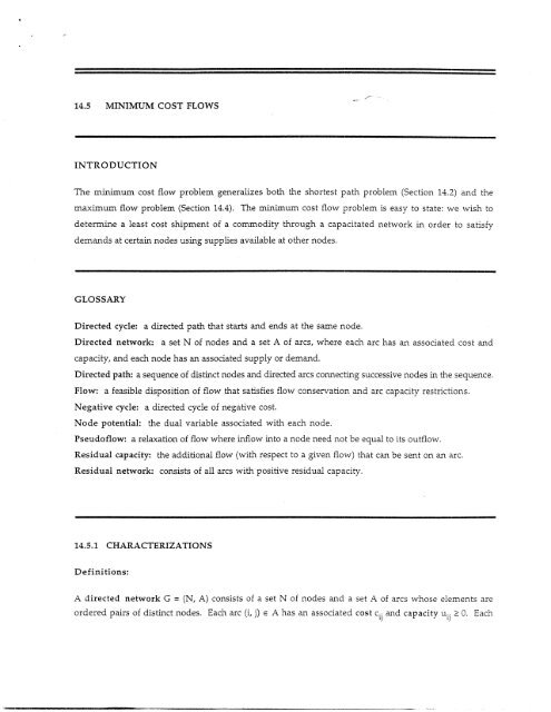
L I -1 I L L I __14.5 MINIMUM COST FLOWS· I I ·II .1 III r C I _I·C1311 -- -- 1_ 111~mwwxoINTRODUCTIONThe minimum cost flow problem generalizes both the shortest path problem (Section 14.2) and themaximum flow problem (Section 14.4). The minimum cost flow problem is easy to state: we wish todetermine a least cost shipment of a commodity through a capacitated network in order to satisfydemands at certain nodes using supplies available at other nodes.GLOSSARYDirected cycle: a directed path that starts and ends at the same node.Directed network: a set N of nodes and a set A of arcs, where each arc has an associated cost andcapacity, and each node has an associated supply or demand.Directed path: a sequence of distinct nodes and directed arcs connecting successive nodes in the sequence.Flow: a feasible disposition of flow that satisfies flow conservation and arc capacity restrictions.Negative cycle: a directed cycle of negative cost.Node potential: the dual variable associated with each node.Pseudoflow: a relaxation of flow where inflow into a node need not be equal to its outflow.Residual capacity: the additional flow (with respect to a given flow) that can be sent on an arc.Residual network: consists of all arcs with positive residual capacity.14.5.1 CHARACTERIZATIONSDefinitions:A directed network G = (N, A) consists of a set N of nodes and a set A of arcs whose elements areordered pairs of distinct nodes. Each arc (i, j) E A has an associated cost c and capacity u.j > 0. Each'r$gaaoBBOiipasaPsaaplprar·llslr . -I-·..i---1 -------

2node i E N has an associated supply/demand b(i). If b(i) > 0 then node i is a supply node; if b(i) < 0then node i is a demand node. Let n IN! I and m = A .A graph G' = (N', A') is a subgraph of G = (N, A) if N' c N and A' c A.The minimum cost flow problem is the following optimization problem:minimize Z ij Xij (1)(i,j)e Asubject toE X - xji =b(i) for all ie N, (2)fj:(isj)E A {j:(j,i)e A0 < xij < uij forall (i, j)e A, (3)where iE N b(i) = 0.A flow is any x = (xij) satisfying (2)-(3). It is assumed that the minimum cost flow problem possesses afeasible solution. As shown in Section 14.4.3, feasibility of the minimum cost flow problem can beascertained by solving a maximum flow problem.A pseudoflow is any x = (xij) satisfying (3). A pseudoflow may violate the mass balance constraints (2).For a given pseudoflow x, the imbalance of each node iN - {s, t} is defined ase(i) =b(i)+ E S xi;.{j:(j,i)e A} {j:(i,j)E A)A node with a positive imbalance is called an excess node, a node with a negative imbalance is calleda deficit node, and a node with zero imbalance is called a balanced node.The residual network G(x) corresponding to a flow (or a pseudoflow) x is defined in the followingmanner. Replace each arc (i, j) e A by two arcs (i, j) and (j, i). The arc (i, j) has cost cij and residualcapacity rij = uij - xij, and the arc (j, i) has cost -cij and residual capacity rji = xij. The residualnetwork consists only of arcs with positive residual capacity.A directed path in the graph G = (N, A) is a subgraph of G consisting of an (alternating) sequence ofnodes and arcs il-al-i 2 -a 2 - v. -ir -ar i-ir where ak = (ik, iki) e A for all I k • r-1 and no node isrepeated. A directed path is also denoted as i-i 2 - ...- i r . A directed cycle is a directed path ii2 ..-i together with the arc (ir, il). A directed cycle is also denoted as i-i? 2 - ...- ir-i 1 . A directed cycle Wfor which (ij)E cij < 0 is called a negative cycle.mrlB6s4PBBSIIIPIWLb·IBB·ls "-- ·r aCbCIIIIIDIC-rC

3The dual variable associated with the mass balance constraint at node i is denoted by cr(i) and isreferred to as the potential of node i. With respect to a given set of node potentials, the reduced costof an arc (i, j) in the residual network G(x) is denoted by c 7 = cij - z(i) + (j).Facts:1. Negative cycle optimality conditions. A feasible solution x is an optimal solution of theminimum cost flow problem if and only if the residual network G(x*) contains no negative cost (directed)cycle.2. Reduced cost optimality conditions. A feasible solution x* is an optimal solution of the minimumcost flow problem if and only some set of node potentials X satisfies c > 0 for every arc (i, j) in G(x*).ii3. Complementary slackness optimality conditions. A feasible solution x* is an optimal solution ofthe minimum cost flow problem if and only if there exists a set of node potentials t such that for everyarc (i, j) e A:(a) if cj >0, thenx* =0;(b) if0 < xU < u * then ~~~~~~ii = 0(c) if c < 0, then xi = ui-14.5.2 ALGORITHMS FOR MINIMUM COST FLOWSA wide variety of algorithms are available to solve the minimum cost flow problem. Brief descriptionsof the following three algorithms are presented in this section: (a) the cycle-canceling algorithm, (b)the successive shortest path algorithm, and (c) the network simplex algorithm. Detailed descriptionsof these as well as several other algorithms can be found in [AhEtal93].Cycle-Canceling AlgorithmThe cycle-canceling algorithm is an immediate consequence of the negative cycle optimality conditions(Fact 1, Section 14.5.1). The algorithm starts with a feasible flow and successively augments flow alongnegative cycles in the residual network until there is no negative cycle (see Algorithm 1).~~lPs ----r s a ~ a a ~ r a r r ~ a

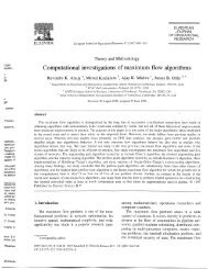
4.ALGORIThMC1 Cycnceling Algonthmalgoirithm yl-aclnestablish feaileflowt x the network Xn; :0: - -: ;: . .a : .- M. : :e k.... ,-,,while 0(x) containsanegative c;t~~~~~~~~' k m;1use.some algorithm tientf a eaieccle:-W`endend~~~~~~~~~~dtExample:1. Figure 1 illustrates the cycle-canceling algorithm. Figure (a) depicts the given flow network andalso gives a feasible flow in the network. Figure 1(b) shows the residual network. In the first iteration,suppose the algorithm selects the negative cycle 4-2-3-4 whose cost is -1. Then 6. = min{r 42, r 23 , r 34 } =min{3, 2, 41 = 2. The algorithm augments 2 units of flow along this cycle. Figure 1(c) shows the modifiedresidual network. In the next iteration, the algorithm selects the cycle 4-2-1-3-4 with cost -2 andaugments 1 unit of flow. Figure 1(d) depicts the updated residual network which contains no negativecycle; the algorithm terminates. From Figure 1(d), we deduce an optimal flow pattern of 2 units on arcs(1, 2), (1, 3), (2, 3) and 4 units on arc (3, 4).FIGURE 1Illustrating the cycle-canceling algorithm5jxii'i)(C rj)b(l) =4 b(4) = -4I / 1% Ib(3) = U(a)(b)·- -- 1~·---·1~-~- ~---·- · ----e -- III C. ~-e-----p ·I I- I II-

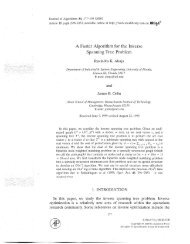
5(c)(d)Facts:1. A negative cycle in the residual network can be identified in O(nm) time by using a queueimplementation of the generic label-correcting algorithm (Fact 5, Section 14.2.2).2. Integrality property. For problems with integer arc capacities and integer node supplies/demands,the cycle-canceling algorithm starts with an integer solution and at each iteration augments by anintegral amount of flow. Consequently, the optimal solution produced by the algorithm is integer. Thisobservation implies that the minimum cost flow problem with integer supplies, demands, andcapacities always has an optimal solution which is integral.3. For problems with integer supplies, demands, and arc capacities, the generic version of the cyclecancelingalgorithm runs in pseudopolynomial time. If flow is augmented along a negative cycle W inG(x) that minimizes T(i j) W cij/IWI among all directed cycles in G(x), then this implementation runsin polynomial time [GoTa88].Successive Shortest Path AlgorithmThe successive shortest path algorithm starts with the pseudoflow x = 0. It proceeds by selecting anexcess node k, selecting a deficit node 1, and augmenting flow along a minimum cost path from node k tonode in G(x). The algorithm terminates when the network contains no excess or deficit nodes (seeAlgorithm 2)."lrllA~eII~B~31,1PRIMMMIRM-11 I_ _

77. Several implementations of the shortest augmenting path algorithm run in polynomial or evenstrongly polynomial time. [r88] describes an implementation running in O(m log n(m + n log n)) time,currently the fastest strongly polynomial-time algorithm to solve the minimum cost flow problem.FIGURE 2Illustrating the successive shortest path algorithme(i)Qa(cij' rij)e(j)6>,r4-42-2

8current spanning tree solution nto an improved spanning tee solution until optimality is reached (seeAlgorithm 3).Facts:8. Using tree data structures, the network simplex algorithm can be implemented very efficiently. Thenetwork simplex algorithm is one of the fastest algorithms to solve the minimum cost flow problem inpractice.9. The generic version of the network simplex algorithm has a exponential worst-case bound. [r95has recently suggested the first polynomial-time implementations of the (generic) network simplexalgorithm.14.5.3 APPLICATIONSMinimum cost flow problems arise in many industrial settings as well as many scientific domains. Someof the common applications of the minimum cost flow problem are: the distribution of a product frommanufacturing plants to warehouses, or from warehouses to retailers; the flow of raw materials andintermediate goods through various machining stations in a production line; the routing of automobilesthrough an urban street network; and the routing of calls through a telephone system. The minimumcost flow problem also has less transparent applications, including the three applications presentednext. [AhEtal93] present many additional applications of the minimum cost flow problem.jP.slll"'·--"----ap- --··l-···-CI-----·--a--- · _- IIC---·C---·IIII I--- -r ·9C '--------- --~--- ---- e

91. Leveling Mountainous TerrainA common problem facing civil engineers, when they are building road networks through hilly ormountainous terrain, is the distribution of earth from high points to low points of the terrain to producea leveled roadbed. The engineer must determine a plan for leveling the route by specifying the numberof truckloads of earth to move between various locations along the proposed road network.We first construct a terrain graphi: it is an undirected graph whose nodes represent locations with ademand for earth (low points) or locations with a supply of earth (high points). An arc of this graphrepresents an available route for distributing the earth, and the cost of this arc represents the cost pertruckload of moving earth between the corresponding two locations. Figure 1 shows a portion of asample terrain graph. A leveling plan for a terrain graph is a flow (set of truckloads) that meets thedemands at nodes (levels the low points) by the available supplies (earth obtained from high points)at the minimum cost for the truck movements. This model is a minimum cost flow problem defined onthe terrain graph.FIGURE 1Portion of a terrain graph2. Directed Chinese Postman ProblemLeaving from the post office, a postman needs to visit each house on each block in his postal route,delivering and collecting letters, and then return to the post office. The carrier would like to cover thisroute by traveling the minimum possible distance. In this version of the problem, known as thedirected Chinese postman problem, we assume that each street is directed. Mathematically, thisproblem is defined on a directed network G = (N, A) whose arcs (i j) have an associated nonnegative~~ - - -- - - -C-- · -"·-- I b- · ·

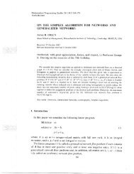
i:10length c. We wish to identify a directed alk (i.e., a sequence of nodes and arcs, not necessarilydistinct) of minimum length that starts at some node (the post office), visits each arc of the network atleast once, and returns to the starting node. In an optimal walk, a postman might traverse arcs morethan once. If xij denotes the number of times the postman traverses arc (i, j) in a walk, then this problemcan be formulated as:subject tomininmizeI Ai j Xij,(i,j)e Ax - xji =0 foral i N,{j:(i,j)e A} {j:(j,i)e Axij > 1 for all (i, j) A.This problem is a minor variant of the minimum cost flow problem where each arc has a lower bound ofone unit of flow. From an optimal flow x* of this problem, one can construct an optimal tour in thefollowing manner. First, replace each arc (i, j) with xj copies of the arc, each carrying a unit flow.Next, decompose the resulting network into a set of directed cycles. Finally, connect the directed cyclesto form a closed walk.3. Optimal Loading of a Hopping AirplaneA small commuter airline uses a plane with a capacity to carry at most p passengers on a "hoppingflight, as shown in Figure 2(a). The hopping flight visits the cities 1, 2, 3, ..., n, in a fixed sequence.The plane can pick up passengers at any city and drop them off at any other city. Let bij denote thenumber of passengers available at city i who want to go to city , and let f denote the fare per passengerfrom city i to city j. The airline would like to determine the number of passengers that the plane shouldcarry between various origins and destinations in order to maximize the total fare per trip while neverexceeding the plane's capacity.Figure 2(b) shows a minimum cost flow formulation of this hopping plane flight problem. The networkdisplays data only for those arcs with nonzero cost or finite capacity. Any arc without a displayed costhas zero cost; any arc without a displayed capacity has infinite capacity. For example, three types ofpassengers are available at node 1, those whose destination is node 2, node 3, or node 4. These threetypes of passengers are represented by the nodes 1-2, 1-3, and 14 with supplies b 12 , b , and b. Apassenger available at any such node, say 1-3, either boards the plane at its origin node by flowingthrough the arc (1-3, 1), and thus incurring a cost of -f 13 units, or never boards the plane, represented by

11flowing through the arc (1-3, 3). The feasible solutions for the minimum cost flow model correspond in aone-to-one manner with the feasible solutions for the hopping plane problem.FIGURE 2Formulation of the hopping airplane problem(a)b(i) cj or i b(j)G~~~~~~~~~~~~~~A- CiJo~uicosti- b 3 4(b)Q·C%161116(·i00;.·L·------c--C---- ---C-- - - L7 - -- ------·-L-·---·s-a_---·ao---a.- ---------- --- --- ---- II--- ---- I-I-___

12· · · I · I · --- L s-- __REFERENCES[AhEtal93]R. K. Ahuja, T. L. Magnanti, and . B. Orlin, Network Flows Theory, Algorithms, andApplications, Prentice-Hall, Englewood Cliffs, NJ, 1993.[Or88] J. B. Orlin, "A faster strongly polynomial minimum cost flow algorithm", Proceedings of the 20thACM Symposiutm on the Theory of Computing, 377-387, 1988. Full paper in Operations Research, 41(1993), 338-350.[GoTa88] A V. Goldberg and R. E. Tarjan, Finding minimum-cost circulations by canceling negativecycles", Proceedings of the 20th ACM Symposium on the Theory of Comptiting, pp. 7-18, 1988. Full paperin Journal of the ACM, 36(1989), 873-886.[0r95 J. B. Orlin, "A polynomial time primal network simplex algorithm for minimum cost flows",Technical Report, Sloan School of Management, MIT, Cambridge, MA, 1995.I L I · I I I L I _1- _ - _,,, sl- ^-·---·L--··C------.r I-- I -·s-1C;a54JrZ8ilgFP··CiaFi(allPI--- .- LI I --------- ------ ·--DI --·- L·-CI-·C· ··-·-····-·-----LI-· -- -* - _