Lectures on Modular Forms and Hecke Operators - William Stein

<strong>Lectures</strong> on Modular Forms and Hecke OperatorsKenneth A. RibetWilliam A. SteinOctober 5, 2011

ContentsPreface . . . . . . . . . . . . . . . . . . . . . . . . . . . . . . . . . . . . 11 The Main Objects 31.1 Torsion points on elliptic curves . . . . . . . . . . . . . . . . . . . . 31.1.1 The Tate module . . . . . . . . . . . . . . . . . . . . . . . . 31.2 Galois representations . . . . . . . . . . . . . . . . . . . . . . . . . 41.3 Modular forms . . . . . . . . . . . . . . . . . . . . . . . . . . . . . 51.4 Hecke operators . . . . . . . . . . . . . . . . . . . . . . . . . . . . . 62 Modular Representations and Algebraic Curves 72.1 Modular forms and Arithmetic . . . . . . . . . . . . . . . . . . . . 72.2 Characters . . . . . . . . . . . . . . . . . . . . . . . . . . . . . . . . 82.3 Parity conditions . . . . . . . . . . . . . . . . . . . . . . . . . . . . 92.4 Conjectures of Serre (mod l version) . . . . . . . . . . . . . . . . . 92.5 General remarks on mod p Galois representations . . . . . . . . . . 102.6 Serre’s conjecture . . . . . . . . . . . . . . . . . . . . . . . . . . . . 102.7 Wiles’s perspective . . . . . . . . . . . . . . . . . . . . . . . . . . . 113 Modular Forms of Level 1 133.1 The Definition . . . . . . . . . . . . . . . . . . . . . . . . . . . . . 133.2 Some examples and conjectures . . . . . . . . . . . . . . . . . . . . 143.3 Modular forms as functions on lattices . . . . . . . . . . . . . . . . 153.4 Hecke operators . . . . . . . . . . . . . . . . . . . . . . . . . . . . . 173.5 Hecke operators directly on q-expansions . . . . . . . . . . . . . . . 183.5.1 Explicit description of sublattices . . . . . . . . . . . . . . . 183.5.2 Hecke operators on q-expansions . . . . . . . . . . . . . . . 193.5.3 The Hecke algebra and eigenforms . . . . . . . . . . . . . . 213.5.4 Examples . . . . . . . . . . . . . . . . . . . . . . . . . . . . 213.6 Two Conjectures about Hecke operators on level 1 modular forms . 22

ivContents3.6.1 Maeda’s conjecture . . . . . . . . . . . . . . . . . . . . . . . 223.6.2 The Gouvea-Mazur conjecture . . . . . . . . . . . . . . . . 223.7 An Algorithm for computing characteristic polynomials of Heckeoperators . . . . . . . . . . . . . . . . . . . . . . . . . . . . . . . . 243.7.1 Review of basic facts about modular forms . . . . . . . . . 243.7.2 The Naive approach . . . . . . . . . . . . . . . . . . . . . . 253.7.3 The Eigenform method . . . . . . . . . . . . . . . . . . . . 253.7.4 How to write down an eigenvector over an extension field . 273.7.5 Simple example: weight 36, p = 3 . . . . . . . . . . . . . . . 284 Duality, Rationality, and Integrality 294.1 Modular forms for SL 2 (Z) and Eisenstein series . . . . . . . . . . . 294.2 Inner product . . . . . . . . . . . . . . . . . . . . . . . . . . . . . . 304.3 Eigenforms . . . . . . . . . . . . . . . . . . . . . . . . . . . . . . . 314.4 Integrality . . . . . . . . . . . . . . . . . . . . . . . . . . . . . . . . 314.5 A Result from Victor Miller’s thesis . . . . . . . . . . . . . . . . . 324.6 The Petersson inner product . . . . . . . . . . . . . . . . . . . . . 335 Analytic Theory of Modular Curves 375.1 The Modular group . . . . . . . . . . . . . . . . . . . . . . . . . . . 375.1.1 The Upper half plane . . . . . . . . . . . . . . . . . . . . . 375.2 Points on modular curves parameterize elliptic curves with extrastructure . . . . . . . . . . . . . . . . . . . . . . . . . . . . . . . . . 385.3 The Genus of X(N) . . . . . . . . . . . . . . . . . . . . . . . . . . 416 Modular Curves 456.1 Cusp Forms . . . . . . . . . . . . . . . . . . . . . . . . . . . . . . . 456.2 Modular curves . . . . . . . . . . . . . . . . . . . . . . . . . . . . . 466.3 Classifying Γ(N)-structures . . . . . . . . . . . . . . . . . . . . . . 466.4 More on integral Hecke operators . . . . . . . . . . . . . . . . . . . 476.5 Complex conjugation . . . . . . . . . . . . . . . . . . . . . . . . . . 476.6 Isomorphism in the real case . . . . . . . . . . . . . . . . . . . . . 476.7 The Eichler-Shimura isomorphism . . . . . . . . . . . . . . . . . . 486.8 The Petterson inner product is Hecke compatible . . . . . . . . . . 497 Modular Symbols 517.1 Modular symbols . . . . . . . . . . . . . . . . . . . . . . . . . . . . 517.2 Manin symbols . . . . . . . . . . . . . . . . . . . . . . . . . . . . . 527.2.1 Using continued fractions to obtain surjectivity . . . . . . . 537.2.2 Triangulating X(G) to obtain injectivity . . . . . . . . . . . 547.3 Hecke operators . . . . . . . . . . . . . . . . . . . . . . . . . . . . . 577.4 Modular symbols and rational homology . . . . . . . . . . . . . . . 587.5 Special values of L-functions . . . . . . . . . . . . . . . . . . . . . . 598 Modular Forms of Higher Level 638.1 Modular Forms on Γ 1 (N) . . . . . . . . . . . . . . . . . . . . . . . 638.2 The Diamond bracket and Hecke operators . . . . . . . . . . . . . 648.2.1 Diamond bracket operators . . . . . . . . . . . . . . . . . . 648.2.2 Hecke Operators on q-expansions . . . . . . . . . . . . . . . 668.3 Old and new subspaces . . . . . . . . . . . . . . . . . . . . . . . . . 66

Contentsv9 Newforms and Euler Products 699.1 Atkin-Lehner-Li theory . . . . . . . . . . . . . . . . . . . . . . . . 699.2 The U p operator . . . . . . . . . . . . . . . . . . . . . . . . . . . . 739.2.1 A Connection with Galois representations . . . . . . . . . . 749.2.2 When is U p semisimple? . . . . . . . . . . . . . . . . . . . . 759.2.3 An Example of non-semisimple U p . . . . . . . . . . . . . . 759.3 The Cusp forms are free of rank one over T C . . . . . . . . . . . . 759.3.1 Level 1 . . . . . . . . . . . . . . . . . . . . . . . . . . . . . 759.3.2 General level . . . . . . . . . . . . . . . . . . . . . . . . . . 779.4 Decomposing the anemic Hecke algebra . . . . . . . . . . . . . . . 7810 Some Explicit Genus Computations 8110.1 Computing the dimension of S k (Γ) . . . . . . . . . . . . . . . . . . 8110.2 Application of Riemann-Hurwitz . . . . . . . . . . . . . . . . . . . 8210.3 Explicit genus computations . . . . . . . . . . . . . . . . . . . . . . 8310.4 The Genus of X(N) . . . . . . . . . . . . . . . . . . . . . . . . . . 8310.5 The Genus of X 0 (N) . . . . . . . . . . . . . . . . . . . . . . . . . . 8310.6 Modular forms mod p . . . . . . . . . . . . . . . . . . . . . . . . . 8411 The Field of Moduli 8711.1 Digression on moduli . . . . . . . . . . . . . . . . . . . . . . . . . . 8811.2 When is ρ E surjective? . . . . . . . . . . . . . . . . . . . . . . . . . 8811.3 Observations . . . . . . . . . . . . . . . . . . . . . . . . . . . . . . 8911.4 A descent problem . . . . . . . . . . . . . . . . . . . . . . . . . . . 9011.5 Second look at the descent exercise . . . . . . . . . . . . . . . . . . 9111.6 Action of GL 2 . . . . . . . . . . . . . . . . . . . . . . . . . . . . . . 9212 Hecke Operators as Correspondences 9512.1 The Definition . . . . . . . . . . . . . . . . . . . . . . . . . . . . . 9512.2 Maps induced by correspondences . . . . . . . . . . . . . . . . . . . 9712.3 Induced maps on Jacobians of curves . . . . . . . . . . . . . . . . . 9812.4 More on Hecke operators . . . . . . . . . . . . . . . . . . . . . . . . 9912.5 Hecke operators acting on Jacobians . . . . . . . . . . . . . . . . . 9912.5.1 The Albanese Map . . . . . . . . . . . . . . . . . . . . . . . 10012.5.2 The Hecke algebra . . . . . . . . . . . . . . . . . . . . . . . 10112.6 The Eichler-Shimura relation . . . . . . . . . . . . . . . . . . . . . 10112.7 Applications of the Eichler-Shimura relation . . . . . . . . . . . . . 10512.7.1 The Characteristic polynomial of Frobenius . . . . . . . . . 10512.7.2 The Cardinality of J 0 (N)(F p ) . . . . . . . . . . . . . . . . . 10713 Abelian Varieties 10913.1 Abelian varieties . . . . . . . . . . . . . . . . . . . . . . . . . . . . 10913.2 Complex tori . . . . . . . . . . . . . . . . . . . . . . . . . . . . . . 11013.2.1 Homomorphisms . . . . . . . . . . . . . . . . . . . . . . . . 11013.2.2 Isogenies . . . . . . . . . . . . . . . . . . . . . . . . . . . . . 11213.2.3 Endomorphisms . . . . . . . . . . . . . . . . . . . . . . . . 11313.3 Abelian varieties as complex tori . . . . . . . . . . . . . . . . . . . 11313.3.1 Hermitian and Riemann forms . . . . . . . . . . . . . . . . 11413.3.2 Complements, quotients, and semisimplicity of the endomorphismalgebra . . . . . . . . . . . . . . . . . . . . . . . . . . 115

viContents13.3.3 Theta functions . . . . . . . . . . . . . . . . . . . . . . . . . 11713.4 A Summary of duality and polarizations . . . . . . . . . . . . . . . 11713.4.1 Sheaves . . . . . . . . . . . . . . . . . . . . . . . . . . . . . 11813.4.2 The Picard group . . . . . . . . . . . . . . . . . . . . . . . . 11813.4.3 The Dual as a complex torus . . . . . . . . . . . . . . . . . 11813.4.4 The Néron-Severi group and polarizations . . . . . . . . . . 11913.4.5 The Dual is functorial . . . . . . . . . . . . . . . . . . . . . 11913.5 Jacobians of curves . . . . . . . . . . . . . . . . . . . . . . . . . . . 11913.5.1 Divisors on curves and linear equivalence . . . . . . . . . . 12013.5.2 Algebraic definition of the Jacobian . . . . . . . . . . . . . 12113.5.3 The Abel-Jacobi theorem . . . . . . . . . . . . . . . . . . . 12213.5.4 Every abelian variety is a quotient of a Jacobian . . . . . . 12313.6 Néron models . . . . . . . . . . . . . . . . . . . . . . . . . . . . . . 12513.6.1 What are Néron models? . . . . . . . . . . . . . . . . . . . 12513.6.2 The Birch and Swinnerton-Dyer conjecture and Néron models12713.6.3 Functorial properties of Neron models . . . . . . . . . . . . 12914 Abelian Varieties Attached to Modular Forms 13114.1 Decomposition of the Hecke algebra . . . . . . . . . . . . . . . . . 13114.1.1 The Dimension of the algebras L f . . . . . . . . . . . . . . 13214.2 Decomposition of J 1 (N) . . . . . . . . . . . . . . . . . . . . . . . . 13314.2.1 Aside: intersections and congruences . . . . . . . . . . . . . 13414.3 Galois representations attached to A f . . . . . . . . . . . . . . . . 13514.3.1 The Weil pairing . . . . . . . . . . . . . . . . . . . . . . . . 13614.3.2 The Determinant . . . . . . . . . . . . . . . . . . . . . . . . 13814.4 Remarks about the modular polarization . . . . . . . . . . . . . . . 13915 Modularity of Abelian Varieties 14115.1 Modularity over Q . . . . . . . . . . . . . . . . . . . . . . . . . . . 14115.2 Modularity of elliptic curves over Q . . . . . . . . . . . . . . . . . 14415.3 Modularity of abelian varieties over Q . . . . . . . . . . . . . . . . 14416 L-functions 14716.1 L-functions attached to modular forms . . . . . . . . . . . . . . . . 14716.1.1 Analytic continuation and functional equations . . . . . . . 14816.1.2 A Conjecture about nonvanishing of L(f, k/2) . . . . . . . . 15016.1.3 Euler products . . . . . . . . . . . . . . . . . . . . . . . . . 15016.1.4 Visualizing L-function . . . . . . . . . . . . . . . . . . . . . 15117 The Birch and Swinnerton-Dyer Conjecture 15317.1 The Rank conjecture . . . . . . . . . . . . . . . . . . . . . . . . . . 15317.2 Refined rank zero conjecture . . . . . . . . . . . . . . . . . . . . . . 15517.2.1 The Number of real components . . . . . . . . . . . . . . . 15617.2.2 The Manin index . . . . . . . . . . . . . . . . . . . . . . . . 15617.2.3 The Real volume Ω A . . . . . . . . . . . . . . . . . . . . . . 15717.2.4 The Period mapping . . . . . . . . . . . . . . . . . . . . . . 15817.2.5 The Manin-Drinfeld theorem . . . . . . . . . . . . . . . . . 15817.2.6 The Period lattice . . . . . . . . . . . . . . . . . . . . . . . 15817.2.7 The Special value L(A, 1) . . . . . . . . . . . . . . . . . . . 15917.2.8 Rationality of L(A, 1)/Ω A . . . . . . . . . . . . . . . . . . . 159

Contentsvii17.3 General refined conjecture . . . . . . . . . . . . . . . . . . . . . . . 16117.4 The Conjecture for non-modular abelian varieties . . . . . . . . . . 16117.5 Visibility of Shafarevich-Tate groups . . . . . . . . . . . . . . . . . 16217.5.1 Definitions . . . . . . . . . . . . . . . . . . . . . . . . . . . 16317.5.2 Every element of H 1 (K, A) is visible somewhere . . . . . . . 16417.5.3 Visibility in the context of modularity . . . . . . . . . . . . 16417.5.4 Future directions . . . . . . . . . . . . . . . . . . . . . . . . 16617.6 Kolyvagin’s Euler system of Heegner points . . . . . . . . . . . . . 16717.6.1 A Heegner point when N = 11 . . . . . . . . . . . . . . . . 17617.6.2 Kolyvagin’s Euler system for curves of rank at least 2 . . . 17718 The Gorenstein Property for Hecke Algebras 17918.1 Mod l representations associated to modular forms . . . . . . . . . 17918.2 The Gorenstein property . . . . . . . . . . . . . . . . . . . . . . . . 18218.3 Proof of the Gorenstein property . . . . . . . . . . . . . . . . . . . 18418.3.1 Vague comments . . . . . . . . . . . . . . . . . . . . . . . . 18718.4 Finite flat group schemes . . . . . . . . . . . . . . . . . . . . . . . 18718.5 Reformulation of V = W problem . . . . . . . . . . . . . . . . . . . 18818.6 Dieudonné theory . . . . . . . . . . . . . . . . . . . . . . . . . . . . 18918.7 The proof: part II . . . . . . . . . . . . . . . . . . . . . . . . . . . 18918.8 Key result of Boston-Lenstra-Ribet . . . . . . . . . . . . . . . . . . 19219 Local Properties of ρ λ 19319.1 Definitions . . . . . . . . . . . . . . . . . . . . . . . . . . . . . . . . 19319.2 Local properties at primes p ∤ N . . . . . . . . . . . . . . . . . . . 19419.3 Weil-Deligne Groups . . . . . . . . . . . . . . . . . . . . . . . . . . 19419.4 Local properties at primes p | N . . . . . . . . . . . . . . . . . . . 19419.5 Definition of the reduced conductor . . . . . . . . . . . . . . . . . . 19520 Adelic Representations 19720.1 Adelic representations associated to modular forms . . . . . . . . . 19720.2 More local properties of the ρ λ . . . . . . . . . . . . . . . . . . . . . 20020.2.1 Possibilities for π p . . . . . . . . . . . . . . . . . . . . . . . 20120.2.2 The case l = p . . . . . . . . . . . . . . . . . . . . . . . . . 20220.2.3 Tate curves . . . . . . . . . . . . . . . . . . . . . . . . . . . 20321 Serre’s Conjecture 20521.1 The Family of λ-adic representations attached to a newform . . . . 20621.2 Serre’s Conjecture A . . . . . . . . . . . . . . . . . . . . . . . . . . 20621.2.1 The Field of definition of ρ . . . . . . . . . . . . . . . . . . 20721.3 Serre’s Conjecture B . . . . . . . . . . . . . . . . . . . . . . . . . . 20821.4 The Level . . . . . . . . . . . . . . . . . . . . . . . . . . . . . . . . 20821.4.1 Remark on the case N(ρ) = 1 . . . . . . . . . . . . . . . . . 20921.4.2 Remark on the proof of Conjecture B . . . . . . . . . . . . 21021.5 The Weight . . . . . . . . . . . . . . . . . . . . . . . . . . . . . . . 21121.5.1 The Weight modulo l − 1 . . . . . . . . . . . . . . . . . . . 21121.5.2 Tameness at l . . . . . . . . . . . . . . . . . . . . . . . . . . 21121.5.3 Fundamental characters of the tame extension . . . . . . . 21221.5.4 The Pair of characters associated to ρ . . . . . . . . . . . . 21321.5.5 Recipe for the weight . . . . . . . . . . . . . . . . . . . . . 214

viiiContents21.5.6 The World’s first view of fundamental characters . . . . . . 21521.5.7 Fontaine’s theorem . . . . . . . . . . . . . . . . . . . . . . . 21521.5.8 Guessing the weight (level 2 case) . . . . . . . . . . . . . . 21521.5.9 θ-cycles . . . . . . . . . . . . . . . . . . . . . . . . . . . . . 21621.5.10 Edixhoven’s paper . . . . . . . . . . . . . . . . . . . . . . . 21821.6 The Character . . . . . . . . . . . . . . . . . . . . . . . . . . . . . 21821.6.1 A Counterexample . . . . . . . . . . . . . . . . . . . . . . . 22021.7 The Weight revisited: level 1 case . . . . . . . . . . . . . . . . . . . 22121.7.1 Companion forms . . . . . . . . . . . . . . . . . . . . . . . . 22121.7.2 The Weight: the remaining level 1 case . . . . . . . . . . . . 22221.7.3 Finiteness . . . . . . . . . . . . . . . . . . . . . . . . . . . . 22322 Fermat’s Last Theorem 22522.1 The application to Fermat . . . . . . . . . . . . . . . . . . . . . . . 22522.2 Modular elliptic curves . . . . . . . . . . . . . . . . . . . . . . . . . 22723 Deformations 22923.1 Introduction . . . . . . . . . . . . . . . . . . . . . . . . . . . . . . . 22923.2 Condition (∗) . . . . . . . . . . . . . . . . . . . . . . . . . . . . . . 23023.2.1 Finite flat representations . . . . . . . . . . . . . . . . . . . 23123.3 Classes of liftings . . . . . . . . . . . . . . . . . . . . . . . . . . . . 23123.3.1 The case p ≠ l . . . . . . . . . . . . . . . . . . . . . . . . . 23123.3.2 The case p = l . . . . . . . . . . . . . . . . . . . . . . . . . 23223.4 Wiles’s Hecke algebra . . . . . . . . . . . . . . . . . . . . . . . . . 23324 The Hecke Algebra T Σ 23524.1 The Hecke algebra . . . . . . . . . . . . . . . . . . . . . . . . . . . 23524.2 The Maximal ideal in R . . . . . . . . . . . . . . . . . . . . . . . . 23724.2.1 Strip away certain Euler factors . . . . . . . . . . . . . . . . 23724.2.2 Make into an eigenform for U l . . . . . . . . . . . . . . . . 23824.3 The Galois representation . . . . . . . . . . . . . . . . . . . . . . . 23924.3.1 The Structure of T m . . . . . . . . . . . . . . . . . . . . . . 24024.3.2 The Philosophy in this picture . . . . . . . . . . . . . . . . 24024.3.3 Massage ρ . . . . . . . . . . . . . . . . . . . . . . . . . . . . 24024.3.4 Massage ρ ′ . . . . . . . . . . . . . . . . . . . . . . . . . . . 24124.3.5 Representations from modular forms mod l . . . . . . . . . 24224.3.6 Representations from modular forms mod l n . . . . . . . . 24224.4 ρ ′ is of type Σ . . . . . . . . . . . . . . . . . . . . . . . . . . . . . . 24324.5 Isomorphism between T m and R mR . . . . . . . . . . . . . . . . . . 24424.6 Deformations . . . . . . . . . . . . . . . . . . . . . . . . . . . . . . 24524.7 Wiles’s main conjecture . . . . . . . . . . . . . . . . . . . . . . . . 24624.8 T Σ is a complete intersection . . . . . . . . . . . . . . . . . . . . . 24824.9 The Inequality #O/η ≤ #℘ T /℘ 2 T ≤ #℘ R/℘ 2 R . . . . . . . . . . . . 24824.9.1 The Definitions of the ideals . . . . . . . . . . . . . . . . . . 24924.9.2 Aside: Selmer groups . . . . . . . . . . . . . . . . . . . . . . 25024.9.3 Outline of some proofs . . . . . . . . . . . . . . . . . . . . . 25025 Computing with Modular Forms and Abelian Varieties 25326 The Modular Curve X 0 (389) 255

Contentsix26.1 Factors of J 0 (389) . . . . . . . . . . . . . . . . . . . . . . . . . . . 25626.1.1 Newforms of level 389 . . . . . . . . . . . . . . . . . . . . . 25626.1.2 Isogeny structure . . . . . . . . . . . . . . . . . . . . . . . . 25726.1.3 Mordell-Weil ranks . . . . . . . . . . . . . . . . . . . . . . . 25726.2 The Hecke algebra . . . . . . . . . . . . . . . . . . . . . . . . . . . 25826.2.1 The Discriminant is divisible by p . . . . . . . . . . . . . . 25826.2.2 Congruences primes in S p+1 (Γ 0 (1)) . . . . . . . . . . . . . . 25926.3 Supersingular points in characteristic 389 . . . . . . . . . . . . . . 26026.3.1 The Supersingular j-invariants in characteristic 389 . . . . 26026.4 Miscellaneous . . . . . . . . . . . . . . . . . . . . . . . . . . . . . . 26026.4.1 The Shafarevich-Tate group . . . . . . . . . . . . . . . . . . 26026.4.2 Weierstrass points on X 0 + (p) . . . . . . . . . . . . . . . . . 26126.4.3 A Property of the plus part of the integral homology . . . . 26126.4.4 The Field generated by points of small prime order on anelliptic curve . . . . . . . . . . . . . . . . . . . . . . . . . . 261References 263

PrefaceThis book began when the second author typed notes for the first author’s 1996Berkeley course on modular forms with a view toward explaining some of the keyideas in Wiles’s celebrated proof of Fermat’s Last Theorem. The second authorthen expanded and rewrote the notes while teaching a course at Harvard in 2003on modular abelian varieties.The intended audience of this book is advanced graduate students and mathematicalresearchers. This book is more advanced than [LR11, Ste07, DS05], andat a relatively similar level to [DI95], though with more details. It should be substantiallymore accessible than a typical research paper in the area.Some things about how this book is (or will be!) fully “modern” in that it takesinto account:• The full modularity theorem.• The proof of the full Serre conjecture• Computational techniques (algorithms, Sage)Notation∼= an isomorphism≈ a noncanonical isomorphismAcknowledgementJoe Wetherell wrote the first version of Section 2.5.

2 ContentsContactKenneth A. Ribet (ribet@math.berkeley.edu)William A. Stein (wstein@gmail.com)

1The Main Objects1.1 Torsion points on elliptic curvesThe main geometric objects that we will study in this book are elliptic curves,which are curves of genus one equipped with a distinguished point. More generally,we consider certain algebraic curves of larger genus called modular curves, which inturn give rise via the Jacobian construction to higher-dimensional abelian varietiesfrom which we will obtain representations of the Galois group Gal(Q/Q) of therational numbers.It is convenient to view the group of complex points E(C) on an elliptic curve Eover the complex numbers C as a quotient C/L. Here{∫}L = ω : γ ∈ H 1 (E(C), Z)γis a lattice attached to a nonzero holomorphic differential ω on E, and the homologyH 1 (E(C), Z) ≈ Z×Z is the abelian group of smooth closed paths on E(C) modulothe homology relations.Viewing E as C/L immediately gives us information about the structure of thegroup of torsion points on E, which we exploit in the next section to constructtwo-dimensional representations of Gal(Q/Q).1.1.1 The Tate moduleIn the 1940s, Andre Weil studied the analogous situation for elliptic curves definedover a finite field k. He desperately wanted to find an algebraic way to describethe above relationship between elliptic curves and lattices. He found an algebraicdefinition of L/nL, when n is prime to the characteristic of k.LetE[n] := {P ∈ E(k) : nP = 0}.

4 1. The Main ObjectsWhen E is defined over C,( ) 1E[n] =n L /L ∼ = L/nL ≈ (Z/nZ) × (Z/nZ),so E[n] is a purely algebraic object canonically isomorphic to L/nL.Now suppose E is defined over an arbitrary field k. For any prime l, letE[l ∞ ] := {P ∈ E(k) : l ν P = 0, some ν ≥ 1}∞⋃= E[l ν ] = lim E[l ν ]. −→ν=1In an analogous way, Tate constructed a rank 2 free Z l -moduleT l (E) := lim ←−E[l ν ],where the map E[l ν ] → E[l ν−1 ] is multiplication by l. The Z/l ν Z-module structureof E[l ν ] is compatible with the maps E[l ν ] l −→ E[l ν−1 ] (see, e.g., [Sil92, III.7]).If l is coprime to the characteristic of the base field k, then T l (E) is free of rank 2over Z l , andV l (E) := T l (E) ⊗ Q lis a 2-dimensional vector space over Q l .1.2 Galois representationsNumber theory is largely concerned with the Galois group Gal(Q/Q), which isoften studied by considering continuous linear representationsρ : Gal(Q/Q) → GL n (K)where K is a field and n is a positive integer, usually 2 in this book. Artin, Shimura,Taniyama, and Tate pioneered the study of such representations.Let E be an elliptic curve defined over the rational numbers Q. Then Gal(Q/Q)acts on the set E[n], and this action respects the group operations, so we obtain arepresentationρ : Gal(Q/Q) → Aut(E[n]) ≈ GL 2 (Z/nZ).Let K be the field cut out by the ker(ρ), i.e., the fixed field of ker(ρ). Then K isa finite Galois extension of Q. SinceGal(K/Q) ∼ = Gal(Q/Q)/ ker ρ ∼ = Im ρ ↩→ GL 2 (Z/nZ)we obtain, in this way, subgroups of GL 2 (Z/nZ) as Galois groups.Shimura showed that if we start with the elliptic curve E defined by the equationy 2 + y = x 3 − x 2 then for “most” n the image of ρ is all of GL 2 (Z/nZ). Moregenerally, the image is “most” of GL 2 (Z/nZ) when E does not have complexmultiplication. (We say E has complex multiplication if its endomorphism ringover C is strictly larger than Z.)

1.3 Modular forms 51.3 Modular formsMany spectacular theorems and deep conjectures link Galois representations withmodular forms. Modular forms are extremely symmetric analytic objects, whichwe will first view as holomorphic functions on the complex upper half plane thatbehave well with respect to certain groups of transformations.Let SL 2 (Z) be the group of 2 × 2 integer matrices with determinant 1. For anypositive integer N, consider the subgroup{( )}a bΓ 1 (N) := ∈ SLc d 2 (Z) : a ≡ d ≡ 1, c ≡ 0 (mod N)( )1 ∗of matrices in SL 2 (Z) that are of the form when reduced modulo N.0 1The space S k (N) of cusp forms of weight k and level N for Γ 1 (N) consists ofall holomorphic functions f(z) on the complex upper half planeh = {z ∈ C : Im(z) > 0}that vanish at the cusps (see below) and satisfy the equation( )( )az + bf = (cz + d) k a bf(z) for all ∈ Γcz + dc d 1 (N) and z ∈ h.Thus f(z + 1) = f(z), so f determines a function F of q(z) = e 2πiz such thatF (q) = f(z). Viewing F as a function on {z : 0 < |z| < 1}, the condition thatf(z) is holomorphic and vanishes at infinity is that F (z) extends to a holomorphicfunction on {z : |z| < 1} and F (0) = 0. In this case, f is determined by its Fourierexpansion∞∑f(q) = a n q n .n=1It is also useful to consider the space M k (N) of modular forms of level N, whichis defined in the same way as S k (N), except that the condition that F (0) = 0 isrelaxed, and we require only that F extends to a holomorphic function at 0 (andthere is a similar condition at the cusps other than ∞).The spaces M k (N) and S k (N) are finite dimensional.Example 1.3.1. We compute dim(M 5 (30)) and dim(S 5 (30)) in Sage:sage : ModularForms ( Gamma1 (30) ,5). dimension ()112sage : CuspForms ( Gamma1 (30) ,5). dimension ()80For example, the space S 12 (1) has dimension one and is spanned by the famouscusp form∞∏∞∑∆ = q (1 − q n ) 24 = τ(n)q n .n=1The coefficients τ(n) define the Ramanujan τ-function. A non-obvious fact is that τis multiplicative and for every prime p and positive integer ν, we haven=1τ(p ν+1 ) = τ(p)τ(p ν ) − p 11 τ(p ν−1 ).

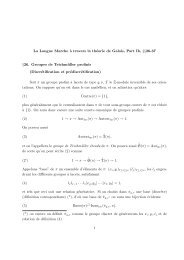
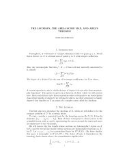
6 1. The Main ObjectsExample 1.3.2. We draw a plot of the ∆ function (using 20 terms of the q-expansion) on the upper half plane. Notice the symmetry ∆(z) = ∆(z + 1):0.70.60.50.40.30.20.1-2 -1.5 -1 -0.5 0.5 1 1.5 2sage : z = var (’z’); q = exp (2* pi*i*z)sage : D = delta_qexp (20)( q)sage : complex_plot (D, ( -2 ,2) , (0 ,.75) , plot_points =200)1.4 Hecke operatorsMordell defined operators T n , n ≥ 1, on S k (N) which are called Hecke operators.These proved very fruitful. The set of such operators forms a commuting family ofendomorphisms and is hence “almost” simultaneously diagonalizable.Often there is a basis f 1 , . . . , f r of S k (N) such that each f = f i = ∑ ∞n=1 a nq nis a simultaneous eigenvector for all the Hecke operators T n normalized so thatT n f = a n f, i.e., so the coefficient of q is 1. In this situation, the eigenvalues a n arenecessarily algebraic integers and the fieldK = K f = Q(. . . , a n , . . .)generated by all a n is finite over Q.The a n exhibit remarkable properties. For example,τ(n) ≡ ∑ d|nd 11 (mod 691).We can check this congruence for n = 30 in Sage as follows:sage : n =30; t = delta_qexp (n +1)[ n]; t-29211840sage : sigma (n ,11)17723450167663752sage : ( sigma (n ,11) - t )%6910The key to studying and interpreting the a n is to understand the deep connectionsbetween Galois representations and modular forms that were discovered bySerre, Shimura, Eichler and Deligne.

2Modular Representations and AlgebraicCurves2.1 Modular forms and ArithmeticConsider a cusp formf =∞∑a n q n ∈ S k (N)n=1which is an eigenform for all of the Hecke operators T p , and assume f is normalizedso a 1 = 1. Then the Mellin transform of f is the L-functionL(f, s) =∞∑n=1a nn s .Hecke proved that L(f, s) extends uniquely to a holomorphic function on C thatsatisfies a functional equation.Let K = Q(a 1 , a 2 , . . .) be the number field generated by the Fourier coefficientsof f. One can show that the a n are algebraic integers and that K is a number field.When k = 2, Shimura associated to f an abelian variety A f over Q of dimension[K : Q] on which Z[a 1 , a 2 , . . .] acts [Shi94, Theorem 7.14].Example 2.1.1 (Modular Elliptic Curves). Suppose now that all coefficients a n of flie in Q so that [K : Q] = 1 and hence A f is a one dimensional abelian variety, i.e.,an elliptic curve. An elliptic curve isogenous to one arising via this construction iscalled modular.Elliptic curves E 1 and E 2 are isogenous if there is a morphism E 1 → E 2 ofalgebraic groups, having finite kernel.The following theorem motivates much of the theory discussed in this course. Itis a theorem of Breuil, Conrad, Diamond, Taylor, and Wiles (see [BCDT01]).Theorem 2.1.2 (Modularity Theorem). Every elliptic curve over Q is modular,that is, isogenous to a curve constructed in the above way.

8 2. Modular Representations and Algebraic CurvesFor k ≥ 2 Serre and Deligne discovered a way to associate to f a family of l-adicrepresentations. Let l be a prime number and K = Q(a 1 , a 2 , . . .) be as above.Then it is well known that∏K ⊗ Q Q l∼ = K λ .One can associate to f a representationλ|lρ l,f : G = Gal(Q/Q) → GL 2 (K ⊗ Q Q l )unramified at all primes p ∤ lN. Let Z be the ring of all algebraic integers. For ρ l,fto be unramified at p we mean that for all primes P of Z lying over p, the inertiasubgroup of the decomposition group at P is contained in the kernel of ρ l,f . Thedecomposition group D P at P is the set of those g ∈ G which fix P . Let k bethe residue field Z/P and k = F p . Then the inertia group I P is the kernel of thesurjective map D P → Gal(k/k).Now I P ⊂ D P ⊂ Gal(Q/Q) and D P /I P is pro-cyclic (being isomorphic to theGalois group Gal(k/k)), so it is generated by a Frobenious automorphism Frob plying over p. One hastr(ρ l,f (Frob p )) = a p ∈ K ⊂ K ⊗ Q landdet(ρ l,f ) = χ k−1lεwhere, as explained below, χ l is the lth cyclotomic character and ε is the Dirichletcharacter associated to f.There is an incredible amount of “abuse of notation” packed into the abovestatement. Let M = Q ker(ρ l,f )be the field fixed by the kernel of ρl,f . Then theFrobenius element Frob P (note P not p) is well defined as an element of Gal(M/Q),and the element Frob p is then only well defined up to conjugacy. But this worksout since ρ l,f is well-defined on Gal(M/Q) (it kills Gal(Q/M)) and trace is welldefinedon conjugacy classes (tr(AB) = tr(BA) so tr(ABA −1 ) = T r(B)).2.2 CharactersLet f ∈ S k (N) be an eigenform for all Hecke operators. Then for all ( )a bc d ∈ SL2 (Z)with c ≡ 0 mod N we have( ) az + bf = (cz + d) k ε(d)f(z),cz + dwhere ε : (Z/NZ) ∗ → C ∗ is a Dirichlet character mod N. If f is also normalizedso that a 1 = 1, as in Section 1.4, then ε actually takes values in K ∗ .Let G = Gal(Q/Q), and let ϕ N be the mod N cyclotomic character so thatϕ N : G → (Z/NZ) ∗ takes g ∈ G to the automorphism induced by g on theNth cyclotomic extension Q(µ N ) of Q (where we identify Gal(Q(µ N )/Q) with(Z/NZ) ∗ ). Then what we called ε above in the formula det(ρ l ) = χ k−1lε is reallythe compositionG ϕ N−−→ (Z/NZ) ∗ ε−→ C ∗ .

2.3 Parity conditions 9For each positive integer ν we consider the l ν th cyclotomic character on G,ϕ l ν : G → (Z/l ν Z) ∗ .Putting these together gives the l-adic cyclotomic characterχ l : G → Z ∗ l .2.3 Parity conditionsLet c ∈ Gal(Q/Q) be complex conjugation. Then ϕ N (c) = −1 so ε(c) = ε(−1)and χ k−1l(c) = (−1) k−1 . Letting ( ) (a b = −1 0)0 −1 , for f ∈ Sk (N), we haveso (−1) k ε(−1) = 1. Thusc ′ df(z) = (−1) k ε(−1)f(z),det(ρ l,f (c)) = ε(−1)(−1) k−1 = −1.We say a representation is odd if the determinant of complex conjugation is −1.Thus the representation ρ l,f is odd.Remark 2.3.1 (Vague Question). How can one recognize representations like ρ l,f“in nature”? Fontaine and Mazur have made relevant conjectures. The modularitytheorem can be reformulated by saying that for any representation ρ l,E comingfrom an elliptic curve E there is an f so that ρ l,E∼ = ρl,f .2.4 Conjectures of Serre (mod l version)Suppose f is a modular form, l ∈ Z prime, λ a prime lying over l, and therepresentationρ λ,f : G → GL 2 (K λ )(constructed by Serre-Deligne) is irreducible. Then ρ λ,f is conjugate to a representationwith image in GL 2 (O λ ), where O λ is the ring of integers of K λ (seeSection 2.5 below). Reducing mod λ gives a representationρ λ,f : G → GL 2 (F λ )which has a well-defined trace and det, i.e., the det and trace do not depend onthe choice of conjugate representation used to obtain the reduced representation.One knows from representation theory (the Brauer-Nesbitt theorem – see [CR62])that if such a representation is semisimple then it is completely determined by itstrace and det (more precisely, it is determined by the characteristic polynomialsof all of its elements). Thus if ρ λ,f is irreducible (and hence semisimple) then it isunique in the sense that it does not depend on the choice of conjugate.

10 2. Modular Representations and Algebraic Curves2.5 General remarks on mod p Galois representationsFirst, what are semisimple and irreducible representations? Remember that a representationρ is a map from a group G to the endomorphisms of some vector spaceW (or a free module M if we are working over a ring instead of a field, but let’snot worry about that for now). A subspace W ′ of W is said to be invariant underρ if ρ takes W ′ back into itself. (The point is that if W ′ is invariant, then ρinduces representations on both W ′ and W/W ′ .) An irreducible representation isone whose only invariant subspaces are {0} and W . A semisimple representationis one where for every invariant subspace W ′ there is a complementary invariantsubspace W ′′ – that is, you can write ρ as the direct sum of ρ| W ′ and ρ| W ′′.Another way to say this is that if W ′ is an invariant subspace then we get ashort exact sequence0 → ρ| W/W ′ → ρ → ρ| W ′ → 0.Furthermore ρ is semisimple if and only if every such sequence splits.Note that irreducible representations are semisimple. As mentioned above, twodimensionalsemisimple Galois representations are uniquely determined (up to isomorphismclass) by their trace and determinant. In the case we are considering,G = Gal(Q/Q) is compact, so the image of any Galois representation ρ intoGL 2 (K λ ) is compact. Thus we can conjugate it into GL 2 (O λ ). Irreducibility is notneeded for this.Now that we have a representation into GL 2 (O λ ), we can reduce to get a representationρ to GL 2 (F λ ). This reduced representation is not uniquely determinedby ρ, since we made a choice of basis (via conjugation) so that ρ would have imagein GL 2 (O λ ), and a different choice may lead to a non-isomorphic representationmod λ. However, the trace and determinant of a matrix are invariant under conjugation,so the trace and determinant of the reduced representation ρ are uniquelydetermined by ρ.So we know the trace and determinant of the reduced representation. If we alsoknew that it was semisimple, then we would know its isomorphism class, and wewould be done. So we would be happy if the reduced representation is irreducible.And in fact, it is easy to see that if the reduced representation is irreducible, thenρ must also be irreducible. Most ρ of interest to us in this book will be irreducible.Unfortunately, the opposite implication does not hold: ρ irreducible need not implythat ρ is irreducible.2.6 Serre’s conjectureSerre has made the following conjecture which is now a theorem (see [KW08]).Conjecture 2.6.1 (Serre). All 2-dimensional irreducible representation of G overa finite field which are odd, i.e., det(σ(c)) = −1, c complex conjugation, are of theform ρ λ,f for some representation ρ λ,f constructed as above.Example 2.6.2. Let E/Q be an elliptic curve and let σ l : G → GL 2 (F l ) be therepresentation induced by the action of G on the l-torsion of E. Then det σ l = ϕ l isodd and σ l is usually irreducible, so Serre’s conjecture implies that σ l is modular.From this one can, assuming Serre’s conjecture, prove that E is itself modular (see[Rib92]).

2.7 Wiles’s perspective 11Definition 2.6.3 (Modular representation). Let σ : G → GL 2 (F) (F is a finitefield) be an irreducible representation of the Galois group G. Then we say thatthe representation σ is modular if there is a modular form f, a prime λ, and anembedding F ↩→ F λ such that σ ∼ = ρ λ,f over F λ .For more details, see Chapter 21 and [RS01].2.7 Wiles’s perspectiveSuppose E/Q is an elliptic curve and ρ l,E : G → GL 2 (Z l ) the associated l-adic representation on the Tate module T l . Then by reducing we obtain a mod lrepresentationρ l,E = σ l,E : G → GL 2 (F l ).If we can show this representation is modular for infinitely many l then we willknow that E is modular.Theorem 2.7.1 (Langlands and Tunnel). If σ 2,E and σ 3,E are irreducible, thenthey are modular.This is proved by using that GL 2 (F 2 ) and GL 2 (F 3 ) are solvable so we may applysomething called “base change for GL 2 .”Theorem 2.7.2 (Wiles). If ρ is an l-adic representation which is irreducible andmodular mod l with l > 2 and certain other reasonable hypothesis are satisfied,then ρ itself is modular.

12 2. Modular Representations and Algebraic Curves

3Modular Forms of Level 1In this chapter, we view modular forms of level 1 both as holomorphic functionson the upper half plane and functions on lattices. We then define Hecke operatorson modular forms, and derive explicit formulas for the action of Hecke operatorson q-expansions. An excellent reference for the theory of modular forms of level 1is Serre [Ser73, Ch. 7].3.1 The DefinitionLet k be an integer. The space S k = S k (1) of cusp forms of level 1 and weight kconsists of all functions f that are holomorphic on the upper half plane h and suchthat for all ( )a bc d ∈ SL2 (Z) one has( ) aτ + bf = (cτ + d) k f(τ), (3.1.1)cτ + dand f vanishes at infinity, in a sense which we will now make precise. The matrix( 1 0 11 ) is in SL 2(Z), so f(τ + 1) = f(τ). Thus f passes to a well-defined functionof q(τ) = e 2πiτ . Since for τ ∈ h we have |q(τ)| < 1, we may view f(z) = F (q) asa function of q on the punctured open unit disc {q : 0 < |q| < 1}. The conditionthat f(τ) vanishes at infinity means that F (q) extends to a holomorphic functionon the open disc {q : |q| < 1} so that F (0) = 0. Because holomorphic functionsare represented by power series, there is a neighborhood of 0 such thatf(q) =∞∑a n q n ,n=1so for all τ ∈ h with sufficiently large imaginary part (but see Remark 3.1.1 below),f(τ) = ∑ ∞n=1 a ne 2πinτ .

14 3. Modular Forms of Level 1It will also be useful to consider the slightly larger space M k (1) of holomorphicfunctions on h that transform as above and are merely required to be holomorphicat infinity.Remark 3.1.1. In fact, the series ∑ ∞n=1 a ne 2πinτ converges for all τ ∈ h. This isbecause the Fourier coefficients a n are O(n k/2 ) (see [Miy89, Cor. 2.1.6, pg. 43]).Remark 3.1.2. In [Ser73, Ch. 7], the weight is defined in the same way, but in thenotation our k is twice his k.3.2 Some examples and conjecturesThe space S k (1) of cusp forms is a finite-dimensional complex vector space. For keven we have dim S k (1) = ⌊k/12⌋ if k ≢ 2 (mod 12) and ⌊k/12⌋ − 1 if k ≡ 2(mod 12), except when k = 2 in which case the dimension is 0. For even k, thespace M k (1) has dimension 1 more than the dimension of S k (1), except when k = 2when both have dimension 0. (For proofs, see, e.g., [Ser73, Ch. 7, §3].)By the dimension formula mentioned above, the first interesting example is thespace S 12 (1), which is a 1-dimensional space spanned by∆(q) = q∞∏(1 − q n ) 24n=1= q − 24q 2 + 252q 3 − 1472q 4 + 4830q 5 − 6048q 6 − 16744q 7 + 84480q 8− 113643q 9 − 115920q 10 + 534612q 11 − 370944q 12 − 577738q 13 + · · ·That ∆ lies in S 12 (1) is proved in [Ser73, Ch. 7, §4.4] by expressing ∆ in termsof elements of M 4 (1) and M 6 (1), and computing the q-expansion of the resultingexpression.Example 3.2.1. We compute the q-expansion of ∆ in Sage:sage : delta_qexp (7)q - 24* q^2 + 252* q^3 - 1472* q^4 + 4830* q^5 - 6048* q^6 + O(q ^7)In Sage, computing delta_qexp(10^6) only takes a few seconds, and computing upto precision 10^8 is even reasonable. Sage does not use the formula q ∏ ∞n=1 (1−qn ) 24given above, which would take a very long time to directly evaluate, but insteaduses the identity⎛⎞∆(q) = ⎝ ∑ 8(−1) n (2n + 1)q n(n+1)/2 ⎠ ,n≥0and computes the 8th power using asymptotically fast polynomial arithmetic inZ[q], which involves a discrete fast Fourier transform (implemented in [HH]).The Ramanujan τ function τ(n) assigns to n the nth coefficient of ∆(q).Conjecture 3.2.2 (Lehmer). τ(n) ≠ 0 for all n ≥ 1.This conjecture has been verified for n ≤ 22798241520242687999 (Bosman, 2007– see http://en.wikipedia.org/wiki/Tau-function).

3.3 Modular forms as functions on lattices 15Theorem 3.2.3 (Edixhoven et al.). Let p be a prime. There is a polynomial timealgorithm to compute τ(p), polynomial in the number of digits of p.Edixhoven’s idea is to use l-adic cohomology and Arakelov theory to find ananalogue of the Schoof-Elkies-Atkin algorithm (which counts the number N q ofpoints on an elliptic curves over a finite field F q by computing N q mod l formany primes l). Here’s some of what Edixhoven has to say about his result:“You need to compute on varying curves such as X 1 (l) for l up tolog(p) say. An important by-product of my method is the computationof the mod l Galois representations associated to ∆ in time polynomialin l. So, it should be seen as an attempt to make the Langlandscorrespondence for GL 2 over Q available computationally.”If f ∈ M k (1) and g ∈ M k ′(1), then it is easy to see from the definitions thatfg ∈ M k+k ′(1). Moreover, ⊕ k≥0 M k(1) is a commutative graded ring generatedfreely by E 4 = 1+240 ∑ ∞n=1 σ 3(n)q n and E 6 = 1−504 ∑ ∞n=1 σ 5(n)q n , where σ d (n)is the sum of the dth powers of the positive divisors of n (see [Ser73, Ch.7, §3.2]).Example 3.2.4. Because E 4 and E 6 generate, it is straightforward to write downa basis for any space M k (1). For example, the space M 36 (1) has basisf 1 = 1 + 6218175600q 4 + 15281788354560q 5 + · · ·f 2 = q + 57093088q 4 + 37927345230q 5 + · · ·f 3 = q 2 + 194184q 4 + 7442432q 5 + · · ·f 4 = q 3 − 72q 4 + 2484q 5 + · · ·3.3 Modular forms as functions on latticesIn order to define Hecke operators, it will be useful to view modular forms asfunctions on lattices in C.Definition 3.3.1 (Lattice). A lattice L ⊂ C is a subgroup L = Zω 1 + Zω 2 forwhich ω 1 , ω 2 ∈ C are linearly independent over R.We may assume that ω 1 /ω 2 ∈ h = {z ∈ C : Im(z) > 0}. Let R be the set of alllattices in C. Let E be the set of isomorphism classes of pairs (E, ω), where E isan elliptic curve over C and ω ∈ Ω 1 E is a nonzero holomorphic differential 1-formon E. Two pairs (E, ω) and (E ′ , ω ′ ) are isomorphic if there is an isomorphismϕ : E → E ′ such that ϕ ∗ (ω ′ ) = ω.Proposition 3.3.2. There is a bijection between R and E under which L ∈ Rcorresponds to (C/L, dz) ∈ E.Proof. We describe the maps in each direction, but leave the proof that they inducea well-defined bijection as an exercise for the reader [[add ref to actual exercise]].Given L ∈ R, by Weierstrass theory the quotient C/L is an elliptic curve, which isequipped with the distinguished differential ω induced by the differential dz on C.Conversely, if E is an elliptic curve over C and ω ∈ Ω 1 E is a nonzero differential,we obtain a lattice L in C by integrating homology classes:{∫}L = L ω = ω : γ ∈ H 1 (E(C), Z) .γ

16 3. Modular Forms of Level 1LetB = {(ω 1 , ω 2 ) : ω 1 , ω 2 ∈ C, ω 1 /ω 2 ∈ h} ,be the set of ordered basis of lattices in C, ordered so that ω 1 /ω 2 ∈ h. There is aleft action of SL 2 (Z) on B given by( a bc d)(ω1 , ω 2 ) ↦→ (aω 1 + bω 2 , cω 1 + dω 2 )and SL 2 (Z)\B ∼ = R. (The action is just the left action of matrices on columnvectors, except we write (ω 1 , ω 2 ) as a row vector since it takes less space.)Give a modular form f ∈ M k (1), associate to f a function F : R → C as follows.First, on lattices of the special form Zτ + Z, for τ ∈ h, let F (Zτ + Z) = f(τ).In order to extend F to a function on all lattices, note that F satisfies thehomogeneity condition F (λL) = λ −k F (L), for any λ ∈ C and L ∈ R. ThenF (Zω 1 + Zω 2 ) = ω −k2 F (Zω 1/ω 2 + Z) := ω −k2 f(ω 1/ω 2 ).That F is well-defined exactly amounts to the transformation condition (3.1.1)that f satisfies.Lemma 3.3.3. The lattice function F : R → C associated to f ∈ M k (1) is welldefined.Proof. Suppose Zω 1 + Zω 2 = Zω 1 ′ + Zω 2 ′ with ω 1 /ω 2 and ω 1/ω ′ 2 ′ both in h. Wemust verify that ω2 −k f(ω 1/ω 2 ) = (ω 2) ′ −k f(ω 1/ω ′ 2). ′ There exists ( )a bc d ∈ SL2 (Z)such ( that ω 1 ′ = aω 1 + bω 2 and ω 2 ′ = cω 1 + dω 2 . Dividing, we see that ω 1/ω ′ 2 ′ =a b)c d (ω1 /ω 2 ). Because f is a weight k modular form, we have( ) (( ) ( )) (ω′f 1 a b ω1= f= c ω ) k ( )1 ω1+ d f .c d ω 2 ω 2 ω 2ω ′ 2Multiplying both sides by ω2 k yields( ) ωω2 k ′f 1= (cω 1 + dω 2 ) k fω ′ 2(ω1ω 2).Observing that ω ′ 2 = cω 1 + dω 2 and dividing again completes the proof.Since f(τ) = F (Zτ +Z), we can recover f from F , so the map f ↦→ F is injective.Moreover, it is surjective in the sense that if F is homogeneous of degree −k, thenF arises from a function f : h → C that transforms like a modular form. Moreprecisely, if F : R → C satisfies the homogeneity condition F (λL) = λ −k F (L),then the function f : h → C defined by f(τ) = F (Zτ +Z) transforms like a modularform of weight k, as the following computation shows: For any ( )a bc d ∈ SL2 (Z) andτ ∈ h, we havef( ) (aτ + b= F Z aτ + b )cτ + d cτ + d + Z= F ((cτ + d) −1 (Z(aτ + b) + Z(cτ + d)))= (cτ + d) k F (Z(aτ + b) + Z(cτ + d))= (cτ + d) k F (Zτ + Z)= (cτ + d) k f(τ).

3.4 Hecke operators 17Say that a function F : R → C is holomorphic on h ∪ {∞} if the function f(τ) =F (Zτ + Z) is. We summarize the above discussion in a proposition.Proposition 3.3.4. There is a bijection between M k (1) and functions F : R →C that are homogeneous of degree −k and holomorphic on h ∪ {∞}. Under thisbijection F : R → C corresponds to f(τ) = F (Zτ + Z).3.4 Hecke operatorsDefine a map T n from the free abelian group generated by all C-lattices into itselfbyT n (L) =∑ L ′ ⊂L[L:L ′ ]=nwhere the sum is over all sublattices L ′ ⊂ L of index n. For any function F : R → Con lattices, define T n (F ) : R → C by(T n (F ))(L) = n k−1 ∑L ′ ,L ′ ⊂L[L:L ′ ]=nF (L ′ ).If F is homogeneous of degree −k, then T n (F ) is also homogeneous of degree −k.We will next show that (n, m) = 1 implies T n T m = T nm and T p k is a polynomialin Z[T p ] (see [Ser73, Cor. 1, pg. 99]); the essential case to consider is n prime.Suppose L ′ ⊂ L with [L : L ′ ] = n. Then every element of L/L ′ has orderdividing n, so nL ⊂ L ′ ⊂ L andL ′ /nL ⊂ L/nL ≈ (Z/nZ) 2 .Thus the subgroups of (Z/nZ) 2 of order n correspond to the sublattices L ′ of L ofindex n. When n = l is prime, there are l + 1 such subgroups, since the subgroupscorrespond to nonzero vectors in F l modulo scalar equivalence, and there are(l 2 − 1)/(l − 1) = l + 1 of them.Recall from Proposition 3.3.2 that there is a bijection between the set R oflattices in C and the set E of isomorphism classes of pairs (E, ω), where E is anelliptic curve over C and ω is a nonzero differential on E.Suppose F : R → C is homogeneous of degree −k, so F (λL) = λ −k F (L). Thenwe may also view T l as a sum over lattices that contain L with index l, as follows.Suppose L ′ ⊂ L is a sublattice of index l and set L ′′ = l −1 L ′ . Then we have achain of inclusionslL ⊂ L ′ ⊂ L ⊂ l −1 L ′ = L ′′ .Since [l −1 L ′ : L ′ ] = l 2 and [L : L ′ ] = l, it follows that [L ′′ : L] = l. Because F ishomogeneous of degree −k,T l (F )(L) = l k−1∑[L:L ′ ]=lF (L ′ ) = 1 l∑[L ′′ :L]=lF (L ′′ ). (3.4.1)

18 3. Modular Forms of Level 13.5 Hecke operators directly on q-expansionsRecall that the nth Hecke operator T n of weight k on the free abelian group onlattices is given by∑T n (L) = n k−1 L ′ .L ′ ⊂L[L:L ′ ]=nModular forms of weight k correspond to holomorphic functions of degree −k onlattices, and each T n extends to an operator on these functions on lattices, so T ndefines on operator on M k (1).A holomorphic function on the unit disk is determined by its Fourier expansion,so Fourier expansion defines an injective map M k (1) ↩→ C[[q]]. In this section, wedescribe T n ( ∑ a m q m ) explicitly as a q-expansion.3.5.1 Explicit description of sublatticesIn order to describe T n more explicitly, we enumerate the sublattices L ′ ⊂ L ofindex n. More precisely, we give a basis for each L ′ in terms of a basis for L. Notethat L/L ′ is a group of order n andL ′ /nL ⊂ L/nL = (Z/nZ) 2 .Write L = Zω 1 + Zω 2 , let Y 2 be the cyclic subgroup of L/L ′ generated by ω 2 andlet d = #Y 2 . If Y 1 = (L/L ′ )/Y 2 , then Y 1 is generated by the image of ω 1 , so it is acyclic group of order a = n/d. Our goal is to exhibit a basis of L ′ . Let ω 2 ′ = dω 2 ∈ L ′and use that Y 1 is generated by the image of ω 1 to write aω 1 = ω 1 ′ − bω 2 for someinteger b and some ω 1 ′ ∈ L ′ . Since b is only well-defined modulo d we may assume0 ≤ b ≤ d − 1. Thus( ω′ ) (1 a b)( ω1)=0 d ω 2and the change of basis matrix has determinant ad = n. Sinceω ′ 2Zω ′ 1 + Zω ′ 2 ⊂ L ′ ⊂ L = Zω 1 + Zω 2and [L : Zω ′ 1 + Zω ′ 2] = n (since the change of basis matrix has determinant n) and[L : L ′ ] = n we see that L ′ = Zω ′ 1 + Zω ′ 2.Proposition 3.5.1. Let n be a positive integer. There is a one-to-one correspondencebetween sublattices L ′ ⊂ L of index n and matrices ( )a b0 d with ad = n and0 ≤ b ≤ d − 1.Proof. The correspondence is described above. To check that it is a bijection, wejust need to show that if γ = ( )a b0 d and γ ′ = ( )a ′ b ′0 d are two matrices satisfying′the listed conditions, andZ(aω 1 + bω 2 ) + Zdω 2 = Z(aω ′ 1 + bω ′ 2) + Zdω ′ 2,then γ = γ ′ . Equivalently, if σ ∈ SL 2 (Z) and σγ = γ ′ , then σ = 1. To see this, wecomputeσ = γ ′ γ −1 = 1 ( )a ′ d ab ′ − a ′ bn 0 ad ′ .

3.5 Hecke operators directly on q-expansions 19Since σ ∈ SL 2 (Z), we have n | a ′ d, and n | ad ′ , and aa ′ dd ′ = n 2 . If a ′ d > n, thenbecause aa ′ dd ′ = n 2 , we would have ad ′ < n, which would contradict the factthat n | ad ′ ; also, a ′ d < n is impossible since n | a ′ d. Thus a ′ d = n and likewisead ′ = n. Since ad = n as well, it follows that a ′ = a and d ′ = d, so σ = ( 1 0 1 t ) forsome t ∈ Z. Then σγ = ( )a b+dt0 d , which implies that t = 0, since 0 ≤ b ≤ d − 1and 0 ≤ b + dt ≤ d − 1.Remark 3.5.2. As mentioned earlier, when n = l is prime, there are l+1 sublatticesof index l. In general, the number of such sublattices is the sum of the positivedivisors of n (exercise) 1 . 13.5.2 Hecke operators on q-expansionsRecall that if f ∈ M k (1), then f is a holomorphic function on h ∪ {∞} such thatf(τ) = f( ) aτ + b(cτ + d) −kcτ + dfor all ( a bc d)∈ SL2 (Z). Using Fourier expansion we write∞∑f(τ) = c m e 2πiτm ,m=0and say f is a cusp form if c 0 = 0. Also, there is a bijection between modularforms f of weight k and holomorphic lattice functions F : R → C that satisfyF (λL) = λ −k F (L); under this bijection F corresponds to f(τ) = F (Zτ + Z).Now assume f(τ) = ∑ ∞m=0 c mq m is a modular form with corresponding latticefunction F . Using the explicit description of sublattices from Section 3.5.1 above,we can describe the action of the Hecke operator T n on the Fourier expansion of1 Put reference to actual exercise

20 3. Modular Forms of Level 1f(τ), as follows:T n F (Zτ + Z) = n k−1∑a,b,dad=n0≤b≤d−1F ((aτ + b)Z + dZ)= n ∑ ( aτ + bk−1 d −k Fd= n ∑ ( ) aτ + bk−1 d −k fd∑= n k−1a,d,b,m= n k−1 ∑a,d,m)Z + Zd −k aτ+bc m e2πi( d )md 1−k c m e 2πiamτd1d= n ∑ k−1 d 1−k c dm ′e 2πiam′ τad=nm ′ ≥0= ∑a k−1 c dm ′q am′ .ad=nm ′ ≥0∑d−1(b=0e 2πimdIn the second to the last expression we let m = dm ′ for m ′ ≥ 0, then use that thesum 1 ∑ d−1 2πimd b=0(e d ) b is only nonzero if d | m, in which case the sum equals 1.ThusT n f(q) = ∑a k−1 c dm q am .ad=nm≥0Put another way, if µ is a nonnegative integer, then the coefficient of q µ is∑a|na|µa k−1 c nµa 2 .(To see this, let m = a/µ and d = n/a and substitute into the formula above.)Remark 3.5.3. When k ≥ 1 the coefficients of q µ for all µ belong to the Z-modulegenerated by the c m .Remark 3.5.4. Setting µ = 0 gives the constant coefficient of T n f which is∑a k−1 c 0 = σ k−1 (n)c 0 .a|nThus if f is a cusp form so is T n f. (T n f is holomorphic since its original definitionis as a finite sum of holomorphic functions.)Remark 3.5.5. Setting µ = 1 shows that the coefficient of q in T n f is ∑ a|1 ak−1 c n =c n . As an immediate corollary we have the following important result.Corollary 3.5.6. If f is a cusp form such that T n f has 0 as coefficient of q forall n ≥ 1, then f = 0.) b

3.5 Hecke operators directly on q-expansions 21In the special case when n = p is prime, the action action of T p on the q-expansion of f is given by the following formula:T p f = ∑ µ≥0∑a|pa|µa k−1 c nµa 2 qµ .Since p is prime, either a = 1 or a = p. When a = 1, c pµ occurs in the coefficientof q µ and when a = p, we can write µ = pλ and we get terms p k−1 c λ in q pλ . ThusT p f = ∑ µ≥0c pµ q µ + p k−1 ∑ λ≥0c λ q pλ .3.5.3 The Hecke algebra and eigenformsDefinition 3.5.7 (Hecke Algebra). The Hecke algebra T associated to M k (1) isthe subring of End(M k (1)) generated by the operators T n for all n. Similarly, theHecke algebra associated to S k (1) is the subring of End(S k (1)) generated by allHecke operators T n .The Hecke algebra is commutative because T p ν is a polynomial in T p and whengcd(n, m) = 1 we have T n T m = T nm = T mn = T m T n . Also, T is of finite rankover Z, because of Remark 3.5.3 and that the finite dimensional space S k (1) has abasis with q-expansions in Z[[q]].Definition 3.5.8 (Eigenform). An eigenform f ∈ M k (1) is a nonzero elementsuch that f is an eigenvector for every Hecke operator T n . If f ∈ S k (1) is aneigenform, then f is normalized if the coefficient of q in the q-expansion of f is 1.We sometimes called a normalized cuspidal eigenform a newform.If f = ∑ ∞n=1 c nq n is a normalized eigenform, then Remark 3.5.5 implies thatT n (f) = c n f. Thus the coefficients of a newform are exactly the system of eigenvaluesof the Hecke operators acting on the newform.Remark 3.5.9. It follows from Victor Miller’s thesis [[ref my modform book??]]that T 1 , . . . , T n generate T ⊂ End(S k (1)), where n = dim S k (1).3.5.4 ExamplesWe compute the space of weight 12 modular forms of level 1, along with its cuspidalsubspace:sage : M = ModularForms (1 ,12 , prec =3)sage : M. basis ()[q - 24* q^2 + O(q^3) ,1 + 65520/691* q + 134250480/691* q^2 + O(q ^3)]sage : M. hecke_matrix (2)[ -24 0][ 0 2049]sage : S = M. cuspidal_subspace ()sage : S. hecke_matrix (2)

22 3. Modular Forms of Level 1[ -24]sage : factor (M. hecke_polynomial (2))(x - 2049) * (x + 24)We also compute the space of forms of weight 40:sage : M = ModularForms (1 ,40)sage : M. basis ()[q + 19291168* q^4 + 37956369150* q^5 + O(q^6) ,q^2 + 156024* q^4 + 57085952* q^5 + O(q^6) ,q^3 + 168* q^4 - 12636* q^5 + O(q^6) ,1 + 1082400/261082718496449122051* q + ...]sage : M. hecke_matrix (2)[ 0 549775105056 14446985236992 0][ 1 156024 1914094476 0][ 0 168 392832 0][ 0 0 0 549755813889]sage : factor (M. hecke_polynomial (2))(x - 549755813889) *(x^3 - 548856* x^2 - 810051757056* x + 213542160549543936)3.6 Two Conjectures about Hecke operators on level 1modular forms3.6.1 Maeda’s conjectureConjecture 3.6.1 (Maeda). Let k be a positive integer such that S k (1) has positivedimension and let T ⊂ End(S k (1)) be the Hecke algebra. Then there is only oneGal(Q/Q) orbit of normalized eigenforms of level 1.There is some numerical evidence for this conjecture. It is true for k ≤ 2000,according to [FJ02]. The MathSciNet reviewer of [FJ02] said “In the present paperthe authors take a big step forward towards proving Maeda’s conjecture in theaffirmative by establishing that the Hecke polynomial T p,k (x) is irreducible andhas full Galois group over Q for k ≤ 2000 and p < 2000, p prime.” Using Sage,Alex Ghitza verified the conjecture for k ≤ 4096 (see [Ghi]). Buzzard shows in[Buz96] that for the weights k ≤ 228 with k/12 a prime, the Galois group of thecharacteristic polynomial of T 2 is the full symmetric group, and is, in particular,irreducible.3.6.2 The Gouvea-Mazur conjectureFix a prime p, and let F p,k ∈ Z[x] be the characteristic polynomial of T p acting onM k (1). The slopes of F p,k are the p-adic valuations ord p (α) ∈ Q of the roots α ∈ Q p

3.6 Two Conjectures about Hecke operators on level 1 modular forms 23of F p,k . They can be computed easily using Newton polygons. 2 For example, the 2p = 5 slopes for F 5,12 are 0, 1, 1, for F 5,12+4·5 they are 0, 1, 1, 4, 4, and for F 5,12+4·5 2they are 0, 1, 1, 5, 5, 5, 5, 5, 5, 10, 10, 11, 11, 14, 14, 15, 15, 16, 16.sage : def s(k,p):... M = ModularForms (1 ,k)... v = M. hecke_polynomial (p). newton_slopes (p)... return list ( sorted (v))sage : s (12 ,5)[0 , 1]sage : s (12 + 4*5 , 5)[0 , 1, 4]sage : s (12 + 4*5^2 , 5)[0 , 1, 5, 5, 5, 10 , 11 , 14 , 15 , 16]sage : s (12 + 4*5^3 , 5) # long time!! WAY TOO SLOW -- TODO -- see trac 9749 !!Instead, we compute the slopes more directly as follows (this is fast):sage : def s(k,p):... d = dimension_modular_forms (1 , k)... B = victor_miller_basis (k, p*d +1)... T = hecke_operator_on_basis (B, p, k)... return list ( sorted (T. charpoly (). newton_slopes (p )))sage : s (12 ,5)[0 , 1]sage : s (12 + 4*5 , 5)[0 , 1, 4]sage : s (12 + 4*5^2 , 5)[0 , 1, 5, 5, 5, 10 , 11 , 14 , 15 , 16]sage : s (12 + 4*5^3 , 5)[0 , 1, 5, 5, 5, 10 , 11 , 14 , 15 , 16 , 20 , 21 , 24 , 25 , 27 ,30 , 31 , 34 , 36 , 37 , 40 , 41 , 45 , 46 , 47 , 50 , 51 , 55 , 55 ,55 , 59 , 60 , 63 , 64 , 65 , 69 , 70 , 73 , 74 , 76 , 79 , 80 , 83]Let d(k, α, p) be the multiplicity of α as a slope of F p,k .Conjecture 3.6.2 (Gouvea-Mazur, 1992). Fix a prime p and a nonnegative rationalnumber α. Suppose k 1 and k 2 are integers with k 1 , k 2 ≥ 2α + 2, and k 1 ≡ k 2(mod p n (p − 1)) for some integer n ≥ α. Then d(k 1 , α, p) = d(k 2 , α, p).Notice that the above examples, with p = 5 and k 1 = 12, are consistent withthis conjecture. However, it came as a huge surprise that the conjecture is false ingeneral!Frank Calegari and Kevin Buzzard [BC04] found the first counterexample, whenp = 59, k 1 = 16, α = 1, and k 2 = 16 + 59 · 58 = 3438. We have d(16, 0, 59) = 0,d(16, 1, 59) = 1, and d(16, α, 59) = 0 for all other α. However, initial computationsstrongly suggest (but do not prove!) that d(3438, 1, 59) = 2. It is a finite, butdifficult, computation to decide what d(3438, 1, 59) really is (see Section 3.7). Using2 Jared Weinstein suggests we add some background explaining newton polygons and why theyare helpful.

24 3. Modular Forms of Level 1a trace formula, Calegari and Buzzard at least showed that either d(3438, 1, 59) ≥2 or there exists α < 1 such that d(3438, α, 59) > 0, both of which contradictConjecture 3.6.2.There are many theorems about more general formulations of the Gouvea-Mazurconjecture, and a whole geometric theory “the Eigencurve” [CM98] that helpsexplain it, but discussing this further is beyond the scope of this book.3.7 An Algorithm for computing characteristicpolynomials of Hecke operatorsIn computational investigations, it is frequently useful to compute the characteristicpolynomial of the Hecke operator T p,k of T p acting on S k (1). This can beaccomplished in several ways, each of which has advantages. The Eichler-Selbergtrace formula (see Zagier’s appendix to [Lan95, Ch. III]), can be used to computethe trace of T n,k , for n = 1, p, p 2 , . . . , p d−1 , where d = dim S k (1), and from thesetraces it is straightforward to recover the characteristic polynomial of T p,k . Usingthe trace formula, the time required to compute Tr(T n,k ) grows “very quickly”in n (though not in k), so this method becomes unsuitable when the dimensionis large or p is large, since p d−1 is huge. Another alternative is to use modularsymbols of weight k, as in [Mer94], but if one is only interested in characteristicpolynomials, little is gained over more naive methods (modular symbols are mostuseful for investigating special values of L-functions).In this section, we describe an algorithm to compute the characteristic polynomialof the Hecke operator T p,k , which is adapted for the case when p > 2. It couldbe generalized to modular forms for Γ 1 (N), given a method to compute a basisof q-expansions to “low precision” for the space of modular forms of weight k andlevel N. By “low precision” we mean to precision O(q dp+1 ), where T 1 , T 2 , . . . , T dgenerate the Hecke algebra T as a ring. The algorithm described here uses nothingmore than the basics of modular forms and some linear algebra; in particular, notrace formulas or modular symbols are involved.3.7.1 Review of basic facts about modular formsWe briefly recall the background for this section. Fix an even integer k. Let M k (1)denote the space of weight k modular forms for SL 2 (Z) and S k (1) the subspace ofcusp forms. Thus M k (1) is a C-vector space that is equipped with a ringT = Z[. . . T p,k . . .] ⊂ End(M k (1))of Hecke operators. Moreover, there is an injective q-expansion map M k (1) ↩→C[[q]]. For example, when k ≥ 4 there is an Eisenstein series E k , which lies inM k (1). The first two Eisenstein series areE 4 (q) = 1240 + ∑ σ 3 (n)q n and E 6 (q) = 1504 + ∑ σ 5 (n)q n ,n≥1n≥1

3.7 An Algorithm for computing characteristic polynomials of Hecke operators 25where q = e 2πiz , σ k−1 (n) is the sum of the k − 1st power of the positive divisors.For every prime number p, the Hecke operator T p,k acts on M k (1) by⎛ ⎞T p,k⎝ ∑ a n q n ⎠ = ∑ a np q n + p k−1 a n q np . (3.7.1)n≥0n≥0Proposition 3.7.1. The set of modular forms E a 4 E b 6 is a basis for M k (1), where aand b range through nonnegative integers such that 4a+6b = k. Moreover, S k (1) isthe subspace of M k (1) of elements whose q-expansions have constant coefficient 0.3.7.2 The Naive approachLet k be an even positive integer and p be a prime. Our goal is to compute thecharacteristic polynomial of the Hecke operator T p,k acting on S k (1). In practice,when k and p are both reasonably large, e.g., k = 886 and p = 59, then the coefficientsof the characteristic polynomial are huge (the roots of the characteristicpolynomial are O(p k/2−1 )). A naive way to compute the characteristic polynomialof T p,k is to use (3.7.1) to compute the matrix [T p,k ] of T p,k on the basis of Proposition3.7.1, where E 4 and E 6 are computed to precision p dim M k (1), and to thencompute the characteristic polynomial of [T p,k ] using, e.g., a modular algorithm(compute the characteristic polynomial modulo many primes, and use the ChineseRemainder Theorem). The difficulty with this approach is that the coefficientsof the q-expansions of E a 4 E b 6 to precision p dim M k (1) quickly become enormous,so both storing them and computing with them is costly, and the components of[T p,k ] are also huge so the characteristic polynomial is difficult to compute. SeeExample 3.2.4 above, where the coefficients of the q-expansions are already large.3.7.3 The Eigenform methodWe now describe another approach to computing characteristic polynomials, whichgets just the information required. Recall Maeda’s conjecture from Section 3.6.1,which asserts that S k (1) is spanned by the Gal(Q/Q)-conjugates of a single eigenformf = ∑ b n q n . For simplicity of exposition below, we assume this conjecture,though the algorithm can probably be modified to deal with the general case. Wewill refer to this eigenform f, which is well-defined up to Gal(Q/Q)-conjugacy, asMaeda’s eigenform.Lemma 3.7.2. The characteristic polynomial of the pth coefficient b p of Maeda’seigenform f, in the field Q(b 1 , b 2 , . . .), is equal to the characteristic polynomial ofT p,k acting on S k (1).Proof. The map T ⊗ Q → Q(b 1 , b 2 , . . .) that sends T n → b n is an isomorphism ofQ-algebras.Victor Miller shows in his thesis that S k (1) has a unique basis f 1 , . . . , f d ∈ Z[[q]]with a i (f j ) = δ ij , i.e., the first d × d block of coefficients is the identity matrix.Again, in the general case, the requirement that there is such a basis can be avoided,but for simplicity of exposition we assume there is such a basis. We refer to thebasis f 1 , . . . , f d as Miller’s basis.

26 3. Modular Forms of Level 1Algorithm 3.7.3. We assume in the algorithm that the characteristic polynomialof T 2 has no multiple roots (this is easy to check, and if false, then you have foundan interesting counterexample to the conjecture that the characteristic polynomialof T 2 has Galois group the full symmetric group).1. Using Proposition 3.7.1 and Gauss elimination, we compute Miller’s basisf 1 , . . . , f d to precision O(q 2d+1 ), where d = dim S k (1). This is exactly theprecision needed to compute the matrix of T 2 .2. Using Definition 3.7.1, we compute the matrix [T 2 ] of T 2 with respect toMiller’s basis f 1 , . . . , f d . We compute the matrix with respect to the Millerbasis mainly because it makes the linear algebra much simpler.3. Using Algorithm 3.7.5 below we write down an eigenvector e = (e 1 , . . . , e d ) ∈K d for [T 2 ]. In practice, the components of T 2 are not very large, so thenumbers involved in computing e are also not very large.4. Since e 1 f 1 +· · ·+e d f d is an eigenvector for T 2 , our assumption that the characteristicpolynomial of T 2 is square free (and the fact that T is commutative)implies that e 1 f 1 + · · · + e d f d is also an eigenvector for T p . Normalizing, wesee that up to Galois conjugacy,b p =d∑i=1e ie 1· a p (f i ),where the b p are the coefficients of Maeda’s eigenform f. For example, sincethe f i are Miller’s basis, if p ≤ d thenb p = e pe 1if p ≤ d,since a p (f i ) = 0 for all i ≠ p and a p (f p ) = 1.5. Finally, once we have computed b p , we can compute the characteristic polynomialof T p , because it is the minimal polynomial of b p . We spend the restof this section discussing how to make this step practical.Computing b p directly in step 4 is extremely costly because the divisions e i /e 1lead to massive coefficient explosion, and the same remark applies to computingthe minimal polynomial of b p . Instead we compute the reductions b p modulo land the characteristic polynomial of b p modulo l for many primes l, then recoveronly the characteristic polynomial of b p using the Chinese Remainder Theorem.Deligne’s bound on the magnitude of Fourier coefficients tells us how many primeswe need as moduli (we leave this analysis to the reader) 3 . 3More precisely, the reduction modulo l steps are as follows. The field K can beviewed as Q[x]/(f(x)) where f(x) ∈ Z[x] is the characteristic polynomial of T 2 .We work only modulo primes such that1. f(x) has no repeated roots modulo l,2. l does not divide any denominator involved in our representation of e, and3 Say more later.

3.7 An Algorithm for computing characteristic polynomials of Hecke operators 273. the image of e 1 in F l [x]/(f(x)) is invertible.For each such prime, we compute the image b p of b p in the reduced Artin ringF l [x]/(f(x)). Then the characteristic polynomial of T p modulo l equals the characteristicpolynomial of b p . This modular arithmetic is fast and requires negligiblestorage. Most of the time is spent doing the Chinese Remainder Theorem computations,which we do each time we do a few computations of the characteristicpolynomial of T p modulo l.Remark 3.7.4. If k is really large, so that steps 1 and 2 of the algorithm take toolong or require too much memory, steps 1 and 2 can be performed modulo theprime l. Since the characteristic polynomial of T p,k modulo l does not depend onany choices, we will still be able to recover the original characteristic polynomial.3.7.4 How to write down an eigenvector over an extension fieldThe following algorithm, which was suggested to the author by H. Lenstra, producesan eigenvector defined over an extension of the base field.Algorithm 3.7.5. Let A be an n×n matrix over an arbitrary field k and supposethat the characteristic polynomial f(x) = x n + · · · + a 1 x + a 0 of A is irreducible.Let α be a root of f(x) in an algebraic closure k of k. Factor f(x) over k(α) asf(x) = (x − α)g(x). Then for any element v ∈ k n the vector g(A)v is either 0 orit is an eigenvector of A with eigenvalue α. The vector g(A)v can be computed byfinding Av, A(Av), A(A(Av)), and then using thatg(x) = x n−1 + c n−2 x n−2 + · · · + c 1 x + c 0 ,where the coefficients c i are determined by the recurrencec 0 = − a 0α ,c i = c i−1 − a i.αWe prove below that g(A)v ≠ 0 for all vectors v not in a proper subspace ofk n . Thus with high probability, a “randomly chosen” v will have the property thatg(A)v ≠ 0. Alternatively, if v 1 , . . . v n form a basis for k n , then g(A)v i must benonzero for some i.Proof. By the Cayley-Hamilton theorem [Lan93, XIV.3] we have that f(A) = 0.Consequently, for any v ∈ k n , we have (A − α)g(A)v = 0 so that Ag(A)v =αv. Since f is irreducible it is the polynomial of least degree satisfied by A andso g(A) ≠ 0. Therefore g(A)v ≠ 0 for all v not in the proper closed subspaceker(g(A)).

28 3. Modular Forms of Level 13.7.5 Simple example: weight 36, p = 3We compute the characteristic polynomial of T 3 acting on S 36 (1) using the algorithmdescribed above. A basis for M 36 (1) to precision 6 = 2 dim(S 36 (1)) isE 9 4 = 1 + 2160q + 2093040q 2 + 1198601280q 3 + 449674832880q 4+ 115759487504160q 5 + 20820305837344320q 6 + O(q 7 )E 6 4E 2 6 = 1 + 432q − 353808q 2 − 257501376q 3 − 19281363984q 4+ 28393576094880q 5 + 11565037898063424q 6 + O(q 7 )E 3 4E 4 6 = 1 − 1296q + 185328q 2 + 292977216q 3 − 52881093648q 4− 31765004621280q 5 + 1611326503499328q 6 + O(q 7 )E 6 6 = 1 − 3024q + 3710448q 2 − 2309743296q 3 + 720379829232q 4− 77533149038688q 5 − 8759475843314112q 6 + O(q 7 )The reduced row-echelon form (Miller) basis is:f 0 = 1 + 6218175600q 4 + 15281788354560q 5 + 9026867482214400q 6 + O(q 7 )f 1 = q + 57093088q 4 + 37927345230q 5 + 5681332472832q 6 + O(q 7 )f 2 = q 2 + 194184q 4 + 7442432q 5 − 197264484q 6 + O(q 7 )f 3 = q 3 − 72q 4 + 2484q 5 − 54528q 6 + O(q 7 )The matrix of T 2 with respect to the basis f 1 , f 2 , f 3 is⎛0 34416831456⎞5681332472832[T 2 ] = ⎝ 1 194184 −197264484⎠0 −72 −54528This matrix has (irreducible) characteristic polynomialg = x 3 − 139656x 2 − 59208339456x − 1467625047588864.If a is a root of this polynomial, then one finds thate = (2a + 108984, 2a 2 + 108984a, a 2 − 394723152a + 11328248114208)is an eigenvector with eigenvalue a. The characteristic polynomial of T 3 is thenthe characteristic polynomial of e 3 /e 1 , which we can compute modulo l for anyprime l such that g ∈ F l [x] is square free. For example, when l = 11,which has characteristic polynomiale 3= a2 + a + 3e 1 2a 2 = 9a 2 + 2a + 3,+ 7x 3 + 10x 2 + 8x + 2.If we repeat this process for enough primes l and use the Chinese remaindertheorem, we find that the characteristic polynomial of T 3 acting on S 36 (1) isx 3 + 104875308x 2 − 144593891972573904x − 21175292105104984004394432.

4Duality, Rationality, and Integrality4.1 Modular forms for SL 2 (Z) and Eisenstein seriesLet Γ = Γ 1 (1) = SL 2 (Z) and for k ≥ 0 let{}∞∑M k = f = a n q n : f is a modular form of weight k for Γ⊃ S k =n=0{f =}∞∑a n q n : f ∈ M kn=1These are finite dimensional C-vector spaces whose dimensions are easily computed.Furthermore, they are generated by familiar elements (see Serre [Ser73] orLang [Lan95].) The main tool is the formula∑p∈D∪{∞}1e(p) ord p(f) = k 12where D is the standard fundamental domain for Γ and⎧⎪⎨ 1 otherwisee(p) = 2 if p = i⎪⎩3 if p = ρ = e 2πi/3One can alternatively define e(p) as follows. If p = τ and E = C/(Zτ + Z) thene(p) = 1 2 # Aut(E).For k ≥ 4 we define the Eisenstein series G k byG k (q) = 1 ∞ 2 ζ(1 − k) + ∑σ k−1 (n)q n .n=1

30 4. Duality, Rationality, and IntegralityThe mapτ ↦→∑(m,n)≠(0,0)m,n∈Z1(mτ + n) kdiffers from G k by a constant (see [Ser73, §VII.4.2]). Also, ζ(1 − k) ∈ Q and one∞∑may say, symbolically at least, “ζ(1 − k) = d k−1 = σ k−1 (0).” The nth Bernoullinumber B n is defined by the equationd=1x∞e x − 1 = ∑n=0B n x n.n!One can show, using the functional equation for ζ and [Ser73, §VII.4.1], thatζ(1 − k) = − B kkso the constant coefficient of G k is − B k2kwhich is rational.4.2 Inner productIn what follows we assume k ≥ 2 to avoid trivialities.. The Hecke operators T nacts on the space M k . Fix a subspace V ⊂ M k which is stable under the action ofthe T n . Let T(V ) be the C-algebra generated by the endomorphism T n acting onV and note that T(V ) is actually a finite dimensional C-vector space since it is asubspace of End(V ) and V is finite dimensional. Recall that T is commutative.For any Hecke operator T ∈ T and f ∈ V , to make certain arguments notationallymore natural, we will often write T (f) = f|T . The ring T is commutative, soit is harmless to use this notation, which suggests both a left and right modulestructure.There is a bilinear formT × V → C〈T, f〉 ↦→ a 1 (f|T )where f|T = ∑ ∞n=0 a n(f|T )q n . We thus obtain mapsV → Hom(T, C) = T ∗T → Hom(V, C) = V ∗ .Theorem 4.2.1. The above maps are isomorphisms.Proof. It suffices to show that each map is injective. Then since a finite dimensionalvector space and its dual have the same dimension the result follows. First supposef ↦→ 0 ∈ Hom(T, C). Then a 1 (f|T ) = 0 for all T ∈ T, so a n = a 1 (f|T n ) = 0 forall n ≥ 1. Thus f is a constant; since k ≥ 2 this implies f = 0.Next suppose T ↦→ 0 ∈ Hom(V, C), then a 1 (f|T ) = 0 for all f ∈ V . Substitutingf|T n for f and using the commutativity of T we havea 1 ((f|T n )|T ) = 0 for all f, n ≥ 1a 1 ((f|T )|T n ) = 0a n (f|T ) = 0 n ≥ 1f|T = 0by commutativitysince k ≥ 2, as above

4.3 Eigenforms 31Thus T = 0 which completes the proof.Remark 4.2.2. The above isomorphisms are T-equivariant, in the following sense.We endow Hom(T, C) with a T-module structure by letting T ∈ T act on ϕ ∈Hom(T, C) by (T · ϕ)(T ′ ) = ϕ(T T ′ ). If α : V → Hom(T, C) is the above isomorphism(so α : f ↦→ ϕ f := (T ′ ↦→ a 1 (f|T ′ ))), then equivariance is the statementthat α(T f) = T α(f). This follows sinceSimilar remarks hold for T → V ∗ .α(T f)(T ′ ) = ϕ T f (T ′ ) = a 1 (T f|T ′ ) = a 1 (f|T ′ T )= ϕ f (T ′ T ) = T ϕ f (T ′ ) = T α(f)(T ′ ).4.3 EigenformsWe continue to assume that k ≥ 2. A modular form f ∈ M k is an eigenform forT if f|T n = λ n f for all n ≥ 1 and some complex numbers λ n . Suppose f is aneigenform, so a n (f) = a 1 (f|T n ) = λ n a 1 (f). Thus if a 1 (f) = 0, then a n (f) = 0 forall n ≥ 1, so since k ≥ 2 this implies that f = 0. Thus a 1 (f) ≠ 0, and we may aswell divide through by a 1 (f) to obtain the normalized eigenform 1a 1(f)f. We thusassume that a 1 (f) = 1, then the formula becomes a n (f) = λ n , so f|T n = a n (f)f,for all n ≥ 1.Theorem 4.3.1. Let f ∈ V and let ψ be the image of f in Hom(T, C), soψ(T ) = a 1 (f|T ). Then f is a normalized eigenform if and only if ψ is a ringhomomorphism.Proof. First suppose f is a normalized eigenform, so f|T n = a n (f)f. Thenψ(T n T m ) = a 1 (f|T n T m ) = a m (f|T n )= a m (a n (f)f) = a m (f)a n (f)= ψ(T n )ψ(T m ),so ψ is a homomorphism.Conversely, assume ψ is a homomorphism. Then f|T n = ∑ a m (f|T n )q m , so toshow that f|T n = a n (f)f we must show that a m (f|T n ) = a n (f)a m (f). Recall thatψ(T n ) = a 1 (f|T n ) = a n , soas desired.a n (f)a m (f) = a 1 (f|T n )a 1 (f|T m ) = ψ(T n )ψ(T m )= ψ(T n T m ) = a 1 (f|T n |T m )= a m (f|T n )4.4 IntegralityIn the previous sections, we looked at subspaces V ⊂ M k ⊂ C[[q]], with k ≥ 2, andconsidered the space T = T(V ) = C[. . . , T n , . . .] ⊂ End C V of Hecke operators

32 4. Duality, Rationality, and Integralityon V . We defined a pairing T × V → C by (T, f) ↦→ a 1 (f|T ) and showed thispairing is nondegenerate and that it induces isomorphisms T ∼ = Hom(V, C) andV ∼ = Hom(T, C).Fix k ≥ 4 and let S = S k be the space of weight k cusp forms with respect tothe action of SL 2 (Z). LetS(Q) = S k ∩ Q[[q]]S(Z) = S k ∩ Z[[q]].Theorem 4.4.1. There is a C-basis of M k consisting of forms with integer coefficients.Proof. We see this by exhibiting a basis. Recall that for all k ≥ 4G k = − B ∞ k2k + ∑ ∑d k−1 q nk=1 d|kis the kth Eisenstein series, which is a modular form of weight k, andE k = − 2kB k· G k = 1 + · · ·is the normalization that starts with 1. Since the Bernoulli numbers B 2 , . . . , B 8have 1 as numerator (this isn’t always the case, B 10 = 5 66 ) we see that E 4 andE 6 have coefficients in Z and constant term 1. Furthermore one shows (see [Ser73,§VII.3.2]) by dimension and independence arguments that the modular formsform a basis for M k .{E a 4 E b 6 : 4a + 6b = k}4.5 A Result from Victor Miller’s thesisSet d = dim C S k . Victor Miller showed in his thesis (see [Lan95], Ch. X, Theorem4.4) that there existsf 1 , . . . , f d ∈ S k (Z) such that a i (f j ) = δ ijfor 1 ≤ i, j ≤ d. The f i then form a basis for S k (Z).Example 4.5.1. The space S 36 (Z) has basisf 1 = q + 57093088q 4 + 37927345230q 5 + 5681332472832q 6 + · · ·f 2 = q 2 + 194184q 4 + 7442432q 5 − 197264484q 6 + 722386944q 7 · · ·f 3 = q 3 − 72q 4 + 2484q 5 − 54528q 6 + 852426q 7 − 10055232q 8 + · · ·Let T = Z[. . . , T n , . . .] ⊂ End(S k ) be the Hecke algebra associated to S k . Miller’sthesis implies the following result about T.Proposition 4.5.2. We have T = ⊕ di=1 ZT i, as Z-modules.

4.6 The Petersson inner product 33Proof. To see that T 1 , . . . , T d ∈ T = T(S k ) are linearly independent over C,suppose ∑ di=1 c iT i = 0. Then(0 = a 1 f j | ∑ )c i T i = ∑ c i a i (f j ) = ∑ c i δ ij = c j .iiFrom the isomorphism T ∼ = Hom(S k , C) we know that dim C T = d, so we canwrite any T n as a C-linear combinationButT n =Z ∋ a n (f j ) = a 1 (f j |T n ) =d∑c ni T i , c ni ∈ C.i=1d∑c ni a 1 (f j |T i ) =i=1so the c ni all lie in Z, which completes the proof.d∑c ni a i (f j ) = c njThus T is an integral Hecke algebra of finite rank d over Z. We have a mapwhich induces an embeddingS(Z) × T → Z(f, T ) ↦→ a 1 (f|T )S(Z) ↩→ Hom(T, Z) ≈ Z d .Remark 4.5.3. The map S(Z) ↩→ Hom(T, Z) is an isomorphism of T-modules,since if ϕ ∈ Hom(T, Z), then f = ∑ dj=1 ϕ(T j)f j ∈ S(Z) maps to ϕ.i=14.6 The Petersson inner productThe main theorem isTheorem 4.6.1. The T n ∈ T(S k ) are all diagonalizable over C.To prove this, we note that S k supports a nondegenerate positive definite Hermiteaninner product (the Petersson inner product)such that(f, g) ↦→ 〈f, g〉 ∈ C〈f|T n , g〉 = 〈f, g|T n 〉. (4.6.1)We need some background facts.An operator T is normal if it commutes with its adjoint, thus T T ∗ = T ∗ T . Itfollows from (4.6.1) that T ∗ n = T n , so T n is clearly normal.Theorem 4.6.2. A normal operator is diagonalizable.Thus each T n is diagonalizable.

34 4. Duality, Rationality, and IntegralityTheorem 4.6.3. A commuting family of semisimple (=diagonalizable) operatorscan be simultaneously diagonalized.Since the T n commute this implies S k has a basis consisting of normalized eigenformsf. Their eigenvalues are real sincea n (f)〈f, f〉 = 〈a n (f)f, f〉 = 〈f|T n , f〉 (4.6.2)= 〈f, a n (f)f〉 = a n (f)〈f, f〉. (4.6.3)Proposition 4.6.4. The coefficients a n of the eigenforms are totally real algebraicintegers.Proof. Theorem 4.4.1 implies that there is a basis for S k with integer coefficients.With respect to a basis for S k (Z) = S k ∩ Z[[q]], the matrices of the Hecke opeatorsT n all have integer entries, so their characteristic polynomials are monic polynomialswith integer coefficients. The roots of these polynomials are all real (by (4.6.2)),so the roots are totally real algebraic integers.Leth = {x + iy : x, y ∈ R, and y > 0}be the upper half plane.If α = ( )a bc d ∈ GL+2 (R) then ( )a bc d acts on h by( )a b: z ↦→ az + bc d cz + d .Lemma 4.6.5.Im( ) az + b= det(α)cz + d |cz + d| 2 y.Proof. Apply the identity Im(z) = 1 2i(z − z) to both sides of the asserted equalityand simplify.Proposition 4.6.6. The volume form dx∧dyy 2is invariant under the action ofProof. Differentiating az+bcz+d gives( ) az + bd =cz + dGL + 2 (R) = {M ∈ GL 2(R) : det(M) > 0}.=a(cz + d)dz − c(az + b)dz(cz + d) 2(ad − bc)dz(cz + d) 2= det(α)(cz + d) 2 dzThus, under the action of α, dz ∧ dz takes on a factor ofdet(α) 2(cz + d) 2 (cz + d) 2 = ( det(α)|cz + d| 2 ) 2.

The Petersson inner product of forms f, g ∈ S k is defined by∫〈f, g〉 = (f(z)g(z)y k dx ∧ dy)y 2 ,Γ\h4.6 The Petersson inner product 35where Γ = SL 2 (Z).Integrating over Γ\h can be taken to mean integrating over a fundamental domainfor the action of h. Showing that the operators T n are self-adjoint with respectto the Petersson inner product is a harder computation than one might think (see[Lan95, §III.4]).

36 4. Duality, Rationality, and Integrality

5Analytic Theory of Modular Curves5.1 The Modular groupThis section very closely follows Sections 1.1–1.2 of [Ser73]. We introduce themodular group G = PSL 2 (Z), describe a fundamental domain for the action of Gon the upper half plane, and use it to prove that G is generated byS =( ) 0 − 11 0and T =( ) 1 1.0 15.1.1 The Upper half planeLeth = {z ∈ C : Im(z) > 0}be the open complex upper half plane. The group{( ) a bSL 2 (R) =c d}: a, b, c, d ∈ R and ad − bc = 1iFIGURE 5.1.1. The upper half plane hR

38 5. Analytic Theory of Modular Curvesacts by linear fractional transformations (z ↦→ (az + b)/(cz + d)) on C ∪ {∞}.Suppose g ∈ SL 2 (R) and z ∈ h. Then Lemma 4.6.5 implies that Im(gz) = Im(z)|cz+d|, 2so SL 2 (R) acts on h.The only element of SL 2 (R) that acts trivially on h is −1, soG = PSL 2 (Z) = SL 2 (Z)/〈−1〉acts faithfully on h. Let S and T be as above and note that S and T induce thelinear fractional transformations z ↦→ −1/z and z ↦→ z + 1, respectively. We provebelow that S and T generate G.5.2 Points on modular curves parameterize ellipticcurves with extra structureThe classical theory of the Weierstass ℘-function sets up a bijection betweenisomorphism classes of elliptic curves over C and isomorphism classes of onedimensionalcomplex tori C/Λ. Here Λ is a lattice in C, i.e., a free abelian groupZω 1 + Zω 2 of rank 2 such that Rω 1 + Rω 2 = C.Any homomorphism ϕ of complex tori C/Λ 1 → C/Λ 2 is determined by a C-linear map T : C → C that sends Λ 1 into Λ 2 .Lemma 5.2.1. Suppose ϕ : C/Λ 1 → C/Λ 2 is nonzero. Then the kernel of ϕ isisomorphic to Λ 2 /T (Λ 1 ).Lemma 5.2.2. Two complex tori C/Λ 1 and C/Λ 2 are isomorphic if and only ifthere is a complex number α such that αΛ 1 = Λ 2 .Proof. Any C-linear map C → C is multiplication by a scalar α ∈ C.Suppose Λ = Zω 1 + Zω 2 is a lattice in C, and let τ = ω 1 /ω 2 . Then Λ τ = Zτ + Zdefines an elliptic curve that is isomorphic to the elliptic curve determined by Λ.By replacing ω 1 by −ω 1 , if necessary, we may assume that τ ∈ h. Thus everyelliptic curve is of the form E τ = C/Λ τ for some τ ∈ h and each τ ∈ h determinesan elliptic curve.Proposition 5.2.3. Suppose τ, τ ′ ∈ h. Then E τ ≈ E τ ′ if and only if there existsg ∈ SL 2 (Z) such that τ = g(τ ′ ). Thus the set of isomorphism classes of ellipticcurves over C is in natural bijection with the orbit space SL 2 (Z)\h.Proof. Suppose E τ ≈ E τ ′. Then there exists α ∈ C such that αΛ τ = Λ τ ′, soατ = aτ ′ + b and α1 = cτ ′ + d for some a, b, c, d ∈ Z. The matrix g = ( )a bc d hasdeterminant ±1 since aτ ′ +b and cτ ′ +d form a basis for Zτ ′ +Z; this determinantis positive because g(τ ′ ) = τ and τ, τ ′ ∈ h. Thus det(g) = 1, so g ∈ SL 2 (Z).Conversely, suppose τ, τ ′ ∈ h and g = ( )a bc d ∈ SL2 (Z) is such thatτ = g(τ ′ ) = aτ ′ + bcτ ′ + d .Let α = cτ ′ + d, so ατ = aτ ′ + b. Since det(g) = 1, the scalar α defines anisomorphism from Λ τ to Λ τ ′, so E τ∼ = E′τ , as claimed.

5.2 Points on modular curves parameterize elliptic curves with extra structure 39Let E = C/Λ be an elliptic curve over C and N a positive integer. UsingLemma 5.2.1, we see that( )E[N] := {x ∈ E : Nx = 0} ∼ 1=N Λ /Λ ∼ = (Z/NZ) 2 .If Λ = Λ τ = Zτ + Z, this means that τ/N and 1/N are a basis for E[N].Suppose τ ∈ h and recall that E τ = C/Λ τ = C/(Zτ + Z). To τ, we associatethree “level N structures”. First, let C τ be the subgroup of E τ generated by 1/N.Second, let P τ be the point of order N in E τ defined by 1/N ∈ 1 N Λ τ . Third, letQ τ be the point of order N in E τ defined by τ/N, and consider the basis (P τ , Q τ )for E[N].In order to describe the third level structure, we introduce the Weil pairinge : E[N] × E[N] → Z/NZas follows. If E = C/(Zω 1 + Zω 2 ) with τ = ω 1 /ω 2 ∈ h, and P = aω 1 /N + bω 2 /N,Q = cω 1 /N + dω 2 /N, thene(P, Q) = ad − bc ∈ Z/NZ.Also if C/Λ ∼ = C/Λ ′ via multiplication by α, and P, Q ∈ (C/Λ)[N], then we havee(α(P ), α(Q)) = e(P, Q), so e does not depend on the choice of Λ or a basis for it.In particular, P τ and Q τ map to P, Q via the map E τ → E given by multiplicationby ω 2 , so e(P τ , Q τ ) = −1 ∈ Z/NZ.Remark 5.2.4. There is a canonical Nth root of 1 in C, namely ζ = e 2πi/N . Usingζ as a canonical generator of µ N , we can view the transcendental Weil pairingindifferently as a map with values in Z/NZ or as a map with values in µ N . However,for generalizations it is important to use µ N rather than Z/NZ. There are severalintrinsic algebraic definitions of the Weil pairing on N-division points for an ellipticcurve (or, more generally, an abelian variety) over a field k whose characteristic isprime to N. In all cases, the Weil pairing takes values in the group of Nth roots ofunity with values in the algebraic closure of k. The various definitions all coincide“up to sign” in the sense that any two of them either coincide or are inverse toeach other. There is a discussion of the Weil pairing in [Kat81, §5.2].We next consider the three modular curves X 0 (N), X 1 (N), and X(N), associatedto the congruence subgroups Γ 0 (N), Γ 1 (N) and Γ(N). Recall that Γ 0 (N) isthe subgroup of ( )a bc d ∈ SL2 (Z) congruent to ( ∗ 0 ∗∗ ) modulo N, that Γ 1 (N) consistsof matrices congruent to ( 1 0 ∗1 ) modulo N, and Γ(N) consists of matrices congruentto ( 1 0 01 ) modulo N.Theorem 5.2.5. Let N be a positive integer.1. The non-cuspidal points on X 0 (N) correspond to isomorphism classes ofpairs (E, C) where C is a cyclic subgroup of E of order N. (Two pairs(E, C), (E ′ , C ′ ) are isomorphic if there is an isomorphism ϕ : E → E ′such that ϕ(C) = C ′ .)2. The non-cuspidal points on X 1 (N) correspond to isomorphism classes ofpairs (E, P ) where P is a point on E of exact order N. (Two pairs (E, P )and (E ′ , P ′ ) are isomorphic if there is an isomorphism ϕ : E → E ′ such thatϕ(P ) = P ′ .)

40 5. Analytic Theory of Modular Curves3. The non-cuspidal points on X(N) correspond to isomorphism classes of triples(E, P, Q) where P, Q is a basis for E[N] such that e(P, Q) = −1 ∈ Z/NZ.(Triples (E, P, Q) and (E, P ′ , Q ′ ) are isomorphic if there is an isomorphismϕ : E → E ′ such that ϕ(P ) = P ′ and ϕ(Q) = Q ′ .)This theorem follows from Propositions 5.2.8 and 5.2.9 below, whose proofs makeextensive use of the following lemma.Lemma 5.2.6. The reduction map SL 2 (Z) → SL 2 (Z/NZ) is surjective.Proof. By considering the bottom two entries of an element of SL 2 (Z/NZ) andusing the extended Euclidean algorithm, it suffices to prove that if c, d ∈ Z andgcd(c, d, N) = 1, then there exists α ∈ Z such that gcd(c, d + αN) = 1. Letc 0 = ∏ l|gcd(c,d) lord l(c) and c 1 = c/c 0 . We have constructed c 0 and c 1 so thatgcd(d, c 1 ) = 1 and gcd(c 0 , c 1 ) = 1; also, gcd(c 0 , N) = 1 since if l | gcd(c 0 , N),then l | gcd(c, d, N) = 1. Because gcd(Nc 1 , c 0 ) = 1, the class of Nc 1 generatesthe additive group Z/c 0 Z, so there exists m such that m · Nc 1 ≡ 1 − d (mod c 0 ).Thus d + mc 1 N ≡ 1 (mod c 0 ) and d + mc 1 N ≡ d (mod c 1 ), so d + mc 1 N is a unitmodulo both c 0 and c 1 , hence gcd(d + mc 1 N, c) = 1, which proves the lemma.Remark 5.2.7. The analogue of Lemma 5.2.6 is also true for SL m (Z) → SL m (Z/NZ)for any integer m. See [Shi94, ?].Proposition 5.2.8. Let E be an elliptic curve over C. If C is a cyclic subgroup ofE of order N, then there exists τ ∈ h such that (E, C) is isomorphic to (E τ , C τ ).If P is a point on E of order N, then there exists τ ∈ C such that (E, P ) isisomorphic to (E τ , P τ ). If P, Q is a basis for E[N] and e(P, Q) = −1 ∈ Z/NZ,then there exists τ ∈ C such that (E, P, Q) is isomorphic to (E τ , P τ , Q τ ).Proof. Write E = C/Λ with Λ = Zω 1 + Zω 2 and ω 1 /ω 2 ∈ h.Suppose P = aω 1 /N + bω 2 /N is a point of order N. Then gcd(a, b, N) = 1,since otherwise P would have order strictly less than N, a contradiction. As inLemma 5.2.6, we can modify a and b by adding multiples of N to them, so thatP = aω 1 /N +bω 2 /N and gcd(a, b) = 1. There exists c, d ∈ Z such that ad−bc = 1,so ω 1 ′ = aω 1 + bω 2 and ω 2 ′ = cω 1 + dω 2 form a basis for Λ, and C is generated byP = ω 1/N. ′ If necessary, replace ω 2 ′ by −ω 2 ′ so that τ = ω 2/ω ′ 1 ′ ∈ h. Then (E, P ) isisomorphic to (E τ , P τ ). Also, if C is the subgroup generated by P , then (E, C) isisomorphic to (E τ , C τ ).Suppose P = aω 1 /N + bω 2 /N and Q = cω 1 /N + dω 2 /N are a basis for E[N]with e(P, Q) = −1. Then the matrix ( )a b−c −d has determinant 1 modulo N, sobecause the map SL 2 (Z) → SL 2 (Z/NZ) is surjective, we can replace a, b, c, d byintegers that are equivalent to them modulo N (so P and Q are unchanged) sothat ad − bc = −1. Thus ω 1 ′ = aω 1 + bω 2 and ω 2 ′ = cω 1 + dω 2 form a basis for Λ.Letτ = ω 2/ω ′ 1 ′ = c ω1ω 2+ da ω1ω 2+ b .Then τ ∈ h since ω 1 /ω 2 ∈ h and ( c da b)has determinant +1. Finally, division byω ′ 1 defines an isomorphism E → E τ that sends P to 1/N and Q to τ/N.The following proposition completes the proof of Theorem 5.2.5.

5.3 The Genus of X(N) 41Proposition 5.2.9. Suppose τ, τ ′ ∈ h. Then (E τ , C τ ) is isomorphic (E τ ′, C τ ′) ifand only if there exists g ∈ Γ 0 (N) such that g(τ) = τ ′ . Also, (E τ , P τ ) is isomorphic(E τ ′, P τ ′) if and only if there exists g ∈ Γ 1 (N) such that g(τ) = τ ′ . Finally,(E τ , P τ , Q τ ) is isomorphic (E τ ′, P τ ′, Q τ ′) if and only if there exists g ∈ Γ(N) suchthat g(τ) = τ ′ .Proof. We prove only the first assertion, since the others are proved in a similarway. Suppose (E τ , C τ ) is isomorphic to (E τ ′ , C τ ′ ). Then there is λ ∈ C such thatλΛ τ = Λ τ ′. Thus λτ = aτ ′ + b and λ1 = cτ ′ + d with g = ( )a bc d ∈ SL2 (Z) (aswe saw in the proof of Proposition 5.2.3). Dividing the second equation by N weget λ 1 N = c N τ ′ + d N , which lies in Λ τ ′ = Zτ ′ + 1 NZ, by hypothesis. Thus c ≡ 0(mod N), so g ∈ Γ 0 (N), as claimed. For the converse, note that if N | c, thencN τ ′ + d N ∈ Λ τ ′.5.3 The Genus of X(N)Let N be a positive integer. The aim of this section is to establish some factsabout modular curves associated to congruence subgroups and compute the genusof X(N). Similar methods can be used to compute the genus of X 0 (N) and X 1 (N)(see Chapter 10).The groups Γ 0 (1), Γ 1 (1), and Γ(1) are all equal to SL 2 (Z), so X 0 (1) = X 1 (1) =X(1) = P 1 . Since P 1 has genus 0, we know the genus for each of these threecases. For general N we obtain the genus by determining the ramification of thecorresponding cover of P 1 and applying the Hurwitz formula, which we assumethe reader is familiar with, but which we now recall.Suppose f : X → Y is a surjective morphism of Riemann surfaces of degree d.For each point x ∈ X, let e x be the ramification exponent at x, so e x = 1 preciselywhen f is unramified at x, which is the case for all but finitely many x. (There is apoint over y ∈ Y that is ramified if and only if the cardinality of f −1 (y) is less thanthe degree of f.) Let g(X) and g(Y ) denote the genera of X and Y , respectively.Theorem 5.3.1 (Hurwitz Formula). Let f : X → Y be as above. Then2g(X) − 2 = d(2g(Y ) − 2) + ∑ x∈X(e x − 1).If X → Y is Galois, so the e x in the fiber over each fixed y ∈ Y are all equal to afixed value e y , then this formula becomes⎛(2g(X) − 2 = d1 − 1 ) ⎞ ⎠ .e y⎝2g(Y ) − 2 + ∑ y∈YLet X be one of the modular curves X 0 (N), X 1 (N), or X(N) corresponding to acongruence subgroup Γ, and let Y = X(1) = P 1 . There is a natural map f : X → Ygot by sending the equivalence class of τ modulo the congruence subgroup Γ to theequivalence class of τ modulo SL 2 (Z). This is “the” map X → P 1 that we meaneverywhere below.Because PSL 2 (Z) acts faithfully on h, the degree of f is the index in PSL 2 (Z)of the image of Γ in PSL 2 (Z). Using Lemma 5.2.6 that the map SL 2 (Z) →SL 2 (Z/NZ) is surjective, we compute these indices, and obtain the following:

42 5. Analytic Theory of Modular CurvesProposition 5.3.2. Suppose N > 2. The degree of the map X 0 (N) → P 1 isN ∏ p|N (1 + 1/p). The degree of the map X 1(N) → P 1 is 1 2 N 2 ∏ p|N (1 − 1/p2 ).The degree of the map from X(N) → P 1 is 1 2 N 3 ∏ p|N (1 − 1/p2 ). If N = 2, thenthe degrees are 3, 3, and 6, respectively.Proof. This follows from the discussion above, and the observation that for N > 2the groups Γ(N) and Γ 1 (N) do not contain −1 and the group Γ 0 (N) does.Proposition 5.3.3. Let X be X 0 (N), X 1 (N) or X(N). Then the map X → P 1is ramified at most over ∞ and the two points corresponding to elliptic curves withextra automorphisms (i.e., the two elliptic curves with j-invariants 0 and 1728).Proof. Since we have a tower X(N) → X 1 (N) → X 0 (N) → P 1 , it suffices to provethe assertion for X = X(N). Since we do not claim that there is no ramificationover ∞, we may restrict to Y (N). By Theorem 5.2.5, the points on Y (N) correspondto isomorphism classes of triples (E, P, Q), where E is an elliptic curveover C and P, Q are a basis for E[N]. The map from Y (N) to P 1 sends the isomorphismclass of (E, P, Q) to the isomorphism class of E. The equivalence classof (E, P, Q) also contains (E, −P, −Q), since −1 : E → E is an isomorphism. Theonly way the fiber over E can have cardinality smaller than the degree is if thereis an extra equivalence (E, P, Q) → (E, ϕ(P ), ϕ(Q)) with ϕ an automorphism ofE not equal to ±1. The theory of CM elliptic curves shows that there are only twoisomorphism classes of elliptic curves E with automorphisms other than ±1, andthese are the ones with j-invariant 0 and 1728. This proves the proposition.Theorem 5.3.4. For N > 2, the genus of X(N) isg(X(N)) = 1 + N 2 (N − 6)24∏p|N(1 − 1 p 2 ),where p runs through the prime divisors of N. For N = 1, 2, the genus is 0.Thus if g N = g(X(N)), then g 1 = g 2 = g 3 = g 4 = g 5 = 0, g 6 = 1, g 7 = 3, g 8 = 5,g 9 = 10, g 389 = 2414816, and g 2003 = 333832500.Proof. Since Γ(N) is a normal subgroup of SL 2 (Z), it follows that X(N) is a Galoiscovering of X(1) = P 1 , so the ramification indices e x are all the same for x over afixed point y ∈ P 1 ; we denote this common index by e y . The fiber over the curvewith j-invariant 0 has size one-third of the degree, since the automorphism groupof the elliptic curve with j-invariant 0 has order 6, so the group of automorphismsmodulo ±1 has order three, hence e 0 = 3. Similarly, the fiber over the curve withj-invariant 1728 has size half the degree, since the automorphism group of theelliptic curve with j-invariant 1728 is cyclic of order 4, so e 1728 = 2.To compute the ramification degree e ∞ we use the orbit stabilizer theorem.The fiber of X(N) → X(1) over ∞ is exactly the set of Γ(N) equivalence classesof cusps, which is Γ(N)∞, Γ(N)g 2 ∞, . . . , Γ(N)g r ∞, where g 1 = 1, g 2 , . . . , g r arecoset representatives for Γ(N) in SL 2 (Z). By the orbit-stabilizer theorem, thenumber of cusps equals #(Γ(1)/Γ(N))/#S, where S is the stabilizer of Γ(N)∞in Γ(1)/Γ(N) ∼ = SL 2 (Z/NZ). Thus S is the subgroup {± ( 1 n0 1 ) : 0 ≤ n < N − 1},which has order 2N. Since the degree of X(N) → X(1) equals #(Γ(1)/Γ(N))/2,the number of cusps is the degree divided by N. Thus e ∞ = N.

5.3 The Genus of X(N) 43The Hurwitz formula for X(N) → X(1) with e 0 = 3, e 1728 = 2, and e ∞ = N, is( (2g(X(N)) − 2 = d 0 − 2 + 1 − 1 3 + 1 − 1 2 + 1 − 1 )),Nwhere d is the degree of X(N) → X(1). Solving for g(X(N)) we obtain(2g(X(N)) − 2 = d 1 − 5 6 − 1 ) ( ) N − 6= d ,N 6Nsog(X(N)) = 1 + d 2( ) N − 66N= d (N − 6) + 1.12NSubstituting the formula for d from Proposition 5.3.2 yields the claimed formula.

44 5. Analytic Theory of Modular Curves

6Modular Curves6.1 Cusp FormsRecall that if N is a positive integer we define the congruence subgroups Γ(N) ⊂Γ 1 (N) ⊂ Γ 0 (N) byΓ 0 (N) = { ( )a bc d ∈ SL2 (Z) : c ≡ 0 (mod N)}Γ 1 (N) = { ( )a bc d ∈ SL2 (Z) : a ≡ d ≡ 1, c ≡ 0 (mod N)}Γ(N) = { ( )a bc d ∈ SL2 (Z) : ( ) (a bc d ≡ 1 0)0 1 (mod N)}.Let Γ be one of the above subgroups. One can give a construction of the spaceS k (Γ) of cusp forms of weight k for the action of Γ using the language of algebraicgeometry. Let X Γ = Γ\H ∗ be the compactification of the upper half plane (unionthe cusps) modulo the action of Γ. Then X Γ can be given the structure of Riemannsurface and S 2 (Γ) = H 0 (X Γ , Ω 1 ) where Ω 1 is the sheaf of differential 1-formson X Γ . This works since an element of H 0 (X Γ , Ω 1 ) is a differential form f(z)dz,holomorphic on H and the cusps, which is invariant with respect to the action ofΓ. If γ = ( a bc d)∈ Γ thend(γ(z))/dz = (cz + d) −2sof(γ(z))d(γ(z)) = f(z)dzif and only if f satisfies the modular conditionf(γ(z)) = (cz + d) 2 f(z).There is a similar construction of S k for k > 2.

46 6. Modular Curves6.2 Modular curvesOne knows that SL 2 (Z)\h parameterizes isomorphism classes of elliptic curves.The other congruence subgroups also give rise to similar parameterizations. ThusΓ 0 (N)\h parameterizes pairs (E, C) where E is an elliptic curve and C is a cyclicsubgroup of order N, and Γ 1 (N)\H parameterizes pairs (E, P ) where E is anelliptic curve and P is a point of exact order N. Note that one can also give a pointof exact order N by giving an injection Z/NZ ↩→ E[N] or equivalently an injectionµ N ↩→ E[N] where µ N denotes the Nth roots of unity. Γ(N)\h parameterizes pairs(E, {α, β}) where {α, β} is a basis for E[N] ∼ = (Z/NZ) 2 .The above quotients spaces are called moduli spaces for the moduli problem ofdetermining equivalence classes of pairs (E+ extra structure).6.3 Classifying Γ(N)-structuresLet S be an arbitrary scheme. An elliptic curve E/S is a proper smooth curvefESwith geometrically connected fibers all of genus one, give with a section “0”.Loosely speaking, proper is a generalization of projective and smooth generalizesnonsingularity. See Hartshorne [Har77, III.10] for the precise definitions.Let S be any scheme and E/S an elliptic curve. A Γ(N)-structure on E/S isa group homomorphismϕ : (Z/NZ) 2 → E[N](S)whose image “generates” E[N](S).A good reference is [KM85, III].Define a functor from the category of Q-schemes to the category of sets bysending a scheme S to the set of isomorphism classes of pairs(E, Γ(N)-structure)where E is an elliptic curve defined over S and isomorphisms (preserving theΓ(N)-structure) are taken over S. An isomorphism preserves the Γ(N)-structureif it takes the two distinguished generators to the two distinguished generators inthe image (in the correct order).Theorem 6.3.1. For N ≥ 4 the functor defined above is representable and theobject representing it is the modular curve X corresponding to Γ(N).What this means is that given a Q-scheme S, the setX(S) = Mor Q-schemes (S, X)is isomorphic to the image of the functor’s value on S.

6.4 More on integral Hecke operators 47There is a natural way to map a pair (E, Γ(N)-structure) to an Nth root of unity.If P, Q are the distinguished basis of E[N] we send the pair (E, Γ(N)-structure)toe N (P, Q) ∈ µ Nwhere e N : E[N]×E[N] → µ N is the Weil pairing. For the definition of this pairingsee [Sil92, III.8]. The Weil pairing is bilinear, alternating, non-degenerate, Galoisinvariant, and maps surjectively onto µ N .6.4 More on integral Hecke operatorsWe are considering the algebra of integral Hecke operators T = T Z on the spaceof cusp forms S k (C) with respect to the action of the full modular group SL 2 (Z).Our goal is to see why T ∼ = Z d where d = dim C S k (C).Suppose A ⊂ C is any subring of C and recall thatWe have a natural mapT A = A[. . . , T n , . . .] ⊂ End C S k .T A ⊗ A C → T Cbut we do not yet know that it is an isomorphism.6.5 Complex conjugationWe have a conjugate linear map on functionsSince (e −2πiτ ) = e 2πiτ , it follows thatn=1f(τ) ↦→ f(−τ).∞∑∞∑a n q n ↦→ a n q nso it is reasonable to call this map “complex conjugation”. Furthermore, if we knowthatS k (C) = C ⊗ Q S k (Q)then it follows that complex conjugation takes S k (C) into S k (C). To see this notethat if we have the above equality then every element of S k (C) is a C-linearcombination of elements of S k (Q) and conversely, and it is clear that the set ofsuch C-linear combinations is invariant under the action of complex conjugation.n=16.6 Isomorphism in the real caseProposition 6.6.1. T R ⊗ R C ∼ = T C , as C-vector spaces.

48 6. Modular CurvesProof. Since S k (R) = S k (C)∩R[[q]] and since theorem 5.1 assures us that there is aC-basis of S k (C) consisting of forms with integral coefficients, we see that S k (R) ∼ =R d where d = dim C S k (C). (Any element of S k (R) is a C-linear combination of theintegral basis, hence equating real and imaginary parts, an R-linear combination ofthe integral basis, and the integral basis stays independent over R.) By consideringthe explicit formula for the action of the Hecke operators T n on S k (see section 3)we see that T R leaves S k (R) invariant, thusT R = R[. . . , T d , . . .] ⊂ End R S k (R).In section 4 we defined a “perfect” pairingT C × S k (C) → Cwhich allowed us to show that T C∼ = Sk (C). By restricting to R we again get aperfect pairing so we see that T R∼ = Sk (R) ∼ = R d which implies thatT R ⊗ R C ∼ −→ T C .This also shows that S k (C) ∼ = C⊗ R S k (R) so we have complex conjugation overR.6.7 The Eichler-Shimura isomorphismOur goal in this section is to outline a homological interpretation of S k . For detailssee [Lan95, VI], the original paper [Shi59], or [Shi94, VIII].How is S k (C) sort of isomorphic to H 1 (X Γ , R)? Suppose k = 2 and Γ ⊂ SL 2 (Z)is a congruence subgroup, let X Γ = Γ\H be the Riemann surface obtained by compactifyingthe upper half plane modulo the action of Γ. Then S k (C) = H 0 (X Γ , Ω 1 )so we have a pairingH 1 (X Γ , Z) × S k (C) → Cgiven by integrationThis gives an embedding∫(γ, ω) ↦→Z 2d ∼ = H1 (X Γ , Z) ↩→ Hom C (S k (C), C) ∼ = C dof a “lattice” in C d . (We say “lattice” since there were some comments by Ribetthat Z 2d isn’t a lattice because the rank might be too small since a subring ofC d having Z-rank 2d might not spans C d over C). Passing to the quotient (andcompactifying) gives a complex torus called the Jacobian of X Γ . Again using theabove pairing we get an embeddingγω.C d ∼ = Sk (C) ↩→ Hom(H 1 (X Γ , Z), C) ∼ = C 2dwhich, upon taking the real part, givesS k (C) → Hom(H 1 (X Γ , Z), R) ∼ = H 1 (X Γ , R) ∼ = H 1 p(Γ, R)

6.8 The Petterson inner product is Hecke compatible 49where H 1 p(Γ, R) denotes the parabolic group cohomology of Γ with respect to thetrivial action. It is this result, that we may view S k (C) as the cohomology groupH 1 p(Γ, R), that was alluded to above.Shimura generalized this for arbitrary k ≥ 2 so thatS k (C) ∼ = H 1 p(Γ, V k )where V k is a k − 1 dimensional R-vector space. The isomorphism is (approximately)the following: f ∈ S k (C) is sent to the map∫ γτ0γ ↦→ Re f(τ)τ i dτ, i = 0, . . . , k − 2.τ 0Let W = R ⊕ R, then Γ acts on W by( ) (a b x: ↦→c d y)so Γ acts on( )ax + bycx + dyV k = Sym k−2 W = W ⊗k−2 /S k−2where S k−2 is the symmetric group on k − 2 symbols (note that dim V k = k − 1).LetL = H 1 p(Γ, Sym k−2 (Z ⊕ Z))then under the isomorphismS k (C) ∼ = H 1 p(Γ, R)L is a sublattice of S k (C) of Z-rank 2 which is T n -stable for all n. Thus we havean embeddingT Z = T ↩→ End Land so T R ⊂ End R (L ⊗ R) and T Z ⊗ Z R ∼ = T R which has rank d.6.8 The Petterson inner product is Hecke compatibleTheorem 6.8.1. Let Γ = SL 2 (Z), let f, g ∈ S k (C), and let∫〈f, g〉 = f(τ)g(τ)y k dxdyy 2 .Γ\HThen this integral is well-defined and Hecke compatible, that is, 〈f|T n , g〉 = 〈f, g|T n 〉for all n.Proof. See [Lan95, III].

50 6. Modular Curves

7Modular SymbolsThis chapter is about how to explicitly compute the homology of modular curvesusing modular symbols.We assume the reader is familiar with basic notions of algebraic topology, includinghomology groups of surfaces and triangulation. We also assume that thereader has read XXX about the fundamental domain for the action of PSL 2 (Z) onthe upper half plane, and XXX about the construction of modular curves.Some standard references for modular symbols are [Man72] [Lan95, IV], [Cre97],and [Mer94]. Sections 7.1–7.2 below very closely follow Section 1 of Manin’s paper[Man72].For the rest of this chapter, let Γ = PSL 2 (Z) and let G be a subgroup of Γof finite index. Note that we do not require G to be a congruence subgroup. Thequotient X(G) = G\h ∗ of h ∗ = h ∪ P 1 (Q) by G has an induced structure of acompact Riemann surface. Let π : h ∗ → X(G) denote the natural projection. Thematricess =( ) 0 − 11 0and t =( ) 1 − 11 0together generate Γ; they have orders 2 and 3, respectively.7.1 Modular symbolsLet H 0 (X(G), Ω 1 ) denote the complex vector space of holomorphic 1-forms onX(G). Integration of differentials along homology classes defines a perfect pairinghence an isomorphismH 1 (X(G), R) × H 0 (X(G), Ω 1 ) → C,H 1 (X(G), R) ∼ = Hom C (H 0 (X(G), Ω 1 ), C).

52 7. Modular SymbolsFor more details, see [Lan95, §IV.1].Given two elements α, β ∈ h ∗ , integration from α to β induces a well-definedelement of Hom C (H 0 (X(G), Ω 1 ), C), hence an element{α, β} ∈ H 1 (X(G), R).Definition 7.1.1 (Modular symbol). The homology class {α, β} ∈ H 1 (X(G), R)associated to α, β ∈ h ∗ is called the modular symbol attached to α and β.Proposition 7.1.2. The symbols {α, β} have the following properties:1. {α, α} = 0, {α, β} = −{β, α}, and {α, β} + {β, γ} + {γ, α} = 0.2. {gα, gβ} = {α, β} for all g ∈ G3. If X(G) has nonzero genus, then {α, β} ∈ H 1 (X(G), Z) if and only if Gα =Gβ (i.e., we have π(α) = π(β)).Remark 7.1.3. We only have {α, β} = {β, α} if {α, β} = 0, so the modular symbolsnotation, which suggests “unordered pairs,” is actively misleading.Proposition 7.1.4. For any α ∈ h ∗ , the map G → H 1 (X(G), Z) that sends g to{α, gα} is a surjective group homomorphism that does not depend on the choiceof α.Proof. If g, h ∈ G and α ∈ h ∗ , then{α, gh(α)} = {α, gα} + {gα, ghα} = {α, gα} + {α, hα},so the map is a group homomorphism. To see that the map does not depend onthe choice of α, suppose β ∈ h ∗ . By Proposition 7.1.2, we have {α, β} = {gα, gβ}.Thus{α, gα} + {gα, β} = {gα, β} + {β, gβ},so cancelling {gα, β} from both sides proves the claim.The fact that the map is surjective follows from general facts from algebraictopology. Let h 0 be the complement of Γi ∪ Γρ in h, fix α ∈ h 0 , and let X(G) 0 =π(h 0 ). The map h 0 → X(G) 0 is an unramified covering of (noncompact) Riemannsurfaces with automorphism group G. Thus α determines a group homomorphismπ 1 (X(G) 0 , π(α)) → G. When composed with the morphism G → H 1 (X(G), Z)above, the compositionπ 1 (X(G) 0 , π(α)) → G → H 1 (X(G), Z)is the canonical map from the fundamental group of X(G) 0 to the homology ofthe corresponding compact surface, which is surjective. This forces the map G →H 1 (X(G), Z) to be surjective, which proves the claim.7.2 Manin symbolsWe continue to assume that G is a finite-index subgroup of Γ = PSL 2 (Z), so theset G\Γ = {Gg 1 , . . . Gg d } of right cosets of G in Γ is finite. Manin symbols are acertain finite subset of modular symbols that are indexed by right cosets of G inΓ.

7.2.1 Using continued fractions to obtain surjectivityLet R = G\Γ be the set of right cosets of G in Γ. Define[ ] : R → H 1 (X(G), R)7.2 Manin symbols 53by [r] = {r0, r∞}, where r0 means the image of 0 under any element of the cosetr (it doesn’t matter which). For g ∈ Γ, we also write [g] = [gG].Proposition 7.2.1. Any element of H 1 (X(G), Z) is a sum of elements of the form[r], and the representation ∑ n r {α r , β r } of h ∈ H 1 (X(G), Z) can be chosen so that∑nr (π(β r ) − π(α r )) = 0 ∈ Div(X(G)).Proof. By Proposition 7.1.4, every element h of H 1 (X(G), Z) is of the form {0, g(0)}for some g ∈ G. If g(0) = ∞, then h = [G] and π(∞) = π(0), so we may assumeg(0) = a/b ≠ ∞, with a/b in lowest terms and b > 0. Also assume a > 0, since thecase a < 0 is treated in the same way. Let0 = p −2q −2= 0 1 , p −1q −1= 1 0 , p 01 = p 0q 0,p 1q 1,p 2q 2, . . . , p nq n= a bdenote the continued fraction convergents of the rational number a/b. ThenIf we let g j =p j q j−1 − p j−1 q j = (−1) j−1 for − 1 ≤ j ≤ n.( )(−1) j−1 p j p j−1(−1) j−1 , then gq j q j ∈ SL 2 (Z) andj−1{0, a }=b==n∑j=−1{pj−1q j−1, p jq j}n∑{g j 0, g j ∞})j=−1r∑[g j ].j=−1For the assertion about the divisor sum equaling zero, notice that the endpointsof the successive modular symbols cancel out, leaving the difference of 0 and g(0)in the divisor group, which is 0.Lemma 7.2.2. If x = ∑ tj=1 n j{α j , β j } is a Z-linear combination of modularsymbols for G and ∑ n j (π(β j ) − π(α j )) = 0 ∈ Div(X(G)), then x ∈ H 1 (X(G), Z).Proof. We may assume that each n j is ±1 by allowing duplication. We may furtherassume that each n j = 1 by using that {α, β} = −{β, α}. Next reorder the sum soπ(β j ) = π(α j+1 ) by using that the divisor is 0, so every β j must be equivalent tosome α j ′, etc. The lemma should now be clear.

54 7. Modular SymbolsooE'i 1+irhot 2 E'tE'(1+i)/20FIGURE 7.2.1.17.2.2 Triangulating X(G) to obtain injectivityLet C be the abelian group generated by symbols (r) for r ∈ G\Γ, subject to therelations(r) + (rs) = 0, and (r) = 0 if r = rs.For (r) ∈ C, define the boundary of (r) to be the difference π(r∞) − π(r0) ∈Div(X(G)). Since s swaps 0 and ∞, the boundary map is a well-defined map onC. Let Z be its kernel.Let B be the subgroup of C generated by symbols (r), for all r ∈ G\Γ thatsatisfy r = rt, and by (r) + (rt) + (rt 2 ) for all other r. If r = rt, then rt(0) = r(0),so r(∞) = r(0), so (r) ∈ Z. Also, using (7.2.1) below, we see that for any r, theelement (r) + (rt) + (rt 2 ) lies in Z.The map G\Γ → H 1 (X(G), R) that sends (r) to [r] induces a homomorphismC → H 1 (X(G), R), so by Proposition 7.2.1 we obtain a surjective homomorphismψ : Z/B → H 1 (X(G), Z).Theorem 7.2.3 (Manin). The map ψ : Z/B → H 1 (X(G), Z) is an isomorphism.Proof. We only have to prove that ψ is injective. Our proof follows the proofof [Man72, Thm. 1.9] very closely. We compute the homology H 1 (X(G), Z) bytriangulating X(G) to obtain a simplicial complex L with homology Z 1 /B 1 , thenembed Z/B in the homology Z 1 /B 1 of X(G). Most of our work is spent describingthe triangulation L.Let E denote the interior of the triangle with vertices 0, 1, and ∞, as illustratedin Figure 7.2.1. Let E ′ denote the union of the interior of the region bounded bythe path from i to ρ = e πi/3 to 1 + i to ∞ with the indicated path from i to ρ, notincluding the vertex i.When reading the proof below, it will be helpful to look at the following table,which illustrates what s = ( 0 −11 0), t =( 1 −11 0), and t 2 do to the vertices in

7.2 Manin symbols 55Figure 7.2.1:1 0 1 ∞ i 1 + i (1 + i)/2 ρs ∞ −1 0 i (−1 + i)/2 −1 + i −ρt ∞ 0 1 1 + i (1 + i)/2 i ρt 2 1 ∞ 0 (1 + i)/2 i 1 + i ρ(7.2.1)Note that each of E ′ , tE ′ , and t 2 E ′ is a fundamental domain for Γ, in the sensethat every element of the upper half plane is conjugate to exactly one element inthe closure of E ′ (except for identifications along the boundaries). For example,E ′ is obtained from the standard fundamental domain for Γ, which has verticesρ 2 , ρ, and ∞, by chopping it in half along the imaginary axis, and translating thepiece on the left side horizontally by 1.If (0, ∞) is the path from 0 to ∞, then t(0, ∞) = (∞, 1) and t 2 (0, ∞) = (1, 0).Also, s(0, ∞) = (∞, 0). Thus each half side of E is Γ-conjugate to the side fromi to ∞. Also, each 1-simplex in Figure 7.2.1, i.e., the sides that connected twoadjacent labeled vertices such as i and ρ, maps homeomorphically into X(Γ). Thisis clear for the half sides, since they are conjugate to a path in the interior of thestandard fundamental domain for Γ, and for the medians (lines from midpoints toρ) since the path from i to ρ is on an edge of the standard fundamental domainwith no self identifications.We now describe our triangulation L of X(G):0-cells The 0 cells are the cusps π(P 1 (Q)) and i-elliptic points π(Γi). Note thatthese are the images under π of the vertices and midpoints of sides of thetriangles gE, for all g ∈ Γ.1-cells The 1 cells are the images of the half-sides of the triangles gE, for g ∈ Γ,oriented from the edge to the midpoint (i.e., from the cusp to the i-ellipticpoint). For example, if r = Gg is a right coset, thene 1 (r) = π(g(∞), g(i)) ∈ X(G)is a 1 cell in L. Since, as we observed above, every half side is Γ-conjugateto e 1 (G), it follows that every 1-cell is of the form e(r) for some right cosetr ∈ G\Γ.Next observe that if r ≠ r ′ thene 1 (r) = e 1 (r ′ ) implies r ′ = rs. (7.2.2)Indeed, if π(g(∞), g(i)) = π(g ′ (∞), g ′ (i)), then ri = r ′ i (note that the endpointsof a path are part of the definition of the path). Thus there existsh, h ′ ∈ G such that hg(i) = h ′ g ′ (i). Since the only nontrivial element of Γthat stabilizes i is s, this implies that (hg) −1 h ′ g ′ = s. Thus h ′ g ′ = hgs, soGg ′ = Ggs, so r ′ = rs.2-cells There are two types of 2-cells, those with 2 sides and those with 3.2-sided: The 2-sided 2-cells e 2 (r) are indexed by the cosets r = Gg suchthat rt = r. Note that for such an r, we have π(rE ′ ) = π(rtE ′ ) = π(rt 2 E ′ ).The 2-cell e 2 (r) is π(gE ′ ). The image g(ρ, i) of the half median maps to a

56 7. Modular Symbolsline from the center of e 2 (r) to the edge π(g(i)) = π(g(1 + i)). Orient e 2 (r)in a way compatible with the e 1 . Since Ggt = Gg,π(g(1 + i), g(∞)) = π(gt 2 (1 + i), gt 2 (∞)) = π(g(i), g(0)) = π(gs(i), gs(∞)),soe 1 (r)−e 1 (rs) = π(g(∞), g(i))+π(gs(i), gs(∞)) = π(g(∞), g(i))+π(g(1+i), g(∞)).Thus∂e 2 (r) = e 1 (r) − e 1 (rs).Finally, note that if r ′ ≠ r also satisfies r ′ t = r ′ , then e 2 (r) ≠ e 2 (r ′ ) (to seethis use that E ′ is a fundamental domain for Γ).3-sided: The 3-sided 2-cells e 2 (r) are indexed by the cosets r = Gg suchthat rt ≠ r. Note that for such an r, the three triangles rE ′ , rtE ′ , and rt 2 E ′are distinct (since they are nontrivial translates of a fundamental domain).Orient e 2 (r) in a way compatible with the e 1 (so edges go from cusps tomidpoints). Then∂e 2 (r) =2∑(e 1 (rt n ) − e 1 (rt n s)) .n=0We have now defined a complex L that is a triangulation of X(G). Let C 1 , Z 1 ,and B 1 be the group of 1-chains, 1-cycles, and 1-boundaries of the complex L.Thus C 1 is the abelian group generated by the paths e 1 (r), the subgroup Z 1 is thekernel of the map that sends e 1 (r) = π(r(∞), r(0)) to π(r(0)) − π((∞)), and B 1is the subgroup of Z 1 generated by boundaries of 2-cycles.Let C, Z, B be as defined before the statement of the Theorem 7.2.3. We haveH 1 (X(G), Z) ∼ = Z 1 /B 1 , and would like to prove that Z/B ∼ = Z 1 /B 1 .Define a map ϕ : C → C 1 by (r) ↦→ e 1 (rs) − e 1 (r). The map ϕ is well definedbecause if r = rs, then clearly (r) ↦→ 0, and (r) + (rs) maps to e 1 (rs) − e 1 (r) +e 1 (r) − e 1 (rs) = 0. To see that f is injective, suppose ∑ n r (r) ≠ 0. Since in Cwe have the relations (r) = −(rs) and (r) = 0 if rs = r, we may assume thatn r n rs = 0 for all r. We have(∑ )ϕ nr (r) = ∑ n r (e 1 (rs) − e 1 (r)).If n r ≠ 0 then r ≠ rs, so (7.2.2) implies that e 1 (r) ≠ e 1 (rs). If n r ≠ 0 and n r ′ ≠ 0with r ′ ≠ r, then r ≠ rs and r ′ ≠ r ′ s, so e 1 (r), e 1 (rs), e 1 (r ′ ), e 1 (r ′ s) are all distinct.We conclude that ∑ n r (e 1 (rs) − e 1 (r)) ≠ 0, which proves that ϕ is injective.Suppose (r) ∈ C. Thensinceϕ(r) + B 1 = ψ(r) = {r(0), r(∞)} ∈ H 1 (X(G), Z) = C 1 /B 1 ,ϕ(r) = e 1 (rs)−e 1 (r) = π(rs(∞), rs(i))−π(r(∞), r(i)) = π(r(0), r(i))−π(r(∞), r(i))belongs to the homology class {r(0), r(∞)}. Extending linearly, we have, for anyz ∈ C, that ϕ(z) + B 1 = ψ(z).

7.3 Hecke operators 57The generators for B 1 are the boundaries of 2-cells e 2 (r). As we saw above, thesehave the form ϕ(r) for all r such that r = rt, and ϕ(r) + ϕ(rt) + ϕ(rt 2 ) for ther such that rt ≠ r. Thus B 1 = ϕ(B) ⊂ ϕ(Z), so the map ϕ induces an injectionZ/B ↩→ Z 1 /B 1 . This completes the proof of the theorem.7.3 Hecke operatorsIn this section we will only consider the modular curve X 0 (N) associated to thesubgroup Γ 0 (N) of SL 2 (Z) of matrices that are upper triangular modulo N. Muchof what we say will also be true, possibly with slight modification, for X 1 (N), butnot for arbitrary finite-index subgroups.There is a commutative ringT = Z[T 1 , T 2 , T 3 , . . .]of Hecke operators that acts on H 1 (X 0 (N), R). We will frequently revisit this ring,which also acts on the Jacobian J 0 (N) of X 0 (N), and on modular forms. The ringT is generated by T p , for p prime, and as a free Z-module T is isomorphic to Z g ,where g is the genus of X 0 (N). We will not prove these facts here (see 1 ). 1Suppose{α, β} ∈ H 1 (X 0 (N), R),is a modular symbol, with α, β ∈ P 1 (Q). For g ∈ M 2 (Z), write g({α, β}) ={g(α), g(β)}. This is not a well-defined action of M 2 (Z) on H 1 (X 0 (N), R), since{α ′ , β ′ } = {α, β} ∈ H 1 (X 0 (N), R) does not imply that {g(α ′ ), g(β ′ )} = {g(α), g(β)}.Example 7.3.1. Using Magma we see that the homology H 1 (X 0 (11), R) is generatedby {−1/7, 0} and {−1/5, 0}.> M := ModularSymbols(11); // Homology relative to cusps,// with Q coefficients.> S := CuspidalSubspace(M); // Homology, with Q coefficients.> Basis(S);[ {-1/7, 0}, {-1/5, 0} ]Also, we have 5{0, ∞} = {−1/5, 0}.> pi := ProjectionMap(S); // The natural map M --> S.> M.3;{oo, 0}> pi(M.3);-1/5*{-1/5, 0}Let g = ( 2 0 01 ). Then 5{g(0), g(∞)} is not equal to {g(−1/5), g(0)}, so g does notdefine a well-defined map on H 1 (X 0 (11), R).> x := 5*pi(M!);> y := pi(M!);> x;1 Add some references and pointers to other parts of this book.

58 7. Modular Symbols{-1/5, 0}> y;-1*{-1/7, 0} + -1*{-1/5, 0}> x eq y;falseDefinition 7.3.2 (Hecke operators). We define the Hecke operator T p on H 1 (X 0 (N), R)as follows. When p is a prime with p ∤ N, we haveT p ({α, β}) =( ) p 0({α, β}) +0 1∑p−1r=0( ) 1 r({α, β}).0 pWhen p | N, the formula is the same, except that the first summand, which involves( p 00 1), is omitted.Example 7.3.3. We continue with Example 7.3.1. If we apply the Hecke operatorT 2 to both 5{0, ∞} and {−1/5, 0}, the “non-well-definedness” cancels out.> x := 5*pi(M! +M! + M!);> x;-2*{-1/5, 0}> y := pi(M!+ M! + M!);> y;-2*{-1/5, 0}Examples 7.3.1 shows that it is not clear that the definition of T p given abovemakes sense. For example, if {α, β} is replaced by an equivalent modular symbol{α ′ , β ′ }, why does the formula for T p give the same answer? We will not addressthis question further here, but will revisit it later 2 when we have a more natural 2and intrinsic definition of Hecke operators. We only remark that T p is induced bya “correspondence” from X 0 (N) to X 0 (N), so T p preserve H 1 (X 0 (N), Z).7.4 Modular symbols and rational homologyIn this section we sketch a beautiful proof, due to Manin, of a result that is crucialto our understanding of rationality properties of special values of L-functions. Forexample, Mazur and Swinnerton-Dyer write in [MSD74, §6], “The modular symbolis essential for our theory of p-adic Mellin transforms,” right before discussing thisrationality result. Also, as we will see in the next section, this result implies that ifE is an elliptic curve over Q, then L(E, 1)/Ω E ∈ Q, which confirms a consequenceof the Birch and Swinnerton-Dyer conjecture.Theorem 7.4.1 (Manin). For any α, β ∈ P 1 (Q), we have{α, β} ∈ H 1 (X 0 (N), Q).Proof (sketch). Since {α, β} = {α, ∞} − {β, ∞}, it suffices to show that {α, ∞} ∈H 1 (X 0 (N), Q) for all α ∈ Q. We content ourselves with proving that {0, ∞} ∈H 1 (X 0 (N), Z), since the proof for general {0, α} is almost the same.2 Say where, when I write this later.

7.5 Special values of L-functions 59We will use that the eigenvalues of T p on H 1 (X 0 (N), R) have absolute valuebounded by 2 √ p, a fact that was proved by Weil (the Riemann hypothesis forcurves over finite fields). Let p ∤ N be a prime. Thenso∑p−1{ } rT p ({0, ∞}) = {0, ∞} +p , ∞ ∑p−1{ } r= (1 + p){0, ∞} +p , 0 ,r=0∑p−1{(1 + p − T p )({0, ∞}) = 0, r }.pSince p ∤ N, the cusps 0 and r/p are equivalent (use the Euclidean algorithmto find a matrix in SL 2 (Z) of the form ( p r ∗∗ )), so the modular symbols {0, r/p},for r = 0, 1, . . . , p − 1 all lie in H 1 (X 0 (N), Z). Since the eigenvalues of T p haveabsolute value at most 2 √ p, the linear transformation 1 + p − T p of H 1 (X 0 (N), Z)is invertible. It follows that some integer multiple of {0, ∞} lies in H 1 (X 0 (N), Z),as claimed.There are general theorems about the denominator of {α, β} in some cases.Example 7.3.1 above demonstrated the following theorem in the case N = 11.Theorem 7.4.2 (Ogg [Ogg71]). Let N be a prime. Then the imager=0[{0, ∞}] ∈ H 1 (X 0 (N), Q)/ H 1 (X 0 (N), Z)has order equal to the numerator of (N − 1)/12.r=07.5 Special values of L-functionsThis section is a preview of one of the central arithmetic results we will discuss inmore generality later in this book. 3 3The celebrated modularity theorem of Wiles et al. asserts that there is a correspondencebetween isogeny classes of elliptic curves E of conductor N and normalizednew modular eigenforms f = ∑ a n q n ∈ S 2 (Γ 0 (N)) with a n ∈ Z. Thiscorrespondence is characterized by the fact that for all primes p ∤ N, we havea p = p + 1 − #E(F p ).Recall that a modular form for Γ 0 (N) of weight 2 is a holomorphic functionf : h → C that is “holomorphic at the cusps” and such that for all ( )a bc d ∈ Γ0 (N),( ) az + bf = (cz + d) 2 f(z).cz + dSuppose E is an elliptic curve that corresponds to a modular form f. If L(E, s)is the L-function attached to E, thenL(E, s) = L(f, s) = ∑ a nn s ,so, by a theorem of Hecke which we will prove [later] 4 , L(f, s) is holomorphic on 43 Where?4 where?

60 7. Modular Symbolsall C. Note that L(f, s) is the Mellin transform of the modular form f:∫ i∞L(f, s) = (2π) s Γ(s) −1 (−iz) s f(z) dzz . (7.5.1)The Birch and Swinnerton-Dyer conjecture concerns the leading coefficient ofthe series expansion of L(E, s) about s = 1. A special case is that if L(E, 1) ≠ 0,then∏L(E, 1) cp · #X(E)=Ω E #E(Q) 2 .torHere Ω E = | ∫ ω|, where ω is a “Néron” differential 1-form on E, i.e., a generatorfor H 0 (E, Ω 1 E/ZE(R)), where E is the Néron model of E. (The Néron model ofE is the unique, up to unique isomorphism, smooth group scheme E over Z, withgeneric fiber E, such that for all smooth schemes S over Z, the natural mapHom Z (S, E) → Hom Q (S × Spec(Q), E) is an isomorphism.) In particular, the conjectureasserts that for any elliptic curve E we have L(E, 1)/Ω E ∈ Q.Theorem 7.5.1. Let E be an elliptic curve over Q. Then L(E, 1)/Ω E ∈ Q.Proof (sketch). By the modularity theorem of Wiles et al., E is modular, so thereis a surjective morphism π E : X 0 (N) → E, where N is the conductor of E. Thisimplies that there is a newform f that corresponds to (the isogeny class of) E, withL(f, s) = L(E, s). Also assume, without loss of generality, that E is “optimal” inits isogeny class, which means that if X 0 (N) → E ′ → E is a sequence of morphismwhose composition is π E and E ′ is an elliptic curve, then E ′ = E.By Equation 7.5.1, we haveL(E, 1) = 2π∫ i∞00−izf(z)dz/z. (7.5.2)If q = e 2πiz , then dq = 2πiqdz, so 2πif(z)dz = dq/q, and (7.5.2) becomesL(E, 1) = −∫ i∞0f(q)dq.Recall that Ω E = | ∫ ω|, where ω is a Néron differential on E. The expressionE(R)f(q)dq defines a differential on the modular curve X 0 (N), and there is a rationalnumber c, the Manin constant, such that πE ∗ ω = cf(q)dq. More is true: Edixhovenproved (as did Ofer Gabber) that c ∈ Z; also Manin conjectured that c = 1 andEdixhoven proved (unpublished) that if p | c, then p = 2, 3, 5, 7.A standard fact is that if{∫}L = ω : γ ∈ H 1 (E, Z)γis the period lattice of E associated to ω, then E(C) ∼ = C/L. Note that Ω E iseither the least positive real element of L or twice this least positive element (ifE(R) has two real components).The next crucial observation is that by Theorem 7.4.1, there is an integer n suchthat n{0, ∞} ∈ H 1 (X 0 (N), Z). This is relevant because if{∫}L ′ = f(q)dq : γ ∈ H 1 (X 0 (N), Z) ⊂ C.γ

7.5 Special values of L-functions 61then L = 1 c L′ ⊂ L ′ . This assertion follows from our hypothesis that E is optimaland standard facts about complex tori and Jacobians, which we will prove later[in this course/book].One can show that L(E, 1) ∈ R, for example, by writing down an explicit realconvergent series that converges to L(E, 1). This series is used in algorithms tocompute L(E, 1), and the derivation of the series uses properties of modular formsthat we have not yet developed. Another approach is to use complex conjugationto define an involution ∗ on H 1 (X 0 (N), R), then observe that {0, ∞} is fixed by∗. (The involution ∗ is given on modular symbols by ∗{α, β} = {−α, −β}.)Since L(E, 1) ∈ R, the integral∫n{0,∞}f(q)dq = n∫ i∞0f(q)dq = −nL(E, 1) ∈ L ′lies in the subgroup (L ′ ) + of elements fixed by complex conjugation. If c is theManin constant, we have cnL(E, 1) ∈ L + . Since Ω E is the least nonzero element ofL + (or twice it), it follows that 2cnL(E, 1)/Ω E ∈ Z, which proves the proposition.

62 7. Modular Symbols

8Modular Forms of Higher Level8.1 Modular Forms on Γ 1 (N)Fix integers k ≥ 0 and N ≥ 1. Recall that Γ 1 (N) is the subgroup of elements ofSL 2 (Z) that are of the form ( 1 0 ∗1 ) when reduced modulo N.Definition 8.1.1 (Modular Forms). The space of modular forms of level N andweight k isM k (Γ 1 (N)) = { f : f(γτ) = (cτ + d) k f(τ) all γ ∈ Γ 1 (N) } ,where the f are assumed holomorphic on h ∪ {cusps} (see below for the precisemeaning of this). The space of cusp forms of level N and weight k is the subspaceS k (Γ 1 (N)) of M k (Γ 1 (N)) of modular forms that vanish at all cusps.Suppose f ∈ M k (Γ 1 (N)). The group Γ 1 (N) contains the matrix ( 1 0 11 ), sof(z + 1) = f(z),and for f to be holomorphic at infinity means that f has a Fourier expansionf =∞∑a n q n .n=0To explain what it means for f to be holomorphic at all cusps, we introducesome additional notation. For α ∈ GL + 2 (R) and f : h → C define another functionf |[α]k as follows:f |[α]k (z) = det(α) k−1 (cz + d) −k f(αz).It is straightforward to check that f |[αα′ ] k= (f |[α]k ) |[α′ ] k. Note that we do not haveto make sense of f |[α]k (∞), since we only assume that f is a function on h andnot h ∗ .

64 8. Modular Forms of Higher LevelUsing our new notation, the transformation condition required for f : h → Cto be a modular form for Γ 1 (N) of weight k is simply that f be fixed by the [ ] k -action of Γ 1 (N). Suppose x ∈ P 1 (Q) is a cusp, and choose α ∈ SL 2 (Z) such thatα(∞) = x. Then g = f |[α]k is fixed by the [ ] k action of α −1 Γ 1 (N)α.Lemma 8.1.2. Let α ∈ SL 2 (Z). Then there exists a positive integer h such that( 1 h0 1 ) ∈ α−1 Γ 1 (N)α.Proof. This follows from the general fact that the set of congruence subgroups ofSL 2 (Z) is closed under conjugation by elements α ∈ SL 2 (Z), and every congruencesubgroup contains an element of the form ( 1 0 h1). If G is a congruence subgroup,then Γ(N) ⊂ G for some N, and α −1 Γ(N)α = Γ(N), since Γ(N) is normal, soΓ(N) ⊂ α −1 Gα.Letting h be as in the lemma, we have g(z + h) = g(z). Then the conditionthat f be holomorphic at the cusp x is thatg(z) = ∑ n≥0b n/h q 1/hon the upper half plane. We say that f vanishes at x if b n/h = 0, so a cusp formis a form that vanishes at every cusp.8.2 The Diamond bracket and Hecke operatorsIn this section we consider the spaces of modular forms S k (Γ 1 (N), ε), for Dirichletcharacters ε mod N, and explicitly describe the action of the Hecke operators onthese spaces.8.2.1 Diamond bracket operatorsThe group Γ 1 (N) is a normal subgroup of Γ 0 (N), and the quotient Γ 0 (N)/Γ 1 (N)is isomorphic to (Z/NZ) ∗ . From this structure we obtain an action of (Z/NZ) ∗ onS k (Γ 1 (N)), and use it to decompose S k (Γ 1 (N)) as a direct sum of more manageablechunks S k (Γ 1 (N), ε).Definition 8.2.1 (Dirichlet character). A Dirichlet character ε modulo N is ahomomorphismε : (Z/NZ) ∗ → C ∗ .We extend ε to a map ε : Z → C by setting ε(m) = 0 if (m, N) ≠ 1 andε(m) = ε(m mod N) otherwise. If ε : Z → C is a Dirichlet character, the conductorof ε is the smallest positive integer N such that ε arises from a homomorphism(Z/NZ) ∗ → C ∗ .Remarks 8.2.2.1. If ε is a Dirichlet character modulo N and M is a multiple of N then ε inducesa Dirichlet character mod M. If M is a divisor of N then ε is induced by aDirichlet character modulo M if and only if M divides the conductor of ε.

8.2 The Diamond bracket and Hecke operators 652. The set of Dirichlet characters forms a group, which is non-canonically isomorphicto (Z/NZ) ∗ (it is the dual of this group).3. The mod N Dirichlet characters all take values in Q(e 2πi/e ) where e is theexponent of (Z/NZ) ∗ . When N is an odd prime power, the group (Z/NZ) ∗is cyclic, so e = ϕ(ϕ(N)). This double-ϕ can sometimes cause confusion.4. There are many ways to represent Dirichlet characters with a computer. Ithink the best way is also the simplest—fix generators for (Z/NZ) ∗ in anyway you like and represent ε by the images of each of these generators. Assumefor the moment that N is odd. To make the representation more “canonical”,reduce to the prime power case by writing (Z/NZ) ∗ as a product ofcyclic groups corresponding to prime divisors of N. A “canonical” generatorfor (Z/p r Z) ∗ is then the smallest positive integer s such that s mod p r generates(Z/p r Z) ∗ . Store the character that sends s to e 2πin/ϕ(ϕ(pr )) by storingthe integer n. For general N, store the list of integers n p , one p for each primedivisor of N (unless p = 2, in which case you store two integers n 2 and n ′ 2,where n 2 ∈ {0, 1}).Definition 8.2.3. Let d ∈ (Z/NZ) ∗ and f ∈ S k (Γ 1 (N)). The map SL 2 (Z) →SL 2 (Z/NZ) is surjective, so there exists a matrix γ = ( )a bc d ∈ Γ0 (N) such thatd ≡ d (mod N). The diamond bracket d operator is thenf(τ)|〈d〉 = f |[γ]k = f(γτ)(cτ + d) −k .The definition of 〈d〉 does not depend on the choice of lift matrix ( a bc d), sinceany two lifts differ by an element of Γ(N) and f is fixed by Γ(N) since it is fixedby Γ 1 (N).For each Dirichlet character ε mod N letS k (Γ 1 (N), ε) = {f : f|〈d〉 = ε(d)f all d ∈ (Z/NZ) ∗ }= {f : f |[γ]k = ε(d γ )f all γ ∈ Γ 0 (N)},where d γ is the lower-left entry of γ.When f ∈ S k (Γ 1 (N), ε), we say that f has Dirichlet character ε. In the literature,sometimes f is said to be of “nebentypus” ε.Lemma 8.2.4. The operator 〈d〉 on the finite-dimensional vector space S k (Γ 1 (N))is diagonalizable.Proof. There exists n such that I = 〈1〉 = 〈d n 〉 = 〈d〉 n , so the characteristicpolynomial of 〈d〉 divides the square-free polynomial X n − 1.Note that S k (Γ 1 (N), ε) is the ε(d) eigenspace of 〈d〉. Thus we have a direct sumdecomposition⊕S k (Γ 1 (N)) =S k (Γ 1 (N), ε).ε:(Z/NZ) ∗ →C ∗We have ( −1 00 −1)∈ Γ0 (N), so if f ∈ S k (Γ 1 (N), ε), thenf(τ)(−1) −k = ε(−1)f(τ).Thus S k (Γ 1 (N), ε) = 0, unless ε(−1) = (−1) k , so about half of the direct summandsS k (Γ 1 (N), ε) vanish.

66 8. Modular Forms of Higher Level8.2.2 Hecke Operators on q-expansionsSupposeand let p be a prime. Thenf =∞∑a n q n ∈ S k (Γ 1 (N), ε),n=1⎧ ∞∑∞∑⎪⎨ a np q n + p k−1 ε(p) a n q pn , p ∤ Nn=1n=1f|T p = ∞∑⎪⎩ a np q n + 0. p | N.n=1Note that ε(p) = 0 when p | N, so the second part of the formula is redundant.When p | N, T p is often denoted U p in the literature, but we will not do sohere. Also, the ring T generated by the Hecke operators is commutative, so it isharmless, though potentially confusing, to write T p (f) instead of f|T p .We record the relationsT m T n = T mn , (m, n) = 1,{(T p ) k , p | NT p k =T p k−1T p − ε(p)p k−1 T p k−2, p ∤ N.WARNING: When p | N, the operator T p on S k (Γ 1 (N), ε) need not be diagonalizable.8.3 Old and new subspacesNLet M and N be positive integers such that M | N and let t |M. If f(τ) ∈S k (Γ 1 (M)) then f(tτ) ∈ S k (Γ 1 (N)). We thus have mapsS k (Γ 1 (M)) → S k (Γ 1 (N))for each divisor t | N M. Combining these gives a map⊕ϕ M : S k (Γ 1 (M)) → S k (Γ 1 (N)).t|(N/M)Definition 8.3.1 (Old Subspace). The old subspace of S k (Γ 1 (N)) is the subspacegenerated by the images of the ϕ M for all M | N with M ≠ N.Definition 8.3.2 (New Subspace). The new subspace of S k (Γ 1 (N)) is the complementof the old subspace with respect to the Petersson inner product.1 Since I haven’t introduced the Petersson inner product yet, note that the new 1subspace of S k (Γ 1 (N)) is the largest subspace of S k (Γ 1 (N)) that is stable under theHecke operators and has trivial intersection with the old subspace of S k (Γ 1 (N)).1 Remove from book.

8.3 Old and new subspaces 67Definition 8.3.3 (Newform). A newform is an element f of the new subspace ofS k (Γ 1 (N)) that is an eigenvector for every Hecke operator, which is normalized sothat the coefficient of q in f is 1.If f = ∑ a n q n is a newform then the coefficient a n are algebraic integers, whichhave deep arithmetic significance. For example, when f has weight 2, there is anassociated∏abelian variety A f over Q of dimension [Q(a 1 , a 2 , . . .) : Q] such thatL(f σ , s) = L(A f , s), where the product is over the Gal(Q/Q)-conjugates of F .The abelian variety A f was constructed by Shimura as follows. Let J 1 (N) be theJacobian of the modular curve X 1 (N). As we will see tomorrow, the ring T of Heckeoperators acts naturally on J 1 (N). Let I f be the kernel of the homomorphismT → Z[a 1 , a 2 , . . .] that sends T n to a n . ThenA f = J 1 (N)/I f J 1 (N).In the converse direction, it is a deep theorem of Breuil, Conrad, Diamond,Taylor, and Wiles that if E is any elliptic curve over Q, then E is isogenous to A ffor some f of level equal to the conductor N of E.When f has weight greater than 2, Scholl constructs 2 , in an analogous way, 2a Grothendieck motive (=compatible collection of cohomology groups 3 ) M f at- 3tached to f.2 add reference3 remove

68 8. Modular Forms of Higher Level

9Newforms and Euler ProductsIn this chapter we discuss the work of Atkin, Lehner, and W. Li on newforms andtheir associated L-series and Euler products. Then we discuss explicitly how U p , forp | N, acts on old forms, and how U p can fail to be diagonalizable. Then we describea canonical generator for S k (Γ 1 (N)) as a free module over T C . Finally, we observethat the subalgebra of T Q generated by Hecke operators T n with (n, N) = 1 isisomorphic to a product of number fields.9.1 Atkin-Lehner-Li theoryThe results of [Li75] about newforms are proved using many linear transformationsthat do not necessarily preserve S k (Γ 1 (N), ε). Thus we introduce more generalspaces of cusp forms, which these transformations preserve. These spaces arealso useful because they make precise how the space of cusp forms for the fullcongruence subgroup Γ(N) can be understood in terms of spaces S k (Γ 1 (M), ε) forvarious M and ε, which justifies our usual focus on these latter spaces. This sectionfollows [Li75] closely.Let M and N be positive integers and define{( )}a bΓ 0 (M, N) = ∈ SLc d 2 (Z) : M | c, N | b ,and{( ) a bΓ(M, N) = ∈ Γc d 0 (M, N) : a ≡ d ≡ 1}(mod MN) .Note that Γ 0 (M, 1) = Γ 0 (M) and Γ(M, 1) = Γ 1 (M). Let S k (M, N) denote thespace of cusp forms for Γ(M, N).If ε is a Dirichlet character modulo MN such that ε(−1) = (−1) k , let S k (M, N, ε)denote the space of all cups forms for Γ(M, N) of weight k and character ε. This

70 9. Newforms and Euler Productsis the space of holomorphic functions f : h → C that satisfy the usual vanishingconditions at the cusps and such that for all ( )a bc d ∈ Γ0 (M, N),( ) a bf| = ε(d)f.c dWe haveS k (M, N) = ⊕ ε S k (M, N, ε).We now introduce operators between various S k (M, N). Note that, except whenotherwise noted, the notation we use for these operators below is as in [Li75],which conflicts with notation in various other books. When in doubt, check thedefinitions.Let ( )( )a baτ + bf| (τ) = (ad − bc) k/2 (cτ + d) −k f .c dcτ + dThis is like before, but we omit the weight k from the bar notation, since k will befixed for the whole discussion.For any d and f ∈ S k (M, N, ε), definef|U N d( = d k/2−1 ∑f∣u mod d( ) ) 1 uN,0 dwhere the sum is over any set u of representatives for the integers modulo d. Notethat the N in the notation is a superscript, not a power of N. Also, let( )f|B d = d −k/2 d 0f| ,0 1andf|C d = d k/2 f|( )1 0.0 dIn [Li75], C d is denoted W d , which would be confusing, since in the literature W d isusually used to denote a completely different operator (the Atkin-Lehner operator,which is denoted VdM in [Li75]).Since ( 1 0 N1 ) ∈ Γ(M, N), any f ∈ S k(M, N, ε) has a Fourier expansion in termsof powers of q N = q 1/N . We have(∑ )an qN n |Ud N = ∑ a nd qN,nn≥1(∑an qN)n |B d = ∑ a n qN nd ,n≥1and (∑an q n N)|C d = ∑ n≥1a n q n Nd.The second two equalities are easy to see; for the first, write everything out anduse that for n ≥ 1, the sum ∑ u e2πiun/d is 0 or d if d ∤ n, d | n, respectively.

9.1 Atkin-Lehner-Li theory 71The maps B d and C d define injective maps between various spaces S k (M, N, ε).To understand B d , use the matrix relation( ) ( ) ( ) ( )d 0 x y x dy d 0=,0 1 z w z/d w 0 1and a similar one for C d . If d | N then B d : S k (M, N, ε) → S k (dM, N/d, ε) isan isomorphism, and if d | M, then C d : S k (M, N) → S k (M/d, Nd, ε) is also anisomorphism. In particular, taking d = N, we obtain an isomorphismB N : S k (M, N, ε) → S k (MN, 1, ε) = S k (Γ 1 (MN), ε). (9.1.1)Putting these maps together allows us to completely understand the cusp formsS k (Γ(N)) in terms of spaces S k (Γ 1 (N 2 ), ε), for all Dirichlet characters ε that arisefrom characters modulo N. (Recall that Γ(N) is the principal congruence subgroupΓ(N) = ker(SL 2 (Z) → SL 2 (Z/NZ)). This is because S k (Γ(N)) is isomorphic tothe direct sum of S k (N, N, ε), as ε various over all Dirichlet characters modulo N.For any prime p, the pth Hecke operator on S k (M, N, ε) is defined byT p = U N p + ε(p)p k−1 B p .Note that T p = UpN when p | N, since then ε(p) = 0. In terms of Fourier expansions,we have (∑ )an qN n |T p = ∑ (anp + ε(p)p k−1 )a n/p qnN ,n≥1where a n/p = 0 if p ∤ n.The operators we have just defined satisfy several commutativity relations. Supposep and q are prime. Then T p B q = B q T p , T p C q = C q T p , and T p UqN = Uq N T p if(p, qMN) = 1. Moreover Ud NB d ′ = B d ′UN d if (d, d′ ) = 1.Remark 9.1.1. Because of these relations, (9.1.1) describe S k (Γ(N)) as a moduleover the ring generated by T p for p ∤ N.Definition 9.1.2 (Old Subspace). The old subspace S k (M, N, ε) old is the subspaceof S k (M, N, ε) generated by all f|B d and g|C e where f ∈ S k (M ′ , N), g ∈S k (M, N ′ ), and M ′ , N ′ are proper factors of M, N, respectively, and d | M/M ′ ,e | N/N ′ .Since T p commutes with B d and C e , the Hecke operators T p all preserve S k (M, N, ε) old ,for p ∤ MN. Also, B N defines an isomorphismS k (M, N, ε) old∼ = Sk (MN, 1, ε) old .Definition 9.1.3 (Petersson Inner Product). If f, g ∈ S k (Γ(N)), the Peterssoninner product of f and g is∫1〈f, g〉 =f(z)g(z)y k−2 dx dy,[SL 2 (Z) : Γ(N)]where D is a fundamental domain for Γ(N) and z = x + iy.This Petersson pairing is normalized so that if we consider f and g as elementsof Γ(N ′ ) for some multiple N ′ of N, then the resulting pairing is the same (sincethe volume of the fundamental domain shrinks by the index).D

72 9. Newforms and Euler ProductsProposition 9.1.4 (Petersson). If p ∤ N and f ∈ S k (Γ 1 (N), ε), then 〈f|T p , g〉 =ε(p)〈f, g|T p 〉.Remark 9.1.5. The proposition implies that the T p , for p ∤ N, are diagonalizable.Be careful, because the T p , with p | N, need not be diagonalizable.Definition 9.1.6 (New Subspace). The new subspace S k (M, N, ε) new is the orthogonalcomplement of S k (M, N, ε) old in S k (M, N, ε) with respect to the Peterssoninner product.Both the old and new subspaces of S k (M, N, ε) are preserved by the Heckeoperators T p with (p, NM) = 1.Remark 9.1.7. Li [Li75] also gives a purely algebraic definition of the new subspaceas the intersection of the kernels of various trace maps from S k (M, N, ε), whichare obtained by averaging over coset representatives.Definition 9.1.8 (Newform). A newform f = ∑ a n q n N ∈ S k(M, N, ε) is an elementof S k (M, N, ε) new that is an eigenform for all T p , for p ∤ NM, and is normalizedso that a 1 = 1.Li introduces the crucial “Atkin-Lehner operator” WqM (denoted VqM in [Li75]),which plays a key roll in all the proofs, and is defined as follows. For a positiveinteger M and prime q, let α = ord q (M) and find integers x, y, z such thatq 2α x − yMz = q α . Then WqM is the operator defined by slashing with the matrixα x y( ) qMz q α . Li shows that if f ∈ S k (M, 1, ε), then f|Wq M |Wq M = ε(q α )f, soWq M is an automorphism. Care must be taken, because the operator Wq M need notcommute with T p = Up N , when p | M.After proving many technical but elementary lemmas about the operators B d ,C d , Up N , T p , and WqM , Li uses the lemmas to deduce the following theorems. Theproofs are all elementary, but there is little I can say about them, except that youjust have to read them. 1 1Theorem 9.1.9. Suppose f = ∑ a n q n N ∈ S k(M, N, ε) and a n = 0 for all n with(n, K) = 1, where K is a fixed positive integer. Then f ∈ S k (M, N, ε) old .From the theorem we see that if f and g are newforms in S k (M, N, ε), and if forall but finitely many primes p, the T p eigenvalues of f and g are the same, thenf −g is an old form, so f −g = 0, hence f = g. Thus the eigenspaces correspondingto the systems of Hecke eigenvalues associated to the T p , with p ∤ MN, each havedimension 1. This is known as “multiplicity one”.Theorem 9.1.10. Let f = ∑ a n q n N be a newform in S k(M, N, ε), p a prime with(p, MN) = 1, and q | MN a prime. Then1. f|T p = a p f, f|U N q = a q f, and for all n ≥ 1,a p a n = a np + ε(p)p k−1 a n/p ,a q a n = a nq .1 Remove from book.

9.2 The U p operator 73If L(f, s) = ∑ n≥1 a nn −s is the Dirichlet series associated to f, then L(f, s)has an Euler productL(f, s) = ∏(1 − a q q −s ) ∏ −1 (1 − a p p −s + ε(p)p k−1 p −2s ) −1 .q|MNp∤MN2. (a) If ε is not a character mod MN/q, then |a q | = q (k−1)/2 .(b) If ε is a character mod MN/q, then a q = 0 if q 2 | MN, and a 2 q =ε(q)q k−2 if q 2 ∤ MN.9.2 The U p operatorLet N be a positive integer and M a divisor of N. For each divisor d of N/M wedefine a mapα d : S k (Γ 1 (M)) → S k (Γ 1 (N)) :f(τ) ↦→ f(dτ).We verify that f(dτ) ∈ S k (Γ 1 (N)) as follows. Recall that for γ = ( a bc d), we write(f|[γ] k )(τ) = det(γ) k−1 (cz + d) −k f(γ(τ)).The transformation condition for f to be in S k (Γ 1 (N)) is that f|[γ] k (τ) = f(τ). Letf(τ) ∈ S k (Γ 1 (M)) and let ι d = ( )d 00 1 . Then f|[ιd ] k (τ) = d k−1 f(dτ) is a modularform on Γ 1 (N) since ι −1dΓ 1(M)ι d contains Γ 1 (N). Moreover, if f is a cusp formthen so is f|[ι d ] k .Proposition 9.2.1. If f ∈ S k (Γ 1 (M)) is nonzero, then{α d (f) : d | N }Mis linearly independent.Proof. If the q-expansion of f is ∑ a n q n , then the q-expansion of α d (f) is ∑ a n q dn .The matrix of coefficients of the q-expansions of α d (f), for d | (N/M), is uppertriangular. Thus the q-expansions of the α d (f) are linearly independent, hencethe α d (f) are linearly independent, since the map that sends a cusp form to itsq-expansion is linear.When p | N, we denote by U p the Hecke operator T p acting on the image spaceS k (Γ 1 (N)). For clarity, in this section we will denote by T p,M , the Hecke operatorT p ∈ End(S k (Γ 1 (M))). For f = ∑ a n q n ∈ S k (Γ 1 (N)), we havef|U p = ∑ a np q n .Suppose f = ∑ a n q n ∈ S k (Γ 1 (M)) is a normalized eigenform for all of the Heckeoperators T n and 〈n〉, and p is a prime that does not divide M. Thenf|T p,M = a p f and f|〈p〉 = ε(p)f.

74 9. Newforms and Euler ProductsAssume N = p r M, where r ≥ 1 is an integer. Letf i (τ) = f(p i τ),so f 0 , . . . , f r are the images of f under the maps α p 0, . . . , α p r, respectively, andf = f 0 . We havef|T p,M = ∑ n≥1a np q n + ε(p)p k−1 ∑ a n q pn= f 0 |U p + ε(p)p k−1 f 1 ,soAlsof 0 |U p = f|T p,M − ε(p)p k−1 f 1 = a p f 0 − ε(p)p k−1 f 1 .f 1 |U p =(∑an q pn) |U p = ∑ a n q n = f 0 .More generally, for any i ≥ 1, we have f i |U p = f i−1 .The operator U p preserves the two dimensional vector space spanned by f 0and f 1 , and the matrix of U p with respect to the basis f 0 , f 1 iswhich has characteristic polynomial()aA =p 1− ε(p)p k−1 ,0X 2 − a p X + p k−1 ε(p). (9.2.1)9.2.1 A Connection with Galois representationsThis leads to a striking connection with Galois representations. Let f be a newformand let K = K f be the field generated over Q by the Fourier coefficients of f. Letl be a prime and λ a prime lying over l. Then Deligne (and Serre, when k = 1)constructed a representationρ λ : Gal(Q/Q) → GL(2, K λ ).If p ∤ Nl, then ρ λ is unramified at p, so if Frob p ∈ Gal(Q/Q) if a Frobenius element,then ρ λ (Frob p ) is well defined, up to conjugation. Moreover, one can show thatdet(ρ λ (Frob p )) = p k−1 ε(p),tr(ρ λ (Frob p )) = a p .and(We will discuss the proof of these relations further in the case k = 2.) Thus thecharacteristic polynomial of ρ λ (Frob p ) ∈ GL 2 (E λ ) iswhich is the same as (9.2.1).X 2 − a p X + p k−1 ε(p),

9.2.2 When is U p semisimple?9.3 The Cusp forms are free of rank one over T C 75Question 9.2.2. Is U p semisimple on the span of f 0 and f 1 ?If the eigenvalues of U p are distinct, then the answer is yes. If the eigenvaluesare the same, then X 2 − a p X + p k−1 ε(p) has discriminant 0, so a 2 p = 4p k−1 ε(p),hence√a p = 2p k−12 ε(p).Open Problem 9.2.3. Does there exist an eigenform f = ∑ a n q n ∈ S k (Γ 1 (N))√such that a p = 2p k−12 ε(p)?It is a curious fact that the Ramanujan conjectures, which were proved byDeligne in 1973, imply that |a p | ≤ 2p (k−1)/2 , so the above equality remains taunting.When k = 2, Coleman and Edixhoven proved that |a p | < 2p (k−1)/2 .229.2.3 An Example of non-semisimple U pSuppose f = f 0 is a normalized eigenform. Let W be the space spanned by f 0 , f 1and let V be the space spanned by f 0 , f 1 , f 2 , f 3 . Then U p acts on V/W by f 2 ↦→ 0and f 3 ↦→ f 2 . Thus the matrix of the action of U p on V/W is ( 0 0 10 ), which isnonzero and nilpotent, hence not semisimple. Since W is invariant under U p thisshows that U p is not semisimple on V , i.e., U p is not diagonalizable.9.3 The Cusp forms are free of rank one over T C9.3.1 Level 1Suppose N = 1, so Γ 1 (N) = SL 2 (Z). Using the Petersson inner product, we seethat all the T n are diagonalizable, so S k = S k (Γ 1 (1)) has a basisf 1 , . . . , f dof normalized eigenforms where d = dim S k . This basis is canonical up to ordering.Let T C = T ⊗ C be the ring generated over C by the Hecke operator T p . Then,having fixed the basis above, there is a canonical mapT C ↩→ C d : T ↦→ (λ 1 , . . . , λ d ),where f i |T = λ i f i . This map is injective and dim T C = d, so the map is anisomorphism of C-vector spaces.The formv = f 1 + · · · + f ngenerates S k as a T-module. Note that v is canonical since it does not depend onthe ordering of the f i . Since v corresponds to the vector (1, . . . , 1) and T ∼ = C d2 Look in Coleman-edixhoven and say more about this. Plus find the Weil reference. Whenk = 2, Weil [?] showed that ρ λ (Frob p) is semisimple, so if the eigenvalues of U p are equal thenρ λ (Frob p) is a scalar. But Edixhoven and Coleman [CE98] show that it is not a scalar by lookingat the abelian variety attached to f.

76 9. Newforms and Euler Productsacts on S k∼ = C d componentwise, this is just the statement that C d is generatedby (1, . . . , 1) as a C d -module.There is a perfect pairing S k × T C → C given by〈∑f, Tn〉= a 1 (f|T n ) = a n (f),where a n (f) denotes the nth Fourier coefficient of f. Thus we have simultaneously:1. S k is free of rank 1 over T C , and2. S k∼ = HomC (T C , C) as T-modules.Combining these two facts yields an isomorphismT C∼ = HomC (T C , C). (9.3.1)This isomorphism sends an element T ∈ T to the homomorphismX ↦→ 〈v|T, X〉 = a 1 (v|T |X).Since the identification S k = Hom C (T C , C) is canonical and since the vector v iscanonical, we see that the isomorphism (9.3.1) is canonical.Recall that M k has as basis the set of products E a 4 E b 6, where 4a + 6b = k, andS k is the subspace of forms where the constant coefficient of their q-expansion is 0.Thus there is a basis of S k consisting of forms whose q-expansions have coefficientsin Q. Let S k (Z) = S k ∩ Z[[q]], be the submodule of S k generated by cusp formswith Fourier coefficients in Z, and note that S k (Z)⊗Q ∼ = S k (Q). Also, the explicitformula ( ∑ a n q n )|T p = ∑ a np q n + p k−1 ∑ a n q np implies that the Hecke algebra Tpreserves S k (Z).Proposition 9.3.1. The Fourier coefficients of each f i are totally real algebraicintegers.Proof. The coefficient a n (f i ) is the eigenvalue of T n acting on f i . As observedabove, the Hecke operator T n preserves S k (Z), so the matrix [T n ] of T n with respectto a basis for S k (Z) has integer entries. The eigenvalues of T n are algebraic integers,since the characteristic polynomial of [T n ] is monic and has integer coefficients.The eigenvalues are real since the Hecke operators are self-adjoint with respectto the Petersson inner product.Remark 9.3.2. A CM field is a quadratic imaginary extension of a totally real field.For example, when n > 2, the field Q(ζ n ) is a CM field, with totally real subfieldQ(ζ n ) + = Q(ζ n + 1/ζ n ). More generally, one shows that the eigenvalues of anynewform f ∈ S k (Γ 1 (N)) generate a totally real or CM field.Proposition 9.3.3. We have v ∈ S k (Z).Proof. This is because v = ∑ Tr(T n )q n , and, as we observed above, there is a basisso that the matrices T n have integer coefficients.Example 9.3.4. When k = 36, we havev = 3q + 139656q 2 − 104875308q 3 + 34841262144q 4 + 892652054010q 5− 4786530564384q 6 + 878422149346056q 7 + · · · .

9.3 The Cusp forms are free of rank one over T C 77The normalized newforms f 1 , f 2 , f 3 aref i = q + aq 2 + (−1/72a 2 + 2697a + 478011548)q 3 + (a 2 − 34359738368)q 4(a 2 − 34359738368)q 4 + (−69/2a 2 + 14141780a + 1225308030462)q 5 + · · · ,for a each of the three roots of X 3 −139656X 2 −59208339456X−1467625047588864.9.3.2 General levelNow we consider the case for general level N. Recall that there are mapsS k (Γ 1 (M)) → S k (Γ 1 (N)),for all M dividing N and all divisor d of N/M.The old subspace of S k (Γ 1 (N)) is the space generated by all images of thesemaps with M|N but M ≠ N. The new subspace is the orthogonal complement ofthe old subspace with respect to the Petersson inner product.There is an algebraic definition of the new subspace. One defines trace mapsS k (Γ 1 (N)) → S k (Γ 1 (M))for all M < N, M | N which are adjoint to the above maps (with respect to thePetersson inner product). Then f is in the new part of S k (Γ 1 (N)) if and only if fis in the kernels of all of the trace maps.It follows from Atkin-Lehner-Li theory that the T n acts semisimply on the newsubspace S k (Γ 1 (M)) new for all M ≥ 1, since the common eigenspaces for all T neach have dimension 1. Thus S k (Γ 1 (M)) new has a basis of normalized eigenforms.We have a natural map⊕S k (Γ 1 (M)) new ↩→ S k (Γ 1 (N)).M|NThe image in S k (Γ 1 (N)) of an eigenform f for some S k (Γ 1 (M)) new is called anewform of level M f = M. Note that a newform of level less than N is notnecessarily an eigenform for all of the Hecke operators acting on S k (Γ 1 (N)); inparticular, it can fail to be an eigenform for the T p , for p | N.Letv = ∑ f(q N M f ) ∈ Sk (Γ 1 (N)),fwhere the sum is taken over all newforms f of weight k and some level M | N. Thisgeneralizes the v constructed above when N = 1 and has many of the same goodproperties. For example, S k (Γ 1 (N)) is free of rank 1 over T with basis element v.Moreover, the coefficients of v lie in Z, but to show this we need to know thatS k (Γ 1 (N)) has a basis whose q-expansions lie in Q[[q]]. This is true, but we willnot prove it here. One way to proceed is to use the Tate curve to construct aq-expansion map H 0 (X 1 (N), Ω X1(N)/Q) → Q[[q]], which is compatible with theusual Fourier expansion map. 3 33 Where will we?

78 9. Newforms and Euler ProductsExample 9.3.5. The space S 2 (Γ 1 (22)) has dimension 6. There is a single newformof level 11,f = q − 2q 2 − q 3 + 2q 4 + q 5 + 2q 6 − 2q 7 + · · · .There are four newforms of level 22, the four Gal(Q/Q)-conjugates ofg = q − ζq 2 + (−ζ 3 + ζ − 1)q 3 + ζ 2 q 4 + (2ζ 3 − 2)q 5+ (ζ 3 − 2ζ 2 + 2 ζ − 1)q 6 − 2ζ 2 q 7 + ...where ζ is a primitive 10th root of unity.Warning 9.3.6. Let S = S 2 (Γ 0 (88)), and let v = ∑ Tr(T n )q n . Then S has dimension9, but the Hecke span of v only has dimension 7. Thus the more “canonicallooking” element ∑ Tr(T n )q n is not a generator for S. 4 49.4 Decomposing the anemic Hecke algebraWe first observe that it make no difference whether or not we include the Diamondbracket operators in the Hecke algebra. Then we note that the Q-algebra generatedby the Hecke operators of index coprime to the level is isomorphic to a product offields corresponding to the Galois conjugacy classes of newforms.Proposition 9.4.1. The operators 〈d〉 on S k (Γ 1 (N)) lie in Z[. . . , T n , . . .].Proof. It is enough to show 〈p〉 ∈ Z[. . . , T n , . . .] for primes p, since each 〈d〉 can bewritten in terms of the 〈p〉. Since p ∤ N, we have that 5 5T p 2 = T 2 p − 〈p〉p k−1 ,so 〈p〉p k−1 = T 2 p − T p 2. By Dirichlet’s theorem on primes in arithmetic progression[Lan94, VIII.4], there is another prime q congruent to p mod N. Since p k−1 andq k−1 are relatively prime, there exist integers a and b such that ap k−1 + bq k−1 = 1.Then〈p〉 = 〈p〉(ap k−1 + bq k−1 ) = a(T p 2 − T p 2) + b(T q 2 − T q 2) ∈ Z[. . . , T n , . . .].Let S be a space of cusp forms, such as S k (Γ 1 (N)) or S k (Γ 1 (N), ε). Letf 1 , . . . , f d ∈ Sbe representatives for the Galois conjugacy classes of newforms in S of level N fidividing N. For each i, let K i = Q(. . . , a n (f i ), . . .) be the field generated by theFourier coefficients of f i .4 I think this because using my MAGMA program, I computed the image of v under T 1 ,...,T 25and the span of the image has dimension 7. For example, there is an element of S whose q-expansion has valuation 7, but no element of the T-span of v has q-expansion with valuation 7or 9.5 See where?

9.4 Decomposing the anemic Hecke algebra 79Definition 9.4.2 (Anemic Hecke Algebra). The anemic Hecke algebra is the subalgebraT 0 = Z[. . . , T n , . . . : (n, N) = 1] ⊂ Tof T obtained by adjoining to Z only those Hecke operators T n with n relativelyprime to N.Proposition 9.4.3. We have T 0 ⊗ Q ∼ = ∏ di=1 K i.The map sends T n to (a n (f 1 ), . . . , a n (f d )). The proposition can be proved usingthe discussion above and Atkin-Lehner-Li theory, but we will not give a proofhere. 6 6Example 9.4.4. When S = S 2 (Γ 1 (22)), then T 0 ⊗ Q ∼ = Q × Q(ζ 10 ) (see Example9.3.5). When S = S 2 (Γ 0 (37)), then T 0 ⊗ Q ∼ = Q × Q.6 Add for book.

80 9. Newforms and Euler Products

10Some Explicit Genus ComputationsThis chapter is about computing the genus of certain modular curves, or equivalently,the dimensions of certain spaces of cusp forms. For X 0 (N), the reader mightalso look at [Shi94, §1.6] and for X 1 (N) at [DI95, §9.1]. See also Section 5.3 forthe particularly easy case of the genus of X(N).10.1 Computing the dimension of S k (Γ)Let k = 2 unless otherwise noted, and let Γ ⊂ SL 2 (Z) be a congruence subgroup.ThenS 2 (Γ) = H 0 (X Γ , Ω 1 )whereX Γ = (Γ\H) ∪ (Γ\P 1 (Q)).By definition dim H 0 (X Γ , Ω 1 ) is the genus of X Γ .Exercise 10.1.1. Prove that when Γ = SL 2 (Z) then Γ\P 1 (Q) is a point.Since Γ ⊂ Γ(1) there is a covering X Γ → X Γ(1) which is only ramified at pointsabove 0, 1728, ∞, where 0 corresponds to ρ = e 2πi/3 and 1728 to i under j. This isillustrated as follows:Γ\HX ΓΓ(1)\H X Γ(1)jP 1 (C)

82 10. Some Explicit Genus ComputationsExample 10.1.2. Suppose Γ = Γ 0 (N), then the degree of the covering is the index(SL 2 (Z)/{±1} : Γ 0 (N)/{±1}). A point on Y Γ(1) corresponds to an elliptic curve,whereas a points on Y 0 (N) correspond to a pair consisting of an elliptic curve anda subgroup of order N.10.2 Application of Riemann-HurwitzNow we compute the genus of X Γ by applying the Riemann-Hurwitz formula.Intuitively the Euler characteristic should be totally additive, that is, if A and Bare disjoint spaces thenχ(A ∪ B) = χ(A) + χ(B).Let X be a compact Riemann surface of genus g, then χ(X) = 2 − 2g. Sinceχ({point}) = 1 we should have thatχ(X − {p 1 , . . . , p n }) = χ(X) − nχ(1) = (2 − 2g) − n.If we have an unramified covering X → Y of degree d then χ(X) = d · χ(Y ).Consider the coveringX Γ − {points over 0, 1728, ∞}X Γ(1) − {0, 1728, ∞}Since X Γ(1) has genus 0, X Γ(1) −{0, 1728, ∞} has Euler characteristic 2−3 = −1. Ifwe let g = χ(X Γ ) then χ(X Γ −{points over 0, 1728, ∞} = 2−2g −n 0 −n 1728 −n ∞ ,where n p denotes the number of points lying over p. Thus −d = 2 − 2g − n 0 −n 1728 − n ∞ whence2g − 2 = d − n 0 − n 1728 − n ∞ .Suppose Γ = Γ 0 (N) with N > 3, then n 0 = d/3 and n 1728 = d/2 (I’m not surewhy). The degree d of the covering is equal to the number of unordered orderedbasis of E[N], thusd = # SL 2 (Z/NZ)/2.We still need to compute n ∞ . SL 2 (Z) acts on P 1 (Q) if we view P 1 (Q) as allpairs (a, b) of relatively prime integers and suppose ∞ corresponds to (1, 0). Thestabilizer of (1, 0) is the sugroup { ( )a bc d ∈ SL2 (Z) : c = 0} of upper triangularmatrices. Since the points lying over ∞ are all conjugate by the Galois group ofthe covering (which is SL 2 (Z/NZ)/{±1}),We thus havenumber of cusps = order of SL 2(Z/NZ)/{±1}order of stabilizer of ∞ .where d Nis the number of cusps.2g(X(N)) − 2 = d 6 − d N

10.3 Explicit genus computations10.3 Explicit genus computations 83Let N > 3 and consider the modular curve X = X(N). There is a natural coveringmap X → X(1) j −→ C. Let d be the degree, then2g − 2 = d − m 0 − m 1728 − m ∞where g is the genus of X and m x is the number of points lying over x. Since m 0is approximately d 3 and m 1728 is approximately d 2 ,2g − 2 = d 6 − m ∞ ± small correction factor.10.4 The Genus of X(N)Now we count the number of cusps of X(N), that is, the size of Γ(N)\P 1 (Q).There is a surjective map from SL 2 (Z) to P 1 (Q) given by( ) ( a b a b (1 )↦→.c d c d)0Let U be the kernel, thus U is the stabilizer of ∞ = ( 10), so U = {±( 1 a0 1): a ∈ Z}.Then the cusps of X(N) are the elements ofΓ(N)\(SL 2 (Z)/U) = (Γ(N)\ SL 2 (Z))/U = SL 2 (Z/NZ)/Uwhich has order# SL 2 (Z/NZ)= d 2N N .Substituting this into the above formula givessoWhen N is prime2g − 2 = d 6 − d N =g = 1 +d (N − 6)6Nd (N − 6).12Nd = 1 2 # SL 2(Z/NZ) = 1 2 · (N 2 − 1)(N 2 − N).N − 1Thus when N = 5, d = 60 so g = 0, and when N = 7, d = 168 so g = 3.10.5 The Genus of X 0 (N)Suppose N > 3 and N is prime. The covering map X 0 (N) → X(1) is of degreeN +1 since a point of X 0 (N) corresponds to an elliptic curve along with a subgroupof order N and there are N + 1 such subgroups because N is prime.

84 10. Some Explicit Genus ComputationsExercise 10.5.1. X 0 (N) has two cusps; they are the orbit of ∞ which is unramifiedand 0 which is ramified of order N.Thus2g − 2 = N + 1 − 2 − n 1728 − n 0 .n 0 is the number of pairs (E, C) (modulo isomorphism) such that E has j-invariant0. So we consider E = C/Z[ −1+i√ 32] which has endomorphism ring End(E) =Z[µ 6 ]. Now µ 6 /±1 acts on the cyclic subgroups C so, letting ω be a primitive cuberoot of unity, we have(E, C) ∼ = (E, ωC) ∼ = (E, ω 2 C).This might lead one to think that m 0 is (N + 1)/3, but it may be bigger if, forexample, C = ωC. Thus we must count those C so that ωC = C or ω 2 C = C,that is, those C which are stable under O = Z[ −1+i√ 32]. So we must compute thenumber of stable O/NO-submodules of order N. This depends on the structure ofO/NO:O/NO ={F N ⊕ F NF N 2if ( −3N) = 1 (N splits)if ( −3N) = −1 (N stays inert)Since O/NO = F N 2 is a field it has no submodules of order N, whereas F N ⊕ F Nhas two O/NO-submodules of order N, namely F N ⊕ 0 and 0 ⊕ F N . Thus{N+1m 0 =3if N ≡ 2 (mod 3)N−13+ 2 if N ≡ 1 (mod 3)Exercise 10.5.2. It is an exercise in elegance to write this as a single formulainvolving the quadratic symbol.By similar reasoning one shows that{N+1m 1728 =2if N ≡ 3 (mod 4)N−12+ 2 if N ≡ 1 (mod 4)We can now compute the genus of X 0 (N) for any prime N. For example, if N = 37then 2g − 2 = 36 − (2 + 18) − (14) = 2 so g = 2. Similarly, X 0 (13) has genus 0 andX 0 (11) has genus 1. In general, X 0 (N) has genus approximately N/12.Serre constructed a nice formula for the above genus. Suppose N > 3 is a primeand write N = 12a + b with 0 ≤ b ≤ 11. Then Serre’s formula isb 1 5 7 11g a − 1 a a a + 110.6 Modular forms mod pLet N be a positive integer, let p be a prime and assume Γ is either Γ 0 (N) orΓ 1 (N).Let M k (Γ, Z) = M k (Γ, C) ∩ Z[[q]], thenM k (Γ, F p ) = M k (Γ, Z) ⊗ Z F p

is the space of modular forms mod p of weight k.Suppose p = N, then one has Serre’s Equality:M p+1 (SL 2 (Z), F p ) = M 2 (Γ 0 (p), F p )10.6 Modular forms mod p 85The map from the right hand side to the left hand side is accomplished via acertain normalized Eisenstein series. Recall that in SL 2 (Z),G k = − B k2k + ∞ ∑n=1( ∑ d|nd k−1 )q nandE k = 1 − 2kB k∞ ∑n=1( ∑ d|nd k−1 )q n .One finds ord p (− B k2k ) using Kummer congruences. In particular, ord p(B p−1 ) = −1,so E p−1 ≡ 1 (mod p). Thus multiplication by E p−1 raises the level by p − 1 butdoes not change the q-expansion mod p. We thus get a mapThe mapM 2 (Γ 0 (p), F p ) → M p+1 (Γ 0 (p), F p ).M p+1 (Γ 0 (p), F p ) → M p+1 (SL 2 (Z), F p )is the trace map (which is dual to the natural inclusion going the other way) andis accomplished by averaging in order to get a form invariant under SL 2 (Z).

86 10. Some Explicit Genus Computations

11The Field of ModuliIn this chapter we will study the field of definition of the modular curves X(N),X 0 (N), and X 1 (N).The function field of X(1) = P 1 Q is Q(t). If E is an elliptic curve given by aWeierstrass equation y 2 = 4x 3 − g 2 x − g 3 thenj(E) = j(g 2 , g 3 ) = 1728g3 2g2 3 − .27g2 3The j invariant determines the isomorphism class of E over C. Pick an ellipticcurve E/Q(t) such that j(E) = t. In particular we could pick the elliptic curvewith Weierstrass equationy 2 = 4x 3 −27tt − 1728 x − 27tt − 1728 .Let E/k be an arbitrary elliptic curve and N a positive integer prime to char k.Then E[N](k) ∼ = (Z/NZ) 2 . Let k(E[N]) be the field obtained by adjoining the coordinatesof the N-torsion points of E. Consider the tower of fields k ⊃ k(E[N]) ⊃k. There is a Galois representation on the N torsion of E:Gal(k/k) ρ E,N−−−→ Aut(E[N]) ∼ = GL 2 (Z/NZ)and Gal(k/k(E[N])) = ker(ρ E,N ). Thus the Galois group of the extension Q(t)(E[N])over Q(t) is contained in GL 2 (Z/NZ). Let X(N) be the curve corresponding tothe function field Q(t)(E[N]) over Q. Since Q∩Q(t)(E[N]) is contained in Q(µ N ),X(N) is defined over Q(µ N ).Composing ρ E with the natural map GL 2 (Z/NZ) → GL 2 (Z/NZ)/{±1} gives amapρ E : Gal(K/K) → GL 2 (Z/NZ)/{±1}.Proposition 11.0.1. ρ E is surjective if and only if ρ E is surjective.

88 11. The Field of ModuliProof. If ρ E is surjective then either ( )0 −11 0 or its negative lies in the image of ρ.Thus ( )−1 00 −1 lie in the image of ρ. Since ρE is surjective this implies that ρ issurjective. The converse is trivial.11.1 Digression on moduliX 0 (N)(K) is the set of K-isomorphisms classes of pairs (E, C) where E/K isan elliptic curve and C is a cyclic subgroup of order N. X 0 (N)(K) is the set ofisomorphism classes of pairs (E, C) such that for all σ ∈ Gal(K/K), σ(E, C) =(E, C). There is a map{k-isomorphism classes of pairs (E, C)/K} → X 0 (N)(K)which is “notoriously” non-injective. [DR73] prove the map is surjective. WhenN = 1 they observe that the map is surjective, then for N > 1 they show thatcertain obstructions vanish. A related question isQuestion 11.1.1. If E/K is isomorphic to all its Galois conjugates, is there E ′ /Kwhich is isomorphic to E over K?11.2 When is ρ E surjective?Proposition 11.2.1. Let E 1 and E 2 be elliptic curves defined over K with equalj-invariants, thus E 1∼ = E2 over K. Assume E 1 and E 2 do not have complexmultiplication over K. Then ρ E1 is surjective if and only if ρ E2 is surjective.Proof. Assume ρ E1 is surjective. Since E 1 has no complex multiplication over K,∼Aut E 1 = {±1}. Choose an isomorphism ϕ : E 1 −→ E2 over K. Then for σ ∈Gal(K/K) we have the diagramE 1ϕE 2∼ =∼ =σ E 1 σϕ σ E 2Thus σϕ = ±ϕ for all σ ∈ Gal(K/K), so ϕ : E 1 [N] → E 2 [N] defines an equivalenceρ ∼E1 = ρE2 . Since ρ E1 is surjective this implies ρ E2is surjective which, by theprevious proposition, implies ρ E2 is surjective.Let K = C(j), with j transcendental over C. Let E/K be an elliptic curve withj-invariant j. Fix a positive integer N and letρ E : Gal(K/K) → GL 2 (Z/NZ)be the associated Galois representation. Then det ρ E is the cyclotomic characterwhich is trivial since C contains the Nth roots of unity. Thus the image of ρ Elands inside of SL 2 (Z/NZ). Our next theorem states that a generic elliptic curvehas maximal possible Galois action on its division points.

Theorem 11.2.2. ρ E : Gal(K/K) → SL 2 (Z/NZ) is surjective.11.3 Observations 89Igusa [Igu56] found an algebraic proof of this theorem We will now make somecomments on how an analytic proof goes.Proof. Let C(j) = K = F 1 be the field of modular functions for SL 2 (Z). SupposeN ≥ 3 and let F N be the field of mereomorphic functions for Γ(N). Then F N /F 1is a Galois extension with Galois group SL 2 (Z/NZ)/{±1}.Let E be an elliptic curve over K with j-invariant j. We will show that Gal(F N /F 1 ) =SL 2 (Z/NZ)/{±1} acts transitively on the x-coordinates of the N torsion pointsof E. This will show that ρ E maps surjectively onto SL 2 (Z/NZ)/{±1}. Then byproposition 11.0.1, ρ E maps surjectively onto SL 2 (Z/NZ), as claimed.We will now construct the x-coordinates of E[N] as functions on H which areinvariant under Γ(N). (Thus K(E[N]/{±1}) ⊂ F N .)Let τ ∈ H and let L τ = Zτ + Z. Consider ℘(z, L τ ) which gives the x coordinateof C/L τ in it standard form. Define, for each nonzero (r, s) ∈ ((Z/NZ)/{±1}) 2 , afunctionf (r,s) : H → C : τ ↦→ g 2(τ)g 3 (τ) ℘(rτ + sN , L τ ).First notice that for any α = ( a bc d)∈ SL2 (Z),f (r,s) (ατ) = f( )(r,s) a b (τ).c dIndeed, ℘ is homogeneous of degree −2, g 2 is modular of weight 4 and g 3 is modularof weight 6, sof (r,s) (ατ) = g 2(ατ)g 3 (ατ) ℘(rατ + sN )= (cτ + d) −2 g 2(τ) + rb + csτ + sd℘(raτ )g 3 (τ) N(cτ + d)= g 2(τ) + sc)τ + rb + sd℘((ra ) = f (r,s)α (τ)g 3 (τ) NIf τ ∈ H with g 2 (τ), g 3 (τ) ≠ 0 then the f (r,s) (τ) are the x-coordinates ofthe nonzero N-division points of E j(τ) . The various f (r,s) (τ) are distinct. ThusSL 2 (Z/NZ)/{±1} acts transitively on the f (r,s) . The consequence is that theN 2 − 1 nonzero division points of E j have x-coordinates in F N equal to thef (r,s) ∈ F N .11.3 ObservationsProposition 11.3.1. If E/Q(µ N )(t) is an elliptic curve with j(E) = t, then ρ Ehas image SL 2 (Z/NZ).Proof. Since Q(µ N ) contains the Nth roots of unity Nth cyclotomic characteris trivial hence the determinant of ρ E is trivial. Thus the image of ρ E lies inSL 2 (Z/NZ). In the other direction, there is a natural inclusionSL 2 (Z/NZ) = Gal(C(t)(E[N])/C(t)) ↩→ Gal(Q(µ N )(t)(E[N])/Q(µ N )(t)).

90 11. The Field of ModuliProposition 11.3.2. If E/Q(t) is an elliptic curve with j(E) = t, then ρ E hasimage GL 2 (Z/NZ) and Q ∩ Q(t)(E[N]) = Q(µ N ).Proof. Since Q(t) contains no Nth roots of unity, the mod N cyclotomic character,and hence detρ E , is surjective onto (Z/NZ) ∗ . Since the image of ρ E alreadycontains SL 2 (Z/NZ) it must equal GL 2 (Z/NZ). For the second assertion considerthe diagramQQ(t)(E[N])SL 2(Z/NZ) ∗Q(µ N )QQ(µ N )(t)Q(t)GL 2/SL 2=(Z/NZ) ∗This gives a way to view X 0 (N) as a projective algebraic curve over Q. LetK = Q(t) and let L = K(E[N]) = Q(µ N )(t). ThenH = { ( ∗ ∗0 ∗)} ⊂ GL2 (Z/NZ) = Gal(L/K).The fixed field L H is an extension of Q(t) of transcendence degree 1 with field ofconstants Q ∩ L H = Q, i.e., a projective algebraic curve.11.4 A descent problemConsider the following exercise which may be approached in an honest or dishonestway.Exercise 11.4.1. Suppose L/K is a finite Galois extension and G = Gal(L/K). LetE/L be an elliptic curve, assume Aut L E = {±1}, and suppose that for all g ∈ G,there is an isomorphism g E ∼ −→ E over L. Show that there exists E 0 /K such thatE 0∼ = E over L.Caution! The exercise is false as stated. Both the dishonest and honest approachesbelow work only if L is a separable closure of K. Now: can one constructa counterexample?Discussion. First the hard, but “honest” way to look at this problem. For notionson descent see [Ser88]. By descent theory, to give E 0 is the same as to give a family(λ g ) g∈G of maps λ g : g E ∼ −→ E such that λ gh = λ g ◦ g λ h where g λ h = g ◦ λ h ◦ g −1 .Note that λ g ◦ g λ h maps gh E → E. This is the natural condition to impose, becauseif f : E 0∼−→ E and we let λg = f ◦ g (f −1 ) then λ gh = λ g ◦ g λ h .Using our hypothesis choose, for each g ∈ G, an isomorphismλ g : g E ∼ −→ E.Define a map c byc(g, h) = λ g ◦ g λ h ◦ λ −1gh .

11.5 Second look at the descent exercise 91Note that c(g, h) ∈ Aut E = {±1} so c defines an element ofH 2 (G, {±1}) ⊂ H 2 (Gal(L/K), {±1}) = Br(K)[2].Here Br(K)[2] denotes the 2-torsion of the Brauer groupBr(K) = H 2 (Gal(L/K), L ∗ ).This probably leads to an honest proof.The dishonest approach is to note that g(j(E)) = j(E) for all g ∈ G since allconjugates of E are isomorphic and j( g E) = g(j(E)). Thus j(E) ∈ K so we candefine E 0 /K by substituting j(E) into the universal elliptic curve formula [Sil92,III.1.4]. This gives an elliptic curve E 0 defined over K but isomorphic to E overK.11.5 Second look at the descent exerciseLast time we talked about the following problem. Suppose L/K is a Galois extensionwith char K = 0, and let E/L be an elliptic curve. Suppose that for allσ ∈ G = Gal(L/K), σ E ∼ = E over L. Conclude that there is an elliptic curve E 0 /Ksuch that E 0∼ = E over L. The conclusion may fail to hold if L is a finite extensionof K, but the exercise is true when L = K. First we give a descent argument whichholds when L = K and then give a counterexample to the more general statement.For g, h ∈ G = Gal(L/K) we define an automorphism c(g, h) ∈ Aut E = {±1}.Choose for every g ∈ Gal(L/K) some isomorphismλ g : g E ∼ −→ E.If the λ g were to all satisfy the compatibility criterion λ gh = λ g ◦ g λ h then bydescent theory we could find a K-structure on E, that is a model for E definedover K and isomorphic to E over L. Define c(g, h) by c(g, h)λ gh = λ g ◦ g λ h so c(g, h)measures how much the λ g fail to satisfy the compatibility criterion. Since c(g, h)is a cocycle it defines an elements of H 2 (G, {±1}). We want to know that thiselement is trivial. When L = K, the map H 2 (G, {±1}) → H 2 (G, L ∗ ) is injective.To see this first consider the exact sequence0 → {±1} → K ∗ 2 −→ K ∗ → 0where 2 : K ∗→ K ∗ is the squaring map. Taking cohomology yields an exactsequenceH 1 (G, K ∗ ) → H 2 (G, {±1}) → H 2 (G, K ∗ ).By Hilbert’s theorem 90 ([Ser79] Ch. X, Prop. 2), H 1 (G, {±1}) = 0. Thus we havean exact sequence0 → H 2 (G, {±1}) → H 2 (G, K ∗ )[2] → 0.Thus H 2 (G, {±1}) naturally sits inside H 2 (G, L ∗ ).To finish Ribet does something with differentials and H 0 ( g E, Ω 1 ) which I don’tunderstand.The counterexample in the case when L/K is finite was provided by KevinBuzzard (who said Coates gave it to him). Let L = Q(i), K = Q and E be theelliptic curve with Weirstrass equation iy 2 = x 3 + x + 1. Then E is isomorphic toits conjugate over L but one can show directly that E has no model over Q.

92 11. The Field of Moduli11.6 Action of GL 2Let N > 3 be an integer and E/Q(j) an elliptic curve with j-invariant j(E) = j.Then there is a Galois extensionF N = Q(j)(E[N]/{±1})|F 1 = Q(j)with Galois group GL 2 (Z/NZ)/{±1}. Think of Q(j)(E[N]/{±1} as the field obtainedfrom Q(j) by adjoining the x-coordinates of the N-torsion points of E. Notethat this situation differs from the previous situation in that the base field C hasbeen replaced by Q.ConsiderF = ⋃ F NNwhich corresponds to a projective system of modular curves . Let A f be the ringof finite adèles, thusA f = ˆQ = Ẑ ⊗ Q ⊂ ∏ Q p .pA f can be thought of as{(x p ) : x p ∈ Z p for almost all p}.The group GL 2 (A f ) acts on F. To understand what this action is we first considerthe subgroup GL 2 (Ẑ) of GL 2(A f ).It can be shown thatwhere f N,(r,s) is a functionF = Q(f N,(r,s) : (r, s) ∈ (Z/NZ) 2 − {(0, 0)}, N ≥ 1)f N,(r,s) : H → C :τ ↦→ g 2(τ)g 3 (τ) ℘(rτ + sN , L τ ).We define the action of GL 2 (Ẑ) on F as follows. Let g ∈ GL2(Ẑ), then to give theaction of g on f N,(r,s) first map g into GL 2 (Z/NZ) via the natural reduction map,then note that GL 2 (Z/NZ) acts on f N,(r,s) by( a b)c d· f N,(r,s) = f ( )N,(r,s) a b = fN,(ra+sc,rb+sd) .c dLet E be an elliptic curve. Then the universal Tate module isT (E) = lim ←−E[N] = ∏ pT p (E).There is an isomorphism α : Ẑ 2 −→ ∼ T (E). Via right composition GL 2 (Ẑ) actson the collection of all such isomorphism α. So GL 2 (Ẑ) acts naturally on pairs(E, α) but the action does nothing to E. An important point to be grasped when

11.6 Action of GL 2 93construction objects like Shimura varieties is that we must “free ourselves” andallow GL 2 (Ẑ) to act on the E’s as well.Let( a b)g = ∈ GL +c d2 (Q)(thus g has positive determinant). Let τ ∈ H and let E = E τ be the elliptic curvedetermined by the lattice L τ = Z + Zτ. Letα τ : L τ = Z + Zτ ∼ −→ Z 2be the isomorphism defined by τ ↦→ (1, 0) and 1 ↦→ (0, 1). Now view α = α τ as amapα : Z 2 ∼−→ H1 (E(C), Z).Tensoring with Q then gives another map (also denoted α)α : Q 2∼−→ H1 (E, Q).Then α ◦ g is another isomorphismQ 2α◦g−−→ H 1 (E, Q)which induces an isomorphism Z 2 −→ ∼ L ′ ⊂ H 1 (E, Q) where L ′ is a lattice. Thereexists an elliptic curve E ′ /C and a map λ ∈ Hom(E ′ , E) ⊗ Q which induces a map(also denoted λ)λ : H 1 (E ′ , Z) −→ ∼ L ′ ⊂ H 1 (E, Q)on homology groups.Now we can define an action on pairs (E, α) by sending (E, α) to (E ′ , α ′ ). Hereα ′ is the map α ′ : Z 2 → H 1 (E ′ , Z) given by the compositionZ 2αg−→ L ′ λ−−→ −1H 1 (E ′ , Z).In more concrete terms the action iswhere τ ′ = gτ = aτ+bcτ+d .g : (E τ , α τ ) ↦→ (E ′ τ , α ′ τ )

94 11. The Field of Moduli

12Hecke Operators as CorrespondencesOur goal is to view the Hecke operators T n and 〈d〉 as objects defined over Q thatact in a compatible way on modular forms, modular Jacobians, and homology. Inorder to do this, we will define the Hecke operators as correspondences.12.1 The DefinitionDefinition 12.1.1 (Correspondence). Let C 1 and C 2 be curves. A correspondenceC 1 C 2 is a curve C together with nonconstant morphisms α : C → C 1 andβ : C → C 2 . We represent a correspondence by a diagramC 1α C βGiven a correspondence C 1 C 2 the dual correspondence C 2 C 1 is obtainedby looking at the diagram in a mirrorC 2β C αIn defining Hecke operators, we will focus on the simple case when the modularcurve is X 0 (N) and Hecke operator is T p , where p ∤ N. We will view T p as acorrespondence X 0 (N) X 0 (N), so there is a curve C = X 0 (pN) and maps αand β fitting into a diagramC 2C 1X 0 (pN)α β X 0 (N) X 0 (N).

96 12. Hecke Operators as CorrespondencesThe maps α and β are degeneracy maps which forget data. To define them, we viewX 0 (N) as classifying isomorphism classes of pairs (E, C), where E is an ellipticcurve and C is a cyclic subgroup of order N (we will not worry about what happensat the cusps, since any rational map of nonsingular curves extends uniquely to amorphism). Similarly, X 0 (pN) classifies isomorphism classes of pairs (E, G) whereG = C ⊕ D, C is cyclic of order N and D is cyclic of order p. Note that since(p, N) = 1, the group G is cyclic of order pN and the subgroups C and D areuniquely determined by G. The map α forgets the subgroup D of order p, and βquotients out by D:α : (E, G) ↦→ (E, C) (12.1.1)β : (E, G) ↦→ (E/D, (C + D)/D) (12.1.2)We translate this into the language of complex analysis by thinking of X 0 (N)and X 0 (pN) as quotients of the upper half plane. The first map α corresponds tothe mapΓ 0 (pN)\h → Γ 0 (N)\hinduced by the inclusion Γ 0 (pN) ↩→ Γ 0 (N). The second map β is constructed bycomposing the isomorphism( ) ( ) −1Γ 0 (pN)\h −→∼ p 0p 0Γ0 1 0 (pN) \h (12.1.3)0 1with the map to Γ 0 (N)\h induced by the inclusion( ) ( ) −1p 0p 0Γ0 1 0 (pN) ⊂ Γ0 10 (N).The isomorphism (12.1.3) is induced by z ↦→ ( )p 00 1 z = pz; explicitly, it isΓ 0 (pN)z ↦→ ( )p 00 1 Γ0 (pN) ( )p 0 −1 ( p 0)0 1 0 1 z.(Note that this is well-defined.)The maps α and β induce pullback maps on differentialsα ∗ , β ∗ : H 0 (X 0 (N), Ω 1 ) → H 0 (X 0 (pN), Ω 1 ).We can identify S 2 (Γ 0 (N)) with H 0 (X 0 (N), Ω 1 ) by sending the cusp form f(z) tothe holomorphic differential f(z)dz. Doing so, we obtain two mapsα ∗ , β ∗ : S 2 (Γ 0 (N)) → S 2 (Γ 0 (pN)).Since α is induced by the identity map on the upper half plane, we have α ∗ (f) =f, where we view f = ∑ a n q n as a cusp form with respect to the smaller groupΓ 0 (pN). Also, since β ∗ is induced by z ↦→ pz, we haveThe factor of p is because∞∑β ∗ (f) = p a n q pn .n=1β ∗ (f(z)dz) = f(pz)d(pz) = pf(pz)dz.

12.2 Maps induced by correspondences 97Let X, Y , and C be curves, and α and β be nonconstant holomorphic maps, sowe have a correspondenceXα C β Y.By first pulling back, then pushing forward, we obtain induced maps on differentialsH 0 (X, Ω 1 ) α∗−→ H 0 (C, Ω 1 ) −→ β∗H 0 (Y, Ω 1 ).The composition β ∗ ◦ α ∗ is a map H 0 (X, Ω 1 ) → H 0 (Y, Ω 1 ). If we consider the dualcorrespondence, which is obtained by switching the roles of X and Y , we obtain amap H 0 (Y, Ω 1 ) → H 0 (X, Ω 1 ).Now let α and β be as in (12.1.1). Then we can recover the action of T p onmodular forms by considering the induced mapβ ∗ ◦ α ∗ : H 0 (X 0 (N), Ω 1 ) → H 0 (X 0 (N), Ω 1 )and using that S 2 (Γ 0 (N)) ∼ = H 0 (X 0 (N), Ω 1 ).12.2 Maps induced by correspondencesIn this section we will see how correspondences induce maps on divisor groups,which in turn induce maps on Jacobians.Suppose ϕ : X → Y is a morphism of curves. Let Γ ⊂ X × Y be the graph of ϕ.This gives a correspondenceXα Γ β YWe can reconstruct ϕ from the correspondence by using that ϕ(x) = β(α −1 (x)).[draw picture here]More generally, suppose Γ is a curve and that α : Γ → X has degree d ≥ 1. Viewα −1 (x) as a divisor on Γ (it is the formal sum of the points lying over x, countedwith appropriate multiplicities). Then β(α −1 (x)) is a divisor on Y . We thus obtaina mapDiv n (X) −−−−→ β◦α−1Div dn (Y ),where Div n (X) is the group of divisors of degree n on X. In particular, settingd = 0, we obtain a map Div 0 (X) → Div 0 (Y ).We now apply the above construction to T p . Recall that T p is the correspondenceX 0 (pN)α β X 0 (N) X 0 (N),

98 12. Hecke Operators as Correspondenceswhere α and β are as in Section 12.1 and the induced map is(E, C) ↦→α∗∑D∈E[p](E, C ⊕ D) ↦→β∗∑D∈E[p](E/D, (C + D)/D).Thus we have a map Div(X 0 (N)) → Div(X 0 (N)). This strongly resembles thefirst definition we gave of T p on level 1 forms, where T p was a correspondence oflattices.12.3 Induced maps on Jacobians of curvesLet X be a curve of genus g over a field k. Recall that there is an importantassociation{} {}curves X/k −→ Jacobians Jac(X) = J(X) of curvesbetween curves and their Jacobians.Definition 12.3.1 (Jacobian). Let X be a curve of genus g over a field k. Then theJacobian of X is an abelian variety of dimension g over k whose underlying groupis functorially isomorphic to the group of divisors of degree 0 on X modulo linearequivalence. (For a more precise definition, see Section ?? (Jacobians section) 1 .) 1There are many constructions of the Jacobian of a curve. We first consider theAlbanese construction. Recall that over C, any abelian variety is isomorphic toC g /L, where L is a lattice (and hence a free Z-module of rank 2g). There is anembeddingThen we realize Jac(X) as a quotientι : H 1 (X, Z) ↩→ H 0 (X, Ω 1 ) ∗∫γ ↦→ •Jac(X) = H 0 (X, Ω 1 ) ∗ /ι(H 1 (X, Z)).In this construction, Jac(X) is most naturally viewed as covariantly associatedto X, in the sense that if X → Y is a morphism of curves, then the resulting mapH 0 (X, Ω 1 ) ∗ → H 0 (Y, Ω 1 ) ∗ on tangent spaces induces a map Jac(X) → Jac(Y ).There are other constructions in which Jac(X) is contravariantly associatedto X. For example, if we view Jac(X) as Pic 0 (X), and X → Y is a morphism, thenpullback of divisor classes induces a map Jac(Y ) = Pic 0 (Y ) → Pic 0 (X) = Jac(X).If F : X Y is a correspondence, then F induces an a map Jac(X) → Jac(Y )and also a map Jac(Y ) → Jac(X). If X = Y , so that X and Y are the same, itcan often be confusing to decide which duality to use. Fortunately, for T p , with pprime to N, it does not matter which choice we make. But it matters a lot if p | Nsince then we have non-commuting confusable operators and this has resulted inmistakes in the literature.γ1 insert this

12.4 More on Hecke operators 9912.4 More on Hecke operatorsOur goal is to move things down to Q from C or Q. In doing this we want tounderstand T n (or T p ), that is, how they act on the associated Jacobians andhow they can be viewed as correspondences. In characteristic p the formulas ofEichler-Shimura will play an important role.We consider T p as a correspondence on X 1 (N) or X 0 (N). To avoid confusionwe will mainly consider T p on X 0 (N) with p ∤ N. Thus assume, unless otherwisestated, that p ∤ N. Remember that T p was defined to be the correspondenceX 0 (pN)α β X 0 (N) X 0 (N)Think of X 0 (pN) as consisting of pairs (E, D) where D is a cyclic subgroup of E oforder p and E is the enhanced elliptic curve consisting of an elliptic curve E alongwith a cyclic subgroup of order N. The degeneracy map α forgets the subgroup Dand the degeneracy map β divides by it. By contravariant functoriality we have acommutative diagramH 0 (X 0 (N), Ω 1 )T ∗ p =α∗◦β∗ H 0 (X 0 (N), Ω 1 )S 2 (Γ 0 (N))T p S 2 (Γ 0 (N))Our convention to define Tp∗ as α ∗ ◦ β ∗ instead of β ∗ ◦ α ∗ was completely psychologicalbecause there is a canonical duality relating the two. We chose the waywe did because of the analogy with the case of a morphism ϕ : Y → X with graphΓ which induces a correspondenceYπ 1 Γ π 2XSince the morphism ϕ induces a map on global sections in the other directionH 0 (X, Ω 1 ) = Γ(X) ϕ∗−→ Γ(Y ) = H 0 (Y, Ω 1 )it is psychologically natural for more general correspondence such as T p to mapfrom the right to the left.The morphisms α and β in the definition of T p are defined over Q. This can beseen using the general theory of representable functors. Thus since T p is definedover Q most of the algebraic geometric objects we will construct related to T p willbe defined over Q.12.5 Hecke operators acting on JacobiansThe Jacobian J(X 0 (N)) = J 0 (N) is an abelian variety defined over Q. Thereare both covariant and contravariant ways to construct J 0 (N). Thus a map α :

100 12. Hecke Operators as CorrespondencesX 0 (pN) → X 0 (N) induces mapsJ 0 (pN)α ∗ J 0 (N)p+1J 0 (pN)α ∗ J 0 (N)Note that α ∗ ◦ α ∗ : J 0 (N) → J 0 (N) is just multiplication by deg(α) = p + 1, sincethere are p + 1 subgroups of order p in E. (At least when p ∤ N, when p|N thereare only p subgroups.)There are two possible ways to define T p as an endomorphism of J 0 (N). Wecould either define T p as β ∗ ◦ α ∗ or equivalently as α ∗ ◦ β ∗ (assuming still thatp ∤ N).12.5.1 The Albanese MapThere is a way to map the curve X 0 (N) into its Jacobian since the underlyinggroup structure of J 0 (N) is{}divisors of degree 0 on X 0 (N)J 0 (N) = {}principal divisorsOnce we have chosen a rational point, say ∞, on X 0 (N) we obtain the Albanesemapθ : X 0 (N) → J 0 (N) : x ↦→ x − ∞which sends a point x to the divisor x − ∞. The map θ gives us a way to pullbackdifferentials on J 0 (N). Let Cot J 0 (N) denote the cotangent space of J 0 (N) (or thespace of regular differentials). The diagramCot J 0 (N)ξ ∗ pCot J 0 (N)θ ∗ ≀T ∗ pH 0 (X 0 (N), Ω 1 ) H 0 (X 0 (N), Ω 1 )may be taken to give a definition of ξ p since there is a unique endomorphismξ p : J 0 (N) → J 0 (N) inducing a map ξ ∗ p which makes the diagram commute.Now suppose Γ is a correspondence X Y so we have a diagramXα Γ β YFor example, think of Γ as the graph of a morphism ϕ : X → Y . Then Γ shouldinduce a natural mapH 0 (Y, Ω 1 ) −→ H 0 (X, Ω 1 ).≀θ ∗

Taking Jacobians we see that the compositionJ(X) α∗−→ J(Γ) −→ β∗J(Y )12.6 The Eichler-Shimura relation 101gives a map β ∗ ◦ α ∗ : J(X) → J(Y ). On cotangent spaces this induces a mapα ∗ ◦ β ∗ : H 0 (Y, Ω 1 ) → H 0 (X, Ω 1 ).Now, after choice of a rational point, the map X → J(X) induces a mapCot J(X) → H 0 (X, Ω 1 ). This is in fact independent of the choice of rational pointsince differentials on J(X) are invariant under translation.The map J(X) → J(Y ) is preferred in the literature. It is said to be induced bythe Albanese functoriality of the Jacobian. We could have just as easily defined amap from J(Y ) → J(X). To see this letDualizing induces a map ψ ∨ = α ∗ ◦ β ∗ :ψ = β ∗ ◦ α ∗ : J(X) → J(Y ).J(X) ∨∼ =ψ ∨J(Y ) ∨∼ =J(X) J(Y )Here we have used autoduality of Jacobians. This canonical duality is discussed in[MFK94] and [Mum70] and in Milne’s article in [Sch65].12.5.2 The Hecke algebraWe now have ξ p = T p ∈ End J 0 (N) for every prime p. If p|N, then we must decidebetween α ∗ ◦β ∗ and β ∗ ◦α ∗ . The usual choice is the one which induces the usual T pon cusp forms. If you don’t like your choice you can get out of it with Atkin-Lehneroperators.LetT = Z[. . . , T p , . . .] ⊂ End J 0 (N)then T is the same as T Z ⊂ End(S 2 (Γ 0 (N))). To see this first note that thereis a map T → T Z which is not a prior injective, but which is injective becauseelements of End J 0 (N) are completely determined by their action on Cot J 0 (N).12.6 The Eichler-Shimura relationSuppose p ∤ N is a prime. The Hecke operator T p and the Frobenius automorphismFrob p induce, by functoriality, elements of End(J 0 (N) Fp ), which we also denoteT p and Frob p . The Eichler-Shimura relation asserts that the relationT p = Frob p +p Frob ∨ p (12.6.1)

102 12. Hecke Operators as CorrespondencesABFIGURE 12.6.1. The reduction mod p of the Deligne-Rapoport model of X 0(Np)holds in End(J 0 (N) Fp ). In this section we sketch the main idea behind why (12.6.1)holds. For more details and a proof of the analogous statement for J 1 (N), see[Con01]. 2 2Since J 0 (N) is an abelian variety defined over Q, it is natural to ask for theprimes p such that J 0 (N) have good reduction. In the 1950s Igusa showed 3 that 3J 0 (N) has good reduction for all p ∤ N. He viewed J 0 (N) as a scheme over Spec(Q),then “spread things out” to make an abelian scheme over Spec(Z[1/N]). He didthis by taking the Jacobian of the normalization of X 0 (N) (which is defined overZ[1/N]) in P n Z[1/N] .The Eichler-Shimura relation is a formula for T p in characteristic p, or moreprecisely, for the corresponding endomorphisms in End(J 0 (N) Fp )) for all p forwhich J 0 (N) has good reduction at p. If p ∤ N, then X 0 (N) Fp has many of thesame properties as X 0 (N) Q . In particular, the noncuspidal points on X 0 (N) Fpclassify isomorphism classes of enhanced elliptic curves E = (E, C), where E is anelliptic curve over F p and C is a cyclic subgroup of E of order N. (Note that twopairs are considered isomorphic if they are isomorphic over F p .)Next we ask what happens to the map T p : J 0 (N) → J 0 (N) under reductionmodulo p. To this end, consider the correspondenceX 0 (Np)α β X 0 (N) X 0 (N)that defines T p . The curve X 0 (N) has good reduction at p, but X 0 (Np) typicallydoes not. Deligne and Rapaport [DR73] showed that X 0 (Np) has relatively benignreduction at p. Over F p , the reduction X 0 (Np) Fp can be viewed as two copies ofX 0 (N) glued at the supersingular points, as illustrated in Figure 12.6.1.The set of supersingular pointsΣ ⊂ X 0 (N)(F p )is the set of points in X 0 (N) represented by pairs E = (E, C), where E is asupersingular elliptic curve (so E(F p )[p] = 0). There are exactly g+1 supersingularpoints, where g is the genus of X 0 (N). 4 4Consider the correspondence T p : X 0 (N) X 0 (N) which takes an enhancedelliptic curve E to the sum ∑ E/D of all quotients of E by subgroups D of order p.2 Add more references to original source materials...3 Ken, what’s a reference for this?4 Reference.

12.6 The Eichler-Shimura relation 103This is the correspondenceX 0 (pN)α β X 0 (N) X 0 (N),(12.6.2)where the map α forgets the subgroup of order p, and β quotients out by it. Fromthis one gets T p : J 0 (N) → J 0 (N) by functoriality.Remark 12.6.1. There are many ways to think of J 0 (N). The cotangent spaceCot J 0 (N) of J 0 (N) is the space of holomorphic (or translation invariant) differentialson J 0 (N), which is isomorphic to S 2 (Γ 0 (N)). This gives a connection betweenour geometric definition of T p and the definition, presented earlier, 5 of T p as an 5operator on a space of cusp forms.The Eichler-Shimura relation takes place in End(J 0 (N) Fp ). Since X 0 (N) reduces“nicely” in characteristic p, we can apply the Jacobian construction to X 0 (N) Fp .Lemma 12.6.2. The natural reduction mapis injective.End(J 0 (N)) ↩→ End(J 0 (N) Fp )Proof. Let l ∤ Np be a prime. By [ST68, Thm. 1, Lem. 2], the reduction to characteristicp map induces an isomorphismJ 0 (N)(Q)[l ∞ ] ∼ = J 0 (N)(F p )[l ∞ ].If ϕ ∈ End(J 0 (N)) reduces to the 0 map in End(J 0 (N) Fp ), then J 0 (N)(Q)[l ∞ ]must be contained in ker(ϕ). Thus ϕ induces the 0 map on Tate l (J 0 (N)), soϕ = 0.Let F : X 0 (N) Fp → X 0 (N) Fp be the Frobenius map in characteristic p. Thus,if K = K(X 0 (N)) is the function field of the nonsingular curve X 0 (N), thenF : K → K is induced by the pth power map a ↦→ a p .Remark 12.6.3. The Frobenius map corresponds to the pth powering map onpoints. For example, if X = Spec(F p [t]), and z = (Spec(F p ) → X) is a pointdefined by a homomorphism α : F p [t] ↦→ F p , then F (z) is the compositeF p [t]If α(t) = ξ, then F (z)(t) = α(t p ) = ξ p .x↦→x−−−−−−−→ pαF p [t] −−−−→ F p .By both functorialities, F induces maps on the Jacobian of X 0 (N) Fp :which we illustrate as follows:Frob p = F ∗ and Ver p = Frob ∨ p = F ∗ ,Ver pJ 0 (N) Fp J 0 (N) FpFrob p5 more precise

104 12. Hecke Operators as CorrespondencesNote that Ver p ◦ Frob p = Frob p ◦ Ver p = [p] since p is the degree of F (for example,if K = F p (t), then F (K) = F p (t p ) is a subfield of degree p, so the map inducedby F has degree p).Theorem 12.6.4 (Eichler-Shimura Relation). Let N be a positive integer andp ∤ N be a prime. Then the following relation holds:T p = Frob p + Ver p ∈ End(J 0 (N) Fp ).Sketch of Proof. We view X 0 (pN) Fp as two copies of X 0 (N) Fp glued along correspondingsupersingular points Σ, as in Figure 12.6.1. This diagram and the correspondence(12.6.2) that defines T p translate into the following diagram of schemesover F p :Σ X 0 (N) Fp X 0 (N) Fprs ∼ = X 0 (pN) Fp∼ =αβ X 0 (N) FpX 0 (N) FpThe maps r and s are defined as follows. Recall that a point of X 0 (N) Fp is anenhanced elliptic curve E = (E, C) consisting of an elliptic curve E (not necessarilydefined over F p ) along with a cyclic subgroup C of order N. We view a point onX 0 (Np) as a triple (E, C, E → E ′ ), where (E, C) is as above and E → E ′ isan isogeny of degree p. We use an isogeny instead of a cyclic subgroup of order pbecause E(F p )[p] has order either 1 or p, so the data of a cyclic subgroup of order pholds very little information.The map r sends E to (E, ϕ), where ϕ is the isogeny of degree p,ϕ : E Frob−−−→ E (p) .Here E (p) is the curve obtained from E by hitting all defining equations by Frobenious,that is, by pth powering the coefficients of the defining equations for E. Weintroduce E (p) since if E is not defined over F p , then Frobenious does not definean endomorphism of E. Thus r is the mapr :E ↦→ (E, E Frobp−−−→ E (p) ),and similarly we define s to be the maps :E ↦→ (E (p) , C, E Verp←−−− E (p) )where Ver p is the dual of Frob p (so Ver p ◦ Frob p = Frob p ◦ Ver p = [p]).We view α as the map sending (E, E → E ′ ) to E, and similarly we view β asthe map sending (E, E → E ′ ) to the pair (E ′ , C ′ ), where C ′ is the image of C in

12.7 Applications of the Eichler-Shimura relation 105E ′ via E → E ′ . Thusα : (E → E ′ ) ↦→ Eβ : (E ′ → E) ↦→ E ′It now follows immediately that α ◦ r = id and β ◦ s = id. Note also that α ◦ s =β ◦ r = F is the map E ↦→ E (p) .Away from the finitely many supersingular points, we may view X 0 (pN) Fp asthe disjoint union of two copies of X 0 (N) Fp . Thus away from the supersingularpoints, we have the following equality of correspondences:X 0 (pN) FpX 0 (N)α β = ′ FpX 0 (N)id=α◦r Fp F =β◦r F =α◦s+ id=β◦sX 0 (N) Fp X 0 (N) Fp X 0 (N) Fp X 0 (N) Fp X 0 (N) Fp X 0 (N) Fp ,where F = Frob p , and the = ′ means equality away from the supersingular points.Note that we are simply “pulling back” the correspondence; in the first summandwe use the inclusion r, and in the second we use the inclusion s.This equality of correspondences implies that the equalityT p = Frob p + Ver pof endomorphisms holds on a dense subset of J 0 (N) Fp , hence on all J 0 (N) Fp .12.7 Applications of the Eichler-Shimura relation12.7.1 The Characteristic polynomial of FrobeniusHow can we apply the relation T p = Frob + Ver in End(J 0 (N) Fp )? Let l ∤ pN bea prime and consider the l-adic Tate module()Tate l (J 0 (N)) = lim←− J 0(N)[l ν ] ⊗ Zl Q lwhich is a vector space of dimension 2g over Q l , where g is the genus of X 0 (N) orthe dimension of J 0 (N). Reduction modulo p induces an isomorphismTate l (J 0 (N)) → Tate l (J 0 (N) Fp )(see the proof of Lemma 12.6.2). On Tate l (J 0 (N) Fp ) we have linear operatorsFrob p , Ver p and T p which, as we saw in Section 12.6, satisfyFrob p + Ver p = T p ,andFrob p ◦ Ver p = Ver p ◦ Frob p = [p].The endomorphism [p] is invertible on Tate l (J 0 (N) Fp ), since p is prime to l, soVer p and Frob p are also invertible andT p = Frob p +[p] Frob −1p .

106 12. Hecke Operators as CorrespondencesMultiplying both sides by Frob p and rearranging, we see thatFrob 2 p −T p Frob p +[p] = 0 ∈ End(Tate l (J 0 (N) Fp )).This is a beautiful quadratic relation, so we should be able to get something outof it. We will come back to this shortly, but first we consider the various objectsacting on the l-adic Tate module.The module Tate l (J 0 (N)) is acted upon in a natural way by1. The Galois group Gal(Q/Q) of Q, and2. End Q (J 0 (N)) ⊗ Zl Q l (which acts by functoriality).These actions commute with each other since endomorphisms defined over Q arenot affected by the action of Gal(Q/Q). Reducing modulo p, we also have thefollowing commuting actions:3. The Galois group Gal(F p /F p ) of F p , and4. End Fp (J 0 (N)) ⊗ Zl Q l .Note that a decomposition group group D p ⊂ Gal(Q/Q) acts, after quotientingout by the corresponding inertia group, in the same way as Gal(F p /F p ) and theaction is unramified, so action 3 is a special case of action 1.The Frobenius elements ϕ p ∈ Gal(F p /F p ) and Frob ∈ End Fp (J 0 (N)) ⊗ Zl Q linduce the same operator on Tate l (J 0 (N) Fp ). Note that while ϕ p naturally livesin a quotient of a decomposition group, one often takes a lift to get an element inGal(Q/Q).On Tate l (J 0 (N) Fp ) we have a quadratic relationshipϕ 2 p − T p ϕ p + p = 0.This relation plays a role when one separates out pieces of J 0 (N) in order toconstruct Galois representations attached to newforms of weight 2. LetR = Z[. . . , T p , . . .] ⊂ End J 0 (N),where we only adjoin those T p with p ∤ N. Think of R as a reduced Hecke algebra;in particular, R is a subring of T. ThenR ⊗ Q =r∏E i ,where the E i are totally real number fields. The factors E i are in bijection withthe Galois conjugacy classes of weight 2 newforms f on Γ 0 (M) (for some M|N).The bijection is the mapi=1f ↦→ Q(coefficients of f) = E iObserve that the map is the same if we replace f by one of its conjugates. Thisdecomposition is a decomposition of a subringR ⊗ Q ⊂ End(J 0 (N)) ⊗ Q def= End(J 0 (N) ⊗ Q).

12.7 Applications of the Eichler-Shimura relation 107Thus it induces a direct product decomposition of J 0 (N), so J 0 (N) gets dividedup into subvarieties which correspond to conjugacy classes of newforms.The relationshipϕ 2 p − T p ϕ p + p = 0 (12.7.1)suggests thattr(ϕ p ) = T p and det ϕ p = p. (12.7.2)This is true, but (12.7.2) does not follow formally just from the given quadraticrelation. It can be proved by combining (12.7.1) with the Weil pairing.12.7.2 The Cardinality of J 0 (N)(F p )Proposition 12.7.1. Let p ∤ N be a prime, and let f be the characteristic polynomialof T p acting on S 2 (Γ 0 (N)). Then#J 0 (N)(F p ) = f(p + 1).666 Add details later, along with various generalizations.

108 12. Hecke Operators as Correspondences

13Abelian VarietiesThis chapter provides foundational background about abelian varieties and Jacobians,with an aim toward what we will need later when we construct abelianvarieties attached to modular forms. We will not give complete proofs of very much,but will try to give precise references whenever possible, and many examples.We will follow the articles by Rosen [Ros86] and Milne [Mil86] on abelian varieties.We will try primarily to explain the statements of the main results aboutabelian varieties, and prove results when the proofs are not too technical andenhance understanding of the statements.13.1 Abelian varietiesDefinition 13.1.1 (Variety). A variety X over a field k is a finite-type separatedscheme over k that is geometrically integral.The condition that X be geometrically integral means that X kis reduced (nonilpotents in the structure sheaf) and irreducible.Definition 13.1.2 (Group variety). A group variety is a group object in thecategory of varieties. More precisely, a group variety X over a field k is a varietyequipped with morphismsm : X × X → X and i : X → Xand a point 1 X ∈ A(k) such that m, i, and 1 X satisfy the axioms of a group; inparticular, for every k-algebra R they give X(R) a group structure that dependsin a functorial way on R.Definition 13.1.3 (Abelian Variety). An abelian variety A over a field k is acomplete group variety.Theorem 13.1.4. Suppose A is an abelian variety. Then

110 13. Abelian Varieties1. The group law on A is commutative.2. A is projective, i.e., there is an embedding from A into P n for some n.3. If k = C, then A(k) is analytically isomorphic to V/L, where V is a finitedimensionalcomplex vector space and L is a lattice in V . (A lattice is a freeZ-module of rank equal to 2 dim V such that RL = V .)Proof. Part 1 is not too difficult, and can be proved by showing that every morphismof abelian varieties is the composition of a homomorphism with a translation,then applying this result to the inversion map (see [Mil86, Cor. 2.4]). Part 2is proved with some effort in [Mil86, §7]. Part 3 is proved in [Mum70, §I.1] usingthe exponential map from Lie theory from the tangent space at 0 to A.13.2 Complex toriLet A be an abelian variety over C. By Theorem 13.1.4, there is a complex vectorspace V and a lattice L in V such that A(C) = V/L, that is to say, A(C) is acomplex torus.More generally, if V is any complex vector space and L is a lattice in V , we callthe quotient T = V/L a complex torus. In this section, we prove some results aboutcomplex tori that will help us to understand the structure of abelian varieties, andwill also be useful in designing algorithms for computing with abelian varieties.The differential 1-forms and first homology of a complex torus are easy to understandin terms of T . If T = V/L is a complex torus, the tangent space to0 ∈ T is canonically isomorphic to V . The C-linear dual V ∗ = Hom C (V, C) isisomorphic to the C-vector space Ω(T ) of holomorphic differential 1-forms on T .Since V → T is the universal covering of T , the first homology H 1 (T, Z) of T iscanonically isomorphic to L.13.2.1 HomomorphismsSuppose T 1 = V 1 /L 1 and T 2 = V 2 /L 2 are two complex tori. If ϕ : T 1 → T 2 is a(holomorphic) homomorphism, then ϕ induces a C-linear map from the tangentspace of T 1 at 0 to the tangent space of T 2 at 0. The tangent space of T i at 0 iscanonically isomorphic to V i , so ϕ induces a C-linear map V 1 → V 2 . This maps

13.2 Complex tori 111sends L 1 into L 2 , since L i = H 1 (T i , Z). We thus have the following diagram:00(13.2.1)L 1ρ Z (ϕ) V 1ρ C (ϕ) T 1 ϕ L 2L 2T 20 0We obtain two faithful representations of Hom(T 1 , T 2 ),ρ C : Hom(T 1 , T 2 ) → Hom C (V 1 , V 2 )ρ Z : Hom(T 1 , T 2 ) → Hom Z (L 1 , L 2 ).Suppose ψ ∈ Hom Z (L 1 , L 2 ). Then ψ = ρ Z (ϕ) for some ϕ ∈ Hom(T 1 , T 2 ) if andonly if there is a complex linear homomorphism f : V 1 → V 2 whose restriction toL 1 is ψ. Note that f = ψ ⊗ R is uniquely determined by ψ, so ψ arises from someϕ precisely when f is C-linear. This is the case if and only if fJ 1 = J 2 f, whereJ n : V n → V n is the R-linear map induced by multiplication by i = √ −1 ∈ C.Example 13.2.1.1. Suppose L 1 = Z + Zi ⊂ V 1 = C. Then with respect to the basis 1, i, wehave J 1 = ( )0 −11 0 . One finds that Hom(T1 , T 1 ) is the free Z-module of rank 2whose image via ρ Z is generated by J 1 and ( 1 0 01 ). As a ring Hom(T 1, T 1 ) isisomorphic to Z[i].2. Suppose L 1 = Z + Zαi ⊂ V 1 ( = C, with ) α 3 = 2. Then with respect tothe basis 1, αi, we have J 1 = 0 −α1/α 0 . Only the scalar integer matricescommute with J 1 .Proposition 13.2.2. Let T 1 and T 2 be complex tori. Then Hom(T 1 , T 2 ) is a freeZ-module of rank at most 4 dim T 1 · dim T 2 .Proof. The representation ρ Z is faithful (injective) because ϕ is determined by itsaction on L 1 , since L 1 spans V 1 . Thus Hom(T 1 , T 2 ) is isomorphic to a subgroup ofHom Z (L 1 , L 2 ) ∼ = Z d , where d = 2 dim V 1 · 2 dim V 2 .Lemma 13.2.3. Suppose ϕ : T 1 → T 2 is a homomorphism of complex tori. Thenthe image of ϕ is a subtorus of T 2 and the connected component of ker(ϕ) is asubtorus of T 1 that has finite index in ker(ϕ).

112 13. Abelian VarietiesProof. Let W = ker(ρ C (ϕ)). Then the following diagram, which is induced by ϕ,has exact rows and columns:0000 L 1 ∩ W L 1L 2L 2 /ϕ(L 1 )00 W V 1V 2V 2 /ϕ(V 1 )00 ker(ϕ) T 1T 2T 2 /ϕ(T 1 )00 0 0Using the snake lemma, we obtain an exact sequence0 → L 1 ∩ W → W → ker(ϕ) → L 2 /ϕ(L 1 ) → V 2 /ϕ(V 1 ) → T 2 /ϕ(T 1 ) → 0.Note that T 2 /ϕ(T 1 ) is compact because it is the continuous image of a compactset, so the cokernel of ϕ is a torus (it is given as a quotient of a complex vectorspace by a lattice).The kernel ker(ϕ) ⊂ T 1 is a closed subset of the compact set T 1 , so is compact.Thus L 1 ∩W is a lattice in W . The map L 2 /ϕ(L 1 ) → V 2 /ϕ(V 1 ) has kernel generatedby the saturation of ϕ(L 1 ) in L 2 , so it is finite, so the torus W/(L 1 ∩ W ) has finiteindex in ker(ϕ).Remark 13.2.4. The category of complex tori is not an abelian category becausekernels need not be in the category.13.2.2 IsogeniesDefinition 13.2.5 (Isogeny). An isogeny ϕ : T 1 → T 2 of complex tori is a surjectivemorphism with finite kernel. The degree deg(ϕ) of ϕ is the order of the kernelof ϕ.Note that deg(ϕ ◦ ϕ ′ ) = deg(ϕ) deg(ϕ ′ ).Lemma 13.2.6. Suppose that ϕ is an isogeny. Then the kernel of ϕ is isomorphicto the cokernel of ρ Z (ϕ).Proof. (This is essentially a special case of Lemma 13.2.3.) Apply the snake lemmato the morphism (13.2.1) of short exact sequences, to obtain a six-term exactsequence0 → K L → K V → K T → C L → C V → C T → 0,where K X and C X are the kernel and cokernel of X 1 → X 2 , for X = L, V, T ,respectively. Since ϕ is an isogeny, the induced map V 1 → V 2 must be an isomorphism,since otherwise the kernel would contain a nonzero subspace (modulo alattice), which would be infinite. Thus K V = C V = 0. It follows that K T∼ = CL , asclaimed.

13.3 Abelian varieties as complex tori 113One consequence of the lemma is that if ϕ is an isogeny, thendeg(ϕ) = [L 1 : ρ Z (ϕ)(L 1 )] = | det(ρ Z (ϕ))|.Proposition 13.2.7. Let T be a complex torus of dimension d, and let n be apositive integer. Then multiplication by n, denoted [n], is an isogeny T → T withkernel T [n] ∼ = (Z/nZ) 2d and degree n 2d .Proof. By Lemma 13.2.6, T [n] is isomorphic to L/nL, where T = V/L. SinceL ≈ Z 2d , the proposition follows.We can now prove that isogeny is an equivalence relation.Proposition 13.2.8. Suppose ϕ : T 1 → T 2 is a degree m isogeny of complex toriof dimension d. Then there is a unique isogeny ˆϕ : T 2 → T 1 of degree m 2d−1 suchthat ˆϕ ◦ ϕ = ϕ ◦ ˆϕ = [m].Proof. Since ker(ϕ) ⊂ ker([m]), the map [m] factors through ϕ, so there is amorphism ˆϕ such that ˆϕ ◦ ϕ = [m]:T ϕ 1 T 2ˆϕ[m]T 1We have(ϕ ◦ ˆϕ − [m]) ◦ ϕ = ϕ ◦ ˆϕ ◦ φ − [m] ◦ ϕ = ϕ ◦ ˆϕ ◦ φ − ϕ ◦ [m] = ϕ ◦ ( ˆϕ ◦ φ − [m]) = 0.This implies that ϕ ◦ ˆϕ = [m], since ϕ is surjective. Uniqueness is clear since thedifference of two such morphisms would vanish on the image of ϕ. To see that ˆϕhas degree m 2d−1 , we take degrees on both sides of the equation ˆϕ ◦ ϕ = [m].13.2.3 EndomorphismsThe ring End(T ) = Hom(T, T ) is called the endomorphism ring of the complextorus T . The endomorphism algebra of T is End 0 (T ) = End(T ) ⊗ Z Q.Definition 13.2.9 (Characteristic polynomial). The characteristic polynomial ofϕ ∈ End(T ) is the characteristic polynomial of the ρ Z (ϕ). Thus the characteristicpolynomial is a monic polynomial of degree 2 dim T .13.3 Abelian varieties as complex toriIn this section we introduce extra structure on a complex torus T = V/L that willenable us to understand whether or not T is isomorphic to A(C), for some abelianvariety A over C. When dim T = 1, the theory of the Weierstrass ℘ functionimplies that T is always E(C) for some elliptic curve. In contrast, the generictorus of dimension > 1 does not arise from an abelian variety.In this section we introduce the basic structures on complex tori that are neededto understand which tori arise from abelian varieties, to construct the dual of an

114 13. Abelian Varietiesabelian variety, to see that End 0 (A) is a semisimple Q-algebra, and to understandthe polarizations on an abelian variety. For proofs, including extensive motivationfrom the one-dimensional case, read the beautifully written book [SD74] bySwinnerton-Dyer, and for another survey that strongly influenced the discussionbelow, see Rosen’s [Ros86].13.3.1 Hermitian and Riemann formsLet V be a finite-dimensional complex vector space.Definition 13.3.1 (Hermitian form). A Hermitian form is a conjugate-symmetricpairingH : V × V → Cthat is C-linear in the first variable and C-antilinear in the second. Thus H isR-bilinear, H(iu, v) = iH(u, v) = H(u, iv), and H(u, v) = H(v, u).Write H = S + iE, where S, E : V × V → R are real bilinear pairings.Proposition 13.3.2. Let H, S, and E be as above.1. We have that S is symmetric, E is antisymmetric, andS(u, v) = E(iu, v), S(iu, iv) = S(u, v), E(iu, iv) = E(u, v).2. Conversely, if E is a real-valued antisymmetric bilinear pairing on V suchthat E(iu, iv) = E(u, v), then H(u, v) = E(iu, v) + iE(u, v) is a Hermitianform on V . Thus there is a bijection between the Hermitian forms on V andthe real, antisymmetric bilinear forms E on V such that E(iu, iv) = E(u, v).Proof. To see that S is symmetric, note that 2S = H +H and H +H is symmetricbecause H is conjugate symmetric. Likewise, E = (H − H)/(2i), soE(v, u) = 1 2i()H(v, u) − H(v, u) = 1 ()H(u, v) − H(u, v) = −E(u, v),2iwhich implies that E is antisymmetric. To see that S(u, v) = E(iu, v), rewrite bothS(u, v) and E(iu, v) in terms of H and simplify to get an identity. The other twoidentities follow sinceH(iu, iv) = iH(u, iv) = iiH(u, v) = H(u, v).Suppose E : V × V → R is as in the second part of the proposition. ThenH(iu, v) = E(i 2 u, v) + iE(iu, v) = −E(u, v) + iE(iu, v) = iH(u, v),and the other verifications of linearity and antilinearity are similar. For conjugatesymmetry, note thatH(v, u) = E(iv, u) + iE(v, u) = −E(u, iv) − iE(u, v)= −E(iu, −v) − iE(u, v) = H(u, v).

13.3 Abelian varieties as complex tori 115Note that the set of Hermitian forms is a group under addition.Definition 13.3.3 (Riemann form). A Riemann form on a complex torus T =V/L is a Hermitian form H on V such that the restriction of E = Im(H) to L isinteger valued. If H(u, u) ≥ 0 for all u ∈ V then H is positive semi-definite and ifH is positive and H(u, u) = 0 if and only if u = 0, then H is nondegenerate.Theorem 13.3.4. Let T be a complex torus. Then T is isomorphic to A(C), forsome abelian variety A, if and only if there is a nondegenerate Riemann form on T .This is a nontrivial theorem, which we will not prove here. It is proved in [SD74,Ch.2] by defining an injective map from positive divisors on T = V/L to positivesemi-definite Riemann forms, then constructing positive divisors associated totheta functions on V . If H is a nondegenerate Riemann form on T , one computesthe dimension of a space of theta functions that corresponds to H in terms of thedeterminant of E = Im(H). Since H is nondegenerate, this space of theta functionsis nonzero, so there is a corresponding nondegenerate positive divisor D. Then abasis forL(3D) = {f : (f) + 3D is positive } ∪ {0}determines an embedding of T in a projective space.Why the divisor 3D instead of D above? For an elliptic curve y 2 = x 3 + ax + b,we could take D to be the point at infinity. Then L(3D) consists of the functionswith a pole of order at most 3 at infinity, which contains 1, x, and y, which havepoles of order 0, 2, and 3, respectively.Remark 13.3.5. (Copied from page 39 of [SD74].) When n = dim V > 1, however,a general lattice L will admit no nonzero Riemann forms. For if λ 1 , . . . , λ 2n is abase for L then E as an R-bilinear alternating form is uniquely determined bythe E(λ i , λ j ), which are integers; and the condition E(z, w) = E(iz, iw) induceslinear relations with real coefficients between E(λ i , λ j ), which for general L haveno nontrivial integer solutions.13.3.2 Complements, quotients, and semisimplicity of theendomorphism algebraLemma 13.3.6. If T possesses a nondegenerate Riemann form and T ′ ⊂ T is asubtorus, then T ′ also possesses a nondegenerate Riemann form.Proof. If H is a nondegenerate Riemann form on a torus T and T ′ is a subtorusof T , then the restriction of H to T ′ is a nondegenerate Riemann form on T ′ (therestriction is still nondegenerate because H is positive definite).Lemma 13.3.6 and Lemma 13.2.3 together imply that the kernel of a homomorphismof abelian varieties is an extension of an abelian variety by a finite group.Lemma 13.3.7. If T possesses a nondegenerate Riemann form and T → T ′ is anisogeny, then T ′ also possesses a nondegenerate Riemann form.Proof. Suppose T = V/L and T ′ = V ′ /L ′ . Since the isogeny is induced by anisomorphism V → V ′ that sends L into L ′ , we may assume for simplicity that V =V ′ and L ⊂ L ′ . If H is a nondegenerate Riemann form on V/L, then E = Re(H)need not be integer valued on L ′ . However, since L has finite index in L ′ , there

116 13. Abelian Varietiesis some integer d so that dE is integer valued on L ′ . Then dH is a nondegenerateRiemann form on V/L ′ .Note that Lemma 13.3.7 implies that the quotient of an abelian variety by afinite subgroup is again an abelian variety.Theorem 13.3.8 (Poincare Reducibility). Let A be an abelian variety and supposeA ′ ⊂ A is an abelian subvariety. Then there is an abelian variety A ′′ ⊂ A suchthat A = A ′ + A ′′ and A ′ ∩ A ′′ is finite. (Thus A is isogenous to A ′ × A ′′ .)Proof. We have A(C) ≈ V/L and there is a nondegenerate Riemann form Hon V/L. The subvariety A ′ is isomorphic to V ′ /L ′ , where V ′ is a subspace of Vand L ′ = V ′ ∩ L. Let V ′′ be the orthogonal complement of V ′ with respect to H,and let L ′′ = L∩V ′′ . To see that L ′′ is a lattice in V ′′ , it suffices to show that L ′′ isthe orthogonal complement of L ′ in L with respect to E = Im(H), which, becauseE is integer valued, will imply that L ′′ has the correct rank. First, suppose thatv ∈ L ′′ ; then, by definition, v is in the orthogonal complement of L ′ with respectto H, so for any u ∈ L ′ , we have 0 = H(u, v) = S(u, v) + iE(u, v), so E(u, v) = 0.Next, suppose that v ∈ L satisfies E(u, v) = 0 for all u ∈ L ′ . Since V ′ = RL ′ and Eis R-bilinear, this implies E(u, v) = 0 for any u ∈ V ′ . In particular, since V ′ is acomplex vector space, if u ∈ L ′ , then S(u, v) = E(iu, v) = 0, so H(u, v) = 0.We have shown that L ′′ is a lattice in V ′′ , so A ′′ = V ′′ /L ′′ is an abelian subvarietyof A. Also L ′ +L ′′ has finite index in L, so there is an isogeny V ′ /L ′ ⊕V ′′ /L ′′ → V/Linduced by the natural inclusions.Proposition 13.3.9. Suppose A ′ ⊂ A is an inclusion of abelian varieties. Thenthe quotient A/A ′ is an abelian variety.Proof. Suppose A = V/L and A ′ = V ′ /L ′ , where V ′ is a subspace of V . LetW = V/V ′ and M = L/(L ∩ V ′ ). Then, W/M is isogenous to the complex torusV ′′ /L ′′ of Theorem 13.3.8 via the natural map V ′′ → W . Applying Lemma 13.3.7completes the proof.Definition 13.3.10. An abelian variety A is simple if it has no nonzero properabelian subvarieties.Proposition 13.3.11. The algebra End 0 (A) is semisimple.Proof. Using Theorem 13.3.8 and induction, we can find an isogenyA ≃ A n11 × An2 2 × · · · × Anr rwith each A i simple. Since End 0 (A) = End(A) ⊗ Q is unchanged by isogeny, andHom(A i , A j ) = 0 when i ≠ j, we haveEnd 0 (A) = End 0 (A n11 ) × End 0(A n22 ) × · · · × End 0(A nrr )Each of End 0 (A nii ) is isomorphic to M ni (D i ), where D i = End 0 (A i ). By Schur’sLemma, D i = End 0 (A i ) is a division algebra over Q (proof: any nonzero endomorphismhas trivial kernel, and any injective linear transformation of a Q-vector spaceis invertible), so End 0 (A) is a product of matrix algebras over division algebrasover Q, which proves the proposition.

13.3.3 Theta functionsSuppose T = V/L is a complex torus.13.4 A Summary of duality and polarizations 117Definition 13.3.12 (Theta function). Let M : V × L → C and J : L → C beset-theoretic maps such that for each λ ∈ L the map z ↦→ M(z, λ) is C-linear. Atheta function of type (M, J) is a function θ : V → C such that for all z ∈ V andλ ∈ L, we haveθ(z + λ) = θ(z) · exp(2πi(M(z, λ) + J(λ))).Suppose that θ(z) is a nonzero holomorphic theta function of type (M, J). TheM(z, λ), for various λ, cannot be unconnected. Let F (z, λ) = 2πi(M(z, λ) + J(λ)).Lemma 13.3.13. For any λ, λ ′ ∈ L, we haveF (z, λ + λ ′ ) = F (z + λ, λ ′ ) + F (z, λ)(mod 2πi).ThusM(z, λ + λ ′ ) = M(z, λ) + M(z, λ ′ ), (13.3.1)andJ(λ + λ ′ ) − J(λ) − J(λ ′ ) ≡ M(λ, λ ′ )(mod Z).Proof. Page 37 of [SD74].Using (13.3.1) we see that M extends uniquely to a function ˜M : V × V → Cwhich is C-linear in the first argument and R-linear in the second. LetE(z, w) = ˜M(z, w) − M(w, z),H(z, w) = E(iz, w) + iE(z, w).Proposition 13.3.14. The pairing H is Riemann form on T with real part E.We call H the Riemann form associated to θ.13.4 A Summary of duality and polarizationsSuppose A is an abelian variety over an arbitrary field k. In this section we summarizethe most important properties of the dual abelian variety A ∨ of A. First wereview the language of sheaves on a scheme X, and define the Picard group of X asthe group of invertible sheaves on X. The dual of A is then a variety whose pointscorrespond to elements of the Picard group that are algebraically equivalent to 0.Next, when the ground field is C, we describe how to view A ∨ as a complex torusin terms of a description of A as a complex torus. We then define the Néron-Severigroup of A and relate it to polarizations of A, which are certain homomorphismsA → A ∨ . Finally we observe that the dual is functorial.

118 13. Abelian Varieties13.4.1 SheavesWe will use the language of sheaves, as in [Har77], which we now quickly recall. Apre-sheaf of abelian groups F on a scheme X is a contravariant functor from thecategory of open sets on X (morphisms are inclusions) to the category of abeliangroups. Thus for every open set U ⊂ X there is an abelian group F(U), and ifU ⊂ V , then there is a restriction map F(V ) → F(U). (We also require thatF(∅) = 0, and the map F(U) → F(U) is the identity map.) A sheaf is a pre-sheafwhose sections are determined locally (for details, see [Har77, §II.1]).Every scheme X is equipped with its structure sheaf O X , which has the propertythat if U = Spec(R) is an affine open subset of X, then O X (U) = R. A sheaf ofO X -modules is a sheaf M of abelian groups on X such that each abelian group hasthe structure of O X -module, such that the restriction maps are module morphisms.A locally-free sheaf of O X -modules is a sheaf M of O X -modules, such that X canbe covered by open sets U so that M| U is a free O X -module, for each U.13.4.2 The Picard groupAn invertible sheaf is a sheaf L of O X -modules that is locally free of rank 1. If Lis an invertible sheaf, then the sheaf-theoretic Hom, L ∨ = Hom(L, O X ) has theproperty that L ∨ ⊗L = O X . The group Pic(X) of invertible sheaves on a scheme Xis called the Picard group of X. See [Har77, §II.6] for more details.Let A be an abelian variety over a field k. An invertible sheaf L on A is algebraicallyequivalent to 0 if there is a connected variety T over k, an invertible sheafM on A × k T , and t 0 , t 1 ∈ T (k) such that M t0∼ = L and Mt1∼ = OA . Let Pic 0 (A)be the subgroup of elements of Pic(A) that are algebraically equivalent to 0.The dual A ∨ of A is a (unique up to isomorphism) abelian variety such that forevery field F that contains the base field k, we have A ∨ (F ) = Pic 0 (A F ). For theprecise definition of A ∨ and a proof that A ∨ exists, see [Mil86, §9–10].13.4.3 The Dual as a complex torusWhen A is defined over the complex numbers, so A(C) = V/L for some vectorspace V and some lattice L, [Ros86, §4] describes a construction of A ∨ as a complextorus, which we now describe. LetV ∗ = {f ∈ Hom R (V, C) : f(αt) = αf(t), all α ∈ C, t ∈ V }.Then V ∗ is a complex vector space of the same dimension as V and the map〈f, v〉 = Im f(t) is an R-linear pairing V ∗ × V → R. LetL ∗ = {f ∈ V ∗ : 〈f, λ〉 ∈ Z, all λ ∈ L}.Since A is an abelian variety, there is a nondegenerate Riemann form H on A.The map λ : V → V ∗ defined by λ(v) = H(v, ·) is an isomorphism of complexvector spaces. If v ∈ L, then λ(v) = H(v, ·) is integer valued on L, so λ(L) ⊂ L ∗ .Thus λ induces an isogeny of complex tori V/L → V ∗ /L ∗ , so by Lemma 13.3.7 thetorus V ∗ /L ∗ possesses a nondegenerate Riemann form (it’s a multiple of H). In[Ros86, §4], Rosen describes an explicit isomorphism between V ∗ /L ∗ and A ∨ (C).

13.4.4 The Néron-Severi group and polarizations13.5 Jacobians of curves 119Let A be an abelian variety over a field k. Recall that Pic(A) is the group ofinvertible sheaves on A, and Pic 0 (A) is the subgroup of invertible sheaves thatare algebraically equivalent to 0. The Néron-Severi group of A is the quotientPic(A)/ Pic 0 (A), so by definition we have an exact sequence0 → Pic 0 (A) → Pic(A) → NS(A) → 0.Suppose L is an invertible sheaf on A. One can show that the map A(k) →Pic 0 (A) defined by a ↦→ t ∗ aL ⊗ L −1 is induced by homomorphism ϕ L : A →A ∨ . (Here t ∗ aL is the pullback of the sheaf L by translation by a.) Moreover, themap L ↦→ ϕ L induces a homomorphism from Pic(A) → Hom(A, A ∨ ) with kernelPic 0 (A). The group Hom(A, A ∨ ) is free of finite rank, so NS(A) is a free abeliangroup of finite rank. Thus Pic 0 (A) is saturated in Pic(A) (i.e., the cokernel of theinclusion Pic 0 (A) → Pic(A) is torsion free).Definition 13.4.1 (Polarization). A polarization on A is a homomorphism λ :A → A ∨ such that λ k= ϕ L for some L ∈ Pic(A k). A polarization is principal if itis an isomorphism.When the base field k is algebraically closed, the polarizations are in bijectionwith the elements of NS(A). For example, when dim A = 1, we have NS(A) = Z,and the polarizations on A are multiplication by n, for each integer n.13.4.5 The Dual is functorialThe association A ↦→ A ∨ extends to a contravariant functor on the category ofabelian varieties. Thus if ϕ : A → B is a homomorphism, there is a natural choiceof homomorphism ϕ ∨ : B ∨ → A ∨ . Also, (A ∨ ) ∨ = A and (ϕ ∨ ) ∨ = ϕ.Theorem 13.4.2 below describes the kernel of ϕ ∨ in terms of the kernel of ϕ.If G is a finite group scheme, the Cartier dual of G is Hom(G, G m ). For example,the Cartier dual of Z/mZ is µ m and the Cartier dual of µ m is Z/mZ. (If k isalgebraically closed, then the Cartier dual of G is just G again.)Theorem 13.4.2. If ϕ : A → B is a surjective homomorphism of abelian varietieswith kernel G, so we have an exact sequence 0 → G → A → B → 0, then the kernelof ϕ ∨ is the Cartier dual of G, so we have an exact sequence 0 → G ∨ → B ∨ →A ∨ → 0.13.5 Jacobians of curvesWe begin this lecture about Jacobians with an inspiring quote of David Mumford:“The Jacobian has always been a corner-stone in the analysis of algebraiccurves and compact Riemann surfaces. [...] Weil’s construction [ofthe Jacobian] was the basis of his epoch-making proof of the RiemannHypothesis for curves over finite fields, which really put characteristicp algebraic geometry on its feet.” – Mumford, Curves and TheirJacobians, page 49.

120 13. Abelian Varieties13.5.1 Divisors on curves and linear equivalenceLet X be a projective nonsingular algebraic curve over an algebraically field k. Adivisor on X is a formal finite Z-linear combination ∑ mi=1 n iP i of closed points inX. Let Div(X) be the group of all divisors on X. The degree of a divisor ∑ mi=1 n iP iis the integer ∑ mi=1 n i. Let Div 0 (X) denote the subgroup of divisors of degree 0.Suppose k is a perfect field (for example, k has characteristic 0 or k is finite),but do not require that k be algebraically closed. Let the group of divisors on Xover k be the subgroupDiv(X) = Div(X/k) = H 0 (Gal(k/k), Div(X/k))of elements of Div(X/k) that are fixed by every automorphism of k/k. Likewise,let Div 0 (X/k) be the elements of Div(X/k) of degree 0.A rational function on an algebraic curve X is a function X → P 1 , defined bypolynomials, which has only a finite number of poles. For example, if X is theelliptic curve over k defined by y 2 = x 3 +ax+b, then the field of rational functionson X is the fraction field of the integral domain k[x, y]/(y 2 − (x 3 + ax + b)). LetK(X) denote the field of all rational functions on X defined over k.There is a natural homomorphism K(X) ∗ → Div(X) that associates to a rationalfunction f its divisor(f) = ∑ ord P (f) · Pwhere ord P (f) is the order of vanishing of f at P . Since X is nonsingular, the localring of X at a point P is isomorphic to k[[t]]. Thus we can write f = t r g(t) forsome unit g(t) ∈ k[[t]]. Then R = ord P (f).Example 13.5.1. If X = P 1 , then the function f = x has divisor (0) − (∞). If Xis the elliptic curve defined by y 2 = x 3 + ax + b, then(x) = (0, √ b) + (0, − √ b) − 2∞,and(y) = (x 1 , 0) + (x 2 , 0) + (x 3 , 0) − 3∞,where x 1 , x 2 , and x 3 are the roots of x 3 +ax+b = 0. A uniformizing parameter t atthe point ∞ is x/y. An equation for the elliptic curve in an affine neighborhood of∞ is Z = X 3 + aXZ 2 + bZ 3 (where ∞ = (0, 0) with respect to these coordinates)and x/y = X in these new coordinates. By repeatedly substituting Z into thisequation we see that Z can be written in terms of X.It is a standard fact in the theory of algebraic curves that if f is a nonzero rationalfunction, then (f) ∈ Div 0 (X), i.e., the number of poles of f equals the number ofzeros of f. For example, if X is the Riemann sphere and f is a polynomial, thenthe number of zeros of f (counted with multiplicity) equals the degree of f, whichequals the order of the pole of f at infinity.The Picard group Pic(X) of X is the group of divisors on X modulo linearequivalence. Since divisors of functions have degree 0, the subgroup Pic 0 (X) ofdivisors on X of degree 0, modulo linear equivalence, is well defined. Moreover, wehave an exact sequence of abelian groups0 → K(X) ∗ → Div 0 (X) → Pic 0 (X) → 0.

13.5 Jacobians of curves 121Thus for any algebraic curve X we have associated to it an abelian groupPic 0 (X). Suppose π : X → Y is a morphism of algebraic curves. If D is a divisoron Y , the pullback π ∗ (D) is a divisor on X, which is defined as follows.If P ∈ Div(Y/k) is a point, let π ∗ (P ) be the sum ∑ e Q/P Q where π(Q) = Pand e Q/P is the ramification degree of Q/P . (Remark: If t is a uniformizer at Pthen e Q/P = ord Q (π ∗ t P ).) One can show that π ∗ : Div(Y ) → Div(X) inducesa homomorphism Pic 0 (Y ) → Pic 0 (X). Furthermore, we obtain the contravariantPicard functor from the category of algebraic curves over a fixed base field tothe category of abelian groups, which sends X to Pic 0 (X) and π : X → Y toπ ∗ : Pic 0 (Y ) → Pic 0 (X).Alternatively, instead of defining morphisms by pullback of divisors, we couldconsider the push forward. Suppose π : X → Y is a morphism of algebraic curvesand D is a divisor on X. If P ∈ Div(X/k) is a point, let π ∗ (P ) = π(P ). Then π ∗induces a morphism Pic 0 (X) → Pic 0 (Y ). We again obtain a functor, called thecovariant Albanese functor from the category of algebraic curves to the categoryof abelian groups, which sends X to Pic 0 (X) and π : X → Y to π ∗ : Pic 0 (X) →Pic 0 (Y ).13.5.2 Algebraic definition of the JacobianFirst we describe some universal properties of the Jacobian under the hypothesisthat X(k) ≠ ∅. Thus suppose X is an algebraic curve over a field k and thatX(k) ≠ ∅. The Jacobian variety of X is an abelian variety J such that for anextension k ′ /k, there is a (functorial) isomorphism J(k ′ ) → Pic 0 (X/k ′ ). (I don’tknow whether this condition uniquely characterizes the Jacobian.)Fix a point P ∈ X(k). Then we obtain a map f : X(k) → Pic 0 (X/k) by sendingQ ∈ X(k) to the divisor class of Q−P . One can show that this map is induced by aninjective morphism of algebraic varieties X ↩→ J. This morphism has the followinguniversal property: if A is an abelian variety and g : X → A is a morphism thatsends P to 0 ∈ A, then there is a unique homomorphism ψ : J → A of abelianvarieties such that g = ψ ◦ f:X f J gThis condition uniquely characterizes J, since if f ′ : X → J ′ and J ′ has the universalproperty, then there are unique maps J → J ′ and J ′ → J whose compositionin both directions must be the identity (use the universal property with A = Jand f = g).If X is an arbitrary curve over an arbitrary field, the Jacobian is an abelianvariety that represents the “sheafification” of the “relative Picard functor”. Lookin Milne’s article or Bosch-Lüktebohmert-Raynaud Neron Models for more details.Knowing this totally general definition won’t be important for this course, sincewe will only consider Jacobians of modular curves, and these curves always havea rational point, so the above properties will be sufficient.A useful property of Jacobians is that they are canonically principally polarized,by a polarization that arises from the “θ divisor” on J. In particular, there is alwaysan isomorphism J → J ∨ = Pic 0 (J).ψA

122 13. Abelian Varieties13.5.3 The Abel-Jacobi theoremOver the complex numbers, the construction of the Jacobian is classical. It wasfirst considered in the 19th century in order to obtain relations between integralsof rational functions over algebraic curves (see Mumford’s book, Curves and TheirJacobians, Ch. III, for a nice discussion).Let X be a Riemann surface, so X is a one-dimensional complex manifold.Thus there is a system of coordinate charts (U α , t α ), where t α : U α → C is ahomeomorphism of U α onto an open subset of C, such that the change of coordinatemaps are analytic isomorphisms. A differential 1-form on X is a choice of twocontinuous functions f and g to each local coordinate z = x + iy on U α ⊂ Xsuch that f dx + g dy is invariant under change of coordinates (i.e., if another localcoordinate patch U ′ α intersects U α , then the differential is unchanged by the changeof coordinate map on the overlap). If γ : [0, 1] → X is a path and ω = f dx + g dyis a 1-form, then∫γω :=∫ 10(f(x(t), y(t)) dx)+ g(x(t), y(t))dy dt ∈ C.dt dtFrom complex analysis one sees that if γ is homologous to γ ′ , then ∫ γ ω = ∫ γ ′ ω.In fact, there is a nondegenerate pairingH 0 (X, Ω 1 X) × H 1 (X, Z) → CIf X has genus g, then it is a standard fact that the complex vector spaceH 0 (X, Ω 1 X ) of holomorphic differentials on X is of dimension g. The integrationpairing defined above induces a homomorphism from integral homology to thedual V of the differentials:Φ : H 1 (X, Z) → V = Hom(H 0 (X, Ω 1 X), C).This homomorphism is called the period mapping.Theorem 13.5.2 (Abel-Jacobi). The image of Φ is a lattice in V .The proof involves repeated clever application of the residue theorem.The intersection pairingH 1 (X, Z) × H 1 (X, Z) → Zdefines a nondegenerate alternating pairing on L = Φ(H 1 (X, Z)). This pairingsatisfies the conditions to induce a nondegenerate Riemann form on V , which givesJ = V/L to structure of abelian variety. The abelian variety J is the Jacobian of X,and if P ∈ X, then the functional ω ↦→ ∫ Qω defines an embedding of X into J.PAlso, since the intersection pairing is perfect, it induces an isomorphism from J toJ ∨ .Example 13.5.3. For example, suppose X = X 0 (23) is the modular curve attachedto the subgroup Γ 0 (23) of matrices in SL 2 (Z) that are upper triangular modulo 24.Then g = 2, and a basis for H 1 (X 0 (23), Z) in terms of modular symbols is{−1/19, 0}, {−1/17, 0}, {−1/15, 0}, {−1/11, 0}.

The matrix for the intersection pairing on this basis is⎛⎞0 −1 −1 −1⎜1 0 −1 −1⎟⎝1 1 0 −1⎠1 1 1 0With respect to a reduced integral basis forH 0 (X, Ω 1 X) ∼ = S 2 (Γ 0 (23)),the lattice Φ(H 1 (X, Z)) of periods is (approximately) spanned by[]13.5 Jacobians of curves 123(0.59153223605591049412844857432 - 1.68745927346801253993135357636*i0.762806324458047168681080323846571478727 - 0.60368764497868211035115379488*i),(-0.59153223605591049412844857432 - 1.68745927346801253993135357636*i-0.762806324458047168681080323846571478727 - 0.60368764497868211035115379488*i),(-1.354338560513957662809528899804 - 1.0837716284893304295801997808568748714097*i-0.59153223605591049412844857401 + 0.480083983510648319229045987467*i),(-1.52561264891609433736216065099 0.342548176804273349105263499648)13.5.4 Every abelian variety is a quotient of a JacobianOver an infinite field, every abelin variety can be obtained as a quotient of aJacobian variety. The modular abelian varieties that we will encounter later are,by definition, exactly the quotients of the Jacobian J 1 (N) of X 1 (N) for some N.In this section we see that merely being a quotient of a Jacobian does not endowan abelian variety with any special properties.Theorem 13.5.4 (Matsusaka). Let A be an abelian variety over an algebraicallyclosed field. Then there is a Jacobian J and a surjective map J → A.This was originally proved in On a generating curve of an abelian variety, Nat.Sc. Rep. Ochanomizu Univ. 3 (1952), 1–4. Here is the Math Review by P. Samuel:An abelian variety A is said to be generated by a variety V (and amapping f of V into A) if A is the group generated by f(V ). It is provedthat every abelian variety A may be generated by a curve defined overthe algebraic closure of def(A). A first lemma shows that, if a varietyV is the carrier of an algebraic system (X(M)) M∈U of curves (X(M)being defined, non-singular and disjoint from the singular bunch of Vfor almost all M in the parametrizing variety U) if this system has asimple base point on V , and if a mapping f of V into an abelian varietyis constant on some X(M 0 ), then f is a constant; this is proved byspecializing on M 0 a generic point M of U and by using specializationsof cycles [Matsusaka, Mem. Coll. Sci. Kyoto Univ. Ser. A. Math. 26,167–173 (1951); these Rev. 13, 379]. Another lemma notices that, for anormal projective variety V , a suitable linear family of plane sectionsof V may be taken as a family (X(M)). Then the main result followsfrom the complete reducibility theorem. This result is said to be the

124 13. Abelian Varietiesbasic tool for generalizing Chow’s theorem (”the Jacobian variety of acurve defined over k is an abelian projective variety defined over k”).Milne [Mil86, §10] proves the theorem under the weaker hypothesis that the basefield is infinite. We briefly sketch his proof now. If dim A = 1, then A is theJacobian of itself, so we may assume dim A > 1. Embed A into P n , then, usingthe Bertini theorem, cut A ⊂ P n by hyperplane sections dim(A) − 1 times toobtain a nonsingular curve C on A of the form A ∩ V , where V is a linear subspaceof P n . Using standard arguments from Hartshorne [Har77], Milne shows (Lemma10.3) that if W is a nonsingular variety and π : W → A is a finite morphism, thenπ −1 (C) is geometrically connected (the main point is that the pullback of an ampleinvertible sheaf by a finite morphism is ample). (A morphism f : X → Y is finiteif for every open affine subset U = Spec(R) ⊂ Y , the inverse image f −1 (U) ⊂ Xis an affine open subset Spec(B) with B a finitely generated R-module. Finitemorphisms have finite fibers, but not conversely.) We assume this lemma anddeduce the theorem.Let J be the Jacobian of C; by the universal property of Jacobians there isa unique homomorphism f : J → A coming from the inclusion C ↩→ A. Theimage A 1 = f(J) is an abelian subvariety since images of homomorphisms ofabelian varieties are abelian varieties. By the Poincare reducibility theorem (weonly proved this over C, but it is true in general), there is an abelian subvarietyA 2 ⊂ A such that A 1 + A 2 = A and A 1 ∩ A 2 is finite. The isogeny g : A 1 × A 2 → Agiven by g(x, y) = x + y ∈ A is a finite morphism (any isogeny of abelian varietiesis finite, flat, and surjective by Section 8 of [Mil86]). The inverse image g −1 (A 1 )is a union of #(A 1 ∩ A 2 ) irreducible components; if this intersection is nontrivial,then likewise g −1 (C) is reducible, which is a contradiction. This does not completethe proof, since it is possible that g is an isomorphism, so we use one additionaltrick. Suppose n is a positive integer coprime to the residue characteristic, and leth = 1 × [n] : A 1 × A 2 → A 1 × A 2be the identity map on the first factor and multiplication by n on the second.Then h is finite and (h ◦ g) −1 2 dim A2(A 1 ) is a union of n = deg(h) irreduciblecomponents, hence (h ◦ g) −1 (C) is reducible, a contradiction.Question 13.5.5. Is Theorem 13.5.4 false for some abelian variety A over somefinite field k?Question 13.5.6 (Milne). Using the theorem we can obtain a sequence of Jacobianvarieties J 1 , J 2 , . . . that form a complex· · · → J 2 → J 1 → A → 0.(In each case the image of J i+1 is the connected component of the kernel of J i →J i−1 .) Is it possible to make this construction in such a way that the sequenceterminates in 0?Question 13.5.7 (Yau). Let A be an abelian variety. What can be said aboutthe minimum of the dimensions of all Jacobians J such that there is a surjectivemorphism J → A?Remark 13.5.8. Brian Conrad has explained to the author that if A is an abelianvariety over an infinite field, then A can be embedded in a Jacobian J. This does

13.6 Néron models 125not follow directly from Theorem 13.5.4 above, since if J → A ∨ , then the dualmap A → J need not be injective.13.6 Néron modelsThe main references for Néron models are as follows:1. [AEC2]: Silverman, Advanced Topics in the Arithmetic of Elliptic Curves.Chapter IV of this book contains an extremely well written and motivateddiscussion of Néron models of elliptic curves over Dedekind domains withperfect residue field. In particular, Silverman gives an almost complete constructionof Néron models of elliptic curves. Silverman very clearly reallywants his reader to understand the construction. Highly recommended.2. [BLR]: Bosch, Lütkebohmert, Raynaud, Néron Models. This is an excellentand accessible book that contains a complete construction of Néron modelsand some of their generalizations, a discussion of their functorial properties,and a sketch of the construction of Jacobians of families of curves. The goalof this book was to redo in scheme-theoretic language Néron original paper,which is written in a language that was ill-adapted to the subtleties of Néronmodels.3. Artin, Néron Models, in Cornell-Silverman. This is the first-ever expositionof Néron’s original paper in the language of schemes.13.6.1 What are Néron models?Suppose E is an elliptic curve over Q. If ∆ is the minimal discriminant of E,then E has good reduction at p for all p ∤ ∆, in the sense that E extends to anabelian scheme E over Z p (i.e., a “smooth” and “proper” group scheme). One cannot ask for E to extend to an abelian scheme over Z p for all p | ∆. One can,however, ask whether there is a notion of “good” model for E at these bad primes.To quote [BLR, page 1], “It came as a surprise for arithmeticians and algebraicgeometers when A. Néron, relaxing the condition of properness and concentratingon the group structure and the smoothness, discovered in the years 1961–1963 thatsuch models exist in a canonical way.”Before formally defining Néron models, we describe what it means for a morphismf : X → Y of schemes to be smooth. A morphism f : X → Y is finite typeif for every open affine U = Spec(R) ⊂ Y there is a finite covering of f −1 (U) byopen affines Spec(S), such that each S is a finitely generated R-algebra.Definition 13.6.1. A morphism f : X → Y is smooth at x ∈ X if it is of finitetype and there are open affine neighborhoods Spec(A) ⊂ X of x and Spec(R) ⊂ Yof f(x) such thatA ∼ = R[t 1 , . . . , t n+r ]/(f 1 , . . . , f n )for elements f 1 , . . . , f n ∈ R[t 1 , . . . , t n+r ] and all n × n minors of the Jacobianmatrix (∂f i /∂t j ) generate the unit ideal of A. The morphism f is étale at x if, inaddition, r = 0. A morphism is smooth of relative dimension d if it is smooth at xfor every x ∈ X and r = d in the isomorphism above.

126 13. Abelian VarietiesSmooth morphisms behave well. For example, if f and g are smooth and f ◦ gis defined, then f ◦ g is automatically smooth. Also, smooth morphisms are closedunder base extension: if f : X → Y is a smooth morphism over S, and S ′ is ascheme over S, then the induced map X× S S ′ → Y × S S ′ is smooth. (If you’ve neverseen products of schemes, it might be helpful to know that Spec(A) × Spec(B) =Spec(A⊗B). Read [Har77, §II.3] for more information about fiber products, whichprovide a geometric way to think about tensor products. Also, we often write X S ′as shorthand for X × S S ′ .)We are now ready for the definition. Suppose R is a Dedekind domain with fieldof fractions K (e.g., R = Z and K = Q).Definition 13.6.2 (Néron model). Let A be an abelian variety over K. The Néronmodel A of A is a smooth commutative group scheme over R such that for anysmooth morphism S → R the natural map of abelian groupsHom R (S, A) → Hom K (S × R K, A)is a bijection. This is called the Néron mapping property: In more compact notation,it says that there is an isomorphism A(S) ∼ = A(S K ).Taking S = A in the definition we see that A is unique, up to a unique isomorphism.It is a deep theorem that Néron models exist. Fortunately, Bosch, Lütkebohmert,and Raynaud devoted much time to create a carefully written book [BLR90] thatexplains the construction in modern language. Also, in the case of elliptic curves,Silverman’s second book [Sil94] is extremely helpful.The basic idea of the construction is to first observe that if we can constructa Néron model at each localization R p at a nonzero prime ideal of R, then eachof these local models can be glued to obtain a global Néron model (this uses thatthere are only finitely many primes of bad reduction). Thus we may assume thatR is a discrete valuation ring.The next step is to pass to the “strict henselization” R ′ of R. A local ring R withmaximal ideal ℘ is henselian if “every simple root lifts uniquely”; more precisely,if whenever f(x) ∈ R[x] and α ∈ R is such that f(α) ≡ 0 (mod ℘) and f ′ (α) ≢ 0(mod ℘), there is a unique element ˜α ∈ R such that ˜α ≡ α (mod ℘) and f(˜α) = 0.The strict henselization of a discrete valuation ring R is an extension of R thatis henselian and for which the residue field of R ′ is the separable closure of theresidue field of R (when the residue field is finite, the separable close is just thealgebraic closure). The strict henselization is not too much bigger than R, thoughit is typically not finitely generated over R. It is, however, much smaller thanthe completion of R (e.g., Z p is uncountable). The main geometric property ofa strictly henselian ring R with residue field k is that if X is a smooth schemeover R, then the reduction map X(R) → X(k) is surjective.Working over the strict henselization, we first resolve singularities. Then we usea generalization of the theorem that Weil used to construct Jacobians to pass froma birational group law to an actual group law. We thus obtain the Néron modelover the strict henselization of R. Finally, we use Grothendieck’s faithfully flatdescent to obtain a Néron model over R.When A is the Jacobian of a curve X, there is an alternative approach thatinvolves the “minimal proper regular model” of X. For example, when A is anelliptic curve, it is the Jacobian of itself, and the Néron model can be constructed in

13.6 Néron models 127terms of the minimal proper regular model X of A as follows. In general, the modelX → R is not also smooth. Let X ′ be the smooth locus of X → R, which is obtainedby removing from each closed fiber X Fp = ∑ n i C i all irreducible components withmultiplicity n i ≥ 2 and all singular points on each C i , and all points where at leasttwo C i intersect each other. Then the group structure on A extends to a groupstructure on X ′ , and X ′ equipped with this group structure is the Néron modelof A.Explicit determination of the possibilities for the minimal proper regular modelof an elliptic curve was carried out by Kodaira, then Néron, and finally in avery explicit form by Tate. Tate codified a way to find the model in what’scalled “Tate’s Algorithm” (see Antwerp IV, which is available on my web page:http://modular.fas.harvard.edu/scans/antwerp/, and look at Silverman, chapterIV, which also has important implementation advice).13.6.2 The Birch and Swinnerton-Dyer conjecture and NéronmodelsThroughout this section, let A be an abelian variety over Q and let A be thecorresponding Néron model over Z. We work over Q for simplicity, but could workover any number field.Let L(A, s) be the Hasse-Weil L-function of A (see Section [to be written] 1 ). 1Let r = ord s=1 L(A, s) be the analytic rank of A. The Birch and Swinnerton-DyerConjecture asserts that A(Q) ≈ Z r ⊕ A(Q) tor andL (r) (A, 1)r!= (∏ c p ) · Ω A · Reg A· #X(A)#A(Q) tor · #A ∨ (Q) tor.We have not defined most of the quantities appearing in this formula. In thissection, we will define the Tamagawa numbers c p , the real volume Ω A , and theShafarevich-Tate group X(A) in terms of the Néron model A of A.We first define the Tamagawa numbers c p , which are the orders groups of connectedcomponents. Let p be a prime and consider the closed fiber A Fp , whichis a smooth commutative group scheme over F p . Then A Fp is a disjoint union ofone or more connected components. The connected component A 0 F pthat containsthe identity element is a subgroup of A Fp (Intuition: the group law is continuousand the continuous image of a connected set is connected, so the group structurerestricts to A 0 F p).Definition 13.6.3 (Component Group). The component group of A at p isΦ A,p = A Fp /A 0 F p.Fact: The component group Φ A,p is a finite flat group scheme over F p , and 2 for 2all but finitely many primes p, we have Φ A,p = 0.Definition 13.6.4 (Tamagawa Numbers). The Tamagawa number of A at a primep isc p = #Φ A,p (F p ).1 Add reference.2 Reference?

128 13. Abelian VarietiesNext we define the real volume Ω A . Choose a basisω 1 , . . . , ω d ∈ H 0 (A, Ω 1 A/Z )for the global differential 1-forms on A, where d = dim A. The wedge productw = ω 1 ∧ω 2 ∧· · ·∧ω d is a global d-form on A. Then w induces a differential d-formon the real Lie group A(R).Definition 13.6.5 (Real Volume). The real volume of A is∫Ω A =w∣ ∣ ∈ R >0.A(R)Finally, we give a definition of the Shafarevich-Tate group in terms of the Néronmodel. Let A 0 be the scheme obtained from the Néron model A over A by removingfrom each closed fiber all nonidentity components. Then A 0 is again a smoothcommutative group scheme, but it need not have the Néron mapping property.Recall that an étale morphism is a morphism that is smooth of relative dimension0. A sheaf of abelian groups on the étale site Zét is a functor (satisfying certainaxioms) from the category of étale morphism X → Z to the category of abeliangroups. There are enough sheaves on Zét so that there is a cohomology theory forsuch sheaves, which is called étale cohomology. In particular if F is a sheaf on Zét ,then for every integer q there is an abelian group H q (Zét , F) associated to F thathas the standard properties of a cohomology functor.The group schemes A 0 and A both determine sheaves on the étale site, whichwe will also denote by A 0 and A.Definition 13.6.6 (Shafarevich-Tate Group). Suppose A(R) is connected thatthat A 0 = A. Then the Shafarevich-Tate group of A is H 1 (Zét , A). More generally,suppose only that A(R) is connected. Then the Shafarevich-Tate group is theimage of the natural mapf : H 1 (Zét , A 0 ) → H 1 (Zét , A).Even more generally, if A(R) is not connected, then there is a natural map r :H 1 (Zét , A) → H 1 (Gal(C/R), A(C)) and X(A) = im(f) ∩ ker(r).Mazur proves in the appendix to [Maz72] that this definition is equivalent to theusual Galois cohomology definition. To do this, he considers the exact sequence0 → A 0 → A → Φ A → 0, where Φ A is a sheaf version of ⊕ p Φ A,p . The maininput is Lang’s Theorem, which implies that over a local field, unramified Galoiscohomology is the same as the cohomology of the corresponding component group. 3 3Conjecture 13.6.7 (Shafarevich-Tate). The group H 1 (Zét , A) is finite.When A has rank 0, all component groups Φ A,p are trivial, A(R) is connected,and A(Q) tor and A ∨ (Q) tor are trivial, the Birch and Swinnerton-Dyer conjecturetakes the simple formL(A, 1)= # H 1 (Zét , A).Ω ALater 4 , when A is modular, we will (almost) interpret L(A, 1)/Ω A as the order of 43 Reference for Lang’s Lemma, etc.4 Where?

13.6 Néron models 129a certain group that involves modular symbols. Thus the BSD conjecture assertsthat two groups have the same order; however, they are not isomorphic, since, e.g.,when dim A = 1 the modular symbols group is always cyclic, but the Shafarevich-Tate group is never cyclic (unless it is trivial).13.6.3 Functorial properties of Neron modelsThe definition of Néron model is functorial, so one might expect the formation ofNéron models to have good functorial properties. Unfortunately, it doesn’t.Proposition 13.6.8. Let A and B be abelian varieties. If A and B are the Néronmodels of A and B, respectively, then the Néron model of A × B is A × B.Suppose R ⊂ R ′ is a finite extension of discrete valuation rings with fields offractions K ⊂ K ′ . Sometimes, given an abelian variety A over a field K, it iseasier to understand properties of the abelian variety, such as reduction, over K ′ .For example, you might have extra information that implies that A K ′ decomposesas a product of well-understood abelian varieties. It would thus be useful if theNéron model of A K ′ were simply the base extension A R ′ of the Néron model of Aover R. This is, however, frequently not the case.Distinguishing various types of ramification will be useful in explaining howNéron models behave with respect to base change, so we now recall the notions oftame and wild ramification. If π generates the maximal ideal of R and v ′ is thevaluation on R ′ , then the extension is unramified if v ′ (π) = 1. It is tamely ramifiedif v ′ (π) is not divisible by the residue characteristic of R, and it is wildly ramifiedif v ′ (π) is divisible by the residue characteristic of R. For example, the extensionQ p (p 1/p ) of Q p is wildly ramified.Example 13.6.9. If R is the ring of integers of a p-adic field, then for every integer nthere is a unique unramified extension of R of degree n. See [Cp86, §I.7], whereFröhlich uses Hensel’s lemma to show that the unramified extensions of K =Frac(R) are in bijection with the finite (separable) extensions of the residue classfield.The Néron model does not behave well with respect to base change, except insome special cases. For example, suppose A is an abelian variety over the fieldof fractions K of a discrete valuation ring R. If K ′ is the field of fractions of afinite unramified extension R ′ of R, then the Néron model of A K ′ is A R ′, whereA is the Néron model of A over R. Thus the Néron model over an unramifiedextension is obtained by base extending the Néron model over the base. This isnot too surprising because in the construction of Néron model we first passed tothe strict henselization of R, which is a limit of unramified extensions.Continuing with the above notation, if K ′ is tamely ramified over K, then ingeneral A R ′ need not be the Néron model of A K ′. Assume that K ′ is Galois over K.In [Edi92a], Bas Edixhoven describes the Néron model of A K in terms of A R ′. Todescribe his main theorem, we introduce the restriction of scalars of a scheme.Definition 13.6.10 (Restriction of Scalars). Let S ′ → S be a morphism ofschemes and let X ′ be a scheme over S ′ . Consider the functorR(T ) = Hom S ′(T × S S ′ , X ′ )

130 13. Abelian Varietieson the category of all schemes T over S. If this functor is representable, the representingobject X = Res S′ /S(X ′ ) is called the restriction of scalars of X ′ to S.Edixhoven’s main theorem is that if G is the Galois group of K ′ over K andX = Res R ′ /R(A R ′) is the restriction of scalars of A R ′ down to R, then there is anatural map A → X whose image is the closed subscheme X G of fixed elements.We finish this section with some cautious remarks about exactness properties ofNéron models. If 0 → A → B → C → 0 is an exact sequence of abelian varieties,then the functorial definition of Néron models produces a complex of Néron models0 → A → B → C → 0,where A, B, and C are the Néron models of A, B, and C, respectively. This complexcan fail to be exact at every point. For an in-depth discussion of conditions whenwe have exactness, along with examples that violate exactness, see [BLR90, Ch. 7],which says: “we will see that, except for quite special cases, there will be a defectof exactness, the defect of right exactness being much more serious than the oneof left exactness.”To give examples in which right exactness fails, it suffices to give an optimalquotient B → C such that for some p the induced map Φ B,p → Φ C,p on componentgroups is not surjective (recall that optimal means A = ker(B → C) is an abelianvariety). Such quotients, with B and C modular, arise naturally in the context ofRibet’s level optimization. For example, the elliptic curve E given by y 2 + xy =x 3 + x 2 − 11x is the optimal new quotient of the Jacobian J 0 (33) of X 0 (33). Thecomponent group of E at 3 has order 6, since E has semistable reduction at 3(since 3 || 33) and ord 3 (j(E)) = −6. The image of the component group of J 0 (33)in the component group of E has order 2:> OrderOfImageOfComponentGroupOfJ0N(ModularSymbols("33A"),3);2Note that the modular form associated to E is congruent modulo 3 to the formcorresponding to J 0 (11), which illustrates the connection with level optimization.

14Abelian Varieties Attached to ModularFormsIn this chapter we describe how to decompose J 1 (N), up to isogeny, as a product ofabelian subvarieties A f corresponding to Galois conjugacy classes of cusp forms fof weight 2. This was first accomplished by Shimura (see [Shi94, Theorem 7.14]).We also discuss properties of the Galois representation attached to f. 1 1In this chapter we will work almost exclusively with J 1 (N). However, everythinggoes through exactly as below with J 1 (N) replaced by J 0 (N) and S 2 (Γ 1 (N)) replacedby S 2 (Γ 0 (N)). Since, J 1 (N) has dimension much larger than J 0 (N), so forcomputational investigations it is frequently better to work with J 0 (N).See Brian Conrad’s appendix to [ribet-stein: <strong>Lectures</strong> on Serre’s Conjectures]for a much more extensive exposition of the construction discussed below, which isgeared toward preparing the reader for Deligne’s more general construction of Galoisrepresentations associated to newforms of weight k ≥ 2 (for that, see Conrad’sbook ...).14.1 Decomposition of the Hecke algebraLet N be a positive integer and letT = Z[. . . , T n , . . .] ⊂ End(J 1 (N))be the algebra of all Hecke operators acting on J 1 (N). Recall from Section 9.4 thatthe anemic Hecke algebra is the subalgebraT 0 = Z[. . . , T n , . . . : (n, N) = 1] ⊂ Tof T obtained by adjoining to Z only those Hecke operators T n with n relativelyprime to N.1 Rewrite intro after chapter is done, and point to where each thing is done.

132 14. Abelian Varieties Attached to Modular FormsRemark 14.1.1. Viewed as Z-modules, T 0 need not be saturated in T, i.e., T/T 0need not be torsion free. For example, if T is the Hecke algebra associated toS 2 (Γ 1 (24)) then T/T 0∼ = Z/2Z. Also, if T is the Hecke algebra associated toS 2 (Γ 0 (54)), then T/T 0∼ = Z/3Z × Z.22If f = ∑ a n q n is a newform, then the field K f = Q(a 1 , a 2 , . . .) has finite degreeover Q, since the a n are the eigenvalues of a family of commuting operators withintegral characteristic polynomials. The Galois conjugates of f are the newformsσ(f) = ∑ σ(a n )q n , for σ ∈ Gal(Q/Q). There are [K f : Q] Galois conjugates of f.As in Section 9.4, we have a canonical decompositionT 0 ⊗ Q ∼ ∏= K f , (14.1.1)where f varies over a set of representatives for the Galois conjugacy classes ofnewforms in S 2 (Γ 1 (N)) of level dividing N. For each f, letπ f = (0, . . . , 0, 1, 0, . . . , 0) ∈ ∏ K fbe projection onto the factor K f of the product (14.1.1). Since T 0 ⊂ T, and Thas no additive torsion, we have T 0 ⊗ Q ⊂ T ⊗ Q, so these projectors π f liein T Q = T ⊗ Q. Since T Q is commutative and the π f are mutually orthogonalidempotents whose sum is (1, 1, . . . , 1), we see that T Q breaks up as a product ofalgebras∏T Q∼ = L f , t ↦→ ∑ tπ f .fff14.1.1 The Dimension of the algebras L fProposition 14.1.2. If f, L f and K f are as above, then dim Kf L f is the numberof divisors of N/N f where N f is the level of the newform f.Proof. Let V f be the complex vector space spanned by all images of Galois conjugatesof f via all maps α d with d | N/N f . It follows from [Atkin-Lehner-Li theory – multiplicity one] 3 that the images via α d of the Galois conjugates 3of f are linearly independent. (Details: More generally, if f and g are newformsof level M, then by Proposition 9.2.1, B(f) = {α d (f) : d | N/N f } is a linearlyindependent set and likewise for B(g). Suppose some nonzero element f ′of the span of B(f) equals some element g ′ of the span of B(g). Since T p , forp ∤ N, commutes with α d , we have T p (f ′ ) = a p (f)f ′ and T p (g ′ ) = a p (g)g ′ , so0 = T p (0) = T p (f ′ − g ′ ) = a p (f)f ′ − a p (g)g ′ . Since f ′ = g ′ , this implies thata p (f) = a p (g). Because a newform is determined by the eigenvalues of T p forp ∤ N, it follows that f = g.) Thus the C-dimension of V f is the number of divisorsof N/N f times dim Q K f .The factor L f is isomorphic to the image of T Q ⊂ End(S k (Γ 1 (N))) in End(V f ).As in Section ??, there is a single element v ∈ V f so that V f = T C · v. Thus theimage of T Q in End(V f ) has dimension dim C V f , and the result follows.2 I’m including the MAGMA scripts I used to check this as comments in the latex source, untilI find the right way to justify these computational remarks. Maybe the remarks should point toan appendix where they are all justified?3 fill in

14.2 Decomposition of J 1(N) 133Let’s examine a particular case of this proposition. Suppose p is a prime and f =∑an q n is a newform of level N f coprime to p, and let N = p · N f . We will showthatL f = K f [U]/(U 2 − a p U + p), (14.1.2)hence dim Kf L f = 2 which, as expected, is the number of divisors of N/N f = p.The first step is to view L f as the space of operators generated by the Heckeoperators T n acting on the span V of the images f(dz) = f(q d ) for d | (N/N f ) = p.If n ≠ p, then T n acts on V as the scalar a n , and when n = p, the Hecke operator T pacts on S k (Γ 1 (p · N f )) as the operator also)denoted U p . By Section 9.2, we knowthat U p corresponds to the matrix with respect to the basis f(q), f(q p )(ap 1−p 0of V . Thus U p satisfies the relation U 2 p − a p U + p. Since U p is not a scalar matrix,this minimal polynomial of U p is quadratic, which proves (14.1.2).More generally, see [DDT94, Lem. 4.4] (Diamond-Darmon-Taylor) 4 for an ex- 4plicit presentation of L f as a quotientL f∼ = Kf [. . . , U p , . . .]/Iwhere I is an ideal and the U p correspond to the prime divisors of N/N f .14.2 Decomposition of J 1 (N)Let f be a newform in S 2 (Γ 1 (N)) of level a divisor M of N, so f ∈ S 2 (Γ 1 (M)) newis a normalized eigenform for all the Hecke operators of level M. We associateto f an abelian subvariety A f of J 1 (N), of dimension [L f : Q], as follows. Recallthat π f is the fth projector in T 0 ⊗ Q = ∏ g K g. We can not define A f to be theimage of J 1 (N) under π f , since π f is only, a priori, an element of End(J 1 (N))⊗Q.Fortunately, there exists a positive integer n such that nπ f ∈ End(J 1 (N)), and weletA f = nπ f (J 1 (N)).This is independent of the choice of n, since the choices for n are all multiples ofthe “denominator” n 0 of π f , and if A is any abelian variety and n is a positiveinteger, then nA = A.The natural map ∏ f A f → J 1 (N), which is induced by summing the inclusionmaps, is an isogeny. Also A f is simple if f is of level N, and otherwise A f isisogenous to a power of A ′ f ⊂ J 1(N f ). Thus we obtain an isogeny decompositionof J 1 (N) as a product of Q-simple abelian varieties.Remark 14.2.1. The abelian varieties A f frequently decompose further over Q,i.e., they are not absolutely simple, and it is an interesting problem to determinean isogeny decomposition of J 1 (N) Qas a product of simple abelian varieties. It isstill not known precisely how to do this computationally for any particular N. 5 5This decomposition can be viewed in another way over the complex numbers.As a complex torus, J 1 (N)(C) has the following model:J 1 (N)(C) = Hom(S 2 (Γ 1 (N)), C)/H 1 (X 1 (N), Z).4 Remove parens.5 Add more/pointers/etc.

134 14. Abelian Varieties Attached to Modular FormsThe action of the Hecke algebra T on J 1 (N)(C) is compatible with its action onthe cotangent space S 2 (Γ 1 (N)). This construction presents J 1 (N)(C) naturallyas V/L with V a complex vector space and L a lattice in V . The anemic Heckealgebra T 0 then decomposes V as a direct sum V = ⊕ f V f . The Hecke operatorsact on V f and L in a compatible way, so T 0 decomposes L ⊗ Q in a compatibleway. Thus L f = V f ∩ L is a lattice in V f , so we may A f (C) view as the complextorus V f /L f .Lemma 14.2.2. Let f ∈ S 2 (Γ 1 (N)) be a newform of level dividing N and A f =nπ f (J 1 (N)) be the corresponding abelian subvariety of J 1 (N). Then the Heckealgebra T ⊂ End(J 1 (N)) leaves A f invariant.Proof. The Hecke algebra T is commutative, so if t ∈ T, thentA f = tnπ f (J 1 (N)) = nπ f (tJ 1 (N)) ⊂ nπ f (J 1 (N)) = A f .Remark 14.2.3. Viewing A f (C) as V f /L f is extremely useful computationally,since L can be computed using modular symbols, and L f can be cut out usingthe Hecke operators. For example, if f and g are nonconjugate newforms of leveldividing N, we can explicitly compute the group structure of A f ∩ A g ⊂ J 1 (N) bydoing a computation with modular symbols in L. More precisely, we haveA f ∩ A g∼ = (L/(Lf + L g )) tor .Note that A f depends on viewing f as an element of S 2 (Γ 1 (N)) for some N.Thus it would be more accurate to denote A f by A f,N , where N is any multiple ofthe level of f, and to reserve the notation A f for the case N = 1. Then dim A f,Nis dim A f times the number of divisors of N/N f .14.2.1 Aside: intersections and congruencesSuppose f and g are not Galois conjugate. Then the intersection Ψ = A f ∩ A gis finite, since V f ∩ V g = 0, and the integer #Ψ is of interest. This cardinalityis related to congruence between f and g, but the exact relation is unclear. Forexample, one might expect that p | #Ψ if and only if there is a prime ℘ of thecompositum K f .K g of residue characteristic p such that a q (f) ≡ a q (g) (mod ℘)for all q ∤ N. If p | #Ψ, then such a prime ℘ exists (take ℘ to be induced bya maximal ideal in the support of the nonzero T-module Ψ[p]). The converse isfrequently true, but is sometimes false. For example, if N is the prime 431 andf = q − q 2 + q 3 − q 4 + q 5 − q 6 − 2q 7 + · · ·g = q − q 2 + 3q 3 − q 4 − 3q 5 − 3q 6 + 2q 7 + · · · ,then f ≡ g (mod 2), but A f ∩ A g = 0. This example implies that “multiplicityone fails” for level 431 and p = 2, so the Hecke algebra associated to J 0 (431) isnot Gorenstein (see [Lloyd Kilford paper] 6 for more details). 66 fix reference

14.3 Galois representations attached to A f 13514.3 Galois representations attached to A fIt is important to emphasize the case when f is a newform of level N, sincethen A f is Q-simple 7 and there is a compatible family of 2-dimensional l-adic 7representations attached to f, which arise from torsion points on A f .Proposition 14.1.2 implies that L f = K f . Fix such an f, let A = A f , let K = K f ,and letd = dim A = dim Q K = [K : Q].Let l be a prime and consider the Q l -adic Tate module Tate l (A) of A:Tate l (A) = Q l ⊗ lim A[l ν ]. ←−Note that as a Q l -vector space Tate l (A) ∼ = Q 2dl, since A[n] ∼ = (Z/nZ) 2d , as groups.There is a natural action of the ring K ⊗ Q Q l on Tate l (A). By algebraic numbertheoryK ⊗ Q Q l = ∏ K λ ,λ|lν>0where λ runs through the primes of the ring O K of integers of K lying over l andK λ denotes the completion of K with respect to the absolute value induced by λ.Thus Tate l (A) decomposes as a productTate l (A) = ∏ λ|lTate λ (A)where Tate λ (A) is a K λ vector space.Lemma 14.3.1. Let the notation be as above. Then for all λ lying over l,dim Kλ Tate λ (A) = 2.Proof. Write A = V/L, with V = V f a complex vector space and L a lattice. ThenTate λ (A) ∼ = L ⊗ Q l as K λ -modules (not as Gal(Q/Q)-modules!), since A[l n ] ∼ =L/l n L, and lim L/l n L ∼ ←−n= Z l ⊗L. Also, L⊗Q is a vector space over K, which musthave dimension 2, since L ⊗ Q has dimension 2d = 2 dim A and K has degree d.ThusTate λ (A) ∼ = L ⊗ K λ ≈ (K ⊕ K) ⊗ K K λ∼ = Kλ ⊕ K λhas dimension 2 over K λ .Now consider Tate λ (A), which is a K λ -vector space of dimension 2. The Heckeoperators are defined over Q, so Gal(Q/Q) acts on Tate l (A) in a way compatiblewith the action of K ⊗ Q Q l . We thus obtain a homomorphismρ l = ρ f,l : Gal(Q/Q) → Aut K⊗Ql Tate l (A) ≈ GL 2 (K ⊗ Q l ) ∼ ∏= GL 2 (K λ ).Thus ρ l is the direct sum of l-adic Galois representations ρ λ whereρ λ : Gal(Q/Q) → End Kλ (Tate λ (A))λ7 add pointer to where this is proved.

136 14. Abelian Varieties Attached to Modular Formsgives the action of Gal(Q/Q) on Tate λ (A).If p ∤ lN, then ρ λ is unramified at p (see [ST68, Thm. 1]). In this case it makessense to consider ρ λ (ϕ p ), where ϕ p ∈ Gal(Q/Q) is a Frobenius element at p. Thenρ λ (ϕ p ) has a well-defined trace and determinant, or equivalently, a well-definedcharacteristic polynomial Φ(X) ∈ K λ [X].Theorem 14.3.2. Let f ∈ S 2 (Γ 1 (N), ε) be a newform of level N with Dirichletcharacter ε. Suppose p ∤ lN, and let ϕ p ∈ Gal(Q/Q) be a Frobenius element at p.Let Φ(X) be the characteristic polynomial of ρ λ (ϕ p ). ThenΦ(X) = X 2 − a p X + p · ε(p),where a p is the pth coefficient of the modular form f (thus a p is the image of T pin E f and ε(p) is the image of 〈p〉).Let ϕ = ϕ p . By the Cayley-Hamilton theoremρ λ (ϕ) 2 − tr(ρ λ (ϕ))ρ λ (ϕ) + det(ρ λ (ϕ)) = 0.Using the Eichler-Shimura congruence relation (see 8 ) we will show that tr(ρ λ (ϕ)) = 8a p , but we defer the proof of this until ... 9 . 9We will prove that det(ρ λ (ϕ)) = p in the special case when ε = 1. This willfollow from the equalitydet(ρ λ ) = χ l , (14.3.1)where χ l is the lth cyclotomic characterχ l : Gal(Q/Q) → Z ∗ l ⊂ K ∗ λ,which gives the action of Gal(Q/Q) on µ l ∞. We have χ l (ϕ) = p because ϕ inducesinduces pth powering map on µ l ∞.It remains to establish (14.3.1). The simplest case is when A is an elliptic curve.In [Sil92, ] 10 , Silverman shows that det(ρ l ) = χ l using the Weil pairing. We will 10consider the Weil pairing in more generality in the next section, and use it toestablish (14.3.1).14.3.1 The Weil pairingLet T l (A) = lim ←−n≥1A[l n ], so Tate l (A) = Q l ⊗ T l (A). The Weil pairing is a nondegenerateperfect pairinge l : T l (A) × T l (A ∨ ) → Z l (1).(See e.g., [Mil86, §16] for a summary of some of its main properties.)Remark 14.3.3. Identify Z/l n Z with µ l n by 1 ↦→ e −2πi/ln , and extend to a mapZ l → Z l (1). If J = Jac(X) is a Jacobian, then the Weil pairing on J is inducedby the canonical isomorphismT l (J) ∼ = H 1 (X, Z l ) = H 1 (X, Z) ⊗ Z l ,8 Next week!9 when?10 get ref

14.3 Galois representations attached to A f 137and the cup product pairingH 1 (X, Z l ) ⊗ Zl H 1 (X, Z l )∪−−→ Z l .For more details see the discussion on pages 210–211 of Conrad’s appendix to[RS01], and the references therein. In particular, note that H 1 (X, Z l ) is isomorphicto H 1 (X, Z l ), because H 1 (X, Z l ) is self-dual because of the intersection pairing. Itis easy to see that H 1 (X, Z l ) ∼ = T l (J) since by Abel-Jacobi J ∼ = T 0 (J)/ H 1 (X, Z),where T 0 (J) is the tangent space at J at 0 (see Lemma 14.3.1). 11 11Here Z l (1) ∼ = lim µ ←− l n is isomorphic to Z l as a ring, but has the action ofGal(Q/Q) induced by the action of Gal(Q/Q) on lim µ ←− l n. Given σ ∈ Gal(Q/Q),there is an element χ l (σ) ∈ Z ∗ lsuch that σ(ζ) = ζχl(σ) , for every l n th root ofunity ζ. If we view Z l (1) as just Z l with an action of Gal(Q/Q), then the actionof σ ∈ Gal(Q/Q) on Z l (1) is left multiplication by χ l (σ) ∈ Z ∗ l .Definition 14.3.4 (Cyclotomic Character). The homomorphismis called the l-adic cyclotomic character.χ l : Gal(Q/Q) → Z ∗ lIf ϕ : A → A ∨ is a polarization (so it is an isogeny defined by translation of anample invertible sheaf), we define a pairinge ϕ l : T l(A) × T l (A) → Z l (1) (14.3.2)by e ϕ l (a, b) = e l(a, ϕ(b)). The pairing (14.3.2) is a skew-symmetric, nondegenerate,bilinear pairing that is Gal(Q/Q)-equivariant, in the sense that if σ ∈ Gal(Q/Q),thene ϕ l (σ(a), σ(b)) = σ · eϕ l (a, b) = χ l(σ)e ϕ l(a, b).We now apply the Weil pairing in the special case A = A f ⊂ J 1 (N). Abelianvarieties attached to modular forms are equipped with a canonical polarizationcalled the modular polarization. The canonical principal polarization of J 1 (N) isan isomorphism J 1 (N) ∼ −→ J 1 (N) ∨ , so we obtain the modular polarization ϕ =ϕ A : A → A ∨ of A, as illustrated in the following diagram:J 1 (N)Aautoduality ∼ =polarization ϕ A J 1 (N) ∨ A ∨Consider (14.3.2) with ϕ = ϕ A the modular polarization. Tensoring over Qand restricting to Tate λ (A), we obtain a nondegenerate skew-symmetric bilinearpairinge : Tate λ (A) × Tate λ (A) → Q l (1). (14.3.3)The nondegeneracy follows from the nondegeneracy of e ϕ le ϕ l (Tate λ(A), Tate λ ′(A)) = 0and the observation that11 Remove or expand?

138 14. Abelian Varieties Attached to Modular Formswhen λ ≠ λ ′ . This uses the Galois equivariance of e φ lcarries over to Galois equivarianceof e, in the following sense. If σ ∈ Gal(Q/Q) and x, y ∈ Tate λ (A), thene(σx, σy) = σe(x, y) = χ l (σ)e(x, y).Note that σ acts on Q l (1) as multiplication by χ l (σ).14.3.2 The DeterminantThere are two proofs of the theorem, a fancy proof and a concrete proof. We firstpresent the fancy proof. The pairing e of (14.3.3) is a skew-symmetric and bilinearform so it determines a Gal(Q/Q)-equivarient homomorphism2∧K λTate λ (A) → Q l (1). (14.3.4)It is not a priori true that we can take the wedge product over K λ instead ofQ l , but we can because e(tx, y) = e(x, ty) for any t ∈ K λ . This is where we usethat A is attached to a newform with trivial character, since when the characteris nontrivial, the relation between e(T p x, y) and e(x, T p y) will involve 〈p〉. LetD = ∧2 Tate λ (A) and note that dim Kλ D = 1, since Tate λ (A) has dimension 2over K λ .There is a canonical isomorphismHom Ql (D, Q l (1)) ∼ = Hom Kλ (D, K λ (1)),and the map of (14.3.4) maps to an isomorphism D ∼ = K λ (1) of Gal(Q/Q)-modules.Since the representation of Gal(Q/Q) on D is the determinant, and the representationon K λ (1) is the cyclotomic character χ l , it follows that det ρ λ = χ l .Next we consider a concrete proof. If σ ∈ Gal(Q/Q), then we must show thatdet(σ) = χ l (σ). Choose a basis x, y ∈ Tate λ (A) of Tate λ (A) as a 2 dimensionalK λ vector space. We have σ(x) = ax + cy and σ(y) = bx + dy, for a, b, c, d ∈ K λ .Thenχ l (σ)e(x, y) = 〈σx, σy)= e(ax + cy, bx + dy)= e(ax, bx) + e(ax, dy) + e(cy, bx) + e(cy, dy)= e(ax, dy) + e(cy, bx)= e(adx, y) − e(bcx, y)= e((ad − bc)x, y)= (ad − bc)e(x, y)To see that e(ax, bx) = 0, note thate(ax, bx) = e(abx, x) = −e(x, abx) = −e(ax, bx).Finally, since e is nondegenerate, there exists x, y such that e(x, y) ≠ 0, so χ l (σ) =ad − bc = det(σ).

14.4 Remarks about the modular polarization 13914.4 Remarks about the modular polarizationLet A and ϕ be as in Section 14.3.1. The degree deg(ϕ) of the modular polarizationof A is an interesting arithmetic invariant of A. If B ⊂ J 1 (N) is the sum of allmodular abelian varieties A g attached to newforms g ∈ S 2 (Γ 1 (N)), with g not aGalois conjugate of f and of level dividing N, then ker(ϕ) ∼ = A ∩ B, as illustratedin the following diagram:ker(ϕ B ) ∼ =∼ =ker(ϕ A i)A ∩ BB A J 1 (N)ϕA ∨ B ∨Note that ker(ϕ B ) is also isomorphic to A ∩ B, as indicated in the diagram.In connection with Section ??, the quantity ker(ϕ A ) = A∩B is closely related tocongruences between f and eigenforms orthogonal to the Galois conjugates of f.When A has dimension 1, we may alternatively view A as a quotient of X 1 (N)via the mapX 1 (N) → J 1 (N) → A ∨ ∼ = A.Then ϕ A : A → A is pullback of divisors to X 1 (N) followed by push forward,which is multiplication by the degree. Thus ϕ A = [n], where n is the degree of themorphism X 1 (N) → A of algebraic curves. The modular degree isdeg(X 1 (N) → A) = √ deg(ϕ A ).More generally, if A has dimension greater than 1, then deg(ϕ A ) has order a perfectsquare (for references, see [Mil86, Thm. 13.3]), and we define the modular degreeto be √ deg(ϕ A ).Let f be a newform of level N. In the spirit of Section 14.2.1 we use congruencesto define a number related to the modular degree, called the congruence number.For a subspace V ⊂ S 2 (Γ 1 (N)), let V (Z) = V ∩Z[[q]] be the elements with integralq-expansion at ∞ and V ⊥ denotes the orthogonal complement of V with respectto the Petersson inner product. The congruence number of f isr f = # S 2(Γ 1 (N))(Z)V f (Z) + V ⊥f (Z),where V f is the complex vector space spanned by the Galois conjugates of f. Wethus have two positive associated to f, the congruence number r f and the modulardegree m f of of A f .Theorem 14.4.1. m f | r f

140 14. Abelian Varieties Attached to Modular FormsRibet mentions this in the case of elliptic curves in [ZAGIER, 1985] [Zag85a],but the statement is given incorrectly in that paper (the paper says that r f | m f ,which is wrong). The proof for dimension greater than one is in [AGASHE-STEIN,Manin constant...]. Ribet also subsequently proved that if p 2 ∤ N, then ord p (m f ) =ord p (r f ).We can make the same definitions with J 1 (N) replaced by J 0 (N), so if f ∈S 2 (Γ 0 (N)) is a newform, A f ⊂ J 0 (N), and the congruence number measures congruencesbetween f and other forms in S 2 (Γ 0 (N)). In [FM99, Ques. 4.4], they askwhether it is always the case that m f = r f when A f is an elliptic curve, and m fand r f are defined relative to Γ 0 (N). I 12 implemented an algorithm in MAGMA 12to compute r f , and found the first few counterexamples, which occur whenN = 54, 64, 72, 80, 88, 92, 96, 99, 108, 120, 124, 126, 128, 135, 144.For example, the elliptic curve A labeled 54B1 in [Cre97] has r A = 6 and m A = 2.To see directly that 3 | r A , observe that if f is the newform corresponding to Eand g is the newform corresponding to X 0 (27), then g(q) + g(q 2 ) is congruent to fmodulo 3. This is consistent with Ribet’s theorem that if p | r A /m A then p 2 | N.There seems to be no absolute bound on the p that occur.It would be interesting to determine the answer to the analogue of the questionof Frey-Mueller for Γ 1 (N). For example, if A ⊂ J 1 (54) is the curve isogeneous to54B1, then m A = 18 is divisible by 3. However, I do not know 13 r A in this case, 13because I haven’t written a program to compute it for Γ 1 (N).12 change...13 fix

15Modularity of Abelian Varieties15.1 Modularity over QDefinition 15.1.1 (Modular Abelian Variety). Let A be an abelian variety over Q.Then A is modular if there exists a positive integer N and a surjective mapJ 1 (N) → A defined over Q.The following theorem is the culmination of a huge amount of work, whichstarted with Wiles’s successful attack [Wil95] on Fermat’s Last Theorem, andfinished with [BCDT01].Theorem 15.1.2 (Breuil, Conrad, Diamond, Taylor, Wiles). Let E be an ellipticcurve over Q. Then E is modular.We will say nothing about the proof here. 1 1If A is an abelian variety over Q, let End Q (A) denote the ring of endomorphismsof A that are defined over Q.Definition 15.1.3 (GL 2 -type). An abelian variety A over Q is of GL 2 -type if theendomorphism algebra Q ⊗ End Q (A) contains a number field of degree equal tothe dimension of A.For example, every elliptic curve E over Q is trivially of GL 2 -type, since Q ⊂Q ⊗ End Q (E).Proposition 15.1.4. If A is an abelian variety over Q, and K ⊂ Q ⊗ End Q (A)is a field, then [K : Q] divides dim A.Proof. As discussed in [Rib92, §2], K acts faithfully on the tangent space Tan 0 (A/Q)over Q to A at 0, which is a Q vector space of dimension dim(A). Thus Tan 0 (A/Q)is a vector space over K, hence has Q-dimension a multiple of [K : Q].1 Also pointer to later in book.

142 15. Modularity of Abelian VarietiesProposition 15.1.4 implies, in particular, that if E is an elliptic curve over Q,then End Q (E) = Q. Recall 2 that E has CM or is a complex multiplication elliptic 2curve if End Q(E) ≠ Z). Proposition 15.1.4 implies that if E is a CM elliptic curve,the extra endomorphisms are never defined over Q.Proposition 15.1.5. Suppose A = A f ⊂ J 1 (N) is an abelian variety attached toa newform of level N. Then A is of GL 2 -type.Proof. The endomorphism ring of A f contains O f = Z[. . . , a n (f), . . .], hence thefield K f = Q(. . . , a n (f), . . .) is contained in Q ⊗ End Q (A). Since A f = nπJ 1 (N),where π is a projector onto the factor K f of the anemic Hecke algebra T 0 ⊗ Z Q,we have dim A f = [K f : Q]. (One way to see this is to recall that the tangentspace T = Hom(S 2 (Γ 1 (N)), C) to J 1 (N) at 0 is free of rank 1 over T 0 ⊗ Z C.)Conjecture 15.1.6 (Ribet). Every abelian variety over Q of GL 2 -type is modular.Supposeρ : Gal(Q/Q) → GL 2 (F p )is an odd irreducible continuous Galois representation, where odd means thatdet(ρ(c)) = −1,where c is complex conjugation. We say that ρ is modular if there is a newformf ∈ S k (Γ 1 (N)), and a prime ideal ℘ ⊂ O f such that for all l ∤ Np, we haveTr(ρ(Frob l )) ≡ a l(mod ℘),Det(ρ(Frob l )) ≡ l k−1 · ε(l)(mod ℘).Here χ p is the p-adic cyclotomic character, and ε is the (Nebentypus) character ofthe newform f.Conjecture 15.1.7 (Serre). Every odd irreducible continuous representationρ : Gal(Q/Q) → GL 2 (F p )is modular. Moreover, there is a formula for the “optimal” weight k(ρ) and levelN(ρ) of a newform that gives rise to ρ.In [Ser87], Serre describes the formula for the weight and level. Also, it is nowknown due to work of Ribet, Edixhoven, Coleman, Voloch, Gross, and others thatif ρ is modular, then ρ arises from a form of the conjectured weight and level,except in some cases when p = 2. (For more details see the survey paper [RS01].)However, the full Conjecture 15.1.7 is known in very few cases.Remark 15.1.8. There is interesting recent work of Richard Taylor which connectsConjecture 15.1.7 with the open question of whether every variety of a certain typehas a point over a solvable extension of Q. The question of the existence of solvablepoints (“solvability of varieties in radicals”) seems very difficult. For example, wedon’t even know the answer for genus one curves, or have a good reason to makea conjecture either way (as far as I know 3 ). There’s a book of Mike Fried that 3discusses this solvability question. 4 42 from where3 fix4 Find the exact reference in that book and the exact book.

15.1 Modularity over Q 143Serre’s conjecture is very strong. For example, it would imply modularity of allabelian varieties over Q that could possibly be modular, and the proof of thisimplication does not rely on Theorem 15.1.2.Theorem 15.1.9 (Ribet). Serre’s conjectures on modularity of all odd irreduciblemod p Galois representations implies Conjecture 15.1.6.To give the reader a sense of the connection between Serre’s conjecture andmodularity, we sketch some of the key ideas of the proof of Theorem 15.1.9; formore details the reader may consult Sections 1–4 of [Rib92].Without loss, we may assume that A is Q-simple. As explained in the not trivial[Rib92, Thm. 2.1], this hypothesis implies thatK = Q ⊗ Z End Q (A)is a number field of degree dim(A). The Tate modulesTate l (A) = Q l ⊗ lim A[l n ]←−n≥1are free of rank two over K ⊗ Q l , so the action of Gal(Q/Q) on Tate l (A) definesa representationρ A,l : Gal(Q/Q) → GL 2 (K ⊗ Q l ).Remarks 15.1.10. That these representations take values in GL 2 is why such A aresaid to be “of GL 2 -type”. Also, note that the above applies to A = A f ⊂ J 1 (N),and the l-adic representations attached to f are just the factors of ρ A,l comingfrom the fact that K ⊗ Q l∼ =∏λ|l K λ.The deepest input to Ribet’s proof is Faltings’s isogeny theorem, which Faltingsproved in order to prove Mordell’s conjecture (there are only a finite number ofL-rational points on any curve over L of genus at least 2).If B is an abelian variety over Q, let∏1L(B, s) =det (1 − p −s · Frob p | Tate l (A)) = ∏ L p (B, s),pall primes pwhere l is a prime of good reduction (it makes no difference which one).Theorem 15.1.11 (Faltings). Let A and B be abelian varieties. Then A is isogenousto B if and only if L p (A, s) = L p (B, s) for almost all p.Using an analysis of Galois representations and properties of conductors andapplying results of Faltings, Ribet finds an infinite set Λ of primes of K such thatall ρ A,λ are irredudible and there only finitely many Serre invariants N(ρ A,λ ) andk(ρ A,λ ). For each of these λ, by Conjecture 15.1.7 there is a newform f λ of levelN(ρ A,λ )) and weight k(ρ A,λ ) that gives rise to the mod l representation ρ A,λ .Since Λ is infinite, but there are only finitely many Serre invariants N(ρ A,λ )),k(ρ A,λ ), there must be a single newform f and an infinite subset Λ ′ of Λ so thatfor every λ ∈ Λ ′ the newform f gives rise to ρ A,λ .Let B = A f ⊂ J 1 (N) be the abelian variety attached to f. Fix any prime p ofgood reduction. There are infinitely many primes λ ∈ Λ ′ such that ρ A,λ∼ = ρB,˜λforsome ˜λ, and for these λ,det ( 1 − p −s · Frob p |A[λ] ) = det()1 − p −s · Frob p |B[˜λ] .

144 15. Modularity of Abelian VarietiesThis means that the degree two polynomials in p −s (over the appropriate fields,e.g., K ⊗ Q l for A)det ( 1 − p −s · Frob p | Tate l (A) )anddet ( 1 − p −s · Frob p | Tate l (B) )are congruent modulo infinitely many primes. Therefore they are equal. By Theorem15.1.11, it follows that A is isogenous to B = A f , so A is modular.15.2 Modularity of elliptic curves over QDefinition 15.2.1 (Modular Elliptic Curve). An elliptic curve E over Q is modularif there is a surjective morphism X 1 (N) → E for some N.Definition 15.2.2 (Q-curve). An elliptic curve E over Q-bar is a Q-curve if forevery σ ∈ Gal(Q/Q) there is an isogeny E σ → E (over Q).Theorem 15.2.3 (Ribet). Let E be an elliptic curve over Q. If E is modular,then E is a Q-curve, or E has CM.This theorem is proved in [Rib92, §5].Conjecture 15.2.4 (Ribet). Let E be an elliptic curve over Q. If E is a Q-curve,then E is modular.In [Rib92, §6], Ribet proves that Conjecture 15.1.7 implies Conjecture 15.2.4. Hedoes this by showing that if a Q-curve E does not have CM then there is a Q-simpleabelian variety A over Q of GL 2 -type such that E is a simple factor of A over Q.This is accomplished finding a model for E over a Galois extension K of Q, restrictingscalars down to Q to obtain an abelian variety B = Res K/Q (E), and usingGalois cohomology computations (mainly in H 2 ’s) to find the required A of GL 2 -type inside B. Then Theorem 15.1.9 and our assumption that Conjecture 15.1.7 istrue together immediately imply that A is modular.Ellenberg and Skinner [ES00] have recently used methods similar to those usedby Wiles to prove strong theorems toward Conjecture 15.2.4. See also Ellenberg’ssurvey [Ell02], which discusses earlier modularity results of Hasegawa, Hashimoto,Hida, Momose, and Shimura, and gives an example to show that there are infinitelymany Q-curves whose modularity is not known.Theorem 15.2.5 (Ellenberg, Skinner). Let E be a Q-curve over a number field Kwith semistable reduction at all primes of K lying over 3, and suppose that K isunramified at 3. Then E is modular.15.3 Modularity of abelian varieties over QHida discusses modularity of abelian varieties over Q in [Hid00]. Let A be anabelian variety over Q. For any subalgebra E ⊂ Q⊗End(A/Q), let Q⊗End E (A/Q)be the subalgebra of endomorphism that commute with E.

15.3 Modularity of abelian varieties over Q 145Definition 15.3.1 (Real Multiplication Abelian Variety). An abelian variety Aover Q is a real multiplication abelian variety if there is a totally real field K with[K : Q] = dim(A) such thatK ⊂ Q ⊗ End(A/Q) and K = Q ⊗ End K (A/Q).If E is a CM elliptic curve, then E is not a real multiplication abelian variety,because the extra CM endomorphisms in End(E/Q) commute with K = Q, soK ≠ Q ⊗ End K (A/Q).In analogy with Q-curves, Hida makes the following definition.Definition 15.3.2 (Q-RMAV). Let A be an abelian variety over Q with realmultiplication by a field K. Then A is a Q-real multiplication abelian variety(abbreviated Q-RMAV) if for every σ ∈ Gal(Q/Q) there is a K-linear isogenyA σ → A. Here K acts on A σ via the canonical isomorphism End(A) → End(A σ ),which exists since applying σ is nothing but relabeling everything.I haven’t had sufficient time to absorb Hida’s paper to see just what he provesabout such abelian varieties, so I’m not quite sure how to formulate the correctmodularity conjectures and theorems in this generality.Elizabeth Pyle’s Ph.D. thesis [Pyl] under Ribet about “building blocks” is alsovery relevant to this section.

146 15. Modularity of Abelian Varieties

16L-functions16.1 L-functions attached to modular formsLet f = ∑ n≥1 a nq n ∈ S k (Γ 1 (N)) be a cusp form.Definition 16.1.1 (L-series). The L-series of f isL(f, s) = ∑ n≥1a nn s .Definition 16.1.2 (Λ-function). The completed Λ function of f isΛ(f, s) = N s/2 (2π) −s Γ(s)L(f, s),whereΓ(s) =∫ ∞0e −t t s dttis the Γ function (so Γ(n) = (n − 1)! for positive integers n).We can view Λ(f, s) as a (Mellin) transform of f, in the following sense:Proposition 16.1.3. We haveΛ(f, s) = N s/2 ∫ ∞and this integral converges for Re(s) > k 2 + 1.0f(iy)y s dyy ,

148 16. L-functionsProof. We have∫ ∞0f(iy)y s dyy = ∫ ∞0∞∑n=1a n e −2πny y s dyy∞∑∫ ∞= a n e −t (2πn) −s t s dtn=1 0t∞∑= (2π) −s a nΓ(s)n s .n=1(t = 2πny)To go from the first line to the second line, we reverse the summation and integrationand perform the change of variables t = 2πny. (We omit discussion ofconvergence. 1 ) 116.1.1 Analytic continuation and functional equationsWe define ) the Atkin-Lehner operator W N on S k (Γ 1 (N)) as follows. If w N =, then [w2N ] k acts as (−N) k−2 , so if( 0 −1N 0W N (f) = N 1− k 2 · f|[wN ] k ,then WN 2 = (−1)k . (Note that W N is an involution when k is even.) It is easyto check directly that if γ ∈ Γ 1 (N), then w N γw −1N ∈ Γ 1(N), so W N preservesS k (Γ 1 (N)). Note that in general W N does not commute with the Hecke operatorsT p , for p | N.The following theorem is mainly due to Hecke (and maybe other people, at leastin this generality). For a very general version of this theorem, see [Li75]. 2 2Theorem 16.1.4. Suppose f ∈ S k (Γ 1 (N), χ) is a cusp form with character χ.Then Λ(f, s) extends to an entire (holomorphic on all of C) function which satisfiesthe functional equationΛ(f, s) = i k Λ(W N (f), k − s).Since N s/2 (2π) −s Γ(s) is everywhere nonzero, Theorem 16.1.4 implies that L(f, s)also extends to an entire function.It follows from Definition 16.1.2 that Λ(cf, s) = cΛ(f, s) for any c ∈ C. Thusif f is a W N -eigenform, so that W N (f) = wf for some w ∈ C, then the functionalequation becomesΛ(f, s) = i k wΛ(f, k − s).If k = 2, then W N is an involution, so w = ±1, and the sign in the functionalequation is ε(f) = i k w = −w, which is the negative of the sign of the Atkin-Lehner involution W N on f. It is straightforward to show that ε(f) = 1 if andonly if ord s=1 L(f, s) is even. Parity observations such as this are extremely usefulwhen trying to understand the Birch and Swinnerton-Dyer conjecture.1 change for book2 Add refs. – see page 58 of Diamond-Im.

16.1 L-functions attached to modular forms 149Sketch of proof of Theorem 16.1.4 when N = 1. We follow [Kna92, §VIII.5] closely.Note that since w 1 = ( )0 1−1 0 ∈ SL2 (Z), the condition W 1 (f) = f is satisfied forany f ∈ S k (1). This translates into the equalityf(− 1 )= z k f(z). (16.1.1)zWrite z = x + iy with x and y real. Then (16.1.1) along the positive imaginaryaxis (so z = iy with y positive real) is( ) if = i k y k f(iy). (16.1.2)yFrom Proposition 16.1.3 we haveΛ(f, s) =∫ ∞and this integral converges for Re(s) > k 2 + 1.Again using growth estimates, one shows that∫ ∞10f(iy)y s−1 dy, (16.1.3)f(iy)y s−1 dyconverges for all s ∈ C, and defines an entire function. Breaking the path in (16.1.3)at 1, we have for Re(s) > k 2 + 1 thatΛ(f, s) =∫ 10f(iy)y s−1 dy +∫ ∞1f(iy)y s−1 dy.Apply the change of variables t = 1/y to the first term and use (16.1.2) to getThus∫ 10f(iy)y s−1 dy ===∫ 1∞∫ ∞1∫ ∞∫ ∞Λ(f, s) = i k f(it)t k−s−1 dt +11−f(i/t)t 1−s 1 t 2 dtf(i/t)t −1−s dti k t k f(it)t −1−s dt∫ ∞= i k f(it)t k−1−s dt.1∫ ∞1f(iy)y s−1 dy.The first term is just a translation of the second, so the first term extends to anentire function as well. Thus Λ(f, s) extends to an entire function.The proof of the general case for Γ 0 (N) is almost the same, except the path isbroken at 1/ √ N, since i/ √ N is a fixed point for w N .

150 16. L-functions16.1.2 A Conjecture about nonvanishing of L(f, k/2)Suppose f ∈ S k (1) is an eigenform. If k ≡ 2 (mod 4), then L(f, k/2) = 0 forreasons related to the discussion after the statement of Theorem 16.1.4. On theother hand, if k ≡ 0 (mod 4), then ord s=k/2 L(f, k/2) is even, so L(f, k/2) may ormay not vanish.Conjecture 16.1.5. Suppose k ≡ 0 (mod 4). Then L(f, k/2) ≠ 0.According to [CF99], Conjecture 16.1.5 is true for weight k if there is some nsuch that the characteristic polynomial of T n on S k (1) is irreducible. Thus Maeda’sconjecture implies Conjecture 16.1.5. Put another way, if you find an f of level 1and weight k ≡ 0 (mod 4) such that L(f, k/2) = 0, then Maeda’s conjecture isfalse for weight k.Oddly enough, 3 I personally find Conjecture 16.1.5 less convincing that Maeda’s 3conjecture, despite it being a weaker conjecture.16.1.3 Euler productsEuler products make very clear how L-functions of eigenforms encode deep arithmeticinformation about representations of Gal(Q/Q). Given a “compatible family”of l-adic representations ρ of Gal(Q/Q), one can define an Euler productL(ρ, s), but in general it is very hard to say anything about the analytic propertiesof L(ρ, s). However, as we saw above, when ρ is attached to a modular form, weknow that L(ρ, s) is entire.Theorem 16.1.6. Let f = ∑ a n q n be a newform in S k (Γ 1 (N), ε), and let L(f, s) =∑n≥1 a nn −s be the associated Dirichlet series. Then L(f, s) has an Euler productL(f, s) = ∏ p|N11 − a p p −s · ∏11 − a p p −s + ε(p)p k−1 p −2s .p∤NNote that it is not really necessary to separate out the factors with p | N as wehave done, since ε(p) = 0 whenever p | N. Also, note that the denominators are ofthe form F (p −s ), whereF (X) = 1 − a p X + ε(p)p k−1 X 2is the reverse of the characteristic polynomial of Frob p acting on any of the l-adicrepresentations attached to f, with p ≠ l.Recall that if p is a prime, then for every r ≥ 2 the Hecke operators satisfy therelationshipT p r = T p r−1T p − p k−1 ε(p)T p r−2. (16.1.4)Lemma 16.1.7. For every prime p we have the formal equality∑T p rX r 1=1 − T p X + ε(p)p k−1 X 2 . (16.1.5)r≥03 remove from book

16.1 L-functions attached to modular forms 151[[THERE IS A COMMENTED OUT POSTSCRIPT PICTURE – look at sourceand redo it in Sage]]FIGURE 16.1.1. Graph of L(E, s) for s real, for curves of ranks 0 to 3.Proof. Multiply both sides of (16.1.5) by 1 − T p X + ε(p)p k−1 X 2 to obtain theequation∑(ε(p)p k−1 T p r)X r+2 = 1.r≥0T p rX r − ∑ r≥0(T p rT p )X r+1 + ∑ r≥0This equation is true if and only if the lemma is true. Equality follows by checkingthe first few terms and shifting the index down by 1 for the second sum and downby 2 for the third sum, then using (16.1.4).Note that ε(p) = 0 when p | N, so when p | N∑T p rX r 1=1 − T p X .r≥0Since the eigenvalues a n of f also satisfy (16.1.4), we obtain each factor of theEuler product of Theorem 16.1.6 by substituting the a n for the T n and p −s for Xinto (16.1.4). For (n, m) = 1, we have a nm = a n a m , so∑n≥1a nn s = ∏ p⎛⎝ ∑ r≥0⎞a p r⎠p rs ,which gives the full Euler product for L(f, s) = ∑ a n n −s .16.1.4 Visualizing L-functionA. Shwayder did his Harvard junior project with me 4 on visualizing L-functions of 4elliptic curves (or equivalently, of newforms f = ∑ a n q n ∈ S 2 (Γ 0 (N)) with a n ∈ Zfor all n. The graphs in Figures 16.1.1–?? of L(E, s), for s real, and |L(E, s)|, for scomplex, are from his paper.4 refine

152 16. L-functions

17The Birch and Swinnerton-DyerConjectureThis chapter is about the conjecture of Birch and Swinnerton-Dyer on the arithmeticof abelian varieties. We focus primarily on abelian varieties attached tomodular forms.In the 1960s, Sir Peter Swinnerton-Dyer worked with the EDSAC computer labat Cambridge University, and developed an operating system that ran on thatcomputer (so he told me once). He and Bryan Birch programmed EDSAC tocompute various quantities associated to elliptic curves. They then formulated theconjectures in this chapter in the case of dimension 1 (see [Bir65, Bir71, SD67]).Tate formulated the conjectures in a functorial way for abelian varieties of arbitrarydimension over global fields in [Tat66], and proved that if the conjecture is true foran abelian variety A, then it is also true for each abelian variety isogenous to A.Suitably interpreted, the conjectures may by viewed as generalizing the analyticclass number formula, and Bloch and Kato generalized the conjectures toGrothendieck motives in [BK90].17.1 The Rank conjectureLet A be an abelian variety over a number field K.Definition 17.1.1 (Mordell-Weil Group). The Mordell-Weil group of A is theabelian group AK) of all K-rational points on A.Theorem 17.1.2 (Mordell-Weil). The Mordell-Weil group A(K) of A is finitelygenerated.The proof is nontrivial and combines two ideas. First, one proves the “weakMordell-Weil theorem”: for any integer m the quotient A(K)/mA(K) is finite.This is proved by combining Galois cohomology techniques with standard finitenesstheorems from algebraic number theory. The second idea is to introduce the Néron-

154 17. The Birch and Swinnerton-Dyer ConjectureTate canonical height h : A(K) → R ≥0 and use properties of h to deduce, fromfiniteness of A(K)/mA(K), that A(K) itself is finitely generated.Definition 17.1.3 (Rank). By the structure theorem A(K) ∼ = Z r ⊕ G tor , where ris a nonnegative integer and G tor is the torsion subgroup of G. The rank of A is r.Let f ∈ S 2 (Γ 1 (N)) be a newform of level N, and let A = A f ⊂ J 1 (N) bethe corresponding abelian variety. Let f 1 , . . . , f d denote the Gal(Q/Q)-conjugatesof f, so if f = ∑ a n q n , then f i = ∑ σ(a n )q n , for some σ ∈ Gal(Q/Q).Definition 17.1.4 (L-function of A). We define the L-function of A = A f (orany abelian variety isogenous to A) to beL(A, s) =d∏L(f i , s).i=1By Theorem 16.1.4, each L(f i , s) is an entire function on C, so L(A, s) is entire.In Section 17.4 we will discuss an intrinsic way to define L(A, s) that does notrequire that A be attached to a modular form. However, in general we do notknow that L(A, s) is entire.Conjecture 17.1.5 (Birch and Swinnerton-Dyer). The rank of A(Q) is equal toord s=1 L(A, s).One motivation for Conjecture 17.1.5 is the following formal observation. Assumefor simplicity of notation that dim A = 1. By Theorem 16.1.6, the L-functionL(A, s) = L(f, s) has an Euler product representationL(A, s) = ∏ p|N11 − a p p −s · ∏ 11 − a p p −s + p · p −2s ,which is valid for Re(s) sufficiently large. (Note that ε = 1, since A is a modular ellipticcurve, hence a quotient of X 0 (N).) There is no loss in considering the productL ∗ (A, s) over only the good primes p ∤ N, since ord s=1 L(A, s) = ord s=1 L ∗ (A, s)(because ∏ p|N11−a pp −sp∤Nis nonzero at s = 1). We then have formally thatL ∗ (A, 1) = ∏ p∤N= ∏ p∤N= ∏ p∤N11 − a p p −1 + p −1pp − a p + 1p#A(F p )The intuition is that if the rank of A is large, i.e., A(Q) is large, then each groupA(F p ) will also be large since it has many points coming from reducing the elementsof A(Q) modulo p. It seems likely that if the groups #A(F p ) are unusuallylarge, then L ∗ (A, 1) = 0, and computational evidence suggests the more preciseConjecture 17.1.5.Example 17.1.6. Let A 0 be the elliptic curve y 2 + y = x 3 − x 2 , which has rank 0and conductor 11, let A 1 be the elliptic curve y 2 +y = x 3 −x, which has rank 1 and

17.2 Refined rank zero conjecture 155conductor 37, let A 2 be the elliptic curve y 2 + y = x 3 + x 2 − 2x, which has rank 2and conductor 389, and finally let A 3 be the elliptic curve y 2 + y = x 3 − 7x + 6,which has rank 3 and conductor 5077. By an exhaustive search, these are known tobe the smallest-conductor elliptic curves of each rank. Conjecture 17.1.5 is knownto be true for them, the most difficult being A 3 , which relies on the results of[GZ86].The following diagram illustrates |#A i (F p )| for p < 100, for each of these curves.The height of the red line (first) above the prime p is |#A 0 (F p )|, the green line(second) gives the value for A 1 , the blue line (third) for A 2 , and the black line(fourth) for A 3 . The intuition described above suggests that the clumps shouldlook like triangles, with the first line shorter than the second, the second shorterthan the third, and the third shorter than the fourth—however, this is visibly notthe case. The large Mordell-Weil group over Q does not increase the size of everyE(F p ) as much as we might at first suspect. Nonetheless, the first line is no longerthan the last line for every p except p = 41, 79, 83, 97.[[THERE IS A COMMENTED OUT POSTSCRIPT PICTURE – look at sourceand redo it in Sage]]Remark 17.1.7. Suppose that L(A, 1) ≠ 0. Then assuming the Riemann hypothesisfor L(A, s) (i.e., that L(A, s) ≠ 0 for Re(s) > 1), Goldfeld [Gol82] proved that theEuler product for L(A, s), formally evaluated at 1, converges but does not convergeto L(A, 1). Instead, it converges (very slowly) to L(A, 1)/ √ 2. For further detailsand insight into this strange behavior, see [Con03].Remark 17.1.8. The Clay Math Institute has offered a one million dollar prize fora proof of Conjecture 17.1.5 for elliptic curves over Q. See [Wil00].Theorem 17.1.9 (Kolyvagin-Logachev). Suppose f ∈ S 2 (Γ 0 (N)) is a newformsuch that ord s=1 L(f, s) ≤ 1. Then Conjecture 17.1.5 is true for A f .Theorem 17.1.10 (Kato). Suppose f ∈ S 2 (Γ 1 (N)) and L(f, 1) ≠ 0. Then Conjecture17.1.5 is true for A f .17.2 Refined rank zero conjectureLet f ∈ S 2 (Γ 1 (N)) be a newform of level N, and let A f ⊂ J 1 (N) be the correspondingabelian variety.The following conjecture refines Conjecture 17.1.5 in the case L(A, 1) ≠ 0. Werecall some of the notation below, where we give a formula for L(A, 1)/Ω A , whichcan be computed up to an vinteger, which we call the Manin index. Note that thedefinitions, results, and proofs in this section are all true exactly as stated withX 1 (N) replaced by X 0 (N), which is relevant if one wants to do computations.Conjecture 17.2.1 (Birch and Swinnerton-Dyer). Suppose L(A, 1) ≠ 0. ThenL(A, 1)= #X(A) · ∏p|N c pΩ A #A(Q) tor · #A ∨ .(Q) torBy Theorem 17.1.10, the group X(A) is finite, so the right hand side makessense. The right hand side is a rational number, so if Conjecture 17.2.1 is true,then the quotient L(A, 1)/Ω A should also be a rational number. In fact, this is

156 17. The Birch and Swinnerton-Dyer Conjecture[[THERE IS A COMMENTED OUT POSTSCRIPT PICTURE – look at sourceand redo it in Sage]]FIGURE 17.2.1. Graphs of real solutions to y 2 z = x 3 − xz 2 on three affine patchestrue, as we will prove below (see Theorem 17.2.11). Below we will discuss aspectsof the proof of rationality in the case that A is an elliptic curve, and at the end ofthis section we give a proof of the general case.In to more easily understanding L(A, 1)/Ω A , it will be easiest to work withA = A ∨ f , where A∨ fis the dual of A f . We view A naturally as a quotient ofJ 1 (N) as follows. Dualizing the map A f ↩→ J 1 (N) we obtain a surjective mapJ 1 (N) → A ∨ f . Passing to the dual doesn’t affect whether or not L(A, 1)/Ω A isrational, since changing A by an isogeny does not change L(A, 1), and only changesΩ A by multiplication by a nonzero rational number.17.2.1 The Number of real componentsDefinition 17.2.2 (Real Components). Let c ∞ be the number of connected componentsof A(R).If A is an elliptic curve, then c ∞ = 1 or 2, depending on whether the graph ofthe affine part of A(R) in the plane R 2 is connected. For example, Figure 17.2.1shows the real points of the elliptic curve defined by y 2 = x 3 − x in the three affinepatches that cover P 2 . The completed curve has two real components.In general, there is a simple formula for c ∞ in terms of the action of complexconjugation on H 1 (A(R), Z), which can be computed using modular symbols. Theformula islog 2 (c ∞ ) = dim F2 A(R)[2] − dim(A).17.2.2 The Manin indexThe map J 1 (N) → A induces a map J → A on Néron models. Pullback ofdifferentials defines a mapH 0 (A, Ω 1 A/Z ) → H0 (J , Ω 1 J /Z). (17.2.1)One can show 1 that there is a q-expansion map 1H 0 (J , Ω 1 J /Z) → Z[[q]] (17.2.2)which agrees with the usual q-expansion map after tensoring with C. (For us X 1 (N)is the curve that parameterizes pairs (E, µ N ↩→ E), so that there is a q-expansionmap with values in Z[[q]].)Let ϕ A be the composition of (17.2.1) with (17.2.2).Definition 17.2.3 (Manin Index). The Manin index c A of A is the index ofϕ A (H 0 (A, Ω 1 A/Z)) in its saturation. I.e., it is the order of the quotient group()Z[[q]]ϕ A (H 0 (A, Ω 1 A/Z )) .tor1 reference or further discussion

Open Problem 17.2.4. Find an algorithm to compute c A .17.2 Refined rank zero conjecture 157Manin conjectured that c A = 1 when dim A = 1, and I think c A = 1 in general.Conjecture 17.2.5 (Agashe, Stein). c A = 1.This conjecture is false if A is not required to be attached to a newform, evenif A f ⊂ J 1 (N) new . For example, Adam Joyce, a student of Kevin Buzzard, foundan A ⊂ J 1 (431) (and also A ′ ⊂ J 0 (431)) whose Manin constant is 2. Here A isisogenous over Q to a product of two elliptic curves. 2 Also, the Manin index for 2J 0 (33) (viewed as a quotient of J 0 (33)) is divisible by 3, because there is a cuspform in S 2 (Γ 0 (33)) that has integer Fourier expansion at ∞, but not at one of theother cusps.Theorem 17.2.6. If f ∈ S 2 (Γ 0 (N)) then the Manin index c of A ∨ fcan onlydivisible by 2 or primes whose square divides N. Moreover, if 4 ∤ N, then ord 2 (c) ≤dim(A f ).The proof involves applying nontrivial theorems of Raynaud about exactnessof sequences of differentials, then using a trick with the Atkin-Lehner involution,which was introduced by Mazur in [Maz78], and finally one applies the“q-expansion principle” in characteristic p to deduce the result (see [?]). Also,Edixhoven claims he can prove that if A f is an elliptic curve then c A is only divisibleby 2, 3, 5, or 7. His argument use his semistable models for X 0 (p 2 ), but myunderstanding is that the details are not all written up. 3 317.2.3 The Real volume Ω ADefinition 17.2.7 (Real Volume). The real volume Ω A of A(R) is the volumeof A(R) with respect to a measure obtained by wedging together a basis forH 0 (A, Ω 1 ).If A is an elliptic curve with minimal Weierstrass equationthen one can show thaty 2 + a 1 xy + a 3 y = x 3 + a 2 x 2 + a 4 x + a 6 ,ω =is a basis for H 0 (A, Ω 1 ). Thus∫Ω A =dx2y + a 1 x + a 3(17.2.3)A(R)dx2y + a 1 x + a 3.There is a fast algorithm for computing Ω A , for A an elliptic curve, which relies onthe quickly-convergent Gauss arithmetic-geometric mean (see [Cre97, §3.7]). Forexample, if A is the curve defined by y 2 = x 3 − x (this is a minimal model), thenΩ A ∼ 2 × 2.622057554292119810464839589.For a general abelian variety A, it is an open problem to compute Ω A . However, wecan compute Ω A /c A , where c A is the Manin index of A, by explicitly computing Aas a complex torus using the period mapping Φ, which we define in the next section.2 Add better reference.3 Refine.

158 17. The Birch and Swinnerton-Dyer Conjecture17.2.4 The Period mappingLetΦ : H 1 (X 1 (N), Z) → Hom C (Cf 1 + · · · + Cf d , C)be the period mapping on integral homology induced by integrating homologyclasses on X 0 (N) against the C-vector space spanned by the Gal(Q/Q)-conjugatesf i of f. Extend Φ to H 1 (X 1 (N), Q) by Q-linearity. We normalize Φ so thatΦ({0, ∞})(f) = L(f, 1). More explicitly, for α, β ∈ P 1 (Q), we have∫ βΦ({α, β})(f) = −2πi f(z)dz.αThe motivation for this normalization is thatL(f, 1) = −2πi∫ i∞0f(z)dz, (17.2.4)which we see immediately from the Mellin transform definition of L(f, s):∫ i∞L(f, s) = (2π) s Γ(s) −1 (−iz) s f(z) dzz .17.2.5 The Manin-Drinfeld theoremRecall the Manin-Drinfeld theorem, which we proved long ago, asserts that {0, ∞} ∈H 1 (X 0 (N), Q). We proved this by explicitly computing (p + 1 − T p )({0, ∞}), forp ∤ N, noting that the result is in H 1 (X 0 (N), Z), and inverting p + 1 − T p . Thusthere is an integer n such that n{0, ∞} ∈ H 1 (X 0 (N), Z).Suppose that A = A ∨ f is an elliptic curve quotient of J 0(N). Rewriting (17.2.4)in terms of Φ, we have Φ({0, ∞}) = L(f, 1). Let ω be a minimal differential on A,as in (17.2.3), so ω = −c A · 2πif(z)dz, where c A is the Manin index of A, and theequality is after pulling ω back to H 0 (X 0 (N), Ω) ∼ = S 2 (Γ 0 (N)). Note that whenwe defined c A , there was no factor of 2πi, since we compared ω with f(q) dqq , andq = e 2πiz , so dq/q = 2πidz.17.2.6 The Period latticeThe period lattice of A with respect to a nonzero differential g on A is{∫}L g = g : γ ∈ H 1 (A, Z) ,γand we have A(C) ∼ = C/L g . This is the Abel-Jacobi theorem, and the significanceof g is that we are choosing a basis for the one-dimensional C-vector spaceHom(H 0 (A, Ω), C), in order to embed the image of H 1 (A, Z) in C.The integral ∫ g is “visible” in terms of the complex torus representationA(R)of A(C) = C/L g . More precisely, if L g is not rectangular, then A(R) may beidentified ∫ with the part of the real line in a fundamental domain for L g , andA(R) g is the length of this segment of the real line. If L g is rectangular, thenit is that line along with another line above it that is midway to the top of thefundamental domain.0

The real volume, which appears in Conjecture 17.2.1, is∫∫Ω A = ω = −c A · 2πi f.A(R)17.2 Refined rank zero conjecture 159A(R)Thus Ω A is the least positive real number in L ω = −c A · 2πiL f , when the periodlattice is not rectangular, and twice the least positive real number when it is.17.2.7 The Special value L(A, 1)Proposition 17.2.8. We have L(f, 1) ∈ R.Proof. With the right setup, this would follow immediately from the fact thatz ↦→ −z fixes the homology class {0, ∞}. However, we don’t have such a setup, sowe give a direct proof.Just as in the proof of the functional equation for Λ(f, s), use that f is aneigenvector for the Atkin-Lehner operator W N and (17.2.4) to write L(f, 1) as thesum of two integrals from i/ √ N to i∞. Then use the calculation∫ i∞2πii/ √ N∞∑∞∑∫ i∞a n e 2πinz dz = −2πi a nn=1= −2πi= 2πin=1∞∑n=1∞∑n=1i/ √ Ne 2πinz dza n12πin e−2πn/√ Na n12πin e2πn/√ Nto see that L(f, 1) = L(f, 1).Remark 17.2.9. The BSD conjecture implies that L(f, 1) ≥ 0, but this is unknown(it follows from GRH for L(f, s)).17.2.8 Rationality of L(A, 1)/Ω AProposition 17.2.10. Suppose A = A f is an elliptic curve. Then L(A, 1)/Ω A ∈Q. More precisely, if n is the smallest multiple of {0, ∞} that lies in H 1 (X 0 (N), Z)and c A is the Manin constant of A, then 2n · c A · L(A, 1)/Ω A ∈ Z.Proof. By the Manin-Drinfeld theorem n{0, ∞} ∈ H 1 (X 0 (N), Z), son · L(f, 1) = −n · 2πi ·∫ i∞Combining this with Proposition 17.2.8, we see that0f(z)dz ∈ −2πi · L f = 1c AL ω .n · c A · L(f, 1) ∈ L + ω ,where L + ω is the submodule fixed by complex conjugation (i.e., L + ω = L∩R). Whenthe period lattice is not rectangular, Ω A generates L + ω , and when it is rectangular,12 Ω A generates. Thus n · c A · L(f, 1) is an integer multiple of 1 2 Ω A, which provesthe proposition.

160 17. The Birch and Swinnerton-Dyer ConjectureProposition 17.2.10 can be more precise and generalized to abelian varietiesA = A ∨ fattached to newforms. One can also replace n by the order of the imageof (0) − (∞) in A(Q).Theorem 17.2.11 (Agashe, Stein). Suppose f ∈ S 2 (Γ 1 (N)) is a newform and letA = A ∨ fbe the abelian variety attached to f. Then we have the following equalityof rational numbers:|L(A, 1)| 1= · [Φ(H 1 (X 1 (N), Z)) + : Φ(T{0, ∞})].Ω A c ∞ · c ANote that L(A, 1) ∈ R, so |L(A, 1)| = ±L(A, 1), and one expects, of course, thatL(A, 1) ≥ 0.For V and W lattices in an R-vector space M, the lattice index [V : W ] is bydefinition the absolute value of the determinant of a change of basis taking a basisfor V to a basis for W , or 0 if W has rank smaller than the dimension of M.Proof. Let ˜Ω A be the measure of A(R) with respect to a basis for S 2 (Γ 1 (N), Z)[I f ],where I f is the annihilator in T of f. Note that ˜Ω A · c A = Ω A , where c A is theManin index. Unwinding the definitions, we find that˜Ω A = c ∞ · [Hom(S 2 (Γ 1 (N), Z)[I f ], Z) : Φ(H 1 (X 0 (N), Z)) + ].For any ring R the pairing 4 4T R × S 2 (Γ 1 (N), R) → Rgiven by 〈T n , f〉 = a 1 (T n f) is perfect, so (T/I f ) ⊗ R ∼ = Hom(S 2 (Γ 1 (N), R)[I f ], R).Using this pairing, we may view Φ as a mapso thatΦ : H 1 (X 1 (N), Q) → (T/I f ) ⊗ C,˜Ω A = c ∞ · [T/I f : Φ(H 1 (X 0 (N), Z)) + ].Note that (T/I f ) ⊗ C is isomorphic as a ring to a product of copies of C, withone copy corresponding to each Galois conjugate f i of f. Let π i ∈ (T/I f ) ⊗ C bethe projector onto the subspace of (T/I f ) ⊗ C corresponding to f i . ThenΦ({0, ∞}) · π i = L(f i , 1) · π i .Since the π i form a basis for the complex vector space (T/I f ) ⊗ C, if we viewΦ({0, ∞}) as the operator “left-multiplication by Φ({0, ∞})”, thendet(Φ({0, ∞})) = ∏ iL(f i , 1) = L(A, 1),Letting H = H 1 (X 0 (N), Z), we have[Φ(H) + : Φ(T{0, ∞})] = [Φ(H) + : (T/I f ) · Φ({0, ∞})]= [Φ(H) + : T/I f ] · [T/I f : T/I f · Φ({0, ∞})]= c ∞˜Ω A· | det(Φ({0, ∞}))|= c ∞c AΩ A· |L(A, 1)|,4 reference!

17.3 General refined conjecture 161which proves the theorem.Remark 17.2.12. Theorem 17.2.11 is false, in general, when A is a quotient ofJ 1 (N) not attached to a single Gal(Q/Q)-orbit of newforms. It could be modifiedto handle this more general case, but the generalization seems not to has beenwritten down.17.3 General refined conjectureConjecture 17.3.1 (Birch and Swinnerton-Dyer). Let r = ord s=1 L(A, s). Thenr is the rank of A(Q), the group X(A) is finite, andL (r) (A, 1)r!= #X(A) · Ω A · Reg A · ∏p|N c p#A(Q) tor · #A ∨ (Q) tor.17.4 The Conjecture for non-modular abelian varietiesConjecture 17.3.1 can be extended to general abelian varieties over global fields.Here we discuss only the case of a general abelian variety A over Q. We follow thediscussion in [Lan91, 95-94] (Lang, Number Theory III) 5 , which describes Gross’s 5formulation of the conjecture for abelian varieties over number fields, and to whichwe refer the reader for more details.For each prime number l, the l-adic Tate module associated to A isTa l (A) = lim ←−nA(Q)[l n ].Since A(Q)[l n ] ∼ = (Z/l n Z) 2 dim(A) , we see that Ta l (A) is free of rank 2 dim(A) as aZ l -module. Also, since the group structure on A is defined over Q, Ta l (A) comesequipped with an action of Gal(Q/Q):ρ A,l : Gal(Q/Q) → Aut(Ta l (A)) ≈ GL 2d (Z l ).Suppose p is a prime and let l ≠ p be another prime. Fix any embeddingQ ↩→ Q p , and notice that restriction defines a homorphism r : Gal(Q p /Q p ) →Gal(Q/Q). Let G p ⊂ Gal(Q/Q) be the image of r. The inertia group I p ⊂ G p isthe kernel of the natural surjective reduction map, and we have an exact sequence0 → I p → Gal(Q p /Q p ) → Gal(F p /F p ) → 0.The Galois group Gal(F p /F p ) is isomorphic to Ẑ with canonical generator x ↦→ xp .Lifting this generator, we obtain an element Frob p ∈ Gal(Q p /Q p ), which is welldefinedup to an element of I p . Viewed as an element of G p ⊂ Gal(Q/Q), theelement Frob p is well-defined up I p and our choice of embedding Q ↩→ Q p . One5 Remove paren.

162 17. The Birch and Swinnerton-Dyer Conjecturecan show that this implies that Frob p ∈ Gal(Q/Q) is well-defined up to I p andconjugation by an element of Gal(Q/Q).For a G p -module M, letM Ip = {x ∈ M : σ(x) = x all σ ∈ I p }.Because I p acts trivially on M Ip , the action of the element Frob p ∈ Gal(Q/Q)on M Ip is well-defined up to conjugation (I p acts trivially, so the “up to I p ”obstruction vanishes). Thus the characteristic polynomial of Frob p on M Ip is welldefined,which is why L p (A, s) is well-defined. The local L-factor of L(A, s) at pis1L p (A, s) =det ( I − p −s Frob −1).p | Hom Zl (Ta l (A), Z l ) IpDefinition 17.4.1. L(A, s) = ∏ all pL p (A, s)For all but finitely many primes Ta l (A) Ip = Ta l (A). For example, if A = A f isattached to a newform f = ∑ a n q n of level N and p ∤ l·N, then Ta l (A) Ip = Ta l (A).In this case, the Eichler-Shimura relation implies that L p (A, s) equals ∏ L p (f i , s),where the f i = ∑ a n,i q n are the Galois conjugates of f and L p (f i , s) = (1 − a p,i ·p −s + p 1−2s ) −1 . The point is that Eichler-Shimura can be used to show that thecharacteristic polynomial of Frob p is ∏ dim(A)i=1(X 2 − a p,i X + p 1−2s ).Theorem 17.4.2. L(A f , s) = ∏ di=1 L(f i, s).17.5 Visibility of Shafarevich-Tate groupsLet K be a number field. Suppose0 → A → B → C → 0is an exact sequence of abelian varieties over K. (Thus each of A, B, and C is acomplete group variety over K, whose group is automatically abelian.) Then thereis a corresponding long exact sequence of cohomology for the group Gal(Q/K):0 → A(K) → B(K) → C(K) δ −→ H 1 (K, A) → H 1 (K, B) → H 1 (K, C) → · · ·The study of the Mordell-Weil group C(K) = H 0 (K, C) is popular in arithmeticgeometry. For example, the Birch and Swinnerton-Dyer conjecture (BSD conjecture),which is one of the million dollar Clay Math Problems, asserts that thedimension of C(K) ⊗ Q equals the ordering vanishing of L(C, s) at s = 1.The group H 1 (K, A) is also of interest in connection with the BSD conjecture,because it contains the Shafarevich-Tate group()X(A) = X(A/K) = KerH 1 (K, A) → ⊕ vH 1 (K v , A)⊂ H 1 (K, A),where the sum is over all places v of K (e.g., when K = Q, the fields K v are Q pfor all prime numbers p and Q ∞ = R).

17.5 Visibility of Shafarevich-Tate groups 163The group A(K) is fundamentally different than H 1 (K, C). The Mordell-Weilgroup A(K) is finitely generated, whereas the first Galois cohomology H 1 (K, C) isfar from being finitely generated—in fact, every element has finite order and thereare infinitely many elements of any given order.This talk is about “dimension shifting”, i.e., relating information about H 0 (K, C)to information about H 1 (K, A).17.5.1 DefinitionsElements of H 0 (K, C) are simply points, i.e., elements of C(K), so they are relativelyeasy to “visualize”. In contrast, elements of H 1 (K, A) are Galois cohomologyclasses, i.e., equivalence classes of set-theoretic (continuous) maps f : Gal(Q/K) →A(Q) such that f(στ) = f(σ) + σf(τ). Two maps are equivalent if their differenceis a map of the form σ ↦→ σ(P ) − P for some fixed P ∈ A(Q). From this point ofview H 1 is more mysterious than H 0 .There is an alternative way to view elements of H 1 (K, A). The WC group of Ais the group of isomorphism classes of principal homogeneous spaces for A, wherea principal homogeneous space is a variety X and a map A × X → X that satisfiesthe same axioms as those for a simply transitive group action. Thus X is a twist asvariety of A, but X(K) = ∅, unless X ≈ A. Also, the nontrivial elements of X(A)correspond to the classes in WC that have a K v -rational point for all places v, butno K-rational point.Mazur introduced the following definition in order to help unify diverse constructionsof principal homogeneous spaces:Definition 17.5.1 (Visible). The visible subgroup of H 1 (K, A) in B isVis B H 1 (K, A) = Ker(H 1 (K, A) → H 1 (K, B))= Coker(B(K) → C(K)).Remark 17.5.2. Note that Vis B H 1 (K, A) does depend on the embedding of Ainto B. For example, suppose B = B 1 × A. Then there could be nonzero visibleelements if A is embedding into the first factor, but there will be no nonzerovisible elements if A is embedded into the second factor. Here we are using thatH 1 (K, B 1 × A) = H 1 (K, B 1 ) ⊕ H 1 (K, A).The connection with the WC group of A is as follows. Suppose0 → A f −→ B g −→ C → 0is an exact sequence of abelian varieties and that c ∈ H 1 (K, A) is visible in B.Thus there exists x ∈ C(K) such that δ(x) = c, where δ : C(K) → H 1 (K, A) isthe connecting homomorphism. Then X = π −1 (x) ⊂ B is a translate of A in B, sothe group law on B gives X the structure of principal homogeneous space for A,and one can show that the class of X in the WC group of A corresponds to c.Lemma 17.5.3. The group Vis B H 1 (K, A) is finite.Proof. Since Vis B H 1 (K, A) is a homomorphic image of the finitely generated groupC(K), it is also finitely generated. On the other hand, it is a subgroup of H 1 (K, A),so it is a torsion group. The lemma follows since a finitely generated torsion abeliangroup is finite.

164 17. The Birch and Swinnerton-Dyer Conjecture17.5.2 Every element of H 1 (K, A) is visible somewhereProposition 17.5.4. Let c ∈ H 1 (K, A). Then there exists an abelian variety B =B c and an embedding A ↩→ B such that c is visible in B.Proof. By definition of Galois cohomology, there is a finite extension L of K suchthat res L (c) = 0. Thus c maps to 0 in H 1 (L, A L ). By a slight generalization of theShapiro Lemma from group cohomology (which can be proved by dimension shifting;see, e.g., 6 Atiyah-Wall in Cassels-Frohlich), there is a canonical isomorphism 6H 1 (L, A L ) ∼ = H 1 (K, Res L/K (A L )) = H 1 (K, B),where B = Res L/K (A L ) is the Weil restriction of scalars of A L back down to K.The restriction of scalars B is an abelian variety of dimension [L : K] · dim A thatis characterized by the existence of functorial isomorphismsMor K (S, B) ∼ = Mor L (S L , A L ),for any K-scheme S, i.e., B(S) = A L (S L ). In particular, setting S = A we findthat the identity map A L → A L corresponds to an injection A ↩→ B. Moreover,c ↦→ res L (c) = 0 ∈ H 1 (K, B).Remark 17.5.5. The abelian variety B in Proposition 17.5.4 is a twist of a powerof A.17.5.3 Visibility in the context of modularityUsually we focus on visibility of elements in X(A). There are a number of otherresults about visibility in various special cases, and large tables of examples in thecontext of elliptic curves and modular abelian varieties. There are also interestingmodularity questions and conjectures in this context.Motivated by the desire to understand the Birch and Swinnerton-Dyer conjecturemore explicitly, I developed 7 (with significant input from Agashe, Cremona, Mazur, 7and Merel) computational techniques for unconditionally constructing Shafarevich-Tate groups of modular abelian varieties A ⊂ J 0 (N) (or J 1 (N)). For example, ifA ⊂ J 0 (389) is the 20-dimensional simple factor, thenZ/5Z × Z/5Z ⊂ X(A),as predicted by the Birch and Swinnerton-Dyer conjecture. See [CM00] for exampleswhen dim A = 1. We will spend the rest of this section discussing the examplesof [AS05, AS02] in more detail.Tables 17.5.1–17.5.4 illustrate the main computational results of [AS05]. Thesetables were made by gathering data about certain arithmetic invariants of the19608 abelian varieties A f of level ≤ 2333. Of these, exactly 10360 have satisfyL(A f , 1) ≠ 0, and for these with L(A f , 1) ≠ 0, we compute a divisor and multipleof the conjectural order of X(A f ). We find that there are at least 168 such thatthe Birch and Swinnerton-Dyer Conjecture implies that X(A f ) is divisible by an6 Fix7 change.

17.5 Visibility of Shafarevich-Tate groups 165odd prime, and we prove for 37 of these that the odd part of the conjectural orderof X(A f ) really divides #X(A f ) by constructing nontrivial elements of X(A f )using visibility.The meaning of the tables is as follows. The first column lists a level N and anisogeny class, which uniquely specifies an abelian variety A = A f ⊂ J 0 (N). Thenth isogeny class is given by the nth letter of the alphabet. We will not discuss theordering further, except to note that usually, the dimension of A, which is given inthe second column, is enough to determine A. When L(A, 1) ≠ 0, Conjecture 17.2.1predicts that#X(A) ? =L(A, 1)Ω A· #A(Q) tor · #A ∨ (Q)∏torp|N c .pWe view the quotient L(A, 1)/Ω A , which is a rational number, as a single quantity.We can compute multiples and divisors of every quantity appearing in theright hand side of this equation, and this yields columns three and four, which area divisor S l and a multiple S u of the conjectural order of X(A) (when S u = S l , weput an equals sign in the S u column). Column five, which is labeled odd deg(ϕ A ),contains the odd part of the degree of the polarizationϕ A : (A ↩→ J 0 (N) ∼ = J 0 (N) ∨ → A ∨ ). (17.5.1)The second set of columns, columns six and seven, contain an abelian varietyB = B g ⊂ J 0 (N) such that #(A ∩ B) is divisible by an odd prime divisor of S land L(B, 1) = 0. When dim(B) = 1, we have verified that B is an elliptic curveof rank 2. The eighth column A ∩ B contains the group structure of A ∩ B, wheree.g., [2 2 302 2 ] is shorthand notation for (Z/2Z) 2 ⊕ (Z/302Z) 2 . The final column,labeled Vis, contains a divisor of the order of Vis A+B (X(A)).The following proposition explains the significance of the odd deg(ϕ A ) column.Proposition 17.5.6. If p ∤ deg(ϕ A ), then p ∤ Vis J0(N)(H 1 (Q, A)).Proof. There exists a complementary morphism ˆϕ A , such that ϕ A ◦ ˆϕ A = ˆϕ A ◦ϕ A =[n], where n is the degree of ϕ A . If c ∈ H 1 (Q, A) maps to 0 in H 1 (Q, J 0 (N)), thenit also maps to 0 under the following compositionH 1 (Q, A) → H 1 (Q, J 0 (N)) → H 1 (Q, A ∨ ) ˆϕ A−−→ H 1 (Q, A).Since this composition is [n], it follows that c ∈ H 1 (Q, A)[n], which proves theproposition.Remark 17.5.7. Since the degree of ϕ A does not change if we extend scalars toa number field K, the subgroup of H 1 (K, A) visible in J 0 (N) K , still has orderdivisible only by primes that divide deg(ϕ A ).The following theorem explains the significance of the B column, and how it wasused to deduce the Vis column.Theorem 17.5.8. Suppose A and B are abelian subvarieties of an abelian varietyC over Q and that A(Q) ∩ B(Q) is finite. Assume also that A(Q) is finite.Let N be an integer divisible by the residue characteristics of primes of bad reductionfor C (e.g., N could be the conductor of C). Suppose p is a prime suchthatp ∤ 2 · N · #((A + B)/B)(Q) tor · #B(Q) tor · ∏c A,l · c B,l ,l

166 17. The Birch and Swinnerton-Dyer Conjecturewhere c A,l = #Φ A,l (F l ) is the Tamagawa number of A at l (and similarly for B).Suppose furthermore that B(Q)[p] ⊂ A(Q) as subgroups of C(Q). Then there is anatural injectionB(Q)/pB(Q) ↩→ Vis C (X(A)).A complete proof of a generalization of this theorem can be found in [AS02].Sketch of Proof. Without loss of generality, we may assume C = A + B. Ourhypotheses yield a diagram0 B[p] B p B00 A C B ′ 0,where B ′ = C/A. Taking Gal(Q/Q)-cohomology, we obtain the following diagram:0 B(Q)pB(Q)B(Q)/pB(Q)00 C(Q)/A(Q) B ′ (Q) Vis C (H 1 (Q, A)) 0.The snake lemma and our hypothesis that p ∤ #(C/B)(Q) tor imply that the rightmostvertical map is an injectioni : B(Q)/pB(Q) ↩→ Vis C (H 1 (Q, A)), (17.5.2)since C(A)/(A(Q) + B(Q)) is a sub-quotient of (C ′ /B)(Q).We show that the image of (17.5.2) lies in X(A) using a local analysis at eachprime, which we now sketch. At the archimedian prime, no work is needed sincep ≠ 2. At non-archimedian primes l, one uses facts about Néron models (when l =p) and our hypothesis that p does not divide the Tamagawa numbers of B (whenl ≠ p) to show that if x ∈ B(Q)/pB(Q), then the corresponding cohomology classres l (i(x)) ∈ H 1 (Q l , A) splits over the maximal unramified extension. However,H 1 (Q url /Q l , A) ∼ = H 1 (F l /F l , Φ A,l (F l )),and the right hand cohomology group has order c A,l , which is coprime to p.Thus res l (i(x)) = 0, which completes the sketch of the proof.17.5.4 Future directionsThe data in Tables 17.5.1-17.5.4 could be investigated further.It should be possible to replace the hypothesis that B[p] ⊂ A, with the weakerhypothesis that B[m] ⊂ A, where m is a maximal ideal of the Hecke algebra T. Forexample, this improvement would help one to show that 5 2 divides the order of theShafarevich-Tate group of 1041E. Note that for this example, we only know thatL(B, 1) = 0, not that B(Q) has positive rank (as predicted by Conjecture 17.1.5),which is another obstruction.

17.6 Kolyvagin’s Euler system of Heegner points 167One can consider visibility at a higher level. For example, there are elementsof order 3 in the Shafarevich-Tate group of 551H that are not visible in J 0 (551),but these elements are visible in J 0 (2 · 551), according to the computations in[Ste04] (Studying the Birch and Swinnerton-Dyer Conjecture for Modular AbelianVarieties Using MAGMA). 8 8Conjecture 17.5.9 (Stein). Suppose c ∈ X(A f ), where A f ⊂ J 0 (N). Then thereexists M such that c is visible in J 0 (NM). In other words, every element of X(A f )is “modular”.17.6 Kolyvagin’s Euler system of Heegner pointsIn this section we will briefly sketch some of the key ideas behind Kolyvagin’sproof of Theorem 17.1.9. We will follow [Rub89] very closely. Two other excellentreferences are [Gro91] and [McC91]. Kolyvagin’s original papers 9 on this theorem 9are not so easy to read because they are all translations from Russian, but noneof the three papers cited above give a complete proof of his theorem.We only sketch a proof of the following special case of Kolyvagin’s theorem.Theorem 17.6.1. Suppose E is an elliptic curve over Q such that L(E, 1) ≠ 0.Then E(Q) is finite and X(E)[p] = 0 for almost all primes p.The strategy of the proof is as follows. Applying Galois cohomology to themultiplication by p sequencewe obtain a short exact sequence0 → E[p] → E p −→ E → 0,0 → E(Q)/pE(Q) → H 1 (Q, E[p]) → H 1 (Q, E)[p] → 0.The inverse image of X(E)[p] in H 1 (Q, E[p]) is called the Selmer group of E at p,and we will denote it by Sel (p) (E). We have an exact sequence0 → E(Q)/pE(Q) → Sel (p) (E) → X(E)[p] → 0.Because E(Q) is finitely generated, to prove Theorem 17.6.1 it suffices to provethat Sel (p) (E) = 0 for all but finitely many primes p. We do this by using complexmultiplication elliptic curves to construct Galois cohomology classes with preciselocal behavior.It is usually easier to say something about the Galois cohomology of a moduleover a local field than over Q, so we introduce some more notation to help formalizethis. For any prime p and place v we have a commutative diagram0 E(Q)/pE(Q) H 1 (Q, E[p])H 1 (Q, E)[p]00 E(Q v )/pE(Q v ) H 1 (Q v , E[p]) H 1 (Q v , E)[p] 0res vres v8 remove9 Add references.

168 17. The Birch and Swinnerton-Dyer ConjectureTABLE 17.5.1. Visibility of Nontrivial Odd Parts of Shafarevich-Tate GroupsA dim S l S u odd deg(ϕ A ) B dim A ∩ B Vis389E∗ 20 5 2 = 5 389A 1 [20 2 ] 5 2433D∗ 16 7 2 = 7·111 433A 1 [14 2 ] 7 2446F∗ 8 11 2 = 11·359353 446B 1 [11 2 ] 11 2551H 18 3 2 = 169 NONE563E∗ 31 13 2 = 13 563A 1 [26 2 ] 13 2571D∗ 2 3 2 = 3 2·127 571B 1 [3 2 ] 3 2655D∗ 13 3 4 = 3 2·9799079 655A 1 [36 2 ] 3 4681B 1 3 2 = 3·125 681C 1 [3 2 ] −707G∗ 15 13 2 = 13·800077 707A 1 [13 2 ] 13 2709C∗ 30 11 2 = 11 709A 1 [22 2 ] 11 2718F∗ 7 7 2 = 7·5371523 718B 1 [7 2 ] 7 2767F 23 3 2 = 1 NONE794G 12 11 2 = 11·34986189 794A 1 [11 2 ] −817E 15 7 2 = 7·79 817A 1 [7 2 ] −959D 24 3 2 = 583673 NONE997H∗ 42 3 4 = 3 2 997B 1 [12 2 ] 3 2997C 1 [24 2 ] 3 21001F 3 3 2 = 3 2·1269 1001C 1 [3 2 ] −91A 1 [3 2 ] −1001L 7 7 2 = 7·2029789 1001C 1 [7 2 ] −1041E 4 5 2 = 5 2·13589 1041B 2 [5 2 ] −1041J 13 5 4 = 5 3·21120929983 1041B 2 [5 4 ] −1058D 1 5 2 = 5·483 1058C 1 [5 2 ] −1061D 46 151 2 = 151·10919 1061B 2 [2 2 302 2 ] −1070M 7 3·5 2 3 2·52 3·5·1720261 1070A 1 [15 2 ] −1077J 15 3 4 = 3 2·1227767047943 1077A 1 [9 2 ] −1091C 62 7 2 = 1 NONE1094F∗ 13 11 2 = 11 2·172446773 1094A 1 [11 2 ] 11 21102K 4 3 2 = 3 2·31009 1102A 1 [3 2 ] −1126F∗ 11 11 2 = 11·13990352759 1126A 1 [11 2 ] 11 21137C 14 3 4 = 3 2·64082807 1137A 1 [9 2 ] −1141I 22 7 2 = 7·528921 1141A 1 [14 2 ] −1147H 23 5 2 = 5·729 1147A 1 [10 2 ] −1171D∗ 53 11 2 = 11·81 1171A 1 [44 2 ] 11 21246B 1 5 2 = 5·81 1246C 1 [5 2 ] −1247D 32 3 2 = 3 2·2399 43A 1 [36 2 ] −1283C 62 5 2 = 5·2419 NONE1337E 33 3 2 = 71 NONE1339G 30 3 2 = 5776049 NONE1355E 28 3 3 2 3 2·2224523985405 NONE1363F 25 31 2 = 31·34889 1363B 2 [2 2 62 2 ] −1429B 64 5 2 = 1 NONE1443G 5 7 2 = 7 2·18525 1443C 1 [7 1 14 1 ] −1446N 7 3 2 = 3·17459029 1446A 1 [12 2 ] −

17.6 Kolyvagin’s Euler system of Heegner points 169TABLE 17.5.2. Visibility of Nontrivial Odd Parts of Shafarevich-Tate GroupsA dim S l S u odd deg(ϕ A ) B dim A ∩ B Vis1466H∗ 23 13 2 = 13·25631993723 1466B 1 [26 2 ] 13 21477C∗ 24 13 2 = 13·57037637 1477A 1 [13 2 ] 13 21481C 71 13 2 = 70825 NONE1483D∗ 67 3 2·52 = 3·5 1483A 1 [60 2 ] 3 2·521513F 31 3 3 4 3·759709 NONE1529D 36 5 2 = 535641763 NONE1531D 73 3 3 2 3 1531A 1 [48 2 ] −1534J 6 3 3 2 3 2·635931 1534B 1 [6 2 ] −1551G 13 3 2 = 3·110659885 141A 1 [15 2 ] −1559B 90 11 2 = 1 NONE1567D 69 7 2·412 = 7·41 1567B 3 [4 4 1148 2 ] −1570J∗ 6 11 2 = 11·228651397 1570B 1 [11 2 ] 11 21577E 36 3 3 2 3 2·15 83A 1 [6 2 ] −1589D 35 3 2 = 6005292627343 NONE1591F∗ 35 31 2 = 31·2401 1591A 1 [31 2 ] 31 21594J 17 3 2 = 3·259338050025131 1594A 1 [12 2 ] −1613D∗ 75 5 2 = 5·19 1613A 1 [20 2 ] 5 21615J 13 3 4 = 3 2·13317421 1615A 1 [9 1 18 1 ] −1621C∗ 70 17 2 = 17 1621A 1 [34 2 ] 17 21627C∗ 73 3 4 = 3 2 1627A 1 [36 2 ] 3 41631C 37 5 2 = 6354841131 NONE1633D 27 3 6·72 = 3 5·7·31375 1633A 3 [6 4 42 2 ] −1634K 12 3 2 = 3·3311565989 817A 1 [3 2 ] −1639G∗ 34 17 2 = 17·82355 1639B 1 [34 2 ] 17 21641J∗ 24 23 2 = 23·1491344147471 1641B 1 [23 2 ] 23 21642D∗ 14 7 2 = 7·123398360851 1642A 1 [7 2 ] 7 21662K 7 11 2 = 11·16610917393 1662A 1 [11 2 ] −1664K 1 5 2 = 5·7 1664N 1 [5 2 ] −1679C 45 11 2 = 6489 NONE1689E 28 3 2 = 3·172707180029157365 563A 1 [3 2 ] −1693C 72 1301 2 = 1301 1693A 3 [2 4 2602 2 ] −1717H∗ 34 13 2 = 13·345 1717B 1 [26 2 ] 13 21727E 39 3 2 = 118242943 NONE1739F 43 659 2 = 659·151291281 1739C 2 [2 2 1318 2 ] −1745K 33 5 2 = 5·1971380677489 1745D 1 [20 2 ] −1751C 45 5 2 = 5·707 103A 2 [505 2 ] −1781D 44 3 2 = 61541 NONE1793G∗ 36 23 2 = 23·8846589 1793B 1 [23 2 ] 23 21799D 44 5 2 = 201449 NONE1811D 98 31 2 = 1 NONE1829E 44 13 2 = 3595 NONE1843F 40 3 2 = 8389 NONE1847B 98 3 6 = 1 NONE1871C 98 19 2 = 14699 NONE

170 17. The Birch and Swinnerton-Dyer ConjectureTABLE 17.5.3. Visibility of Nontrivial Odd Parts of Shafarevich-Tate GroupsA dim S l S u odd deg(ϕ A ) B dim A ∩ B Vis1877B 86 7 2 = 1 NONE1887J 12 5 2 = 5·10825598693 1887A 1 [20 2 ] −1891H 40 7 4 = 7 2·44082137 1891C 2 [4 2 196 2 ] −1907D∗ 90 7 2 = 7·165 1907A 1 [56 2 ] 7 21909D∗ 38 3 4 = 3 2·9317 1909A 1 [18 2 ] 3 41913B∗ 1 3 2 = 3·103 1913A 1 [3 2 ] 3 21913E 84 5 4·612 = 5 2·61·103 1913A 1 [10 2 ] −1913C 2 [2 2 610 2 ] −1919D 52 23 2 = 675 NONE1927E 45 3 2 3 4 52667 NONE1933C 83 3 2·7 3 2·72 3·7 1933A 1 [42 2 ] 3 21943E 46 13 2 = 62931125 NONE1945E∗ 34 3 2 = 3·571255479184807 389A 1 [3 2 ] 3 21957E∗ 37 7 2·112 = 7·11·3481 1957A 1 [22 2 ] 11 21957B 1 [14 2 ] 7 21979C 104 19 2 = 55 NONE1991C 49 7 2 = 1634403663 NONE1994D 26 3 3 2 3 2·46197281414642501 997B 1 [3 2 ] −1997C 93 17 2 = 1 NONE2001L 11 3 2 = 3 2·44513447 NONE2006E 1 3 2 = 3·805 2006D 1 [3 2 ] −2014L 12 3 2 = 3 2·126381129003 106A 1 [9 2 ] −2021E 50 5 6 = 5 2·729 2021A 1 [100 2 ] 5 42027C∗ 94 29 2 = 29 2027A 1 [58 2 ] 29 22029C 90 5 2·2692 = 5·269 2029A 2 [2 2 2690 2 ] −2031H∗ 36 11 2 = 11·1014875952355 2031C 1 [44 2 ] 11 22035K 16 11 2 = 11·218702421 2035C 1 [11 1 22 1 ] −2038F 25 5 5 2 5 2·92198576587 2038A 1 [20 2 ] −1019B 1 [5 2 ] −2039F 99 3 4·52 = 13741381043009 NONE2041C 43 3 4 = 61889617 NONE2045I 39 3 4 = 3 3·3123399893 2045C 1 [18 2 ] −409A 13 [9370199679 2 ] −2049D 31 3 2 = 29174705448000469937 NONE2051D 45 7 2 = 7·674652424406369 2051A 1 [56 2 ] −2059E 45 5·7 2 5 2·72 5 2·7·167359757 2059A 1 [70 2 ] −2063C 106 13 2 = 8479 NONE2071F 48 13 2 = 36348745 NONE2099B 106 3 2 = 1 NONE2101F 46 5 2 = 5·11521429 191A 2 [155 2 ] −2103E 37 3 2·112 = 3 2·11·874412923071571792611 2103B 1 [33 2 ] 11 22111B 112 211 2 = 1 NONE2113B 91 7 2 = 1 NONE2117E∗ 45 19 2 = 19·1078389 2117A 1 [38 2 ] 19 2

17.6 Kolyvagin’s Euler system of Heegner points 171TABLE 17.5.4. Visibility of Nontrivial Odd Parts of Shafarevich-Tate GroupsA dim S l S u odd deg(ϕ A ) B dim A ∩ B Vis2119C 48 7 2 = 89746579 NONE2127D 34 3 2 = 3·18740561792121901 709A 1 [3 2 ] −2129B 102 3 2 = 1 NONE2130Y 4 7 2 = 7·83927 2130B 1 [14 2 ] −2131B 101 17 2 = 1 NONE2134J 11 3 2 = 1710248025389 NONE2146J 10 7 2 = 7·1672443 2146A 1 [7 2 ] −2159E 57 13 2 = 31154538351 NONE2159D 56 3 4 = 233801 NONE2161C 98 23 2 = 1 NONE2162H 14 3 3 2 3·6578391763 NONE2171E 54 13 2 = 271 NONE2173H 44 199 2 = 199·3581 2173D 2 [398 2 ] −2173F 43 19 2 3 2·192 3 2·19·229341 2173A 1 [38 2 ] 19 22174F 31 5 2 = 5·21555702093188316107 NONE2181E 27 7 2 = 7·7217996450474835 2181A 1 [28 2 ] −2193K 17 3 2 = 3·15096035814223 129A 1 [21 2 ] −2199C 36 7 2 = 7 2·13033437060276603 NONE2213C 101 3 4 = 19 NONE2215F 46 13 2 = 13·1182141633 2215A 1 [52 2 ] −2224R 11 79 2 = 79 2224G 2 [79 2 ] −2227E 51 11 2 = 259 NONE2231D 60 47 2 = 91109 NONE2239B 110 11 4 = 1 NONE2251E∗ 99 37 2 = 37 2251A 1 [74 2 ] 37 22253C∗ 27 13 2 = 13·14987929400988647 2253A 1 [26 2 ] 13 22255J 23 7 2 = 15666366543129 NONE2257H 46 3 6·292 = 3 3·29·175 2257A 1 [9 2 ] −2257D 2 [2 2 174 2 ] −2264J 22 73 2 = 73 2264B 2 [146 2 ] −2265U 14 7 2 = 7 2·73023816368925 2265B 1 [7 2 ] −2271I∗ 43 23 2 = 23·392918345997771783 2271C 1 [46 2 ] 23 22273C 105 7 2 = 7 2 NONE2279D 61 13 2 = 96991 NONE2279C 58 5 2 = 1777847 NONE2285E 45 151 2 = 151·138908751161 2285A 2 [2 2 302 2 ] −2287B 109 71 2 = 1 NONE2291C 52 3 2 = 427943 NONE2293C 96 479 2 = 479 2293A 2 [2 2 958 2 ] −2294F 15 3 2 = 3·6289390462793 1147A 1 [3 2 ] −2311B 110 5 2 = 1 NONE2315I 51 3 2 = 3·4475437589723 463A 16 [13426312769169 2 ] −2333C 101 83341 2 = 83341 2333A 4 [2 6 166682 2 ] −

172 17. The Birch and Swinnerton-Dyer ConjectureObserve thatSel (p) (E) = ⋂ vres −1v ( image E(Q v )).For s ∈ Sel (p) (E), let s v denote the inverse image of res v (s) in E(Q v )/pE(Q v ).Our first proposition asserts that if we can construct a cohomology class withcertain properties, then that cohomology class forces Sel (p) (E) to be locally trivial.Proposition 17.6.2. Suppose l is a prime such that E(Q l )[p] ∼ = Z/pZ and supposethere is a cohomology class c l ∈ H 1 (Q, E)[p] such that res v (c l ) ≠ 0 if andonly if v = l. Then res l (Sel (p) (E)) = 0 ⊂ H 1 (Q l , E[p]).Sketch of proof. Suppose s ∈ Sel (p) (E). Using the local Tate pairing we obtain, foreach v, a nondegenerate pairing〈 , 〉 v : E(Q v )/pE(Q v ) × H 1 (Q v , E)[p] → Z/pZ.Unwinding the definitions, and using the fact that the sum of the local invariantsof an element of Br(Q) is trivial, we see that our hypothesis that all but onerestriction of c l is trivial implies that 〈s l , res l (c l )〉 = 0. Since res l (c l ) ≠ 0, thisimplies that s l = 0.Let τ ∈ Gal(Q/Q) denote a fixed choice of complex conjugation, which is definedby fixing an embedding of Q into C. For any module M on which τ acts, letM + = {x ∈ M : τ(x) = x} and M − = {x ∈ M : τ(x) = −x}.If E is defined by y 2 = x 3 + ax + b and K = Q( √ d), then the twist of E by K isthe elliptic curve dy 2 = x 3 + ax + b.Theorem 17.6.3. There exists infinitely many quadratic imaginary fields K inwhich all primes dividing the conductor N of E split, and such that L ′ (E K , 1) ≠ 0,where E K is the twist of E over K.Fix a K as in the theorem such that OK ∗ = {±1}, i.e., so that the discriminant Dof K is not −3 or −4.Lemma 17.6.4. Suppose l ∤ pDN and Frob l (K(E[p])/Q) = [τ]. Then l is inertin K, we have a l ≡ l + 1 ≡ 0 (mod p), and the four groups E(Q l )[p], E(F l )[p],E(K l )[p] − , and E(F l 2)[p] − are all cyclic of order p.Proof. The first assertion is true because τ| K has order 2. The characteristic polynomialof Frob l (K(E[p])/Q) on E[p] is x 2 − a l x + l, and the characteristic polynomialof τ on E[p] is x 2 − 1, which proves the second assertion. For the third, wehave(Z/pZ) 2 ∼ = E(Q)[p] ∼ = E(Kl )[p] ∼ = E(Q l )[p] ⊕ E(K l )[p] − ,and each summand on the right must be nonzero since τ ≠ 1 on E[p].For the rest of the argument, we assume that p is odd and does not divide theorder of the class group of K. We will now use the theory of complex multiplicationelliptic curves and class field theory to construct cohomology classes c l which wewill use in Proposition 17.6.2.

17.6 Kolyvagin’s Euler system of Heegner points 173Since every prime dividing the conductor N of E splits in K, there is an idealN of K such that O K /N ∼ = Z/NZ. Fix such an ideal for the rest of the argument.LetN −1 = {x ∈ K : xN ⊂ O K }be the inverse of N in the group of fractional ideals of O K . The pair(C/O K , N −1 /O K )then defines a point on x ∈ X 0 (N). By complex multiplication theory, the pointx is defined over the Hilbert Class Field H of K, which is the maximal unramifiedabelian extension of K. Also, class field theory implies that Gal(H/K) isisomorphic to the ideal class group of K.Let π : X 0 (N) → E be a (minimal) modular parametrization. Then y K =Tr H/K π(x H ) ∈ E(K), and we cally = y K − τ(y K ) ∈ E(K) −the Heegner point associated to K. Our hypotheses on K imply, by the theoremof Gross and Zagier, that y has infinite order, a fact which will be crucial in ourconstruction of cohomology classes c l . If we were to choose a K such that y weretorsion (of order coprime to p), then our classes c l would be locally trivial, hencegive candidate elements of X(E) (see [Gro91, §11, pg. 254] and [McC91] for moreon this connection).Suppose l ∤ N is inert in K (i.e., does not split). LetO l = Z + lO K ,which is the order of conductor l in O K . Notice that O K /O l∼ = Z/lZ as groups.Since K ⊂ C, it make sense to view O l as a lattice in C. The pair(C/O l , (N ∩ O l ) −1 /O l )then defines a CM point x l ∈ X 0 (N). This point won’t be defined over the Hilbertclass field H, though, but instead over an abelian extension K[l] of K that is acyclic extension of H of degree l + 1 totally ramified over H at l and unramifiedeverywhere else. Lety l = π(x l ) ∈ E(K[l]).Proposition 17.6.5. We have Tr K[l]/H (y l ) = a l y H , where y H = π(x H ). Also,for any prime λ of K[l] lying above l, we haveas elements of E(F l 2).ỹ l = Frob l (ỹ H ),We will not prove this proposition, except to note that it follows from the explicitdescriptions of the action of Gal(Q/Q) on CM points on X 0 (N) and of the Heckecorrespondences.We are almost ready to construct the cohomology classes c l . Suppose l ∤ pDN isany prime such that Frob l (K(E[p])/Q) = [τ]. By Lemma 17.6.4, [K[l] : H] = l+1is divisible by p, so there is a unique extension H ′ of H of degree p contained inK[l]. Let ϕ be a lift of Frob l (H/Q) to Gal(H ′ /Q), and letz ′ = Tr K[l]/H ′(y l − ϕ(y l )) − a lp (y H − ϕ(y H )) ∈ E(H ′ ).

174 17. The Birch and Swinnerton-Dyer ConjectureLemma 17.6.6. Tr H ′ /H(z ′ ) = 0.Proof. Using properties of the trace and Proposition 17.6.5, we haveTr H′ /H(z ′ ) = Tr K[l]/H (y l ) − Tr K[l]/H (ϕ(y l )) − a l (y H ) − a l ϕ(y H )= a l y H − a l ϕ(y H ) − a l (y H ) − a l ϕ(y H )= 0.For the rest of the proof we only consider primes p such thatH 1 (Q unrv /Q v , E(Q unrv ))[p] = 0for all v, where Q unrv is the maximal unramified extension of Q v . (This only excludesfinitely many primes, by [Milne, Arithmetic Duality Theorems, Prop. I.3.8].)Proposition 17.6.7. There is an element c l ∈ H 1 (Q, E)[p] such that res v (c l ) = 0for all v ≠ l, and res l (c l ) ≠ 0 if and only if y ∉ pE(K l ).Proof. Recall that we assumed that p ∤ [H : K]. Thus there is a unique extension K ′of K of degree p in K[l], which is totally ramified at l and unramified everywhereelse, such that H ′ = HK ′ . Letz = Tr H ′ /K ′(z′ ) ∈ E(K ′ ).By Lemma 17.6.6, Tr K ′ /K(z) = 0.The extension Gal(K ′ /K) is cyclic (since it has degree p), so it is generated bya single element, say σ. The cohomology of a cyclic group is easy to understand(see Atiyah-Wall 10 ). In particular, we have a canonical isomorphism 10H 1 (K ′ /K, E(K ′ )) ∼ = ker(Tr K ′ /K : E(K ′ ) → E(K))(σ − 1)E(K ′ .)Define c ′ l to be the element of H1 (K ′ /K, E(K ′ )) that corresponds to z under thisisomorphism. A more careful analysis shows that c ′ lis the restriction of an elementc l in H 1 (Q, E)[p].If v ≠ l thenres v (c l ) ∈ H 1 (Q unrv /Q v , E(Q unrv ))[p] = 0,as asserted. The assertion about res l (c l ) is obtained with some work by reducingmodulo l and applying Lemma 17.6.4 and Proposition 17.6.5.Remark 17.6.8. McCallum has observed that c l is represented by the 1-cocycleσ ↦→ − (σ − 1)y l,lwhere ((σ−1)y l )/l is the unique point P ∈ E(K[l]) such that lP = (σ−1)y l . (Thepoint P is unique because no nontrivial p-torsion on E is defined over E(K[l]).)10 expand

17.6 Kolyvagin’s Euler system of Heegner points 175Corollary 17.6.9. If y ∉ pE(K l ), then res l (Sel (p) (E)) = 0.Proof. Combine Propositions 17.6.2 and 17.6.7.If t ∈ H 1 (K, E[p]), denote by ˆt the image of t under restriction:H 1 (K, E[p]) → Hom(Gal(Q/K(E[p])), E[p]). (17.6.1)It is useful to consider ˆt, since homomorphisms satisfy a local-to-global principle.A homomorphism ϕ : Gal(Q/F ) → M is 0 if and only if it is 0 when restricted toGal(F λ /F λ ) for all primes λ of F (this fact follows from the Chebotarev densitytheorem).For the rest of the proof we now assume that p is large enough that there are noQ-rational cyclic subgrups of E of order p, and H 1 (K(E[p])/K, E[p]) = 0. (Thatwe can do this follows from a theorem of Serre when E does not have CM, or CMtheory when E does have CM.)Lemma 17.6.10. Suppose t ∈ H 1 (K, E[p]) ± and the image of ˆt is cyclic. Thent = 0.Proof. Since τ acts on ˆt by ±, the image of ˆt is rational over Q. Thus the image ofτ is trivial. The kernel of the restriction map (17.6.1) is also trivial by assumption,so t = 0.We are now ready to prove Theorem 17.6.1. Choose p large enough so thaty ∉ pE(K), in addition to all other “sufficiently large” constraints that we puton p above.Fix s ∈ Sel (p) (E) and write ŝ for the restriction of s to a homomorphismGal(Q/K(E[p])) → E[p]. Our goal is to prove that s = 0. Write ŷ for the restrictionto Gal(Q/K(E[p])) of the image of y under the injectionE(K) − /pE(K) − → H 1 (K, E[p]) − . (17.6.2)Fix a finite extension F of K(E[p]) that is Galois over Q, so that both homomorphismŝ and ŷ factor through G = Gal(F/K(E[p])).Suppose γ ∈ G, and use the Chebotarev Density Theorem to find a primel ∤ pDN such that Frob l (F/Q) = [γτ]. ThenandFrob l (K(E[p])/Q) = [τ],Frob l (F/K(E[p])) = [γτ] order(τ) = [(γτ) 2 ].By Lemma 17.6.10, s l = 0 implies that ŝ((γτ) 2 ) = 0 for all γ ∈ G. Likewise,y ∈ pE(K l ) implies that ŷ((γτ) 2 ) = 0 for all γ ∈ G. Since s ∈ H 1 (Q, E) we haveτ(ŝ) = ŝ and by (17.6.2) we have τ(ŷ) = −ŷ, soŝ((γτ) 2 ) = ŝ(γ) + ŝ(τγτ) = (1 + τ)ŝ(γ) (17.6.3)ŷ((γτ) 2 ) = ŷ(γ) + ŷ(τγτ) = (1 − τ)ŷ(γ). (17.6.4)By Corollary 17.6.9, for every γ ∈ G, one of ŝ((γτ) 2 ) or ŷ((γτ) 2 ) is 0, so by (17.6.3)and (17.6.4) at least one of the following holds:ŝ(γ) ∈ E[p] −

176 17. The Birch and Swinnerton-Dyer Conjectureorŷ(γ) ∈ E[p] + .ThusG = ŝ −1 (E[p] − ) ⋃ ŷ −1 (E[p] + ).Since a group cannot be the union of two proper subgroups, either ŝ(G) ⊂ E[p] −or ŷ(G) ⊂ E[p] + . By Lemma 17.6.10, either s = 0 or y ∈ pE(K). But we assumedthat y ∉ pE(K), so s = 0, as claimed.17.6.1 A Heegner point when N = 11Let E be the elliptic curve X 0 (11), which has conductor 11 and Weierstrass equationy 2 + y = x 3 − x 2 − 10x − 20. The following uses a nonstandard MAGMApackage...> E := EllipticCurve(CremonaDatabase(),"11A");> E;Elliptic Curve defined by y^2 + y = x^3 - x^2 - 10*x - 20 over Rational Field>[]> A := [-D : D in [1..20] | HeegnerHypothesis(E,-D)]; A;[ -7, -8, -19 ]> P := [* *]; for D in A do time p,q := HeegnerPoint(E,D); Append(~P,); end for;> P; // pairs the (heegner point, its trace to Q)[* ,, *]> P[1];> Sqrt(-7)/2;2.64575131106459059050161575359*i> Sqrt(-7)/2;1.322875655532295295250807876795*i> 2*Sqrt(-7);5.291502622129181181003231507183*i> // Thus ((1+sqrt(-7))/2 , -2+2*sqrt(-7)) is the Heegner point> // corresponding to Q(sqrt(-7)).

17.6 Kolyvagin’s Euler system of Heegner points 17717.6.2 Kolyvagin’s Euler system for curves of rank at least 2111111 Summary of my work to show nontriviality in some cases. Make sure to also mention workof Rubin, Mazur, Howard, Weinstein, etc., in this section. One interesting idea might be to addmy whole book on BSD into this book...

178 17. The Birch and Swinnerton-Dyer Conjecture

18The Gorenstein Property for HeckeAlgebras18.1 Mod l representations associated to modular formsSuppose f = ∑ a n q n is a newform of exact level N and weight 2 for the congruencesubgroup Γ 0 (N). Let E = Q(. . . , a n , . . .) and let λ be a place of E lying over theprime l of Q. The action of Gal(Q/Q) on the l-adic Tate module of the associatedabelian variety A f gives rise to a representationρ λ : Gal(Q/Q) → GL 2 (E λ )that satisfies det(ρ λ ) = χ l and tr(ρ λ (Frob p )) = a p for p ∤ lN. Using the followinglemma, it is possible to reduce ρ λ module λ.Lemma 18.1.1. Let O be the ring of integers of E λ . Then ρ λ is equivalent to arepresentation that takes values in GL 2 (O).Proof. View GL 2 (E λ ) as the group of automorphisms of a 2-dimensional E λ -vectorspace V . A lattice L ⊂ V is a free O-module of rank 2 such that L ⊗ E λ∼ = V .It suffices to find an O-lattice L in V that is invariant under the action via ρ λof Gal(Q/Q). For then the matrices of Gal(Q/Q) with respect to a basis of Vconsisting of vectors from L will have coefficients in O. Choose any lattice L 0 ⊂ V .Since L 0 is discrete and Gal(Q/Q) is compact, the set of lattices ρ λ (g)L 0 withg ∈ Gal(Q/Q) is finite. Let L = ∑ ρ λ (g)L 0 be the sum of the finitely manyconjugates of L 0 ; then L is Galois invariant. The sum is a lattice because it isfinitely generated and torsion free, and O is a principal ideal domain.Choose an O as in the lemma, and tentatively write ρ λ = ρ λ mod λ:Gal(Q/Q)ρ λ GL 2 (O)false ρ λGL 2 (O/λ)

180 18. The Gorenstein Property for Hecke AlgebrasThe drawback to this definition is that ρ λ is not intrinsic; the definition dependson making a choice of O. Instead we define ρ λ to be the semisimplification of thereduction of ρ λ modulo λ. The semisimplification of a representation is the directsum of the Jordan-Hölder factors in a filtration of a vector space affording therepresentation. We have det(ρ λ ) ≡ χ l (mod l), where χ l is the mod l cyclotomiccharacter, and tr(ρ λ (Frob p )) = a p mod λ. Thus the characteristic polynomials inthe semisimplification ρ λ are independent of our choice of reduction of ρ λ . Thefollowing theorem implies that ρ λ depends only on f and λ, and not on the choiceof the reduction.Theorem 18.1.2 (Brauer-Nesbitt). Suppose ρ 1 , ρ 2 : G → GL(V ) are two finitedimensional semisimple representations of a group G over a finite field k. Assumefurthermore that for every g ∈ G the characteristic polynomial of ρ 1 (g) is the sameas the characteristic polynomial of ρ 2 (g). Then ρ 1 and ρ 2 are equivalent.Proof. For a proof, see [CR62, §30, p. 215].The Hecke operators T n act as endomorphisms of S 2 (Γ 0 (N)). LetT := Z[. . . , T n , . . .] ⊂ End(S 2 (Γ 0 (N))),and recall that T is a commutative ring; as a Z-module T has rank equal todim C S 2 (Γ 0 (N)). Let m be a maximal ideal of T and set k := T/m ≈ F l ν .Proposition 18.1.3. There is a unique semisimple representationρ m : Gal(Q/Q) → GL 2 (k)such that ρ m is unramified outside lN andtr(ρ m (Frob p )) = T p mod mdet(ρ m (Frob p )) = p mod m.Proof. It is enough to prove the assertion with T replaced by the subalgebraT 0 = Z[{. . . , T n , . . . : (n, N) = 1}].Indeed, the maximal ideal m of T pulls back to a maximal ideal m 0 of T 0 , andk 0 = T 0 /m 0 ⊂ k. Nowt∏T 0 ⊂ T 0 ⊗ Q =with the E i number fields. Let O Ei be the ring of integers of E i and let O = ∏ O Ei .By the going up theorem there is a maximal ideal λ ⊂ ∏ O Ei lying over m 0 :λ i=1E i∏OEi O/λm 0 T 0 k 0Using the above construction, we make a representationρ λ : Gal(Q/Q) → GL 2 (O/λ)

18.1 Mod l representations associated to modular forms 181that satisfies det(ρ λ ) ≡ χ l (mod λ) and tr(ρ λ ) = T p (mod λ). Because of howwe have set things up, T p plays the role of a p . Thus this representation has therequired properties, but it takes values in GL 2 (O/λ) instead of k 0 .Since the characteristic polynomial of every ρ λ (g) for g ∈ Gal(Q/Q) has coefficientsin the subfield k 0 ⊂ O/λ there is a model for ρ λ over k 0 . This is a classicalresult of I. Schur. Brauer groups of finite fields are trivial (see e.g., [Ser79, X.7,Ex. a]), so the argument of [Ser77, §12.2] completes the proof of the proposition.Alternatively, when the residue characteristic l of k 0 is odd, the following moredirect proof can be used. Complex conjugation acts through ρ λ as a matrix withdistinct F l -rational eigenvalues; another well known theorem of Schur [Sch06, IX a](cf. [Wal85, Lemme I.1]) then implies that ρ λ can be conjugated into a representationwith values in GL(2, k 0 ).Let us look at this construction in another way. WriteT 0 ⊗ Q = E 1 × · · · × E tand recall that each number field E i corresponds to a newform of level M | N; onecan obtain E i by adjoining the coefficients of some newform of level M | N to Q.Likewise, the Jacobian J 0 (N) is isogenous to a product A 1 ×· · ·×A t . Consider oneof the factors, say E 1 , and to fix ideas suppose that it corresponds to a newformof exact level N. Since Tate l A 1 is free of rank 2 over E 1 ⊗ Q Q l , we obtain a2-dimensional representation ρ λ . Reducing mod λ and semisimplifying gives therepresentation constructed in the above proposition. But it is also possible thatone of the fields E i corresponds to a newform f of level M properly dividing N.In this case, we repeat the whole construction with J 0 (M) to get a 2-dimensionalrepresentation.Consider one of the abelian varieties A 1 as above, which we view as an abeliansubvariety of J 0 (N). Then T acts on A 1 ; let T denote the image of T in End A 1 .Although T sits naturally in O 1 , which is the ring of integers of a field, T might not2 dim A1l,be integrally closed. Consider the usual Z l -adic Tate module Tate l (A 1 ) ≈ Zwhere dim A 1 = [E 1 : Q]. In the 1940s Weil proved that T ⊗ Z l acts faithfully onthe Tate module. By the theory of semilocal rings (see, e.g., [Eis95, Cor. 7.6]), wehaveT ⊗ Z l = ∏ T m ,m|lwhere the product is over all maximal ideals of T of residue characteristic l. Theidempotents e m , in this decomposition, decompose Tate l as a product ∏ m Tate m(A 1 ).It would be nice if Tate l were free of rank 2 over T ⊗ Z l but this is not known tobe true in general, although it has been verified in many special cases. For this tobe true we must have that, for all m | l, that Tate m (A 1 ) is free of rank 2 over T m .Next we put things in a finite context instead of a projective limit context. LetJ = J 0 (N), then by Albanese or Picard functoriality T ⊂ End J. Let m ⊂ T be amaximal ideal. LetJ[m] = {t ∈ J(Q) : xt = 0 for all x ∈ m}.Note that J[m] ⊂ J[l] where l is the rational prime lying in m. Now J[l] is an F lvector space of rank 2g where g is the genus of X 0 (N). Although it is true thatJ[l] is a T/l-module, it is not convenient to work with T/l since it might not

182 18. The Gorenstein Property for Hecke Algebrasbe a product of fields because of unpleasant ramification. It is more convenient towork with J[m] since T/m is a field. Thus, via this optic, J[m] is a k[G]-modulewhere k = T/m and G = Gal(Q/Q). The naive hope is that J[m] is a model forρ m , at least when ρ m is irreducible. This does not quite work, but we do have thefollowing theorem.Theorem 18.1.4. If l ∤ 2N then J[m] is a model for ρ m .18.2 The Gorenstein propertyConsider the Hecke algebraT := Z[. . . , T n , . . .] ⊂ End J 0 (N),and let m ⊂ T be a maximal ideal of residue characteristic l. We have constructeda semisimple representationρ m : Gal(Q/Q) → GL 2 (T/m).It is unramified outside lN, and for any prime p ∤ lN we havetr(ρ m (Frob p )) = T p mod mdet(ρ m (Frob p )) = p mod m.We will usually be interested in the case when ρ m is irreducible. Let T m =lim←− T/mi T denote the completion of T at m. Note that T ⊗ Z Z l = ∏ m|l T m.Our goal is to prove that if m ∤ 2N and ρ m is irreducible, then T m is Gorenstein.Let O be a complete discrete valuation ring. Let T be a local O-algebra which asa module is finite and free over O. Then T is a Gorenstein O-algebra if there isan isomorphism of T -modules T −→ ∼ Hom O (T, O). Thus T m is Gorenstein if thereis an isomorphism Hom Zl (T m , Z l ) ≈ T m of T m -modules. Intuitively, this meansthat T m is “autodual”.Theorem 18.2.1. Let J = J 0 (N) and let m be a maximal ideal of the Heckealgebra. Assume that ρ m is irreducible and that m ∤ 2N. Then dim T/m J[m] = 2and J[m], as a Galois module, is a 2-dimensional representation giving rise to ρ m .An easy argument shows that the theorem implies T m is Gorenstein.We first consider the structure of W = J[m]. Suppose the two dimensionalrepresentationρ m : Gal(Q/Q) → Aut T/m Vconstructed before is irreducible. Consider the semisimplification W ß of W , thusW ß is the direct sum of its Jordan-Hölder factors as a Gal(Q/Q)-module. Mazurproved the following theorem.Theorem 18.2.2. There is some integer t ≥ 0 so thatW ß ∼ = V × · · · × V = V t .If ρ m is in fact absolutely irreducible then it is a result of Boston, Lenstra, andRibet [BpR91] that W ∼ = V × · · · × V . A representation is absolutely irreducible if

18.2 The Gorenstein property 183it is irreducible over the algebraic closure. It can be shown that if l ≠ 2 and ρ m isirreducible then ρ m must be absolutely irreducible.The construction of W is nice and gentle whereas the construction of V is accomplishedvia brute force.Proof. (Mazur) We want to compare V with W . Let d = dim W . LetW ∗ = Hom T/m (W, T/m(1))where T/m(1) = T/m ⊗ Z µ l . We need to show thatW ß ⊕ W ∗ß ∼ = V × · · · × V = Vdas representations of Gal(Q/Q). Note that each side is a semisimple module ofdimension 2d. To obtain the isomorphism we show that the two representationshave the same characteristic polynomials so they are isomorphic.We want to show that the characteristic polynomial of Frob p is the same forboth W ß ⊕ W ß and V × · · · × V . The characteristic polynomial of Frob p on V isX 2 − T p X + p = (X − r)(X − pr −1 ) where r lies in a suitable algebraic closure. Itfollows that the characteristic polynomial of Frob p on V d is (x − r) d (x − pr −1 ) d .On W the characteristic polynomial of Frob p is (X − α 1 ) · · · (X − α d ) where α iis either r or pr −1 . This is because Eichler-Shimura implies Frob p must satisfyFrob 2 p −T p Frob p +p = 0. [[I don’t see this implication.]] On W ∗ the characteristicpolynomial of Frob p is (X − pα1 −1 ) · · · (X − pα−1d). [[This is somehow tied up withthe definition of W ∗ and I can’t quite understand it.]] Thus on W ⊕ W ∗ , thecharacteristic polynomial of Frob p isd∏(X − α i )(X − pα −1i ) =i=1d∏(X − r)(X − pr −1 ) = (X − r) d (X − pr −1 ) d .i=1Therefore the characteristic polynomial of Frob p on W ⊕ W ∗ is the same as thecharacteristic polynomial of Frob p on V × · · · × V . The point is that although theα i could all a priori be r or pr −1 , by adding in W ∗ everything pairs off correctly.[[I don’t understand why we only have to check that the two representations agreeon Frob p . There are lots of other elements in Gal(Q/Q), right?]]We next show that J[m] ≠ 0. This does not follow from the theorem provedabove because it does not rule out the possibility that t = 0 and hence W ß ∼ = 0.Suppose J[m] = 0, then we will show that J[m i ] = 0 for all i ≥ 1. We considerthe l-divisible group J m = ∪ i J[m i ]. To get a better feel for what is going on,temporarily forget about m and just consider the Tate module corresponding to l.It is standard to consider the Tate moduleTate l J = lim J[l i ] ∼ ←−= Z 2 dim JIt is completely equivalent to considerl .J l := ∪ ∞ i=1J[l i ] ∼ −→ (Q l /Z l ) 2 dim J .Note that since Q l /Z l is not a ring the last isomorphism must be viewed as an isomorphismof abelian groups. In [Maz77] Mazur called Tate l J ∼ = Hom(Q l /Z l , J l )the covariant Tate module. CallTate ∗ l J := Hom(J l , Q l /Z l ) ∼ = Hom Zl (Tate l J, Z l )

184 18. The Gorenstein Property for Hecke Algebrasthe contravariant Tate module. [[Why are the last two isomorphic?]] The covariantand contravariant Tate modules are related by a Weil pairing J[l i ] × J[l i ] → µ l i.Taking projective limits we obtain a pairingThis gives a map〈·, ·〉 : Tate l J × Tate l J → Z l (1) = lim ←−µ l i.Tate l J → Hom(Tate l J, Z l (1)) = (Tate ∗ l J)(1)where (Tate ∗ l J)(1) = (Tate ∗ l J) ⊗ Z l (1). Z l (1) is a Z l -module where∑ai l i · ζ = ζ ∑ a il i[[This should probably be said long ago.]] This pairing is not a pairing of T-modules, since if t ∈ T then 〈tx, y〉 = 〈x, t ∨ y〉. It is more convenient to use anadapted pairing defined as follows. Let w = w V ∈ End J 0 (N) be the Atkin-Lehnerinvolution so that t ∨ = wtw. Define a new T-compatible pairing by [x, y] :=〈x, wy〉. Then[tx, y] = 〈tx, wy〉 = 〈x, t ∨ wy〉 = 〈x, wty〉 = [x, ty].The pairing [·, ·] defines an isomorphism of T ⊗ Z l -modulesTate l J ∼ −→ Hom Zl (Tate l J, Z l (1)).Since Z l (1) is a free module of rank 1 over Z l a suitable choice of basis gives anisomorphism of T ⊗ Z l -modules(Tate ∗ l J)(1) ∼ = Hom Zl (Tate l J, Z l (1)) ∼ = Hom Zl (Tate l J, Z l ) = Tate ∗ l J.Thus Tate l J ∼ −→ Tate ∗ l J.Proof. (That J[m] ≠ 0.) The point is that the contravariant Tate module Hom(J l , Q l /Z l )is the Pontrjagin dual of T l . How does this relate to Tate m J? Since T ⊗ Z l∼ =∏m|l T m, Tate l J ∼ = ∏ m|l Tate m J so we can define Tate ∗ m J := Hom Zl (Tate m J, Z l ).Weil proved that Tate m J ∼ = T ate ∗ mJ is nonzero. View Tate ∗ m J as being dual toJ m in the sense of Pontrjagin duality and so (Tate ∗ m J)/(m Tate ∗ m J) is dual toJ[m]. If J[m] = 0 then this quotient is 0, so Nakayama’s lemma would imply thatTate ∗ m J = 0. This would contradicts Weil’s assertion. Therefore J[m] ≠ 0.18.3 Proof of the Gorenstein propertyWe are considering the situation with respect to J 0 (N) although we could considerJ 1 (N). Let T ⊂ End J 0 (N) be the Hecke algebra and let m ⊂ T be a maximal ideal.Let l be the characteristic of the residue class field T/m. Let T m = lim T/m i T.←−Then T ⊗ Z Z l = ∏ m|l T m. [[I want to put a good reference for this Atiyah-Macdonald like fact here.]] Each T m acts on Tate l J 0 (N) so we obtain a productdecompositionTate l J 0 (N) = ∏ Tate m J 0 (N).m|lWe have the following two facts:

18.3 Proof of the Gorenstein property 1851. Tate m J 0 (N) ≠ 02. Tate l J 0 (N) is T ⊗ Z l -autodual and each Tate m J 0 (N) is Z l -autodual.[[autoduality for which dual? I think it is the linear dual since this is used.]]Let W = J[m], then the action of Gal(Q/Q) on W gives a representation ofGal(Q/Q) over the field T/m. We compared W with a certain two dimensionalrepresentation ρ m : Gal(Q/Q) → V over T/m. Assume unless otherwise statedthat V is irreducible as a Gal(Q/Q)-module. Let Tate l = Tate l J 0 (N) and Tate m =Tate m J 0 (N). A formal argument due to Mazur showed thatW ß ∼ = V × · · · × V = V ⊕t .We have not yet determined t but we would like to show that t = 1. The Pontrjagindual of a module M is the module M ∧ := Hom(M, Q/Z) where M is viewedas an abelian group (if M is topological, only take those homomorphisms whosekernel is compact). The linear dual of a module M over a ring R is the moduleM ∗ = Hom R (M, R).Exercise 18.3.1. Note that (Q l /Z l ) ∧ = Z l and Z ∧ l = Q l/Z l .Solution.. We can think of Q l /Z l as{∑−1n=−ka n l n : k > 0 and 0 ≤ a i < l}.Let (b i ) ∈ Z l so b i ∈ Z/l i Z and b i+1 ≡ b i (mod l i ). Define a map Q l /Z l → Q/Zby 1/l i ↦→ b i /l i . To check that this is well-defined it suffices to check that 1/l imaps to the same place as l · 1/l i+1 . Now 1/l i ↦→ b i /l i andSo we just need to check thatl · 1/l i+1 ↦→ l · b i+1 /l i+1 = b i+1 /l i .b i+1 /l i ≡ b i /l i(mod Z).This is just the assertion that (b i+1 − b i )/l i ∈ Z which is true since b i+1 ≡ b i(mod l i ).Proposition 18.3.2. Let the notation be as above, then t > 0.Proof. The idea is to use Nakayama’s lemma to show that if t = 0 and henceW = 0 then Tate m = 0 which is clearly false. But the relation between W andTate m is rather convoluted. In fact J[l ∞ ] is the Pontrjagin dual of Tate ∗ l , that is,andJ[l ∞ ] ∧ = Tate ∗ l = Hom Zl (Tate l , Z l )(Tate ∗ l ) ∧ = Hom(Tate ∗ l , Q l /Z l ) = J[l ∞ ].[[First: Why are they dual? Second: Why are we homing into Q l /Z l instead ofQ/Z?]] Looking at the m-adic part shows thatJ[m ∞ ] = Hom(Tate ∗ m, Q l /Z l )

186 18. The Gorenstein Property for Hecke Algebrasand henceJ[m] = Hom(Tate ∗ m /m Tate ∗ m, Z/lZ).Thus if J[m] = 0 then Nakayama’s lemma implies Tate ∗ m = 0. By autoduality thisimplies Tate m = 0.We have two goals. The first is to show that t = 1, i.e., that J[m] is 2-dimensionalover T/m. The second is to prove that T m is Gorenstein, i.e., that T m∼ = HomZl (T m , Z l ).This is one of the main theorems in the subject. We are assuming throughout thatρ m is irreducible and l ∤ 2N. Loosely speaking the condition that l ̸ |2N means thatJ[m] has good reduction at l and that J[m] can be understood just by understandingJ[m] in characteristic l. We want to prove that T m is Gorenstein because thisproperty plays an essential role in proving that T m is a local complete intersection.Example 18.3.3. LetT = {(a, b, c, d) ∈ Z 4 p : a ≡ b ≡ c ≡ d(mod p)}.Then T is a local ring that is not Gorenstein.For now we temporarily postpone the proof of the first goal and instead showthat the first goal implies the second.Theorem 18.3.4. Suppose J[m] is two dimensional over T/m (thus t = 1). ThenT m is Gorenstein.Proof. We have seen before thatJ[m] = Hom Z/lZ (Tate ∗ m /m Tate ∗ m, Z/lZ)= Hom T/m (Tate ∗ m /m Tate ∗ m, T/m).Thus the dual of Tate ∗ m /m Tate ∗ m is two dimensional over T/m and hence Tate ∗ m /m Tate ∗ mitself is two dimensional over T/m. By Nakayama’s lemma and autoduality ofTate m this implies Tate m is generated by 2 elements over T m . There is a surjectionT m × T m → Tate m .In fact it is true that rank Zl Tate m = 2 rank Zl T m . We temporarily postpone theproof of this claim. Assuming this claim and using that a surjection between Z l -modules of the same rank is an isomorphism implies that Tate m∼ = Tm × T m .Now T m is a direct summand of the free Z l module Tate m so T m is projective. Aprojective module over a local ring is free. Thus T m is free of rank 1 and henceautodual (Gorenstein). [[This argument is an alternative to Mazur’s – it seems tooeasy... maybe I am missing something.]]We return to the claim thatThis is equivalent to the assertion thatrank Zl Tate m = 2 rank Zl T m .dim Ql Tate m ⊗ Zl Q l = 2 dim Ql T m ⊗ Zl Q l .The module Tate l J 0 (N) is the projective limit of the l-power torsion on the JacobianJ(C) = Hom C(S 2 (Γ 0 (N), C), C).H 1 (X 0 (N), Z)

18.4 Finite flat group schemes 187Let L = H 1 (X 0 (N), Z) be the lattice. Then L is a T-module and Tate l = L ⊗ Z Z l(since L/l i L ∼ = ( 1 l i L)/L). Tensoring with R givesL ⊗ Z R = Hom C (S 2 (Γ 0 (N), C), C)= Hom R (S 2 (Γ 0 (N), R), C)= Hom R (S 2 (Γ 0 (N), R), R) ⊗ R C = (T ⊗ Z R) ⊗ R CThus L⊗ Z R is free of rank 2 over T⊗ Z R and L⊗ Z C is free of rank 2 over T⊗ Z C.Next choose an embedding Q l ↩→ C. Now Tate l is a module over T⊗Z l = ∏ m|l T mso we have a decomposition Tate l = ∏ m|l Tate m. SinceTate l ⊗ Zl Q l = ∏ mTate m ⊗ Zl Q lwe can tensor with C to see thatTate l ⊗ Zl C = ∏ mTate m ⊗ Zl C.But Tate l ⊗ Zl C = L ⊗ Z C is free of rank 2 over T ⊗ C. Therefore the product∏m Tate m ⊗ Zl C is free of rank 2 over T ⊗ C. SinceT ⊗ C = (T ⊗ Z Z l ) ⊗ Zl C = ∏ m(T m ⊗ Zl C)we conclude that for each m, Tate m ⊗ Zl C is free of rank 2 over T m ⊗ Zl C. Thisimpliesdim C Tate m ⊗ Zl C = 2 dim C T m ⊗ Zl Cwhich completes the proof.18.3.1 Vague commentsOgus commented that this same proof shows that T ⊗ Z C is Gorenstein. Then hesaid that something called “faithfully flat descent” could then show that T ⊗ Z Qis Gorenstein.We have given the classical argument of Mazur that T m is Gorenstein, but westill haven’t shown that J[m] has dimension 2. This will be accomplished next timeusing Dieudonné modules.18.4 Finite flat group schemesLet S be a scheme. Then a group scheme over S is a group object in the categoryof S-schemes. Thus a group scheme over S is a scheme G/S equipped with S-morphisms m : G × G → G, inv : G → G and a section 1 G : S → G satisfying theusual group axioms.Suppose G is a group scheme over the finite field F q . If R is an F q -algebra thenG(R) = Mor(Spec R, G) is a group. It is the group of R-valued points of G.We consider several standard examples of group schemes.

188 18. The Gorenstein Property for Hecke AlgebrasExample 18.4.1. The multiplicative group scheme G m is G m = Spec Z[x, 1 x ] withmorphisms. [[give maps, etc.]] The additive group scheme is Spec Z[x]...Example 18.4.2. The group scheme µ p is the kernel of the morphism G m → G minduced by x ↦→ x p . Thus µ p = Spec Z[x]/(x p − 1) and so for any F q -algebra Rwe have that µ p (R) = {r ∈ R : r p = 1}. The group scheme α p is the kernel of themorphism G a → G a induced by [[what!! what is alphap?? it should be the additivegroup scheme of order p, no?]].Let A be a finite algebra over F p and suppose G = Spec A affine group scheme(over F p ). Then the order of G is defined to be the dimension of A as an F p vectorspace.Example 18.4.3. Let E/F p be an elliptic curve. Then G = E[p] is a group schemeof order p 2 [[why is this true?]]. This is wonderful because this is the order thatE[p] should have in analogy with the characteristic 0 situation. When we just lookat points we have{1 supersingular#G(F p ) =.p ordinary18.5 Reformulation of V = W problemLet J = J 0 (N) be the Jacobian of X 0 (N). Then J is defined over Q and hasgood reduction at all primes not dividing N. Assume l is a prime not dividing N.J[l] extends to a finite flat group scheme over Z[ 1 N]. This is a nontrivial result ofGrothendieck (SGA 7I, LNM 288). Since l ∤ N, J[l] gives rise to a group schemeover F l .We have “forcefully” constructed a Galois representation ρ m : G → V of dimension2 over T/m. Our goal is to show that this is isomorphic to the naturallydefined Galois representation W = J[m]. So far we know that0 ⊂ V ⊂ W ⊂ J[l].Our assumptions are that l ∤ N, V is irreducible, and l ≠ 2.Let J be J thought of as a scheme over Z l . Grothendieck showed that J is thespectrum of a free finite Z l -module. Raynaud (1974) showed that if l ≠ 2 thenessentially everything about J[l] can be seen in terms of J[l](Q l ). He goes on toconstruct group scheme V and W over Z l such thatV ⊂ W ⊂ J[l].Our goal is to prove that the inclusion V ↩→ W of Galois modules is an isomorphism.Raynaud showed noted that the category of finite flat group schemesover Z l is an abelian category so the cokernel Q = W /V is defined. Furthermore,V = W if and only if Q = 0. Since Q is flat QFlhas the same dimension over F las QQlhas over Q l . Passing to characteristic l yields an exact sequence0 → V Fl→ W Fl→ QFl→ 0.Thus V ↩→ W is an isomorphism if and only if V Fl↩→ W Flis an isomorphism.Since V , W , and Q have an action of k = T/m that are k-vector space schemes.This leads us to Dieudonné theory.

18.6 Dieudonné theory 18918.6 Dieudonné theoryLet G/k be a finite k-vector space scheme where k is a finite field of order q.Suppose G has order q n so G is locally the spectrum of a rank n algebra over k.The Dieudonné functor contravariantly associates to G an n dimensional k-vectorspace D(G). Let Frob : G → G be the morphism induced by the pth power mapon the underlying rings and let Ver be the dual of Frob. Let ϕ = D(Frob) andν = D(Ver), then it is a property of the functor D that ϕ ◦ ν = ν ◦ ϕ = 0. Thefunctor D is a fully faithful functor.Example 18.6.1. Let k = F p . If G is either µ p , α p , or Z/pZ then D(G) is a onedimensionalvector space over k. In the case of α p , ϕ = ν = 0. For µ p , ϕ = 0 andν ≠ 1 and for Z/pZ, ϕ ≠ 1 and ν = 0. [[The latter two could be reversed!]]Let G ∨ = Hom(G, µ p ) denote the Cartier dual of the scheme G. Then(ϕ and ν are switched.)D(G ∨ ) = Hom k (D(G), k)Example 18.6.2. Let A/F l be an abelian variety and let G = A[l]. Then G isan F l -vector space scheme of order l 2g . Thus D(G) is a 2g-dimensional F l -vectorspace and furthermore D(G) = HDR 1 (A/F l). The Hodge filtration on HDR 1 of theabelian variety A gives rise to a diagramHom(H 0 (A ∨ , Ω 1 ), F l ) Tan(A ∨ )H 0 (A, Ω 1 ) D(G) H 1 DR (A/F l) H 1 (A, O)D(A[l]) D(A[Ver])There is an exact sequence0 → W Fl → J Fl [l] −→ m J Fl [l]so because D is an exact functor the sequenceD(J Fl [l]) −→ m D(J Fl [l]) → D(W Fl ) → 0is exact. Following Fontaine we considerD(W Fl [Ver]) = H 1 (J, O)/mH 1 (J, O).18.7 The proof: part II[[We all just returned from the Washington D.C. conference and will now resumethe proof.]]Let J 0 (N) be the Jacobian of X 0 (N). Let m ⊂ T be a maximal ideal andsuppose m|l. Assume that l ≠ 2 and l ∤ N. The assumption that l ≠ 2 is necessary

190 18. The Gorenstein Property for Hecke Algebrasfor Raynaud’s theory and we assume that l ∤ N so that our group schemes willhave good reduction. We attach to m a 2 dimensional semisimple representationρ m : Gal(Q/Q) → V and only consider the case that ρ m is irreducible.The m-torsion of the Jacobian, W = J 0 (Q)[m], is naturally a Galois module. Wehave shown that W ≠ 0. By [BpR91] W ∼ = V × · · · × V (the number of fractionsis not determined). We proved that W s.s. ∼ = V × · · · × V . Choose an inclusionV ↩→ W and let Q = W/V be the cokernel.Theorem 18.7.1. Q = 0 so dim T/m W = 2To prove the theorem we introduce the “machine” of finite flat group schemesover Z l . For example, W extends to a finite flat group scheme W Zl which is definedto be the Zariski closure of W in J Zl [l]. Passing to group schemes yields an exactsequence0 → V Zl → W Zl → Q Zl → 0.Reducing mod l then yields an exact sequence of F l -group schemes0 → V Fl → W Fl → Q Fl → 0.The point is that Q = 0 if and only if Q Zl = 0 if and only if Q Fl = 0.Next we introduced the exact contravariant Dieudonné functorD : ( Groups Schemes /F l ) −→ ( Linear Algebra ).D sends a group scheme G to a T/m vector space equipped with two endomorphismsϕ = Frob and ν = Ver. Applying D gives an exact sequence of T/m-vectorspaces0 → D(Q) → D(W ) → D(V ) → 0where everything is now viewed over F l .Lemma 18.7.2. D(W [Ver]) = (H 0 (X 0 (N) Fl , Ω 1 )[m]) ∗Proof. We have the diagramD(J Fl [l]) = HDR 1 (J F l)↓↓D(J Fl [Ver]) = H 1 (J Fl , O JFl )↓↓D(W [Ver]) = H 1 (J Fl , O J )/mH 1 (J Fl , O J )Furthermore we have the identificationsH 1 (J Fl , O J ) = Tan(J ∨ F l) = Cot(J ∨ F l) ∗= H 0 (J ∨ , Ω 1 ) ∗ = H 0 (X 0 (N), Ω 1 ) ∗For the last identification we must have J ∨ = Alb(X 0 (N)). FinallyD(W [Ver]) = H 1 (J, O J )/mH 1 (J, O J )= (H 0 (X 0 (N) Fl , Ω 1 )[m]) ∗ .

18.7 The proof: part II 191Lemma 18.7.3. H 0 (X 0 (N) Fl , Ω 1 )[m] has T/m dimension ≤ 1.Proof. Let S = H 0 (X 0 (N) Fl , Ω 1 )[m]. Then S ↩→ F l [[q]]. We defined the Heckeoperators T n on S via the identification S ∼ = H 1 (J, O J ) so that they act on S ⊂F l [[q]] in the standard way. Let T(S) be the subalgebra of End(S) generated bythe images of the T n in End(S). (T(S) is not a subring of T.) There is a perfectpairingT(S) × S −→ F l(T, f) ↦→ a 1 (f|T )Thus dim Fl T(S) = dim Fl S and so dim T(S) S ≤ 1. Since m acts trivially on Sthere is a surjection T/m → T(S). Thusas desired.dim T/m S ≤ dim T(S) S ≤ 1An application of the above lemma shows that D(W [Ver]) has T/m dimension≤ 1.Lemma 18.7.4. D(W [Ver]) ∼ = D(V [Ver])Proof. Consider the following diagram.0000 D(Q) D(W )VerVer0 D(Q) D(W )D(V )VerD(V )000 D(Q)/ Ver D(Q)?∼ =?D(W )/ Ver D(W ) D(V )/ Ver D(V ) 00 0 0D(V ) has dimension 2 so since Ver ◦ Frob = Frob ◦ Ver = 0 and Ver, Frob areboth nonzero they must each have rank 1 (in the sense of undergraduate linearalgebra). Since D is exact, D(V [Ver]) = D(V )/ Ver D(V ) and D(W [Ver]) =D(W )/ Ver D(W ). By the previous lemma dim D(W )/ Ver D(W ) = 1. Thus D(W )/ Ver D(W ) →D(V )/ Ver D(V ) is a map of 1 dimensional vector spaces so to show that it is anisomorphism we just need to show that it is surjective. This follows from the commutativityof the squareD(W )D(V )0D(W )/ Ver D(W ) D(V )/ Ver D(V )0

192 18. The Gorenstein Property for Hecke AlgebrassoSuppose for the moment that we admit [BpR91]. ThenW = V × · · · × V = V ⊕tD(W [Ver]) ∼ = D(V [Ver]) ⊕tand hence t = 1.Alternatively we can avoid the use of [BpR91]. Suppose Q ≠ 0. Then there isan injection V ↩→ Q. [[I can’t see this without using B-L-R. It isn’t obvious to mefrom 0 → V → W → Q → 0.]] Thus over F l , V [Ver] ↩→ Q[Ver]. Since V [Ver] ≠ 0this implies Q[Ver] ≠ 0. Thus D(Q)/ Ver D(Q) = D(Q[Ver]) ≠ 0. But the bottomrow of the above diagram implies D(Q)/ Ver D(Q) = 0 so Q = 0.18.8 Key result of Boston-Lenstra-RibetLet G be a group (i.e., G = Gal(Q/Q)), let k be a field (i.e., k = T/m), and let Vbe a two dimensional k-representation of G given byρ : k[G] → End k (V ) = M 2 (k).The key hypothesis is that V is absolutely irreducible, i.e., that ρ is surjective. Foreach g ∈ G considerp g = g 2 − g tr ρ(g) + det ρ(g) ∈ k[G].By the Cayley-Hamilton theorem ρ(p g ) = 0. Let J be the two-sided ideal of k[G]generated by all p g such that g ∈ G. Since J ⊂ ker ρ , ρ induces a mapσ : k[G]/J → End k (V ).Theorem 18.8.1 (Boston-Lenstra-Ribet). If σ is surjective then σ is an isomorphism.In particular if V is absolutely irreducible then σ is surjective. The theorem canbe false when dim V > 2.Suppose W is a second representation of G given by µ : k[G] → End(W ) andthat µ(J) = {0} ⊂ End(W ). Then W is a module over k[G]/J = End(V ). ButEnd(V ) is a semisimple ring so any End(V ) module is a direct sum of simpleEnd(V ) modules. The only simple End(V ) module is V . Thus W ∼ = V ⊕n for somen.

19Local Properties of ρ λLet f be a newform of weight 2 on Γ 0 (N). To f we have associated an abelianvariety A = A f furnished with an action of E = Q(. . . , a n (f), . . .). Let O E be thering of integers of E and λ ⊂ O E a prime. Then we obtain a λ-adic representationρ λ : Gal(Q/Q) → GL 2 (E λ )on the Tate module Tate l A = lim ←−A[λ i ]. We will study the local properties of ρ λat various primes p.19.1 DefinitionsTo view ρ λ locally at p we restrict to the decomposition group D p = Gal(Q/Q)at p. Recall the definition of D p . Let K be a finite extension of Q and let w be aprime of K lying over p. Then the decomposition group at w is defined to beD w = {σ ∈ Gal(K/Q) : σw = w}.Proposition 19.1.1. D w∼ = Gal(Kw /Q p )Proof. Define a map Gal(K w /Q p ) → D w by σ ↦→ σ |K . Since σ |K fixes Q thisrestriction is an element of Gal(K/Q). Since wO Kw is the unique maximal ideal ofO Kw and σ induces an automorphism of O Kw , it follows that σ(wO Kw ) = wO Kw .Thus σ |K (w) = w so σ |K ∈ D w . The map σ ↦→ σ |K is bijective because K is densein K w .LetD p = lim D ←− w = lim Gal(K ←− w /Q p ) = Gal(Q p /Q p ).w|p w|pFor each w|p let the inertia group I w be the kernel of the map from D w intoGal(O K /w, Z/pZ). Let I p = lim I w . ←−w|p

194 19. Local Properties of ρ λ19.2 Local properties at primes p ∤ NNext we study local properties of ρ λ at primes p ∤ N. Thus suppose p ∤ N andp ≠ l = char(O E /λ). Let D p = Gal(Q p /Q p ). Then1) ρ λ |D p is unramified (i.e., ρ λ (I p ) = {1}) thus ρ λ |D p factors through D p /I pso ρ λ (Frob p ) is defined.2) tr(ρ λ (Frob p )) = a p (f)2+) We can describe ρ λ |D p up to isomorphism. It is the unique semisimple representationsatisfying 1) and 2).19.3 Weil-Deligne GroupsNotice that everything is sort of independent of λ. Using Weil-Deligne groups wecan summarize all of these λ-adic representations in terms of data which makes λdisappear.We have an exact sequence1 → I p → Gal(Q p /Q p ) → Gal(F p /F p ) → 0.Since Gal(F p /F p ) = Ẑ there is an injection Z ↩→ Gal(F p/F p ). Define the Weilgroup W (Q p /Q p ) ⊂ Gal(Q p /Q p ) to be the set of elements of Gal(Q p /Q p ) mappingto Z ⊂ Gal(F p /F p ). W fits into the exact sequence1 → I p → W (Q p /Q p ) → Z → 1.There is a standard way in which the newform f gives rise to a representationof W . Factor the polynomial x 2 − a p (f)x + p as a product (x − r)(x − r ′ ) withr, r ′ ∈ C. Define maps α, β byα : Z → C ∗ : 1 ↦→ rβ : Z → C ∗ : 1 ↦→ r ′Combining α and β and the map W (Q p /Q p ) → Z yields a mapα ⊕ β : W (Q p /Q p ) → GL 2 (C)σ ↦→( α(σ) 0).0 β(σ)Moreover α ⊕ β gives rise via some construction to all the λ-adic representationsρ λ .19.4 Local properties at primes p | NSuppose p|N but p ≠ l. Carayol was able to generalize 1) in his thesis which buildsupon the work of Langlands and Deligne in the direction of Deligne-Rapaport andKatz-Mazur. The idea is that the abelian variety A has a conductor which is apositive integer divisible by those primes of bad reduction. The conductor of Asatisfies cond(A) = M g where g = dim A and M is the reduced conductor of A.

Theorem 19.4.1 (Carayol). M = N.19.5 Definition of the reduced conductor 195How can we generalize 2) or 2+)? For each p dividing N there is a representationσ p of WD(Q p /Q p ) over C such that σ p gives rise to ρ λ |D p for all λ ∤ p. HereWD(Q p /Q p ) is the Weil-Deligne group which is Deligne’s generalization of theWeil group. WD(Q p /Q p ) is an extension of W (Q p /Q p ). What is σ p supposed tobe? The point is that σ p is determined by f. Thus every f gives rise to a family(σ p ) p prime . To really think about σ p we must think about modular forms in anadelic context instead of viewing them as holomorphic functions on the complexupper halfplane.If p 2 |N and f = ∑ a n q n is a newform of level p 2 then it is a classical fact thata p = 0. But the study of ρ λ |D p is rich and “corresponds to a rather innocuouslooking crystal”.19.5 Definition of the reduced conductorWe now define the reduced conductor. Let λ be a prime of E and p a prime of Qsuch that λ ∤ p. We want to define some integer e(p) so that p e(p) is the p-part ofthe reduced conductor. We will not define e(p) but what we will do is define aninteger e(p, λ) which is the p part of the conductor. e(p, λ) is independent of λ butthis will not be proved here.Considerρ λ |D p : Gal(Q p /Q p ) → Aut Eλ V.Let V I ⊂ V be the inertia invariants of V , i.e.,V I = {v ∈ V : ρ λ (σ)(v) = v for all σ ∈ I}.Since ρ λ is unramified at p if and only if ρ λ (I p ) = {1} we comment that ρ λ isunramified at p if and only if V I = V . Lete(p, λ) = dim V/V I + δ(p, λ)where δ(p, λ) is the Swan conductor. By working with finite representations wedefine δ(p, λ) as follows. Choose a D p -stable lattice L in V by first choosing anarbitrary one then taking the sum of its finitely many conjugates. Let V = L/λLwhich is a 2 dimensional vector space over k = O E /λ. Let G be the quotientof Gal(Q p /Q p ) by the kernel of the map Gal(Q p /Q p ) → Aut K V . Thus G =Gal(K/Q p ) for some finite extension K/Q p . The extension K is finite over Q psince G ⊂ Aut k V and Aut k V is a 2 × 2 matrix ring over a finite field. Thecorresponding diagram isGal(Q p /Q p )Aut k VG = Gal(K/Q p )Consider in G the sequence of “higher ramification groups”G = G −1 ⊃ G 0 ⊃ G 1 ⊃ · · · .

196 19. Local Properties of ρ λHere G 0 is the inertia group of K/Q p and G 1 is the p-sylow subgroup of G 0[[the usages of “the” in this sentence makes me nervous.]] Let G i = {g ∈ G 0 :ord(gπ − π) ≥ i + 1} where π is some kind of uniformizing parameter [[I missedthis – what is π?]] Letδ(p, λ) =∞∑i=11(G 0 : G i ) dim(V /V Gi ).It is a theorem that δ(p, λ) is an integer and does not depend on λ.If to start with we only had V and not V we could defineThencond(V ) =∞∑i=01(G 0 : G i ) dim(V /V Gi ).e(p, λ) = cond(V ) + (dim V I − dim V I ).A reference for much of this material is Serre’s Local Factors of L-functions ofλ-adic Representations.

20Adelic RepresentationsOur goal is to study local properties of the λ-adic representations ρ λ arising from aweight 2 newform of level N on Γ 0 (N). There is a theorem of Carayol which statesroughly that if p ≠ l then ρ λ |D p is predictable from “the component at p of f”. Tounderstand this theorem we must understand what is meant by “the componentat p of f”. If p 2 ∤ N this component is easy to determine but if p 2 |N it is harder.One reason is that when p 2 |N then a p (f) = 0. [[this should be easy to see so thereshould be an argument here.]] If a p (f) = 0 and ρ λ : Gal(Q/Q) → Aut(V λ ) thenV Ipλ= 0. This means that there is no ramification going on at p. See Casselman,“On representations of GL(2) and the arithmetic of modular curves”, Antwerp II.20.1 Adelic representations associated to modular formsLet R be a subring of A 2 = R 2 × (Ẑ ⊗ Z Q) 2 , suppose that R ∼ = Q 2 and thatR ⊗ Q A ∼ = A 2 . Let L = R ∩ (R 2 × Ẑ2 ). Then the natural map L ⊗ Ẑ → Z2 isan isomorphism. [[Is the isomorphism implied by the definition of L or is it partof the requirement for L to actually form an adelic lattice?]] L is called an adeliclattice.The space of modular forms S 2 (Γ 0 (N)) is isomorphic to a certain space of functionson G(A) = GL(2, A). See Borel-Jacquet [[Corvallis?]] or Diamond-Taylor,Inventiones Mathematica, 115 (1994) [[what is title?]] We will describe this isomorphism.Write A = R × A f = A ∞ × A ∞ where A f = ∏ Q p (restricted product) isthe ring of finite adeles. A ∞ denotes the adeles with respect to the place ∞ soA ∞ = R, and A ∞ denotes the adeles away from the place ∞ so A ∞ = A f .S 2 (Γ 0 (N)) is isomorphic to the set of functions ϕ : G(A) → C which satisfy0) ϕ is left invariant by G(Q), i.e., ϕ(x) = ϕ(gx) for all g ∈ G(Q) and allx ∈ G(A),

198 20. Adelic Representations1) ϕ(xu ∞ ) = ϕ(x) for all x ∈ G(A) and all u ∞ ∈ U ∞ ,2) ϕ(xu ∞ ) = ϕ(x)j(u ∞ , i) −k det(u ∞ ) for all x ∈ G(A) and u ∞ ∈ U ∞ ,3) holomorphy, cuspidal, and growth conditions.U ∞ is the adelic version of Γ 0 (N). Thus U ∞ is the compact open subgroup(U ∞ a b)= { ∈ GLc d 2 (Ẑ) : c ≡ 0 (mod N)} ⊂ G(A f ).(For Γ 1 (N) the condition is that c ≡ 0 (mod N) and d ≡ 1 (mod N) but a is notrestricted.)Next we describe U ∞ ⊂ GL 2 (R). GL 2 (R) operates on h ± = C−R by z ↦→ az+bcz+d .Let U ∞ be the stabilizer of i.The third condition involves the automorphy factor j defined by( a b)j( , z) = cz + d.c dTo explain the holomorphy condition 3) we define, for any g ∈ G(A f ) a mapα g,ϕ : h ± → Chi ↦→ ϕ(gh)j(h, i) k (det(h)) −1 .Here h ∈ G(A f ) so hi ∈ h ± . There may be several different h ∈ G(A f ) which givethe same hi ∈ h ± so it must be checked that α g,ϕ is well-defined. Suppose hi = h ′ i,then h −1 h ′ i = i. Thus h −1 h ′ ∈ U ∞ , so by 2),ThusSubstituting gh for g yieldsϕ(gh −1 h ′ ) = ϕ(g)j(h −1 h ′ , i) −k det(h −1 h ′ ).ϕ(gh −1 h ′ ) det(h ′ ) −1 = ϕ(g)j(h −1 h ′ , i) −k det(h) −1 .ϕ(gh ′ )(det(h ′ )) −1 = ϕ(gh)j(h −1 h ′ , i) −k (det(h)) −1 .[[The the automorphy factor work out right. Why?]] The holomorphy condition isthat the family of maps α g,ϕ are all holomorphic.The cuspidal condition is that for all g ∈ G(A), the integral∫ϕ( ( )1 u0 1 , g)du = 0u∈A/Qvanishes. Since A/Q is compact it has a Haar measure defined modulo k ∗ whichinduces du. Although the integral is not well-defined the vanishing or non-vanishingof the integral is.We can now describe the isomorphism between S k (Γ 0 (N)) and the space of suchfunctions ϕ on G(A).{ space of ϕ satisfying 0-3} → S k (Γ 0 (N))ϕ ↦→ f

20.1 Adelic representations associated to modular forms 199where f is the restriction to h = h + of the functionhi ↦→ ϕ(h)j(h, i) k (det h) −1 .Now we can associate to a newform f a representation of G(A). We can weakencondition 1) to get1-) ϕ(xu ∞ ) = ϕ(x) for all x ∈ G(A) and all u ∞ ∈ U ∞ where U ∞ is somecompact open subgroup of G(A f ).[[can the U ∞ vary for each x ∈ G(A) or are they fixed throughout?]] Let S be thespace of all functions satisfying all conditions except 1-) replaces 1). This spacehas a left action of G(A):(g ∗ ϕ)(x) = ϕ(xg)If f is a newform corresponding to some ϕ via the above isomorphism then viathis action f gives rise to an infinite dimensional representation π of G(A). In factwe obtain, for each prime p, a representation π p of GL(2, Q p ). The representationspace is ∑ g∈GL C · g ∗ ϕ. Our immediate goal is to understand π 2(Q p) p for as manyp as possible. [[spherical representations have something to do with this. are theπ p spherical reps?]]We are studying local properties of the λ-adic representations ρ λ associated to anewform f of weight 2, level N and character ε : (Z/NZ) ∗ → C ∗ (with cond(ε)|N).Let l ∈ Z be the prime over which λ lies. We look at ρ λ locally at p, p ≠ l.As we saw last time f gives rise to an irreducible representation of GL(2, A).An irreducible representation of GL(2, A) gives rise to a family of representations(π v ) where v is a prime or ∞ and π v is an irreducible representation of GL(2, Q v ).This is because Q v ⊂ A so GL(2, Q v ) ⊂ GL(2, A).Carayol proved that if p ≠ l then ρ λ | Dp depends, up to isomorphism, only onπ p . The most difficult case in the proof of this theorem is when p 2 ∤ N. The toolsneeded to obtain a proof were already available in the work of Langlands [1972].To get an idea of what is going on we will first consider the case when p ∤ N.The characteristic polynomial of Frobenious (at least psychologically) under therepresentation ρ λ | Dp isx 2 − a p x + pε(p) = (x − r)(x − s).Because of Weil’s proof of the Riemann hypothesis for abelian varieties [over finitefields?] one knows that |r| = |s| = √ p. Since ρ λ arises from the action of Galoison an abelian variety which has good reduction at p (since p ∤ N) it follows thatρ λ | Dp is unramified. [[Is this in Serre-Tate, 1968?]] We also know that ρ λ (Frob p )has characteristic polynomialx 2 − a p x + pε(p) ∈ E[x].In this situation one also knows that ρ λ (Frob p ) is semisimple [[proof: Ribet noddedat Coleman who smiled at nodded back.]] Thus( r 0)ρ λ ∼ .0 sIn this situation what is the representation π p of GL(2, Q p )? There are two charactersα, β : Q ∗ p → C ∗(called “Grössencharacters of type (a,0)”) such that

200 20. Adelic Representations1. α and β are unramified in the sense thatα| Z ∗ p= β| Z ∗ p= 1.This is a reasonable condition since under some sort of local class field theoryQ ∗ p embeds as a dense subgroup of Gal(Q p /Q p ) and under this embeddingthe inertia subgroup I ⊂ Gal(Q p /Q p ) corresponds to Z ∗ p. [[This could bewrong. Also, is I ∩ Q ∗ p = Z ∗ p?]]2. α(p −1 ) = r, β(p −1 ) = s.In the 1950’s Weil found a way under which α and β correspond to continuouscharacters α λ , β λ on Gal(Q p /Q p ) with values in E ∗ λ such that1. α λ and β λ are unramified.2. α λ (Frob p ) = r and β λ (Frob p ) = s.One has that ρ λ = α λ ⊕ β λ . See [ST68]. [[Why see this?]]Define a character Θ on the Borel subgroupbyThenB =( ∗ ∗)⊂ GL(2, Q0 ∗p )( x y)Θ = α(x)β(z) ∈ C ∗ .0 zπ p = Ind GL(2,Qp)B:= C[GL(2, Q p )] ⊗ C[B] C.We call this induced representation π p the unramified principal series representationassociated to α and β and write π p = PS(α, β). People say π p is sphericalin the sense that there is a vector in the representation space invariant under themaximal compact subgroup of GL(2, Q p ). [[Ribet was slightly unsure about thecorrect definition of spherical.]] [[For some mysterious reason]] since π p = PS(α, β)it follows that α, β and hence ρ λ |D p is completely determined by π p . [[This is thepoint and i don’t see this.]]Next we consider the more difficult case when p||N (p divides N exactly). Thereare two cases to considera ε is ramified at p (p| cond(ε))b ε is unramified at p (p ∤ cond(ε)).20.2 More local properties of the ρ λ .Let f be a newform of level N. Then f corresponds to a representation π = ⊗π v . Ifλ|l and l ≠ p then ρ λ |D p corresponds to π p under the Langlands correspondence.The details of this correspondence were figured out by Philip Kutzko, but Carayolcompleted it in the exceptional case (to be defined later). There are three cases toconsider.

20.2 More local properties of the ρ λ . 201a) p ∤ Nb) p||Nc) p 2 | NWe considered the first two cases last time. The third case is different because thesame sort of analysis as we applied to the first two cases no longer works in thesense that we no longer know what π p looks like.20.2.1 Possibilities for π pCase 1 (principal series) In this case, π p = PS(α, β). Here α, β : Q ∗ p → C ∗are unramified characters. Q ∗ p corresponds to a dense subgroup of the abelianGalois group of Q p under the correspondence elucidated in Serre’s “Local ClassfieldTheory” (in Cassels and Frohlich).Q ∗ pGal(Q p /Q p ) A∩BZ Ẑ = Gal(F p /F p )Under this correspondence α and β correspond to Galois representations α λ andβ λ and ρ λ |D p ∼ α λ ⊕ β λ .Case 2 (special) In this case, π p is the special automorphic representationcorresponding to the Galois representation κ ⊗ st where st is the Steinberg representationwhich arises somehow from a split-multiplicative reduction elliptic curveand κ is a Dirichlet character. In this case( χl ∗)ρ λ |D p = κ ⊗ .0 1Case 3 (cuspidal) Case 3 occurs when π p does not fall into either of theprevious cases. Such a π p is called cuspidal or super-cuspidal. Some of these π pcome from the following recipe. Fix an algebraic closure Q p of Q p . Let K be aquadratic extension of Q p . Let ψ : K ∗ → C ∗ be a Grössencharacter. Then ψ givesrise to a characterψ λ : Gal(Q p /K) → E ∗ λwhich induces ρ λ |D p . That is,ρ λ |D p = Ind Gal(Q p /Qp)Gal(Q p /K) ψ λ : Gal(Q p /Q p ) → GL(2, E λ ).This representation is irreducible if and only if ψ is not invariant under the canonicalconjugation of K/Q p . The pair ψ, K gives rise (via the construction of Jacquet-Langlands) to a representation of π ψ,K of GL(2, Q p ). Those representations whichdo not come from this recipe and which do not fall into case 1 or case 2 above arecalled extraordinary. They can only occur when p ≤ 2.When can the various cases occur?Case 1) occurs, e.g, if p ∤ N, and also if p||N and ε (the character of f) is ramifiedat p.Case 2) occurs if p||N and ε is unramified at p.

202 20. Adelic Representations20.2.2 The case l = pWe consider ρ λ |D p where λ|p and p = l. Write f = ∑ a n q n . The case when λ ∤ a pis called the ordinary case. This case is very similar to the case for an ordinaryelliptic curve. In other words,ρ λ |D p =( α ∗).0 β[[Ribet mentioned that there is a paper on this by Mazur and Wiles in the AmericanJournal of Mathematics. Look the reference up.]] An important point is that β isunramified so it makes sense to consider β(Frob p ) = a p ∈ Eλ ∗ . Since αβ is thedeterminant, αβ = χ k−1p ε = χ p ε (after setting k = 2 to fix ideas), this gives somedescription of what is going on. The obvious question to ask is whether or not * isnontrivial. That is, is ρ λ |D p semisimple or not?When f has weight 2, then f gives rise to an abelian variety A = A f . Then ρ λis defined by looking at the action of Galois on the λ-adic division points on A. Ifnone of the λ lying over p divide a p then A is ordinary at p. A stronger statementis that the p-divisible group A[p ∞ ] has good ordinary reduction.One simple case is when f has CM. By this we mean that there is a characterκ ≠ 1 of order 2 such that a n = κ(n)a n for all n prime to cond(κ). [[This is not atypo, I do not mean a n = κ(n)a n . Coleman said that a n = κ(n)a n is just a funnyway to say that half of the a n are 0.]] It is easy to prove that f has CM if and only ifthe ρ λ become abelian on some open subgroup of Gal(Q/Q) of finite index. Ribetexplains this in his article in [Rib77]. If f has CM then since the representationρ λ is almost abelian one can show that * is trivial. Ribet said he does not knowwhether the converse is true. Note that f has CM if and only if A f /Q has CM. Ifall λ|p are ordinary (i.e., they do not divide a p ) and if * is trivial for every ρ λ |D pit is easy to show using [Ser98] that A has CM.Next we will say something more about representations which appear to beordinary. Consider the situation in which f has weight 2 and p exactly divides thelevel N of f. Suppose furthermore that the character ε of f is unramified at p.Then π p is a special representation. The λ-adic representations for l ≠ p are (upto characters of finite order) like representations attached to some Tate curve. Thesituation is similar when l = p sinceρ λ |D p =( ) α ∗.0 βAs in the case of a Tate curve α/β = χ p . Up to a quadratic character we know thesituation since αβ = χ p ε. Also β is still unramified and β(Frob p ) = a p is a unit.We know that a 2 p = ε(p) is a root of unity. When k = 2 the case of a sphericalrepresentation mimics what happens for ordinary reduction. The upper right handentry * is never trivial in this case [[because of something to do with extensionsand Kummer theory]].Ribet said he knows nothing about the situation when k > 2. If p||N and ε isunramified at p then π p is special so ρ λ , l ≠ p are again of the form ( α ∗)0 β . So westill know everything up to a quadratic character. But if l = p some charactersare Hodge-Tate [[what does that mean?]] so by a theorem of Faltings they cannot be bizarre powers of the cyclotomic character. The multiplicative case like theordinary case is very special to the case k = 2. Wiles uses this heavily in his proof.

20.2 More local properties of the ρ λ . 203If k is arbitrary then a 2 p = ε(p)p k 2 −1 so a p is not a unit for k > 2 so there isno invariant line. So the representation is probably irreducible in the case k > 2.[[Echos of “yeah”, “strange” and “very strange” are heard throughout the room.]]20.2.3 Tate curvesSuppose E/Q p is an elliptic curve with multiplicative reduction at p and thatj ∈ Q p is the j-invariant of E. Using a formula which can be found in [Sil94, V]one finds q = q(j) with |q| < 1. The Tate curve is E(Q p ) = Q p /q Z . The p torsionon the Tate curve is {ζp a (q 1/p ) b : 0 ≤ a, b ≤ p − 1}. Galois acts by ζ p ↦→ ζpa andq 1/p ↦→ ζp a q 1/p . Thus the associated Galois representation is ( χ p ∗)0 1 .

204 20. Adelic Representations

21Serre’s ConjectureThis is version 0.2 of this section. I am still unsatisfied with theorganization, level of detail, and coherence of the presentation. Alot of work remains to be done. Some of Ken’s lectures in Utah willbe integrated into this chapter as well.Let l be a prime number. In this chapter we study certain mod l Galois representations,by which we mean continuous homomorphisms ρGal(Q/Q)ρ GL(2, F)where F is a finite field of characteristic l. Modular forms give rise to a large classof such representations.newforms fmod l representations ρThe motiving question is:Given a mod l Galois representation ρ, which newforms f if any, ofvarious weight and level, give rise to ρ?We will assume that ρ is irreducible. It is nevertheless sometimes fruitful to considerthe reducible case (see [SW97] and forthcoming work of C. Skinner and A. Wiles).Serre [Ser87] has given a very precise conjectural answer to our motivating question.The result, after much work by many mathematicians, is that certain ofSerre’s conjectures are valid in the sense that if ρ arises from a modular form atall, then it arises from one having a level and weight as predicted by Serre. Themain trends in the subject are “raising” and “lowering.”Our motivating question can also be viewed through the opposite optic. Whatis the most bizarre kind of modular form that gives rise to ρ? A close study of theramification behavior of ρ allows one to at least obtain some sort of control overthe possible weights and levels. This viewpoint appears in [Wil95].

206 21. Serre’s ConjectureIn this chapter whenever we speak of a Galois representation the homomorphismis assumed to be continuous. The reader is assumed to be familiar with local fields,some representation theory, and some facts about newforms and their characters.21.1 The Family of λ-adic representations attached to anewformFirst we briefly review the representations attached to a given newform. Letf = ∑ n≥1a n q n ∈ S k (N, ε)be a newform of level N, weight k, and character ε. Set K = Q(. . . , a n , . . .) and letO be the ring of integers of K. If λ is a nonzero prime ideal of O we always let l bethe prime of Z over which λ lies, so λ ∩ Z = (l). Let K λ denote the completion ofK at λ, thus K λ is a finite extension of Q l . The newform f gives rise to a system(ρ f,λ ) of λ-adic representationsone for each λ.ρ f,λ : Gal(Q/Q) −→ GL(2, K λ )Theorem 21.1.1 (Carayol, Deligne, Serre). Let f be as above and l a prime.There exists a Galois representationρ f,l : Gal(Q/Q) −→ GL(2, K ⊗ Q l )with the following property: If p ∤ lN is a prime, then ρ f,l is unramified at p, andthe image under ρ f,l of any Frobenius element for p is a matrix with trace a p anddeterminant ε(p)p k−1 .The actual construction of ρ f,l won’t be used in what follows. Since K ⊗ Q l isa product ∏ λ K λ of the various completions of K at the primes λ of K lying overl, we have a decompositionGL(2, K ⊗ Q l ) = ∏ λ|lGL(2, K λ )and projection onto GL(2, K λ ) gives ρ f,λ .By Lemma 18.1.1 ρ f,λ is equivalent to a representation taking values in GL(2, O)where O is the ring of integers of K. Since λ is a prime of O reduction modulo λdefines a map GL(2, O) → GL(2, F) where F = O/λ is the residue class field of λ,and we obtain a mod l Galois representationρ f,λ : Gal(Q/Q) −→ GL(2, F).21.2 Serre’s Conjecture ASerre [Ser87] conjectured that certain mod l representations arise from modularforms, and then gave a precise recipe for which type of modular form would give

21.2 Serre’s Conjecture A 207rise to the representation. We refer to the first part of his conjecture as “ConjectureA” and to the second as “Conjecture B”.Let ρ : Gal(Q/Q) → GL(2, F) be a Galois representation with F a finite field.We say that ρ arises from a modular form or that ρ is modular if there is somenewform f = ∑ a n q n and some prime ideal λ of K = Q(. . . , a n , . . .) such that ρis isomorphic to ρ f,λ over F.O/λ FRecall that a Galois representation ρ is odd if det(ρ(c)) = −1 where c ∈ Gal(Q/Q)is a complex conjugation. Galois representation arising from modular forms arealways odd. [More detail?]Conjecture 21.2.1 (Serre’s Conjecture A). SupposeFρ : Gal(Q/Q) → GL(2, F)is an odd irreducible (continuous) Galois representation with F a finite field. Thenρ arises from a modular form.21.2.1 The Field of definition of ρOne difficulty is that ρ sometimes takes values in a slightly smaller field thanO/λ. We illustrate this by way of an example. Let f be one of the two conjugatenewforms of level 23, weight 2, and trivial character. Thenf = q + αq 2 + (−2α − 1)q 3 + (−α − 1)q 4 + 2αq 5 + · · ·with α 2 + α − 1 = 0. The coefficients of f lie in O = Z[α] = Z[ 1+√ 52]. Take λ to bethe unique prime of O lying over 2, then O/λ ∼ = F 4 and so ρ f,λ is a homomorphismto GL(2, F 4 ).Proposition 21.2.2. If p ≠ 2 then a p ∈ Z[ √ 5].Proof. We have f = f 1 + αf 2 withf 1 = q − q 3 − q 4 + · · ·f 2 = q 2 − 2q 3 − q 4 + 2q 5 + · · ·Because S 2 (Γ 0 (23)) has dimension two, it is spanned by f 1 and f 2 . Let η(q) =∏q 1 24n≥1 (1 − qn ). By Proposition ??, g = (η(q)η(q 23 )) 2 ∈ S 2 (Γ 0 (23)). An explicitcalculation shows that g = q 2 − 2q 3 + · · · so we must have g = f 2 . Next observethat g is a power series in q 2 , modulo 2:g = q 2 ∏ (1 − q n ) 2 (1 − q 23n ) 2≡ q 2 ∏ (1 − q 2n )(1 − q 46n ) (mod 2)≡ q 2 ∏ (1 + q 2n + q 46n + q 48n ) (mod 2)Thus the coefficient in f 2 of q p with p ≠ 2 prime is even and the propositionfollows.

208 21. Serre’s ConjectureThus those a p with p ≠ 2 map modulo λ to F 2 ⊂ F 4 , and hence the tracesand determinants of Frobenius, at primes where Frobenius is defined, take valuesin F 2 . This is enough to imply that ρ f,λ is isomorphic over F to a representationρ : Gal(Q/Q) → GL(2, F 2 ). Geometrically, GL(2, F 2 ) ∼ = S 3 and the representationρ is one in which Galois acts via S 3 on three points of X 0 (23).Thus in general, if we start with ρ and wish to see that ρ satisfies Conjecture A,we may need to pass to an algebraic closure of F. In our example, starting withρ : Gal(Q/Q) → GL 2 (F 2 ) we say that “ρ is modular” because ρ ∼ = ρ λ,f , but keepin mind that this particular isomorphism only takes place over F 4 .At this point K. Buzzard comments, “Maybe there is some better modular formso that all of the a p actually lie in F 2 and the associated representation is isomorphicto ρ. That would be a stronger conjecture.” Ribet responds that he has neverthought about that question.21.3 Serre’s Conjecture BSerre’s second conjecture asserts that ρ arises from a modular form in a particularspace. Supposeρ : Gal(Q/Q) → GL(2, F)is an odd irreducible Galois representation with F a finite field.Conjecture 21.3.1 (Serre’s Conjecture B). Suppose ρ arises from some modularform. Then ρ arises from a modular form of level N(ρ), weight k(ρ) and characterε(ρ). The exact recipe for N(ρ) and k(ρ) will be given later.Conjecture B has largely been proven.Theorem 21.3.2. Suppose l is odd. If the mod l representation ρ is irreducibleand modular, then ρ arises from a newform f of level N(ρ) and weight k(ρ).21.4 The LevelThe level N(ρ) is a conductor of ρ, essentially the Artin conductor except that weomit the factor corresponding to l. The level is a productN(ρ) = ∏ p≠lp e(p) .We now define the e(p). Let V be the representation space of ρ, so V is a twodimensional F-vector space and we view ρ as a homomorphismρ : Gal(Q/Q) → Aut(V ),or equivalently view V as an F[Gal(Q/Q)]-module. Let K = Q ker(ρ) be the fieldcut out by ρ, it is a finite Galois extension of Q with Galois group which we callG. Choose a prime ℘ of K lying over p and letD = {σ ∈ G : σ(℘) ⊂ ℘}

21.4 The Level 209denote the decomposition group at ℘. Let O be the ring of integers of K and recallthat the higher ramification groups G −1 ⊃ G 0 ⊃ G 1 ⊃ G 2 ⊃ · · · areG i = {σ ∈ D : σ acts trivially on O/℘ i+1 }.Thus G −1 = D and G 0 is the inertia group. Each G i is a normal subgroup of Dbecause G i is the kernel of D → Aut(O/℘ i+1 ). LetV Gi = {v ∈ V : σ(v) = v for all σ ∈ G i }.Lemma 21.4.1. The subspace V Gi is invariant under D.Proof. Let g ∈ D, h ∈ G i and v ∈ V Gi . Since G i is normal in D, there existsh ′ ∈ G i so that g −1 hg = h ′ . Then h(gv) = gh ′ v = gv so gv ∈ V Gi .By [Frö67, §9] that there is an integer i so that G i = 0. We can now definee(p) =∞∑i=01[G 0 : G i ] dim(V/V Gi ).Thus e(p) depends only on ρ|I p where I p = G 0 is an inertia group at p. In particular,if ρ is unramified at p then all G i for i ≥ 0 vanish and e(p) = 0. Separatingout the term dim(V/V Ip ) corresponding to i = 0 allows us to writee(p) = dim(V/V Ip ) + δ(p) ≤ 2 + δ(p)since dim V = 2. The term δ(p) is called the Swan conductor. By [Ser77, 19.3] δ(p)is an integer, hence e(p) is an integer. We call ρ tamely ramified at p if all G i fori > 0 vanish, in which case the Swan conductor is 0.Suppose ρ ∼ = ρ f,λ (over F) for some newform f of level N. There is a relationshipbetween e(p) and something involving only f. Let V λ be the representation spaceof ρ f,λ , so V λ is a vector space over an extension of Q l . It turns out thatord p (N) = dim(V λ /V Ipλ) + δ(p).Thusord p (N) = e(p) + error termwhere the error term is dim(V Ip ) − dim(V Ipλ) ≤ 2. The point is that more canbecome invariant upon reducing modulo λ. Thus if f gives rise to ρ then the powerof p in the level N of f is constrained as it is given by a certain formula onlydepending on e(p) and an error term which has magnitude at most 2.As we will see, the weight k(ρ) depends only on ρ|I l . Thus k(ρ) can be viewedas an analogue of e(l).21.4.1 Remark on the case N(ρ) = 1One consequence of Conjecture B is that every modular mod l representation ρmust come from a newform f of level prime to l. Suppose that f is a modularform of level l. Consider the corresponding mod l representation. It is unramifiedoutside l so N(l) = 1. The conjecture then implies that this mod l representation

210 21. Serre’s Conjecturecomes from a level 1 modular form, i.e., a modular form on SL 2 (Z), of possiblyhigher weight. This is a classical result.For the rest of this subsection we assume that l ≥ 11. There is a relationshipbetween mod l forms on SL 2 (Z) of weight l+1 and mod l forms on Γ 0 (l) of weight2. The dimensions of each of these spaces are the same over F l or over C, i.e.,We now describe a mapThe weight k Eisenstein seriesdim Fl S 2 (Γ 0 (l); F l ) = dim C S 2 (Γ 0 (l); C).dim Fl S l+1 (SL 2 (Z); F l ) = dim C S l+1 (SL 2 (Z); C).F : S 2 (Γ 0 (l); F l ) −→ S l+1 (SL 2 (Z); F l ).E k = 1 − 2kB k∞ ∑n=1σ k−1 (n)q nis a modular form for SL 2 (Z). Here the Bernoulli numbers B k are defined byt∞e t − 1 = ∑ t kB kk! ,k=0so B 0 = 1, B 1 = − 1 2 , B 2 = 1 12 , B 3 = − 1720 , . . ..Proposition 21.4.2. If l ≥ 5, thenE l−1 ≡ 1(mod l).Proof. We must check that l | 2(l−1)B l−1, or equivalently that l |1B l−1. Set n = l − 1,p = l and apply [Lan95, X.2.2].Suppose f ∈ S 2 (Γ 0 (l); F l ) is the reduction of f ∈ S 2 (Γ 0 (l); F l ). Multiplicationby E l−1 gives a mod l form f · E l−1 of weight l + 1 on Γ 0 (l). We haveF (f) = tr(f · E l−1 ) ∈ S l+1 (SL 2 (Z); F l )where tr is induced by X 0 (l) → X 0 (1). The map F was discovered by Serre [DK73].That F has the properties necessary to deduce the prime level case of Serre’sConjecture B was proved by explicit computation in the Berkeley Ph.D. thesis ofC. Queen [Que77]. Katz believes that it is easy to prove the formula from the rightmagical moduli point of view, but neither author has seen this. The first authorgave a concrete proof for l > 2 in [Rib94]. It would be nice if someone wouldconstruct a clear proof for the case l = 2.21.4.2 Remark on the proof of Conjecture BWe now give a very brief outline of the proof of Conjecture B when l > 2. Startwith a representation ρ which comes from some (possibly terrible) newform f oflevel N(f) and weight k(f).

21.5 The Weight 211Step 1. Using a concrete argument replace f by another newform giving rise to ρso that l ∤ N(f).Step 2. Compare N(ρ) and N(f). These are two prime to l numbers. What ifp | N(f)N(ρ)? Carayol separated this into several cases. In each case replace f by abetter form so that the ratio has a smaller power of p in it. This is level lowering.Eventually we get to the case N(ρ) = N(f).Step 3. Using a paper of Edixhoven [Edi92b] one shows that f can be replacedwith a another form of the same level so that the weight k is equal to k(ρ).21.5 The Weight21.5.1 The Weight modulo l − 1We first give some background which motivates Serre’s numerical recipe for theweight. We start with a newform f of low weight k and consider the behavior ofthe representation ρ = ρ f,λ |I l , where I l is an inertia group at l. Assume that weare in the following situation:• N = N(f) is prime to l,• 2 ≤ k ≤ l + 1.There are other cases to consider but we consider this one first. Let ε be thecharacter of f and recall that for p ∤ lNdet(ρ f,l (Frob p )) = ε(p)p k−1 .The mod l cyclotomic character χ l : Gal(Q/Q) → F ∗ lsending Frob p to p ∈ F ∗ l . Thusis the homomorphismdet(ρ) = εχ k−1l.Since ε is a Dirichlet character mod N and l ∤ N, ε|I l = 1 and sodet(ρ|I l ) = χ k−1l.We see immediately that det(ρ|I l ) determines k modulo l − 1. Since 2 ≡ l + 1(mod l − 1), this still doesn’t distinguish between 2 and l + 1.21.5.2 Tameness at lLetρ : Gal(Q/Q) −→ GL(2, F l ν )be a modular mod l Galois representation. Let D = D l ⊂ Gal(Q/Q) be a decompositiongroup at l. Let σ be the semisimplification of ρ|D. Thus σ is eithera direct sum of two characters or σ = ρ|D depending on whether or not ρ|D isirreducible. By [Frö67, 8.1] the ramification group P = G 1 is the unique Sylowl-subgroup of I l = G 0 .

212 21. Serre’s ConjectureLemma 21.5.1. The semisimplification σ of ρ is tame, i.e., σ|P = 0 where P isthe Sylow l-subgroup of the inertia group I l .Proof. Since I l is normal in D and any automorphism of I l sends P to someSylow l-subgroup and P is the only such, it follows that P is normal in D. LetW = F l ν × F l ν be the representation space of σ. ThenW P = {w ∈ W : σ(τ)w = w for all τ ∈ P }is a subspace of W invariant under the action of D. For this let α ∈ D and supposew ∈ W P . Since P is normal in D, α −1 τα = τ ′ for some τ ′ ∈ P . Thereforeσ(α) −1 σ(τ)σ(α)w = σ(τ ′ )w = wso σ(τ)σ(α)w = σ(α)w hence σ(α)w ∈ W P .But W P ≠ 0. To see this write W as a disjoint union of its orbits under theaction of P . Since P is an l-Sylow group and W is finite we see that the size ofeach orbit is either 1 or a positive power of l. Now {0} is a singleton orbit, Whas l-power order, and all non-singleton orbits have order a positive power of l sothere must be at least l − 1 other singleton orbits. Each of these other singletonorbits gives a nonzero element of W P .If W P = W then P acts trivially so we are done. If W P ≠ W , then since W P isnonzero it is a one dimensional subspace invariant under D, so by semisimplicityσ is diagonal. Let τ ∈ P , then τ has order l n for some n. Write( ) α 0σ(τ) =,0 βthen α ln = β ln = 1. Since α, β ∈ F l ν they have order dividing |F ∗ l ν | = lν − 1. Butgcd(l ν − 1, l n ) = 1 from which it follows that α = β = 1. Thus P = {1} and againP acts trivially, as claimed.21.5.3 Fundamental characters of the tame extensionThe lemma implies σ|I l factors through the tame quotient I t = I l /P . We now describecertain characters of I t more explicitly. Denote by Q tmlthe maximal tamelyramified extension of Q l , it is the fixed field of P . Let K = Q urlbe the maximalunramified extension, i.e., the fixed field of the inertia group I l . By Galois theoryI t = Gal(Q tml /Q url ).For each positive integer n coprime to l there is a tower of Galois extensionsQ tmlI tK( n√ l)K = Q urlµ n (K)Q l

21.5 The Weight 213Since Q(ζ n )/Q is unramified at l the nth roots of 1 are contained in K so byKummer theoryGal(K( n√ l)/K) ∼ = µ n (K)where µ n (K) denotes the group of nth roots of unity in K. Thus for each n primeto l we obtain a map I t → µ n (K). They are compatible so upon passing to thelimit we obtain a mapI t −→ lim µ ←− n (K) = ∏ lim←− µ r a(K) = ∏ Z r (1).r≠lr≠lIn fact [Frö67, 8, Corollary 3] the above maps are isomorphisms. Viewed morecleverly mod l we obtain a mapThus for each i we have a mapI t −→ lim ←−µ n (F l ) = lim ←−F ∗ l i.I t → F ∗ l i.which is called the fundamental character of level i. The construction of this characteron I t is somewhat unnatural because we had to choose an embedding F l i ↩→ F l .Instead Serre begins with a “disembodied” field F of order l i . There are i differentmaps F l i → F corresponding to the i automorphisms of F l i. Restricting thesemaps to F ∗ land composing with I i t → F ∗ lgives the i fundamental charactersiof level i. The unique fundamental character of level 1 is the mod l cyclotomiccharacter χ l .21.5.4 The Pair of characters associated to ρRecall that we have a representation ρ whose semisimplification gives a representationwhich we denote by σ:σ : I t −→ GL(2, F l ν ).Since σ(I t ) is a finite abelian group and the elements of I t have order prime to l,this representation is semisimple and can be diagonalized upon passing to F l . Infact, since the characteristic polynomials all have degree two, σ can be diagonalizedover F l 2ν . Thus σ corresponds to a pair of charactersα, β : I t −→ F ∗ l 2ν .These characters have some stability properties since σ is the restriction of ahomomorphism from the full decomposition group. Consider the tower of fieldsK( n√ l)K = Q urlQ l

214 21. Serre’s ConjectureLet G = Gal(K( n√ l)/Q l ). Recall that Gal(K( n√ l)/K) ∼ = µ n (K) and Gal(K/Q l )is topologically generated by Frob l . If h ∈ µ n (K) and g ∈ G restricts to Frob lthen we have the conjugation formula:ghg −1 = h l .Applying this to our representation σ with h ∈ I t we find thatsoσ(ghg −1 ) = σ(h l ) = σ(h) lσ(g)σ(h)σ(g −1 ) = σ(ghg −1 ) = σ(h) l .The point is that the representation h ↦→ σ(h) l is equivalent to h ↦→ σ(h) viaconjugation by σ(g). We conclude that the pair of characters {α, β} is stableunder l-th powering, i.e., as a set{α, β} = {α l , β l }.What does this mean? There are two possibilities:• Level 1: α l = α and β l = β.• Level 2: α l = β and β l = α, but α ≠ β.Note that in the level 1 case, α and β take values in F ∗ l ν .21.5.5 Recipe for the weightWe will play a carnival game, “guess your weight.” First we consider the level 2 case.Our strategy is to express α and β in terms of the two fundamental characters oflevel 2. We then observe how the characters associated to a newform are expressedin terms of the two fundamental characters.The remainder of this chapter is devoted to motivating the following definition.Let ρ and σ be as above. Let ψ, ψ ′ be the two fundamental characters of level2 and χ the fundamental character of level 1 (the cyclotomic character). Serre’srecipe for k(ρ) is as follows.1. Suppose that α and β are of level 2. We have( ) α 0ρ|I l = .0 βAfter interchanging α and β if necessary, we have (uniquely) α = ψ r+lq =ψ r (ψ ′ ) q and β = (ψ ′ ) r ψ q with 0 ≤ r < q ≤ l − 1. We set k(ρ) = 1 + lr + q.2. Suppose that α and β are of level 1. We have( ) χr∗ρ|I l =0 χ q .(a) If ∗ = 0, normalize and reorder r, q so that 0 ≤ r ≤ q ≤ l − 2. We setk(ρ) = 1 + lr + q.(b) If ∗ ≠ 0, normalize so that 0 ≤ q ≤ l − 2 and 1 ≤ r ≤ l − 1. We seta = min(r, q), b = max(r, q). If χ r−q = χ and ρ ⊗ χ −q is not finite at lthen we set k(ρ) = 1 + la + b + l − 1; otherwise we set k(ρ) = 1 + la + b.

21.5.6 The World’s first view of fundamental characters21.5 The Weight 215First some background. Suppose E/Q is an elliptic curve and l is a prime (2 isallowed). Assume E has good supersingular reduction at l, so Ẽ(F l)[l] = {0}.Then there is a Galois representationρ : Gal(Q/Q) −→ Aut(E[l])which, a priori, may or may not be irreducible. As above, ρ gives rise to twocharactersα, β : I t → F ∗ l 2.Serre (see [V´72]) proved that α, β are the two fundamental characters of level 2and that I t acts irreducibly over F l . [[Is this right?]] He also observed that thereis a mapI t → F ∗ l 2 ⊂ GL(2, F l)where F ∗ lsits inside GL(2, F 2l ) via the action of the multiplicative group of a fieldon itself after choice of a basis, and the map to F ∗ lis through one of the two2fundamental characters of level 2.21.5.7 Fontaine’s theoremSerre next asked Fontaine to identify the characters α and β attached to more generalmodular representations. Fontaine’s answer was published in [Edi92b]. Supposef = ∑ a n q n is a newform of weight k such that 2 ≤ k ≤ l and the level N(f)of f is prime to l. Let ρ = ρ f,λ where λ is a prime of Q(. . . , a n , . . .) lying over l.Assume we are in the supersingular case, i.e.,a l ≡ 0 mod λ.Semisimplifying as before gives a pair of charactersα, β : I t −→ F ∗ l 2ν .Let ψ, ψ ′ : I t → F ∗ lbe the two fundamental characters of level 2 so ψ = (ψ ′ ) l and2ψ ′ = ψ l .Theorem 21.5.2. With the above notation and hypothesis, the characters α, βarising by semisimplifying and restricting ρ f,λ satisfy{α, β} = {ψ k−1 , (ψ ′ ) k−1 }.21.5.8 Guessing the weight (level 2 case)We now try to guess the weight in the level 2 case. We begin with a representationρ whose semisimplification is a representation σ, which in turn gives rise to a pairof level 2 characters{α, β} = {ψ a , (ψ ′ ) a = ψ la }.Since ψ takes values in F ∗ l 2 , we may think of a as a number modulo l 2 − 1. Notealso that the pair is unchanged upon replacing a by la. The condition that we arenot in level 1 is that a is not divisible by l + 1 sinceψψ ′ = ψ l+1 : I t → F ∗ l

216 21. Serre’s Conjectureis the unique fundamental character of level 1, i.e., the mod l cyclotomic character.Normalize a so that 0 ≤ a < l 2 − 1 and write a = ql + r. What are the possiblevalues for q and r? By the Euclidean algorithm 0 ≤ r ≤ l − 1 and 0 ≤ q ≤ l − 1. Ifr = q then a is a multiple of l + 1, so r ≠ q. If r > q, multiply the above relationby l to obtain al = ql 2 + rl. But we are working mod l 2 − 1 so this becomesal = q + rl (mod l 2 − 1). Thus if we replace a by al then the roles of q and r areswapped in the Euclidean division. Thus we can assume that 0 ≤ r < q ≤ l − 1.Nowα = ψ a = ψ ql+r = (ψ ′ ) q ψ r = (ψψ ′ ) r (ψ ′ ) q−r ,so{α, β} = {(ψψ ′ ) r (ψ ′ ) q−r , (ψψ ′ ) r ψ q−r }.Since ψψ ′ = χ is the mod l cyclotomic character, we can view {α, β} as a pair ofcharacters (ψ ′ ) q−r and ψ q−r which has been multiplied, as a pair, by χ r .What weight do we guess if r = 0? In this case{α, β} = {(ψ ′ ) k−1 , ψ k−1 }where k = 1 + q. So in analogy with Theorem 21.5.2 we guess thatk(ρ) = 1 + q(r = 0, supersingular case).What do we guess in general? Suppose f = ∑ a n q n is a modular form thoughtof mod l which gives rise to ρ, and that l does not divide the level of f. We mightas well ask what modular form gives rise to ρ ⊗ χ. In [?] we learn thatθf = ∑ na n q n (mod l)is a mod l eigenform, and it evidently gives rise to ρ ⊗ χ. Furthermore, if k is theweight of f, then θf has weight k + l + 1. Sincewe guess that{α, β} = {ψ q−r , (ψ ′ ) q−r } · χ rk(ρ) = q − r + 1 + (l + 1)r = 1 + lr + q(supersingular case)But be careful! the minimal weight k does not have to go up by l − 1, thoughit usually does. This is described by the theory of θ-cycles which we will reviewshortly.21.5.9 θ-cyclesThe theory of the θ operator was first developed by Serre and Swinnerton–Dyerand then later jazzed up by Katz in [?]. There is a notion of modular forms modl and of q-expansion which gives a mapα : ⊕ k≥0M k (Γ 1 (N); F l ) −→ F l [[q]].This map is not injective. The kernel is the ideal generated by A − 1 where A isthe Hasse invariant.

21.5 The Weight 217Suppose f ∈ F l [[q]] is in the image of α. If f ≠ 0 let w(f) denote the smallest kso that f comes from some M k . If f does not coming from any single M k do notdefine w(f). Define an operator θ on F l [[q]] byθ( ∑ a n q n ) = q d dq (∑ a n q n ) = ∑ na n q n .Serre and Swinnerton-Dyer showed that θ preserves the image of α.Theorem 21.5.3. Suppose f ≠ 0 is a mod l modular form as above. If l ∤ w(f)then w(θf) = w(f) + l + 1.Associated to f we have a sequence of nonnegative integersw(f), w(θf), w(θ 2 f), . . .Fermat’s little theorem implies that this sequence is periodic because θ l f = θfand so w(θ l f) = w(θf). We thus call the cyclic sequence w(f), w(θf), w(θ 2 f), . . .the θ-cycle of f. Tate asked:What are the possible θ-cycles?This question was answered in [Joc82] and [Edi92b]. We now discuss the answerin a special case.Let f be an eigenform such that 2 ≤ k = w(f) ≤ l and f is supersingular, i.e.,a l (f) = 0. Since f is an eigenform the a n are multiplicative (a nm = a n a m for(n, m) = 1) and if ε denotes the character of f thena l i = a l i−1 · a l − ε(l)l k−1 a l−2= a l i−1 · a l = 0since we are working in characteristic l and k ≥ 2. Thus a n (f) = 0 whenever l | nand so θ l−1 f = f hence w(θ l−1 f) = w(f).If we apply θ successively to f what happens? Before proceeding we remark thatit can be proved that there is at most one drop in the sequencek = w(f), w(θf), w(θ 2 f), . . . , w(θ l−2 f).First suppose k = 2. The θ-cycle must be2, 2 + (l + 1), 2 + 2(l + 1), . . . , 2 + (l − 2)(l + 1).This is because, by Theorem 21.5.3, applying θ raises the weight by l + 1 so longas the weight is not a multiple of l. Only the last term in the above sequence isdivisible by l. There are l − 1 terms so this is the full θ-cycle.Next suppose k = l. The θ-cycle isl, 3, 3 + (l + 1), . . . , 3 + (l + 1)(l − 3).The last term is divisible by l, no earlier term after the first is, and there are l − 1terms so this is the full θ-cycle. We know that the second term must be 3 since itis the only number so that the θ-cycle works out right, i.e., so that the (l − 1)st

218 21. Serre’s Conjectureterm is divisible by l but no earlier term except the first is. For example, if wewould have tried 2 instead of 3 we would have obtained the sequencel, 2, 2 + (l + 1), . . . , 2 + (l + 1)(l − 3), 2 + (l + 1)(l − 2).This sequence has one too many terms.Now we consider the remaining values of k: 2 < k < l. The θ-cycle isk, k + (l + 1), . . . , k + (l + 1)(l − k), k ′ , k ′ + l + 1, . . . , k ′ + (l + 1)(k − 3).The first l − k + 1 terms of the sequence are obtained by adding l + 1 successivelyuntil obtaining a term k + (l + 1)(l − k) which is divisible by l. Applying θ to aform of weight k + (l + 1)(l − k) causes the weight to drop to some k ′ . How canwe guess k ′ ? It must be such that k ′ + (l + 1)(k − 3) is divisible by l. Thus thecorrect answer isk ′ = l + 3 − k.21.5.10 Edixhoven’s paperSuppose that ρ is an irreducible mod l representation so that the level of the charactersα, β associated to the semisimplification of ρ are level 2. To avoid problemsin a certain exceptional case assume l ≥ 3. Edixhoven [Edi92b] proved that ifρ arises from an eigenform in S k (Γ 1 (N)) with (N, l) = 1, then ρ arises from aneigenform in S k(ρ) (Γ 1 (N)). What are the elements of the proof?1. The behavior of ρ|I l when ρ arises from an f with 2 ≤ w(f) ≤ l + 1.2. The fact that every modular representation ρ has the form ρ f,λ ⊗ χ i wherei ∈ Z/(l − 1)Z, and 2 ≤ w(f) ≤ l + 1.Serre knew the second element but never published a proof. How did Serre talkabout his result before Edixhoven’s paper? The eigenform f correponds to a systemof eigenvalues in F l of the Hecke operators T r , r ∤ lN. Eigenforms of weight atmost l + 1 give, up to twist, all systems of Hecke eigenvalues. A possible proof ofthis uses the construction of ρ f in terms of certain étale cohomology groups.21.6 The CharacterLetρ : G Q = Gal(Q/Q) −→ GL(2, F l ν )be a Galois representation. Assume that ρ is irreducible, modular ρ ∼ = ρ λ,f , andl > 2. The degree of a character ϕ : (Z/NZ) ∗ → C ∗ is the cardinality |ϕ((Z/NZ) ∗ )|of its image.Theorem 21.6.1. Under the above hypothesis, ρ comes from a modular form fof weight k(ρ), level N(ρ), and under a certain extra assumption, character ε ofdegree prime to l.Extra Assumption: Not all of the following are true.1. l = 3,

21.6 The Character 2192. ρ| Gal(Q/Q( √ −3)) is abelian, and3. det(ρ) is not a power of the mod 3 cyclotomic character χ.Example 21.6.2. If ρ comes from the Galois representation on the 3-torsion of anelliptic curve, then det(ρ) = χ is the mod 3 cyclotomic character, so the extraassumption does hold and the theorem applies.Let ρ be a representation as above. Then it is likely thatdet ρ : G Q → F l νis ramified at l. Let χ be the mod l cyclotomic character.Proposition 21.6.3. Let ϕ : G Q → F ∗ lbe a continuous homomorphism. Thenνϕ = θχ i for some i and some θ : G Q → F ∗ lν which is unramified at l.Proof. Since ϕ is continuous and F ∗ lis finite, the subfield K of Q fixed by ker(ϕ) isνa finite Galois extension of Q. Since the image of ϕ is abelian, the Galois group of Kover Q is abelian. By the Kronecker-Weber theorem [Lan94, X.3] there is a cyclotomicextension Q(ζ n ) = Q(exp 2πi/n ) which contains K. Since Gal(Q(ζ n )/Q) ∼ =(Z/nZ) ∗ , the character ϕ gives a homomorphism ϕ ′ : (Z/nZ) ∗ → F ∗ l . Writeνn = ml j with m coprime to l. Then(Z/nZ) ∗ ∼ = (Z/mZ × Z/l j Z) ∗ ∼ = (Z/mZ) ∗ × (Z/l j Z) ∗which decomposes ϕ ′ as a product θ ′ × ψ ′ whereθ ′ : (Z/mZ) ∗ → F ∗ l νψ ′ : (Z/l j Z) ∗ → F ∗ l ν .QQ(ζ n ) Q(ζ l j )Q(ζ m ) K(Z/l j Z) ∗ (Z/mZ) ∗Q⊂F ∗ l νThe character θ is obtained by lifting θ ′ . It is unramified at l because it factorsthrough Gal(Q(ζ m )/Q) and l ∤ m. The cardinality of (Z/l j Z) ∗ is (l − 1)l j−1whereas the cardinality of F ∗ l is (l − ν 1)(lν−1 + · · · + 1) so the image of ψ ′ lies inF ∗ l . Thus ψ′ lifts to a power χ i of the cyclotomic character.Using the proposition write det(ρ) = θχ i with θ unramified at l. As in the proofof the proposition we can write θ as a Dirichlet character (Z/mZ) ∗ → F ∗ lν . It can

220 21. Serre’s Conjecturebe shown using properties of conductors that m can be chosen so that m|N(ρ).Thus we view θ as a Dirichlet characterθ : (Z/N(ρ)Z) ∗ → F ∗ l ν .Let H = ker θ ⊂ (Z/N(ρ)Z) ∗ . Define a congruence subgroup Γ H (N) by{( )}a bΓ H (N) = ∈ Γc d 0 (N) : a, d ∈ H .We have the following theorem.Theorem 21.6.4. Suppose l > 2 and ρ satisfies the above assumptions includingthe extra assumption. Then ρ arises from a form inS k(ρ) ( Γ H (N(ρ)) ).In particular, the theorem applies if ρ comes from the l-torsion representationon an elliptic curve, since then det = χ so the extra assumption is satisfied.21.6.1 A CounterexampleOne might ask if the extra assumption in Theorem 21.6.4 is really necessary. Atfirst Serre suspected it was not. But he was surprised to discover the followingexample which shows that the extra assumption can not be completely eliminated.The space S 2 (Γ 1 (13)) is 2 dimensional, spanned by the eigenformf = q + αq 2 + (−2α − 4)q 3 + (−3α − 7)q 4 + (2α + 3)q 5 + · · ·and the Gal(Q( √ −3)/Q)-conjugate of f, where α 2 + 3α + 3 = 0. The characterε : (Z/13Z) ∗ → C ∗ of f has degree 6. Let λ = ( √ 3) and letρ f,λ : Gal(Q/Q) → GL(2, F 3 )be the associated Galois representation. Then det(ρ f,λ ) = χθ where χ is the mod3 cyclotomic character and θ ≡ ε (mod 3). In particular θ has order 2. ThusH = ker(θ) ⊂ (Z/13Z) ∗ is exactly the index two subgroup of squares in (Z/13Z) ∗ .The conclusion of the theorem can not hold since S 2 (Γ H (13)) = 0. This is becauseany form would have to have a character whose order is at most two since it mustbe trivial on H, but S 2 (Γ H (13)) ⊂ S 2 (Γ 1 (13)) and S 2 (Γ 1 (13)) is spanned by f andits Galois conjugate, both of which have character of order 6. In this example• l = 3,• ρ λ,f | Gal(Q/Q( √ −3)) is abelian, and• det ρ is not a power of χ.A good way to see the second assertion is to consider the following formula:f ⊗ ε −1 = f(up to an Euler factor at 13) in the sense thatρ f,λ ⊗ ε −1 = ρ f.

21.7 The Weight revisited: level 1 case 221Now reduce mod 3 to obtainρ f,λ ⊗ ε −1 ∼ = ρf,λsince f ≡ f (mod √ −3) (since 3 is ramified). Thus ρ f,λ is isomorphic to a twistof itself by a complex character so ρ f,λ is reducible and abelian over the fieldcorresponding to its kernel. In fact, by the same argument, ρ f,λ is also abelianwhen restricted to the Galois groups of Q( √ 13) and Q( √ 39).[[Give more details and describe David Jones’s thesis.]]21.7 The Weight revisited: level 1 caseWe are interested in the recipe for k(ρ) in the level 1 case. If we semisimplify andrestrict to inertia we obtain a direct sum of two representations. In the level 1 caseboth representations are powers of the cyclotomic character. There are thus twopossibilities for ρ|I:ρ|I =( ) χα∗0 χ βor ρ|I =( ) χα00 χ β .In the second case we guess k(ρ) by looking at the exponents and normalizing asbest we can. Since α and β are only defined mod l − 1 we may, after relabeling ifnecessary, assume that 0 ≤ α ≤ β ≤ l − 2. Factoring out χ α we obtain( ) 1 0χ α ⊗0 χ β−α .Next (secretly) recall that if f is ordinary of weight k then f gives rise to therepresentation (χ k−1 ∗)0 1(here ∗ can be trivial). If f is of weight β − α + 1, applying the θ operator α timesgives the desired representation. Thus the recipe for the weight isw(ρ) = (l + 1)α + β − α + 1 = β + lα + 1.There is one caveat: Serre was uncomfortable with weight 1 forms, so if α = β = 0he defines k(ρ) = l instead of k(ρ) = 1.Ogus asks what is wrong with weight 1, and Ribet replies that Serre didn’t knowa satisfactory way in which to define modular forms in weight 1. Merel then addsthat Serre was frustrated because he could not do explicit computations in weight1.21.7.1 Companion formsSuppose f is ordinary (a l ∉ λ) of weight k, 2 ≤ k ≤ l + 1, and let ρ f,λ be theassociated representation. Then( )χk−1∗ρ f,λ |I l =.0 1

222 21. Serre’s ConjectureTo introduce the idea of a companion form suppose that somehow by chance ∗ = 0.Twisting ρ by χ 1−k gives( ) 1 0ρ ⊗ χ 1−k |I l = ρ ⊗ χ l−k |I l =0 χ l−k .What is the minimum weight of a newform giving rise to such a representation?Because the two characters 1 and χ take values in F ∗ lwe are in the level 1 situation.The representation is semisimple, reducible, and α = 0, β = l − k, so the naturalweight is l+1−k. Thus Conjecture B predicts that there should exist another formg of weight l + 1 − k such that ρ g∼ = ρf ⊗ χ l−k (over F l ). Such a form g is calleda companion of f. In characteristic l, we have g = θ l−k f. This conjecture was forthe most part proved by Gross [Gro90] when k ≠ 2, l, and by Coleman-Voloch[CV92] when k = l. [[It would be nice to say something here about the subtletiesinvolved in going from this mod l form g to the companion form g produced byGross-Coleman-Voloch. Roughly, how are the two objects linked?]]21.7.2 The Weight: the remaining level 1 caseLetρ : Gal(Q/Q) −→ GL(2, F l ν )be a Galois representation with l > 2. Assume that ρ is irreducible and modular.Then ρ comes from a modular form in S k(ρ) (Γ 1 (Nl)), with 2 ≤ k(ρ) ≤ l 2 − 1. Westill must define k(ρ) in the remaining level 1 case in which( ) χα∗ρ|I l =0 χ β .If α ≠ β + 1 thenk(ρ) = 1 + la + bwhere a = min(α, β) and b = max(α, β). Now assume α = β + 1. Then( )ρ|I l = χ β χ ∗⊗ .0 1Define a representation of Gal(Q/Q) by( )σ = ρ ⊗ χ −β ∼ χ ∗ = .0 1We now give a motivated recipe for k(σ). Granted that “finite at l” is defined inthe next section, the recipe is{2 if σ is finite at l,k(σ) =l + 1 otherwise.This is enough to determine k(ρ) givingk(ρ) = k(χ β ⊗ σ) = (l + 1)β + k(σ).

21.7.3 FinitenessWe continue with the notation of the previous section. Letdenote a decomposition group at l.21.7 The Weight revisited: level 1 case 223D = D l = Gal(Q l /Q l ) ↩→ Gal(Q/Q)Definition 21.7.1. We say that σ|D is finite if it is equivalent to a representationof the form G(Q l ), where G is a finite flat F l ν -vector space scheme over Z l .This definition may not be terribly enlightening, so we consider the followingspecial case. Suppose E/Q is an elliptic curve with semistable (=good or multiplicative)reduction at l. Then E[l] defines a representationσ : Gal(Q/Q) → Aut E[l] ∼ = GL(2, F l ).Let ∆ E be the minimal discriminant of E.Proposition 21.7.2. With notation as above, σ is finite at l if and only iford l ∆ E ≡ 0(mod l).If p ≠ l (and E has semistable reduction at p) then σ is unramified at p if andonly iford p ∆ E ≡ 0 (mod l).We give some hint as to how the proof goes when p ≡ 1 (mod l). Let E be anelliptic curve with multiplicative reduction at p. Set V = E[l] = F l ⊕ F l . We havea representationσ : D = Gal(Q l /Q l ) → Aut V.The theory of Tate curves gives an exact sequence of D-modules0 → X → V α −→ Y → 0.Each of these terms is a D module and X and Y are 1-dimensional as F l -vectorspaces. The action of D on Y is given by an unramified character ε of degreedividing 2. The action of D on X is given by χε.Next we define an element of H 1 (D, Hom Fl (Y, X)). A splitting s : Y → V isan F l -linear map (not necessarily a map of D-modules) such that αs = 1. Choosesuch a splitting. For each d ∈ D consider the twisting d s : Y → V defined byd s(y) = ds(d −1 y). Sinceα(ds(d −1 y)) = d(α(s(d −1 y))) = d(d −1 y) = yif follows that d s is again a splitting. Thus d s − s : Y → V followed by α : V → Y isthe zero map. Since d s − s is a linear map, d s − s ∈ Hom Fl (Y, X). The map d ↦→ d sdefines a 1-cocycle which gives an element of H 1 (D, Hom Fl (Y, X)). There is anisomorphism of D-modules Hom Fl (Y, X) ∼ = µ l so we have isomorphismsH 1 (D, Hom Fl (Y, X)) ∼ = H 1 (D, µ l ) ∼ = Q ∗ p/(Q ∗ p) l .The last isomorphism follows from Kummer theory since Q p is assumed to containthe l-th roots of unity (our assumption that p ≡ 1 (mod l)). Thus σ defines an

224 21. Serre’s Conjectureelement of Q ∗ p/(Q ∗ p) l . Serre proved that τ is finite if and only if the correspondingelement of Q ∗ p/(Q ∗ p) l is in the image of Z ∗ p.If E/Q p is an elliptic curve with multiplicative reduction then there exists aTate parameter q ∈ Q ∗ p with Val p (q) > 0 such thatE ∼ = E q := G m /q Zover the unique quadratic unramified extension of Q p . The kernel of multiplicationby l gives rise to an exact sequence as above, which is obtained by applying thesnake lemma connecting E[l] to Y in the following diagram:0 q Z lq ZYX G mlG m 0E[l] El EFurthermore, the element of Q ∗ p/(Q ∗ p) l defined by the representation commingfrom E[l] is just the image of q. One has∞∏∆ E = q (1 − q n ) 24 .n=1Note that the product factor is a unit in Q p , so Val p ∆ E = Val p q.

22Fermat’s Last Theorem22.1 The application to Fermat“As part of this parcel, I can sketch the application to Fermat.”Suppose that semistable elliptic curves over Q are modular. Then FLT is true.Why? “As I have explained so many times. . . ” Suppose l > 5 anda l + b l + c l = 0with abc ≠ 0, all relatively prime, and such that A = a l ≡ −1 (mod 4), B = b l iseven and C = c l ≡ 1 (mod 4). Then we consider the elliptic curveThe minimal discriminant isE : y 2 = x(x − A)(x − B).∆ E = (ABC)22 8as discussed in Serre’s [Ser87] and [DK95]. The conductor N E is equal to the productof the primes dividing ABC (so in particular N E is square-free). Furthermore,E is semistable – the only hard place to check is at 2. Diamond-Kramer checksthis explicitly.Here is how to get Fermat’s theorem. View E[l] as a G = Gal(Q/Q)-module.The idea is to show that this representation must come from a modular form ofweight 2 and level 2. This will be a contradiction since there are no modular formsof weight 2 and level 2. But to apply the level and weight theorem we need toknow that E[l] is irreducible. The proof of this is due to Mazur.Let ρ : G → Aut E[l] be the Galois representation on the l torsion of E. SinceE is semistable for p ≠ l,(ρ|I p∼ 1 ∗)= .0 1

226 22. Fermat’s Last TheoremAssume ρ is reducible. Then ρ has an invariant subspace soρ ∼ =( α ∗).0 βThen from the form of ρ|I p we see that the characters α and β could be ramifiedonly at l. Thus α = χ i and β = χ 1−i where χ is the mod l cyclotomic character.The exponents are i and 1 − i since αβ is the determinant which is χ. [[Why is χsupposed to be the only possible unramified character? probably since whateverthe character is, it is a product of χ times something else, and the other factor isramified.]]What happens to ρ at l, i.e., what is ρ|I l ? There are only two possibilities. Eitherρ|I l is the direct sum of the two fundamental characters or it is the sum of thetrivial character with χ. The second possibility must be the one which occurs. [[Ido not understand why... something about “characters globally are determined bylocal information.”]] So either i = 0 or i = 1. If i = 0,ρ =( ) 1 ∗.0 χThis means that there is an element of E[l] whose subspace is left invariant underthe action of Galois. Thus E has a point of order l rational over Q. If i = 1 thenρ =( ) χ ∗.0 1Therefore µ l ↩→ E[l]. Divide to obtain E ′ = E/µ l . The representation on E[l]/µ lis constant ( (this ) is basic linear algebra) so the resulting representation on E ′ [l] hasthe form so E ′ has a rational point of order l.1 ∗0 χNow E[2] is a trivial Galois module since it contains 3 obvious rational points,namely (0, 0), (A, 0), and (B, 0). Thus the group structure on the curve E (or E ′ )(which we constructed from a counterexample to Fermat) containsZ/2Z ⊕ Z/2Z ⊕ Z/lZ.In Mazur’s paper [[“rational isogenies of prime degree”]] he proves that l ≤ 3.Since we assumed that l > 5, this is a contradiction. Notice that we have not justproved FLT. We have demonstrated the irreducibility of the Galois representationon the l torsion of the elliptic curve E arising from a hypothetical counterexampleto FLT.We now have a representationρ : Gal(Q/Q) → GL(2, F l ) = Aut E[l]which is irreducible and modular of weight 2 and level N = N E (the conductorof E). Because ρ is irreducible we conclude that ρ is modular of weight k(ρ) andlevel N(ρ). Furthermoreso k(ρ) = 2.ord l ∆ E = ord l (ABC) 2 = 2l ord l abc ≡ 0 (mod l)

22.2 Modular elliptic curves 227We can also prove that N(ρ) = 2. Clearly N(ρ)|N E . This is because N(ρ)computed locally at p ≠ l divides the power of p in the conductor of the l-adicrepresentation for E at p. [[I do not understand this.]] Since ρ is only ramified at 2or maybe l, N(ρ) must be a power of 2. For p ≠ l, ρ is ramified at p if and only iford p ∆ E ≢ 0 (mod l) which does happen when p = 2. Since N E is square free thisimplies that N(ρ) = 2. But S 2 (Γ 1 (2)) = 0, which is the ultimate contradiction!But how do we know semistable elliptic curves over Q are modular?22.2 Modular elliptic curvesTheorem 22.2.1 (Theorem A). Every semistable elliptic curve over Q is modular.There are several ways to define a modular elliptic curve. Let E be an ellipticcurve. Then E is modular if there is a prime l > 2 such that the associated l-adicGalois representationρ E,l ∞ : G = Gal(Q/Q) → GL(2, Z l )defined by the l-power division points on E is modular (i.e., it is a ρ f,λ ). Let E bean elliptic curve of conductor N E . For each prime p not dividing N E one associatesa number a p related [[in a simple way!]] to the number of points on the reductionof E modulo p. Then E is modular if there exists a cusp form f = ∑ b n q n whichis an eigenformfor the Hecke operators such that a p = b p for almost all p. In the end one deducesthat f can be chosen to have weight 2, trivial character, and level N E . [Shimura]An elliptic curve E is modular if there is nonconstant map X 0 (N) → E for someN.Theorem 22.2.2 (Theorem B. Wiles, Taylor-Wiles). Suppose E is a semistableelliptic curve over Q and suppose l is an odd prime such that E[l] is irreducibleand modular, then ρ E,l ∞ is modular and hence E is modular.Now we sketch a proof that theorem B implies theorem A. First take l = 3. IfE[3] is irreducible then by work of Langlands-Tunnel we win. The idea is to takeρ : G → GL(2, F 3 ) ↩→ GL(2, Z[ √ −2]) ⊂ GL(2, C).The point is that there are two maps Z[ √ −2] → F 3 given by reduction modulo eachof the primes lying over 3. Choosing one gives a map GL(2, Z[ √ −2]) → GL(2, F 3 )which, for some amazing reason [[which is?]], has a section. Then ρ : G → GL(2, C)is a continuous representation with odd determinant which must still be irreducible.By Langlands-Tunnel we know that ρ is modular and in fact ρ comes from a weight1 cusp form f of level a power of 3 times powers of most primes dividing cond(E).Reducing f modulo some prime of Z[ √ −2] lying over 3 we obtain a mod 3 modularform which corresponds to ρ : G → E[3]. The proof of all this uses the immensebase-change business in Langlands’ book. [[Ribet next says: “have to get 3’s outof the level! This jacks up the weight, and the level is still not square free. Thenhave to adjust the weight again.” I do not know what the point of this is.]]Kevin Buzzard asked a question relating to how one knows the hypothesis neededfor the theorem on weights and levels applies in our situation. To answer this

228 22. Fermat’s Last Theoremsuppose l = 3 or 5. Form the associated representation ρ : G → GL(2, F l ) comingfrom E[l] and assume it is irreducible, modular and semistable.A mod l Galois representation is semistable if for all p ≠ l, the inertia group I pacts unipotently and the conjectured weight is 2 or l + 1.Note that det ρ = χ.Lemma 22.2.3. Under the above assumptions l divides the order of the image ofρ.Proof. If not, then ρ is finite at all primes p, since for primes p ≠ l inertia actstrivially [[some other argument for l]]. Inertia acts trivially because if the order ofthe image of ρ is prime to l then ρ acts diagonally. For if not then since ρ|I p is(unipotent (hence all eigenvalues are 1), in a suitable basis something like1 ψ0 1)isin the image of ρ and has order l, a contradiction. Because of finiteness k(ρ) = 2and N(ρ) = 1 which is a contradiction since there are no forms of weight 2 andlevel 1.Next we consider what happens if E[3] is reducible. There are two cases toconsider. First suppose E[5] is also reducible. Then E contains a rational subgroupof order 15. We can check by hand that all such curves are modular. The key resultthat is that X 0 (15)(Q) is finite.The second possibility is that E[5] is irreducible. In this case we first find a curveE ′ which is semistable over Q such that• E ′ [5] ∼ = E[5] (this is easy to do because of the lucky coincidence that X 0 (5)has genus 0)• E ′ [3] is irreducibleNext we discover that E ′ is modular since E ′ [3] is irreducible. This implies E ′ [5]is modular hence E[5] is modular. Theorem B then implies E is modular.

23Deformations23.1 IntroductionFor the rest of the semester let l be an odd prime. Let ρ : G → GL(2, F l ν ) be suchthat• ρ is modular• ρ is irreducible• ρ is semistableThe representation ρ is semistable if• for all p ≠ l,( )ρ|I p∼ 1 ∗ = ,0 1(∗ is typically trivial since most primes are unramified.)• k(ρ) = 2 or l + 1.This means that there are 2 possibilities.1. ρ is finite at D l .2.(ρ|D l∼ α ∗)=0 βwhere β is unramified. (Since det(ρ) = χ we can add that α|I l = χ.)If k(ρ) = 2 then possibility 1 occurs. If k(ρ) = l + 1 then we are in case 2, butbeing in case 2 does not imply that k(ρ) = l + 1. If ρ comes from an elliptic curveE/Q, then case 1 occurs if E has good reduction at l whereas case 2 occurs if

230 23. DeformationsE has ordinary multiplicative reduction [[I am not sure about this last assertionbecause I missed it in class.]].What is a deformation of ρ and when can we prove that it is modular?Let A be a complete local Noetherian ring with maximal ideal m and residuefield F l ν (so A is furnished with a map A/m −→ ∼ F l ν ). Let˜ρ A : G → GL(2, A)be a representation which is ramified at only finitely many primes. Assume ˜ρ = ˜ρ Alifts ρ, i.e., the reduction of ˜ρ mod m gives ρ.Theorem 23.1.1. Let the notation be as above, then ˜ρ is modular if and only ifit satisfies (∗).Neither of the terms in this theorem have been defined yet.23.2 Condition (∗)Letρ : G = Gal(Q/Q) → GL(2, F l ν )be a Galois representation.The statement we wish to understand is“All ˜ρ which satisfy (∗) are modular.”Let A be a complete local Noetherian ring with residue field F l ν . This meansthat we are given a map A/m ∼ = F l ν . Suppose ˜ρ : G → GL(2, A) satisfies thefollowing conditions:• ˜ρ lifts ρ,• det ˜ρ = ˜χ,• ˜ρ is ramified at only finitely many primes, and• condition (∗).What is condition (∗)? It the requirement that ˜ρ have the same qualitativeproperties as ρ locally at l. There are two cases to consider.Case 1. (arising from supersingular reduction at l) Suppose ρ is finite and flatat l. Then ρ|I l is given by the 2 fundamental charactersI l → F ∗ l 2of level 2 (instead of from powers of these characters because of the semistabilityassumption). Condition (∗) is that the lift of ρ is also constrained to be finite andflat. This means that for every n ≥ 1,˜ρ|D l mod m n : D l → GL(2, A/m n )is finite and flat, i.e., it comes from a finite flat group scheme over Z l which isprovided with an action of A/m n as endomorphisms.

23.3 Classes of liftings 231Case 2. (bad multiplicative reduction at l or good ordinary reduction at l) Incase 2(ρ|D l∼ α ∗)=0 βwhere β is unramified (equivalently α|I l = χ). [[In the case of good ordinaryreduction β is given by the action of Galois on E[l] in characteristic l.]] Condition(∗) is the requirement that˜ρ|D l∼(˜α ∗)= ,0 ˜βwhere ˜β is unramified, ˜α|I l = ˜χ. It follows automatically that ˜β lifts β.23.2.1 Finite flat representationsIn general what does it mean for ρ to be finite and flat. It means that there existsa finite flat group scheme G over Z l such that G(Q l ) is the representation spaceof ρ. This definition is subtle.Coleman asked if there is a way to reformulate the definition without mentioninggroup schemes. Ribet mentioned Hopf algebras but then stopped. Buzzardsuggested some of the subtlety of the definition by claiming that in some situationχ is finite flat whereas χ 2 is not. Ogus vaguely conjectured that Fontaine’slanguage is the way to understand this.It is possible in case 2 above for ρ|D l to be finite flat without ˜ρ finite flat. Thequintessential example is an elliptic curve E with supersingular reduction at l suchthat l| ord l ∆ E .23.3 Classes of liftingsLet Σ be a finite set of prime numbers. We characterize a class of liftings ˜ρ whichdepends on Σ. What does it mean for ˜ρ to be in the class of deformations correspondingto Σ?23.3.1 The case p ≠ lFirst we talk about the case when p ≠ l. If p ∈ Σ then there is no special conditionon ˜ρ|I p . If p ∉ Σ one requires that ˜ρ is qualitatively the same as ρ. This means1. If ρ is unramified at p (which is the usual case), then we just require that ˜ρis unramified at p.2. If ρ is ramified but unipotent at p so(ρ|I p∼ 1 ∗)=0 1we require that( )˜ρ|I p∼ 1 ∗ = .0 1This situation can occur with an elliptic curve which has multiplicative reductionat p and for which l ∤ ord p ∆ E .

232 23. DeformationsAt this point I mention the prime example.Example 23.3.1. Suppose ˜ρ = ρ f,λ is the λ-adic representation attached to f. Whatcan we say about ord p N(f)? We know thatord p N(f) = ord p N(ρ) + dim(ρ) Ip − dim(˜ρ) Ipwhere (ρ) Ip means the inertia invariants in the representation space of ρ. If ρ issemistable thenord p N(ρ) + dim(ρ) Ip = 2.Since we are assuming ρ is semistable, ord p N(f) ≤ 2. Furthermore, the conditionp ∉ Σ is a way of sayingord p N(f) = ord p N(ρ).Thus the requirement that p ∉ Σ is that the error term dim(ρ) Ip −dim(˜ρ) Ip vanish.Note that ord p N(˜ρ) = ord p N(f) by Carayol’s theorem. Thus ord p N(f) is justa different way to write ord p N(˜ρ).Example 23.3.2. Imagine ρ is ramified at p and ord p N(ρ) = 1. Then ord p N(f) iseither 1 or 2. The requirement that p ∉ Σ is that ord p N(f) = 1.23.3.2 The case p = lNext we talk about the case p = l. There are two possibilities: either l ∈ Σ orl ∉ Σ. If l ∈ Σ then we impose no further condition on ˜ρ (besides the alreadyimposed condition (∗), semistability at l, etc.). If l ∉ Σ and ρ if finite and flat(which is not always the case) then we require ˜ρ to be finite and flat. If l ∉ Σ andρ is not finite flat then no further restriction (this is the Tate curve situation).Suppose ˜ρ = ρ f,λ , and ˜ρ belongs to the class defined by Σ. We want to guess(since there is no Carayol theorem) an integer N Σ such that N(f)|N Σ . What isN Σ ? It will bep 2 · ∏p ordp N(ρ) · l δ .N Σ = ∏ p≠lp∈Σp≠lp∉ΣHere ord p N(ρ) is 1 if and only if ρ is ramified at p. The exponent δ is either 0 or1. It is 1 if and only if k(ρ) = l + 1 or l ∈ Σ and ρ is ordinary at l, i.e.,(ρ|D l∼ α ∗)= .0 β[[This definition could be completely wrong. It was definitely not presented clearlyin class.]]There is an exercise associated with this. It is to justify a priori the definitionof δ. Suppose, for example, that ρ f,λ satisfies (∗), then we want to show thatl 2 ∤ N(f).Theorem 23.3.3. Every ˜ρ of class Σ comes from S 2 (Γ 0 (N Σ )).Define an approximation T to the Hecke algebra by lettingT = Z[. . . , T n , . . .] ⊂ End(S 2 (Γ 0 (N Σ )))

23.4 Wiles’s Hecke algebra 233where we adjoin only those T n for which (n, lN Σ ) = 1. For some reason there existsa mapT → F l ν : T r ↦→ tr ρ(Frob r ).Why should such a map exist? The point is that we know by the theorem that ρcomes by reduction from a ρ f,λ with f ∈ S 2 (Γ 0 (N Σ )).But there is a wrinkle. [[I do not understand: He says: “Clearly N(ρ)|N Σ . k(ρ) =2 or l + 1. If k(ρ) = l + 1 then δ = 1 so l|N Σ . Have to slip over to weight 2 inorder to get f.” This does not make any sense to me.]]23.4 Wiles’s Hecke algebraComposing the map T → O Ef with reduction mod λ from O Ef to F l ν we obtaina map T → F l ν . Let m be the kernel. Then m is a maximal ideal of T. Wiles’sHecke algebra is the completion T m of T at m. [[For some reason]] there exists˜ρ : G = Gal(Q/Q) → GL(2, T m )such that tr(˜ρ(Frob r )) = T r . What makes this useful is that ˜ρ is universal for liftsof type Σ. This means that given any lift τ of type Σ there exists a mapϕ : GL(2, T m ) → GL(2, A)such that τ = ϕ˜ρ.Another key idea that the approximation T obtained by just adjoining thoseT n with (n, lN Σ ) = 1 is, after completing at certain primes, actually equal to thewhole Hecke algebra.

234 23. Deformations

24The Hecke Algebra T Σ24.1 The Hecke algebraThroughout this lecture l ≠ p and l ≥ 3. We are studying the representationρ : G → GL(2, F l ν ). This is an irreducible representation, l is odd, ρ is semistable,and det ρ = χ. To single out certain classes of liftings we let Σ be a finite set ofprimes. Let A be a complete local Noetherian ring with residue filed F l ν . We takeliftings ˜ρ : G → GL(2, A) such that ˜ρ reduces down to ρ, det ˜ρ = ˜χ, and ˜ρ is “like”ρ away from Σ. For example, if ρ is unramified at p we also want ˜ρ unramified atp, etc.Assume ˜ρ is modular. We guess the serious divisibility condition that N(f)|N Σ .Recall thatp 2 · ∏p ordp N(ρ) · l δ .N Σ = ∏ p≠lp∈ΣTo define δ consider two cases.p≠lp∉Σ• level 1 case. Take δ = 1 if l ∈ Σ or if ρ is not finite at l. Take δ = 0 otherwise.• level 2 case. This is the case when ρ|I l has order l 2 − 1. Take δ = 0.A priori nobody seems to know how to prove that N(f)|N Σ given only that ˜ρis modular. In the end we will show that all modular ˜ρ in fact come fromS 2 (Γ 0 (N Σ )).This can be regarded as a proof that N(ρ)|N Σ .Last time we tried to get things going by defining the anemic Hecke algebraT = Z[. . . , T n , . . .] ⊂ End(S 2 (Γ 0 (N Σ )))where we only adjoin those T n for which (n, lN Σ ) = 1. By some level loweringtheorem there exists an f ∈ S w (Γ 0 (N Σ )) giving ˜ρ so we obtain a map T → F. The

236 24. The Hecke Algebra T Σmap sends T n to the reduction modulo λ of its eigenvalue on f. (λ is a prime ofthe ring of integers of E f lying over l.) [[... something about needing an f of theright level = N(ρ).]]Let m ⊂ T be the kernel of the above defined map T → F. Then m is a maximalideal. Let T m be the completion of T at m and note thatT m ↩→ T ⊗ Z Z l .We need to know that T m is Gorenstein. This is done by comparing T m to somefull Hecke ring. ThusT ⊂ R = Z[. . . , T n , . . .] ⊂ End(S 2 (Γ 0 (N Σ )))where the full Hecke ring R is obtained by adjoining the T n for all integers n. Weshould think of R asR = T[T l , {U P : p|N Σ }].Note that T l may or may not be a U l depending on if l|N Σ .Lemma 24.1.1. If l ∤ N Σ then R = T[U p , . . .]. Thus if T l is not a U l then we donot need T l .Proof. “This lemma is an interesting thing and the proof goes as follows. Oooh.Sorry, this is not true. Ummm.... hmm.”The ring T[U p , . . .] is clearly of finite index in R since: if q is a random primenumber consider R ⊗ Z Q q compared to T[U p , . . .] ⊗ Z Q q . [[I do not know how todo this argument. The lemma as stated above probably isn’t really true. The pointis that the following lemma is the one we need and it is true.]]Let T[U p , . . .] be the ring obtained by adjoining to T just those U p with p|N Σ .Lemma 24.1.2. If l ∤ N Σ then the index (R : T[U p , . . .]) is prime to l. Note thatwe assume l ≥ 3.Proof. We must show that the map T[U p , . . .] → R/lR is surjective. [[I thoughtabout it for a minute and did not see why this suffices. Am I being stupid?]] LetA = F l [T n : (n, l) = 1] be the image of T[U p , . . .] in R/lR so we have a diagramT[U p , . . .]R/lR AWe must show that A = R/lR. There is a beautiful dualityR/lR × S 2 (Γ 0 (N Σ ); F l ) −→ F l(perfect pairing).Thus A ⊥ = 0 if and only if A = R/lR.Suppose 0 ≠ f ∈ A ⊥ , then a n (f) = 0 for all n such that (n, l) = 1. Thusf = ∑ a nl q nl . Let θ = q d dqbe the theta operator. Since the characteristic is l,θ(f) = 0. On the other hand w(f) = 2 and since l ≥ 3, l ∤ 2. Thus w(θf) =w(f)+l+1 = 2+l+1 which is a contradiction since θf = 0 and w(0) = 0 ≠ 3+l.[[The weight is an integer not a number mod l, right?]]

24.2 The Maximal ideal in R 237Example 24.1.3. The lemma only applies if l ≥ 3. Suppose l = 2 and considerS 2 (Γ 0 (23)). ThenT[U p , . . .] = Z[ √ 5] ⊂ R = Z[ 1 + √ 5]2so (R : T[U p , . . .]) is not prime to 2.Remark 24.1.4. If N = N Σ thenrank Z T = ∑ M|NS 2 (Γ 0 (M)) newandThere is an injectionrank Z R = dim S 2 (Γ 0 (N)).⊕S 2 (Γ 0 (M)) new ↩→ S 2 (Γ 0 (N))M|Nbut ⊕S 2 (Γ 0 (M)) new is typically much smaller than S 2 (Γ 0 (N)).24.2 The Maximal ideal in RThe plan is to find a special maximal ideal m R of R lying over m.m RRmTOnce we finally find the correct m and m R we will be able to show that the mapT m → R mR is an isomorphism. In finding m R we will not invoke some abstractgoing up theorem but we will “produce” m R by some other process. The ideal mwas defined by a newform f level M|N Σ . The coefficients of f lie inO λ = (O Ef ) λwhere E f is the coefficient ring of f and λ is a prime lying over l. Thus O λ is anl-adic integer ring. Composing the residue class map O λ → F with the eigenvaluemap T → O λ we obtain the map T → F.In order to obtain the correct m R we will make a sequence of changes to f tomake some good newform. [[Is the motivation for all this that the lemma will notapply if l|N Σ ?]]24.2.1 Strip away certain Euler factorsWrite f = ∑ a n q n . Replace f byh =∑a n q ncertain n

238 24. The Hecke Algebra T Σwhere the sum is over those n which are prime to each p ∈ Σ. What does this mean?If we think about the L-function L(f, s) = ∏ p L p(f, s), then h has L-functionL(h, s) = ∏ p∉ΣL p (f, s).Furthermore making this change does not take us out of S 2 (Γ 0 (N Σ )), i.e., h ∈S 2 (Γ 0 (N Σ )). [[He explained why but my notes are very incomplete. They say:Why. Because h = (f ⊗ ε) ⊗ ε, (ε Dirichlet character ramified at primes in N Σ ).Get a form of level lcm( ∏ p∈Σ p2 , N(f))|N Σ . Can strip and stay in space since N Σhas correct squares built into it.]]Remark 24.2.1. Suppose that p||N Σ . Then p ∉ Σ and p||N(ρ). The level of f is{N(ρ), if k(ρ) = 2N(f) =N(ρ)l, if k(ρ) = l + 1 .If p||N(ρ) then f|T p = a p (f)f. Thus h is already an eigenform for T p unless p ∈ Σin which the eigenvalue is 0.[[I do not understand this remark. Why would the eigenvalue being 0 mean thatT p is not an eigenform? Furthermore, what is the point of this remark in the widercontext of transforming f into a good newform.]]24.2.2 Make into an eigenform for U lWe perform this operation to f to obtain a form g then apply the above operationto get the ultimate h having the desired properties. Do this if l|N Σ but l ∤ N(f).This happens precisely if l ∈ Σ and ρ is good and ordinary at l. Then f|U l isjust some random junk. Consider g = f + ∗f(q l ) where ∗ is some coefficient. Wesee that if ∗ is chosen correctly then g|U l = Cg for some constant C. There are 2possible choices for ∗ which lead to 2 choices for C. Let a l = a l (f), then C can beeither root ofX 2 + a l X + l = 0.This equation has exactly one unit root in O λ . The reason is because we are inthe ordinary situation so a l is a unit. But l is not a unit. The sum of the roots isa unit but the product is not. [[Even this is not clear to me right now. Definitelycheck this later.]] Make the choice of ∗ so that real root is C. Then we obtain a gsuch thatg|U l = (unit) · g.Next apply the above procedure to strip g and end up with an h such that• h|U l = (unit) · h,• h|U p = 0 for p ∈ Σ (p ≠ l), and• h|T p = a p (f) · h for p ∉ Σ.Now take the form h. It gives a map R → O λ which extends T → O λ . Let m Rbe the kernel of the map R → F obtained by composing R → O λ with O λ → F.A lot of further analysis shows that T m → R mr is an isomorphism. We end uphaving to show separately that the map is injective and surjective.[[In this whole lecture p ≠ l.]][[Wiles’s notation: His T mR is my R and his T ′ is my T m .

24.3 The Galois representation24.3 The Galois representation 239We started with a representation ρ, chose a finite set of primes Σ and then made thecompleted Hecke algebra T m . Our goal is to construct the universal deformationof ρ of type Σ. The universal deformation is a representation˜ρ : G → GL(2, T m )such that for all primes p with p ∤ lN Σ , ˜ρ(Frob p ) has trace T p ∈ T m and determinantp.We now proceed with the construction of ˜ρ. LetT = Z[. . . , T n , . . .], (n, lN Σ ) = 1be the anemic Hecke algebra. Then T ⊗ Q decomposes as a product of fieldsT ⊗ Q = ∏ fE fwhere the product is over a set of representatives for the Galois conjugacy classesof newforms of weight 2, trivial character, and level dividing N Σ . Since T is integral(it is for example a finite rank Z-module), T ↩→ ∏ f O f . Since Z l is a flat Z-module,T ⊗ Z l ↩→ ∏ fO f ⊗ Z l = ∏ f,λO f,λwhere the product is over a set of representatives f and all λ|l.T m is a direct factor of T ⊗ Z l . [[This is definitely not the assertion that T m isan O f,λ . What exactly is it the assertion of really?]]We can restrict the product to a certain finite set S and still obtain an injectionT m ↩→∏O f,λ .(f,λ)∈SThe finite set S consists of those (f, λ) such that the prime λ of O f pulls back to munder the map T → O f obtained by composing T → ∏ f O f with the projectiononto O f . [[Why is this enough so that T m still injects in?]] Restricting to a finiteproduct is needed so that∏[ O f,λ : T m ] < ∞.(f,λ)∈SGiven f and λ there exists a representationρ f,λ : G → GL(2, O f,λ ).It is such that tr ρ f,λ (Frob p ) = a p is the image of T p under the inclusionT ⊗ Z l ↩→∏O f,λ .(f,λ)∈SPut some of these ρ f,λ together to create a new representation∏(f,λ)∈Sρ f,λ : Gρ ′−−−−−−−−→ GL(2, ∏ O f,λ ) ⊂ GL(2, T m ⊗ Q).

240 24. The Hecke Algebra T ΣThe sought after universal deformation ˜ρ is a map making the following diagramcommuteρ ′G GL(2, T m ⊗ Q)˜ρGL(2, T m )Theorem 24.3.1. ρ ′ is equivalent to a representation taking values in GL(2, T m ).One way to [[try to]] prove this theorem is by invoking a general theorem ofCarayol. [[and then what? does this way work? why is it not a good way?]] Butthe right way to prove the theorem is Wiles’s way.24.3.1 The Structure of T mJust as an aside let us review the structure of T m .• T m is local.• T m is not necessarily a discrete valuation ring.• T m ⊗ Q is a product of finite extensions of Q l .• T m is not necessarily a product of rings O f,λ .• T m need not be integral.24.3.2 The Philosophy in this pictureChoose c to be a complex conjugation in G = Gal(Q/Q). Since l is odd det(c) = −1is a very strong condition which rigidifies the situation.24.3.3 Massage ρChoose two 1-dimensional subspaces so thatρ(c) =( ) −1 00 1with respect to any basis consisting of one vector from each subspace. For anyσ ∈ G write( ) aσ bρ(σ) = σ.c σ d σThen a σ d σ and b σ c σ are somehow intrinsically defined. This is becauseρ(σc) =( ) −aσ ?? d σsoa σ =tr(ρ(σ)) − tr(ρ(σc))2

24.3 The Galois representation 241andtr(ρ(σ)) + tr(ρ(σc))d σ = .2Since we know the determinant it follows that b σ c σ is also intrinsically known.[[The point is that we know certain things about these matrices in terms of theirtraces and determinants.]]Proposition 24.3.2. There exists g ∈ G such that b g c g ≠ 0.Proof. Since ρ is irreducible there exists σ 1 such that b σ1 ≠ 0 and there exists σ 2such that c σ2 ≠ 0. If b σ2 ≠ 0 or c σ1 ≠ 0 then we are done. So the only problemcase is when b σ1 = 0 and c σ2 = 0. Easy linear algebra shows that in this situationg = σ 1 σ 2 has the required property.Now rigidify by choosing a basis so that b g = 1. Doing this does not fix a basisbecause they are many ways to choose such a basis.24.3.4 Massage ρ ′Choose a basis of (T m ⊗ Q) 2 so thatFor any σ ∈ G writeρ ′ (c) =ρ ′ (σ) =( −1 0).0 1( ) aσ b σc σ d σUsing an argument as above shows that a σ , d σ ∈ T m since the traces live in T m .Furthermore b σ c σ ∈ T m since the determinant is in T m .The key observation is that b σ c σ reduces mod m to give the previous b σ c σ ∈ Fcorresponding to ρ(σ). This is because the determinants and traces of ρ ′ are liftsof the ones from ρ. Since m is the maximal ideal of a local ring and b g c g reducesmod m to something nonzero it follows that b g c g is a unit in T m .Choose a basis so that( )ρ ′ −1 0(c) =0 1and also so thatHere u is a unit in T m .Proposition 24.3.3. Writeρ ′ (g) =( ag 1)∈ GL(2, Tu d m ).gρ ′ (σ) =( ) aσ b σc σ d σwith respect to the basis chosen above. Then a σ , b σ , c σ , d σ ∈ T m .Proof. We already know that a σ , d σ ∈ T m . The question is how to show thatb σ , c σ ∈ T m . Since(ρ ′ aσ a(σg) = g + b σ u ?)? c σ + d σ d g

242 24. The Hecke Algebra T Σwe see that a σ a g + b σ u ∈ T m . Since a σ a g ∈ T m it follows that b σ u ∈ T m . Since uis a unit in T m this implies b σ ∈ T m . Similarly c σ + d σ d g ∈ T m so c σ ∈ T m .As you now see, in this situation we can prove Carayol’s theorem with just somematrix computations. [[This is basically a field lowering representation theorem.The thing that makes it easy is that there exists something (namely c) with distincteigenvalues which is rational over the residue field. Schur’s paper, models oversmaller fields. “Schur’s method”.]]24.3.5 Representations from modular forms mod lIf you remember back in the 70’s people would take an f ∈ S 2 (Γ 0 (N); F) which isan eigenform for almost all the Hecke operatorsThe question is then: Can you findT p f = c p f for almost all p, and c p ∈ F.ρ : G → GL(2, F)such thattr(ρ(Frob p )) = c p and det(ρ(Frob p )) = pfor all but finitely many p? The answer is yes. The idea is to find ρ by taking ρ f,λ[[which was constructed by Shimura?]] for some f and reducing mod λ. The onlyspecial thing that we need is a lemma saying that the eigenvalues in characteristicl lift to eigenvalues in characteristic 0.24.3.6 Representations from modular forms mod l nSerre and Deligne asked: “What happens mod l n ?”More precisely, let R be a local finite Artin ring such that l n R = 0 for some n.Take f ∈ S 2 (Γ 0 (N); R) satisfying the hypothesis{r ∈ R : rf = 0} = {0}.This is done to insure that certain eigenvalues are unique. Assume that for almostall p one has T p f = c p f with c p ∈ R. The problem is to find ρ : G → GL(2, R)such thattr(ρ(Frob p )) = c p and det(ρ(Frob p )) = pfor almost all p.The big stumbling block is that ρ need not be the reduction of some ρ g,λ for anyg, λ. [[I couldn’t understand why – I wrote “can mix up f’s from characteristic 0so can not get one which reduces correctly.”]]Let T = Z[. . . , T p , . . .] where we only adjoin those T p for which f is an eigenvector[[I made this last part up, but it seems very reasonable]]. Then f obviouslygives a rise to a mapT → R : T ↦→ eigenvalue of T on f .

24.4 ρ ′ is of type Σ 243The strange hypothesis on f insures that the eigenvalue is unique. Indeed, supposeT f = af and T f = bf, then 0 = T f −T f = af −bf = (a−b)f so by the hypothesisa − b = 0 so a = b.Since the pullback of the maximal ideal of R is a maximal ideal of T we get amap T m → R for some m. [[I do not understand why we suddenly get this mapand I do not know why the pullback of the maximal ideal is maximal.]]Now the problem is solved. Take ρ ′ : G → GL(2, T m ) with the sought after traceand determinant properties. Then let ρ be the map obtained by composing withthe map GL(2, T m ) → GL(2, R).24.4 ρ ′ is of type ΣLet ρ be modular irreducible and semistable mod l representation with l > 2. Let Σbe a finite set of primes. Then N(ρ)|N Σ . We constructed the anemic Hecke algebraT which contains a certain maximal ideal m. We then consider the completion T mof T at m. Next we constructedlifting ρ. Thus the diagramcommutes.Some defining properties of ρ ′ are• det ρ ′ = ˜χ.ρ ′ : G → GL(2, T m )ρ ′G GL(2, T m )ρ GL(2, F)• tr ρ ′ (Frob r ) = T r . Since topologically T m is generated by the Frob r this is atight condition.• ρ ′ is a lift of type Σ.To say ρ ′ is a lift of type Σ entails that ρ ′ is unramified outside primes p|N Σ .This is true because ρ ′ is constructed from various ρ f,λ with N(f)|N Σ . If p ≠ land p|N(ρ) then p||N Σ . Recall that( ) α ∗ρ|D p ∼0 βwhere α = βχ and α and β are unramified. For ρ ′ to be a lift of type Σ we requirethat) (˜α ∗ρ ′ |D p ∼0 ˜βwhere ˜α and ˜β are unramified lifts and ˜α = ˜βχ. [[I find it mighty odd that αis χ times an unramified character and yet α is not ramified! How can that be?

244 24. The Hecke Algebra T ΣRestricted to inertia β and α would be trivial but χ would not be.]] Is this true ofρ ′ ? Yes since by a theorem of Langlands the factors) (˜α ∗ρ f,λ |D p ∼ .0 ˜β[[Ribet said more about this but it does not form a cohesive whole in my mind. Hereis what I have got. Since ρ f,λ obviously ramified at p, p||N(f)|N Σ . ρ f,λ |D p is like anelliptic curve with bad multiplicative reduction at p. That ρ f,λ |D p ∼ ( )a bc d ˜α∗0 ˜βreally comes down to Deligne-Rapaport. If write f = ∑ a n q n , then a p ≠ 0 and˜β(Frob p ) = a p , ˜α(Frob p ) = pa p . Thus a 2 p = 1 since ˜α ˜β = χ. Thus a p = ±1 anda p mod λ = β(Frob p ) = ±1 independent of (f, λ). So we have these numbersa p = a p (f) = ±1, independent of λ. ]]24.5 Isomorphism between T m and R mRLet T ⊂ R = Z[. . . , T n , . . .] be the anemic Hecke algebra with maximal ideal m.The difference between T and R is that R contains all the Hecke operators whereasT only contains the T p with p ∤ lN Σ . Wiles proved that the map T m → R mR isan isomorphism. Which Hecke operators are going to hit the missing T p ? If we dothe analysis in R mR we see that [[I think for p ≠ l!]]{±1, for p|N Σ , p ∉ ΣT p =.0, for p ∈ ΣThis takes care of everything except T l . In proving the surjectivity of T m → R mRwe are quite happy to know that T p = ±1 or 0. The nontrivial proof is given in[DDT94].Consider the commuting diagram T m ∏Of,λR mRThe map R mR → ∏ O f,λ is constructed by massaging f by stripping away certainEuler factors so as to obtain an eigenvector for all the Hecke operators. Thisdiagram forces T m → R mR to be injective.[[Ogus: Is it clearly surjective on the residue field? Ribet: Yes. Ogus: OK, thenwe just need to prove it is ètale.]]From the theory of the θ operator we already know two-thirds of the times thatT contains T l .Suppose l|N Σ . This entails that we are in the ordinary case, ρ is not finite at l,or l ∈ Σ. We did not prove in this situation that T l ∈ Z[. . . , T n , . . . : (n, l) = 1].Using generators and relations and brute force one shows that R mR → ∏ O f,λis an injection. Then we can compare everything in ∏ O f,λ . Now) (˜α ∗ρ f,λ |D l ∼0 ˜β

24.6 Deformations 245and˜β(Frob l ) = T l ∈ ∏ O f,λ .Using arguments like last time one shows that ˜β(Frob l ) can be expressed in termsof the traces of various operators. This proves surjectivity in this case.Ultimately we have T m∼ = RmR . The virtue of T m is that it is generated bytraces. The virtue of R mR is that it is Gorenstein. We have seen this if l ∤ N Σ . Infact it is Gorenstein even if l||N Σ . [[Ribet: As I stand here today I do not know howto prove this last assertion in exactly one case. Ogus: You mean there is anothergap in Wiles’s proof. Ribet: No, it is just something I need to work out.]] Whenl||N Σ there are 2 cases. Either ρ is not finite at l or it is. The case when ρ is notfinite at l was taken care of in [MR91]. A proof that R mR is Gorenstein when ρ isfinite at l (l ∈ Σ) is not in the literature.Now forget R mR and just think of T m in both ways: trace generated and Gorenstein.24.6 DeformationsFix an absolutely irreducible modular mod l representation ρ and a finite set ofprimes Σ. Consider the category C of complete local Noetherian W (F)-algebras A(with A/m = F). Here F = F l ν and W (F) is the ring of Witt vectors, i.e., the ringof integers of an unramified extension of Q l of degree ν.Define a functor F : C → Set by sending A in C to the set of equivalence classesof lifts˜ρ : G → GL(2, A)of ρ of type Σ. The equivalence ( ) relation is that ˜ρ 1 ∼ ˜ρ 2 if and only if there exists1 0M ∈ GL(2, A) with M ≡ (mod m) such that ˜ρ0 11 = M −1 ˜ρ 2 M.Mazur proved [Maz89] that F is representable.Theorem 24.6.1. There exists a liftρ univ : G → GL(2, R Σ )of type Σ such that given any lift ˜ρ : G → GL(2, A) there exists a unique homomorphismϕ : R Σ → A such that ϕ◦ρ univ ∼ ˜ρ in the sense of the above equivalencerelation.Lenstra figured out how to concretely construct R Σ .Back in the student days of Ribet and Ogus, Schlessinger wrote a widely quotedthesis which gives conditions under which a certain class of functors can be representable.Mazur checks these conditions in his paper.[[Buzzard: What happened to Schlessinger anyways? Ribet: He ended up atUniversity of North Carolina, Chapel Hill.]]We have constructed ˜ρ = ρ ′ : G → GL(2, T m ). By the theorem there exists aunique morphism ϕ : R Σ → T m such that ρ ′ = ϕ ◦ ρ univ .Theorem 24.6.2. ϕ is an isomorphism thus ρ ′ is the universal deformation andT m is the universal deformation ring.

246 24. The Hecke Algebra T ΣThis will imply that any lift of type Σ is modular.The morphism ϕ is surjective sinceT p = tr ˜ρ(Frob p ) = tr ϕ ◦ ρ univ (Frob p ) = ϕ(tr(ρ univ (Frob p ))).We have two very abstractly defined local Noetherian rings. How would youprove they are isomorphic? Most people would be terrified by this question. Wilesdealt with it.24.7 Wiles’s main conjecture“We are like a train which is trying to reach Fermat’s Last Theorem.Of course it has not made all of its scheduled stops. But it is on itsway.”We have a representation ρ : G → GL(2, F). Take F = F l for our applicationstoday. Then the ring of Witt vectors is W (F) = Z l . The Hecke algebra can beembedded asT m ⊂∏O g,µ .(g,µ)∈AThe Hecke algebra T m has the following properties.• The index of T m in ∏ O g,µ is finite.• Gorenstein as a Z l -module, i.e., there exists an isomorphism Hom Zl (T m , Z l ) ∼ =T m .• T m is generated by the T r with r prime and (r, lN Σ ) = 1.We have constructed a representationρ ′ : G → GL(2, T m ).Composing appropriately with the map T m ↩→ ∏ O g,µ gives a mapG → ∏GL(2, O g,µ ).(g,µ)This is the product of representations ∏ ρ g,µ . The triangle isρ ′G GL(2, T m )∏ ρg,µ∏ GL(2, Og,µ )Moreover, ρ ′ is a deformation of ρ of type Σ so it lifts ρ and satisfies certain “niceas ρ” properties at primes p ∉ Σ.Letρ univ : G → GL(2, R Σ )

24.7 Wiles’s main conjecture 247be the universal deformation of ρ of type Σ. Lenstra gave a very concrete paper[dSL97] constructing this ρ univ . Before his paper there was only Schlesinger’s thesis.By the definition of ρ univ there exists a unique map ϕ : R Σ → T m = T Σ such thatϕ ◦ ρ univ = ρ ′ . By ϕ ◦ ρ univ we mean the composition of ρ univ with the mapGL(2, R Σ ) → GL(2, T m ) induces by ϕ. As noted last time it is easy to see that ϕis surjective.Theorem 24.7.1 (Wiles’s main ‘conjecture’). ϕ is an isomorphism (for each Σ).The theorem implies the following useful result.Theorem 24.7.2. Suppose E is a semistable elliptic curve over Q and that forsome l > 2 the representation ρ = ρ l,E on E[l] is irreducible and modular. ThenE is modular.Proof. The representation˜ρ = ρ l∞ ,E : G → GL(2, Z l )on the l-power torsion E[l ∞ ] = ∪E[l n ] is a lift ofρ : G → Aut(E[l]) = GL(2, F l ).Furthermore, ˜ρ is a deformation of ρ of type Σ. Applying universality and usingthe theorem that R Σ∼ = TΣ we get a mapT Σ → Z l : T r ↦→ a r = a r (E) = Tr ˜ρ(Frob r ).The relevant diagram isR Σ T Σwhere the map R Σ → Z l is given by Z lTr ρ univ (Frob r ) ↦→ a r .Now the full Hecke algebra Z[. . . , T n , . . .] embeds into the completion T Σ . Composingthis with the map T Σ → Z l above we obtain a mapα : Z[. . . , T n , . . .] → Z l .Because of the duality between the Hecke algebra and modular forms there exists amodular form h ∈ S 2 (Γ 0 (N Σ ), Z l ) corresponding to α. Since α is a homomorphismh is a normalized eigenform. Furthermore a r (h) = a r (E) ∈ Z for all primes r ∤lN Σ . Since almost all coefficients of h are integral it follows that h is integral.Because we know a lot about eigenforms we can massage h to an eigenform inS 2 (Γ 0 (N E ), Z).[[Some undigested comments follow.]]• Once there is any connection between ρ and a modular form one can proveTaniyama-Shimura in as strong a form as desired. See the article Numbertheory as Gadfly.

248 24. The Hecke Algebra T Σ• Take the abelian variety A h attached to h. The λ-adic representation willhave pieces with the same representations. Using Tate’s conjecture we seethat E is isogenous to A h . Use at some points Carayol’s theorem: If g is aform giving rising to the abelian variety A then the conductor of A is thesame as the conductor of g.• Tate proved that if two elliptic curves have isomorphic ρ l ∞they are isogenous.for some l then24.8 T Σ is a complete intersectionRecall the construction of T Σ = T m . Let T be the anemic Hecke algebra. ThenT ⊗ Z l ↩→ ∏ O g,µwhere the product is over a complete set of representatives (for the action of Galoison eigenforms) g and primes µ lying over l. We found a specific (f, λ) for Σ = ∅such that ρ λ,f = ρ. The maximal ideal m was defined as follows. The form finduces a map T → O f,λ . Taking the quotient of O f,λ by its maximal ideal weobtain a map T → F l . Then m is the kernel of this map. The diagram isT O f,λ F lThe map O f,λ → F l isa r (f) ↦→ Tr ρ(Frob r ).To fix ideas we cheat and suppose O f,λ = Z l . [[In Wiles’s optic this is OK sincehe can work this way then tensor everything at the end.]]Now ρ f,λ is a distinguished deformation of ρ [[“Distinguished” is not meant ina mathematical sense]]. The map f gives rise to a map T Σ → O = Z l which wealso denote by fϕR ΣT Σ fO = Z l24.9 The Inequality #O/η ≤ #℘ T /℘ 2 T ≤ #℘ R/℘ 2 RLetρ : G = Gal(Q/Q) → GL(2, F l )be irreducible and modular with l > 2. Let Σ be a finite set of primes. We assumethere is a modular form f of weight 2 with coefficients in Z l which gives rise ρ. Letρ f,λ : G → GL(2, Z l )

24.9 The Inequality #O/η ≤ #℘ T /℘ 2 T ≤ #℘ R/℘ 2 R 249be the representation coming from f, then ρ f,λ reduces to ρ modulo l.Let R Σ be the universal deformation ring, so every deformation of ρ of type Σfactors through R Σ in an appropriate sense. Let T Σ be the Hecke ring associatedto Σ. It is a Z l -algebra which is free of finite rank. FurthermoreT Σ ⊂∏∏O g,µ = O f,µ ×(g,µ)∈A(g,µ)∈A−{(f,µ)}O g,µwhere A is as defined before. Define projections pr 1 and pr 2 onto the first and restof the factors, respectively∏pr 1 : O g,µ → O = O f,λpr 2 :(g,µ)∈A∏(g,µ)∈AO g,µ →∏(g,µ)≠(f,λ)O g,µLet ϕ : R Σ → T Σ be the map coming from the universal property of R Σ . Thismap is surjective. The famous triangle which dominates all of the theory isR ΣϕT Σpr 1O = Z l24.9.1 The Definitions of the idealsWe now define two ideals. View T Σ as sitting in the product ∏ O g,µ .1. The congruence ideal η ⊂ O isη := O ∩ T Σ = ker(pr 2 : T Σ → ∏ )O g,µ(g,µ)≠(f,λ)2. The prime ideal ℘ T ⊂ T Σ is()℘ T = ker pr 1 : T Σ → OIt is true that#O/η ≤ #℘ T /℘ 2 T .The condition for equality is a theorem of Wiles.Theorem 24.9.1. T Σ is a complete intersection if and only if #O/η = #℘ T /℘ 2 T .There is an analogous construction forψ = pr 1 ◦ϕ : R Σ → O.The diagram isR Σϕ−→ TΣψ ↘ ↓ pr 1O.

250 24. The Hecke Algebra T ΣLet ℘ R be the kernel of ψ. From the commutativity of the above diagram we seethat ψ maps ℘ R → ℘ T . Thus we have an induced map ψ on “tangent spaces”It follows thatThere is an analogous theorem.ψ : ℘ R /℘ 2 R → ℘ T /℘ 2 T .#O/η ≤ #℘ T /℘ 2 T ≤ #℘ R /℘ 2 R.Theorem 24.9.2. The above inequalities are all equalities iff• ϕ : R Σ → T Σ is an isomorphism, and• T Σ is a complete intersection ring.24.9.2 Aside: Selmer groupsLet M be the set of matrices in M(2, Q l /Z l ) which have trace 0. Then GL(2, Z l )operates on M by conjugation. Thus G acts on M via the representation ρ ′ : G →GL(2, Z l ). To ℘ R /℘ 2 R there corresponds the Selmer group which is a subgroup ofH 1 (Gal(Q/Q), M). The subgroup isH 1 Σ(G, M) = Hom O (℘ R /℘ 2 R, Q l /Z l ) ⊂ H 1 (Gal(Q/Q), M).[[Since Flach’s thesis there has been a problem of trying to get an upper boundfor the Selmer group. Wiles converted it into the above problem.]]24.9.3 Outline of some proofsWe outline the key steps in the proof that #℘ R /℘ 2 R ≤ #O/η.Step 1: Σ = ∅The key step is the minimal case when Σ = ∅. This is done in [TW95]. They claimto be proving the apparently weaker statement that T Σ a complete intersectionimplies#℘ T /℘ 2 T = #O/η.But in Wiles’s paper [Wil95] he obtains the inequalityCombining these two shows that#℘ R /℘ 2 R ≤ (#℘ T /℘ 2 T )2.#O/η#℘ R /℘ 2 R ≤ #O/η.In an appendix to [TW95] Faltings proves directly that#℘ R /℘ 2 R ≤ #O/η.At this point there were some remarks about why Wiles might have taken acircuitous route in his Annals paper. Ribet replied,“As Serre says, it is sometimes better to leave out any psychologicalbehavior related to how people did something but instead just reporton what they did.”

Step 2: Passage from Σ = ∅ to σ general24.9 The Inequality #O/η ≤ #℘ T /℘ 2 T ≤ #℘ R/℘ 2 R 251The second step is the induction step in which we must understand what happensas Σ grows. Thus Σ is replaced by Σ ′ = Σ ∪ {q} where q is some prime not in Σ.We will use the following notation. The object attached to Σ ′ will be denotedthe same way as the object attached to Σ but with a ′ . Thus (℘ R /℘ 2 R )′ denotesthe Selmer group for Σ ′ .The change in the Selmer group when Σ is replaced by Σ ′ is completely governedby some local cohomology group. There is a constant c q such thatSo we just need to know that#(℘ R /℘ 2 R) ′ ≤ c q #(℘ R /℘ 2 R) ≤ c q #O/η.#O/η ′ ≥ c q #O/η,i.e., that η ′ is small as an ideal in O. We need a formula for the ratio of the twoorders.Let T be the anemic ring of Hecke operators on S 2 (Γ 0 (N Σ )) obtained by adjoiningto Z all the Hecke operators T n with n prime to lN Σ . Let T ′ be the anemicHecke ring of Hecke operators on S 2 (Γ 0 (N Σ ′)).Since N Σ |N Σ ′ there is an inclusionS 2 (Γ 0 (N Σ )) ↩→ S 2 (Γ 0 (N Σ ′)).There is one subtlety, this injection is not equivariant for all of the Hecke operators.But this is no problem because T and T ′ are anemic. So the inclusion induces arestriction map r : T ′ → T.We now introduce a relative version of η which is an ideal I ⊂ T. One way tothink of I is as T ∩ T ′ where T and T ′ are both viewed as subrings of ∏ O g,µT ′ r T ′ m ′ T T m ∏(g,µ) O g,µ ∏more (g,µ) O g,µThe definition Lenstra would give is thatThe amazing formula isI := r(Ann T ′(ker(r))).η ′ = η · f(I)where f : T → O is the map induced by the modular form f. [[After introducingthis definition Ogus was very curious about how deep it is, in particular, aboutwhether its proof uses the Gorensteiness of T. Ribet said, “somehow I do not thinkthis formula can possibly be profound.”]]

252 24. The Hecke Algebra T ΣWe pause with an aside to consider Wiles’s original definition of η. By dualitythe map f : T Σ → Z l inducesf ∨ : Hom Zl (Z l , Z l ) → Hom Zl (T Σ , Z l ) ∼ = T Σ .Because T Σ is Gorenstein there is an isomorphism Hom Zl (T Σ , Z l ) ∼ = T Σ . Nowf ∨ (id) ∈ T Σ so f(f ∨ (id)) ∈ O = Z l . Wiles let η = (f(f ∨ (id))) be the idealgenerated by f(f ∨ (id)).To finish step 2 we must show that #O/f(I) ≥ c q , i.e., that “I is small”. [[I donot see how this actually finishes step 2, but it is reasonable that it should. Howdoes this index relate to the index of f(I)η in O?]]Let J = J 0 (N Σ ) and J ′ = J 0 (N Σ ′). SinceS 2 (Γ 0 (N Σ )) ↩→ S 2 (Γ 0 (N Σ ′))functoriality of the Jacobian induces a map J ↩→ J ′ . By autoduality we alsoobtain an injection J ∨ ↩→ J ′ and J ∩ J ∨ is a finite subgroup of J ′ . [[I definitely donot understand why J is not just equal to J ⊥ . Where does the other embeddingJ ⊥ ↩→ J ′ come from?]]It can be seen that J ∩ J ∨ = J[δ] for some δ ∈ T. It turns out thatAnn T (J ∩ J ∨ ) = T ∩ δ End(J) ⊇ δT.It is an observable fact that f(δT) is an ideal of O of norm c q . The heart of thewhole matter is to see that the inclusionδT ⊆ T ∩ δ End(J)is an equality after localization at m. To do this we have to know that Tate m (J) ∼ =T 2 m. This is equivalent to the Gorenstein business. With this in hand one can justcheck this equality.Unfortunately, it is the spring of 1996 and we are now 10 minutes past when thecourse should end. Realizing this, Ken brings the course to a close. In the grandBerkeley tradition, the room fills with applause.

25Computing with Modular Forms andAbelian Varieties

254 25. Computing with Modular Forms and Abelian Varieties

26The Modular Curve X 0 (389)Let N be a positive integer, and let X 0 (N) be the compactified coarse moduli spacethat classifies pairs (E, C) where E is an elliptic curve and C is a cyclic subgroupof order N. The space X 0 (N) has a canonical structure of algebraic curve over Q,and its properties have been very well studied during the last forty years. Forexample, Breuil, Conrad, Diamond, Taylor, and Wiles proved that every ellipticcurve over Q is a quotient of some X 0 (N).The smallest N such that the Jacobian of X 0 (N) has positive Mordell-Weil rankis 37, and Zagier studied the genus-two curve X 0 (37) in depth in his paper [Zag85b].From this viewpoint, the next modular curve deserving intensive investigation isX 0 (389), which is the first modular curve whose Jacobian has Mordell-Weil ranklarger than that predicted by the signs in the functional equations of the L-seriesattached to simple factors of its Jacobian; in fact, 389 is the smallest conductorof an elliptic curve with Mordell-Weil rank 2. Note that 389 is prime and X 0 (389)has genus g = 32, which is much larger than the genus 2 of X 0 (37), which makesexplicit investigation more challenging.Work of Kolyvagin [Kol88b, Kol88a] and Gross-Zagier [GZ86] has completelyresolved the rank assertion of the Birch and Swinnerton-Dyer conjecture (see,e.g., [Tat66]) for elliptic curves E with ord s=1 L(E, s) ≤ 1. The lowest-conductorelliptic curve E that doesn’t submit to the work of Kolyvagin and Gross-Zagieris the elliptic curve E of conductor 389 mentioned in the previous paragraph. Atpresent we don’t even have a conjectural natural construction of a finite-indexsubgroup of E(Q) analogous to that given by Gross and Zagier for rank 1 (but seeMazur’s work on universal norms, which might be used to construct E(Q) ⊗ Z pfor some auxiliary prime p).Inspired by the above observations, and with an eye towards providing helpfuldata for anyone trying to generalize the work of Gross, Zagier, and Kolyvagin,in this paper we compute everything we can about the modular curve X 0 (389).Some of the computations of this paper have already proved important in severalother papers: the discriminant of the Hecke algebra attached to X 0 (389) plays

256 26. The Modular Curve X 0(389)a roll in [Rib99], the verification of condition 3 in [MS01], and the remark afterTheorem 1 of [?]; also, the arithmetic of J 0 (389) provides a key example in [AS02,§4.2]. Finally, this paper serves as an entry in an “encyclopaedia, atlas or hiker’sguide to modular curves”, in the spirit of N. Elkies (see [Elk98, pg. 22]).We hilight several surprising “firsts” that occur at level 389. The discriminantof the Hecke algebra attached to S 2 (Γ 0 (389)) has the apparently unusual propertythat it is divisible by p = 389 (see Section 26.2.1). Also N = 389 is the smallestinteger such that the order of vanishing of L(J 0 (N), s) at s = 1 is larger thanpredicted by the functional equations of eigenforms (see Section 26.1.3). The authorconjectures that N = 389 is the smallest level such that an optimal newform factorof J 0 (N) appears to have Shafarevich-Tate group with nontrivial odd part (seeSection 26.4.1). Atkin conjectures that 389 is the largest prime such that the cuspof X 0 + (389) fails to be a Weierstrass point (see Section 26.4.2).26.1 Factors of J 0 (389)To each newform f ∈ S 2 (Γ 0 (389)), Shimura [Shi73] associated a quotient A f ofJ 0 (389), and J 0 (389) is isogeneous to the product ∏ A f , where the product runsover the Gal(Q/Q)-conjugacy classes of newforms. Moreover, because 389 is primeeach factor A f cannot be decomposed further up to isogeny, even over Q (see[Rib75]).26.1.1 Newforms of level 389There are five Gal(Q/Q)-conjugacy classes of newforms in S 2 (Γ 0 (389)). The firstclass corresponds to the unique elliptic curve of conductor 389, and its q-exansionbeginsf 1 = q − 2q 2 − 2q 3 + 2q 4 − 3q 5 + 4q 6 − 5q 7 + q 9 + 6q 10 + · · · .The second has coefficients in the quadratic field Q( √ 2), and has q-expansionf 2 = q + √ 2q 2 + ( √ 2 − 2)q 3 − q 5 + (−2 √ 2 + 2)q 6 + · · · .The third has coefficients in the cubic field generated by a root α of x 3 − 4x − 2:f 3 = q + αq 2 − αq 3 + (α 2 − 2)q 4 + (−α 2 + 1)q 5 − α 2 q 6 + · · · .The fourth has coefficients that generate the degree-six field defined by a root βof x 6 + 3x 5 − 2x 4 − 8x 3 + 2x 2 + 4x − 1 and q-expansionf 4 = q + βq 2 + (β 5 + 3β 4 − 2β 3 − 8β 2 + β + 2)q 3 + · · · .The fifth and final newform (up to conjugacy) has coefficients that generate thedegree 20 field defined by a root off 5 = x 20 − 3x 19 − 29x 18 + 91x 17 + 338x 16 − 1130x 15 − 2023x 14 + 7432x 13+6558x 12 − 28021x 11 − 10909x 10 + 61267x 9 + 6954x 8 − 74752x 7+1407x 6 + 46330x 5 − 1087x 4 − 12558x 3 − 942x 2 + 960x + 148.

26.1 Factors of J 0(389) 257f12,522f5222f223f331f4FIGURE 26.1.1. Congruences Between NewformsCongruencesThe vertices in Figure 26.1.1 correspond to the newforms f i ; there is an edgebetween f i and f j labeled p if there is a maximal ideal ℘ | p of the field generatedby the Fourier coefficients of f i and f j such that f i ≡ f j (mod ℘).26.1.2 Isogeny structureWe deduce from the above determination of the newforms in S 2 (Γ 0 (389)) thatJ 0 (389) is Q-isogenous to a product of Q-simple abelian varietiesJ ∼ A 1 × A 2 × A 3 × A 4 × A 5 .View the duals A ∨ i of the A i as abelian subvarieties of J 0 (389). Using modularsymbols as in [AS05, §3.4] we find that, for i ≠ j, a prime p divides #(A ∨ i ∩ A∨ j )if and only if f i ≡ f j (mod ℘) for some prime ℘ | p (recall that the congruenceprimes are given in Figure 26.1.1 above).26.1.3 Mordell-Weil ranksSuppose f ∈ S 2 (Γ 0 (N)) is a newform of some level N. The functional equation forL(f, s) implies that ord s=1 L(f, s) is odd if and only if the sign of the eigenvalueof the Atkin-Lehner involution W N on f is +1.Proposition 26.1.1. If f ∈ S 2 (Γ 0 (N)) is a newform of level N < 389, thenord s=1 L(f, s) is either0 or 1.Proof. The proof amounts to a large computation, which divides into two parts:1. Verify, for each newform f of level N < 389 such that W N (f) = −f, thatL(f, 1) = ∗ ∫ i∞f(z)dz (for some nonzero ∗) is nonzero. This is a purely0algebraic computation involving modular symbols.

258 26. The Modular Curve X 0(389)2. Verify, for each newform f of level N < 389 such that W N (f) = f, thatL ′ (f, 1) ≠ 0 (see [FpS + 01, §4.1], which points to [Cre97, §2.11,§2.13]). We dothis by approximating an infinite series that converges to L ′ (f, 1) and notingthat the value we get is far from 0.Thus N = 389 is the smallest level such that the L-series of some factor A f ofJ 0 (N) has order of vanishing higher than that which is forced by the sign in thefunctional equation.Proposition 26.1.2. The following table summarizes the dimensions and Mordell-Weil ranks (over the image of the Hecke ring) of the newform factors of J 0 (N):A 1 A 2 A 3 A 4 A 5Dimension 1 2 3 6 20Rank 2 1 1 1 0Proof. The elliptic curve A 1 is 389A in Cremona’s tables, which is the elliptic curveof smallest conductor having rank 2. For A 5 we directly compute whether or notthe L-function vanishes using modular symbols, by taking an inner product withthe winding element e w = −{0, ∞}. We find that the L-function does not vanish.By Kolyvagin-Logachev, it follows that A 5 has Mordell-Weil rank 0.For each of the other three factors, the sign of the functional equation is odd,so the analytic ranks are odd. As in the proof of Proposition 26.1.1, we verify thatthe analytic rank is 1 in each case. By work of Gross, Zagier, and Kolyvagin itfollows that the ranks are 1.26.2 The Hecke algebra26.2.1 The Discriminant is divisible by pLet N be a positive integer. The Hecke algebra T ⊂ End(S 2 (Γ 0 (N))) is the subringgenerated by all Hecke operators T n for n = 1, 2, 3, . . .. We are concerned with thediscriminant of the trace pairing (t, s) ↦→ Tr(ts).When N is prime, T Q = T ⊗ Z Q is a product K 1 × · · · × K n of totally realnumber fields. Let ˜T denote the integral closure of T in T Q ; note that ˜T = ∏ O iwhere O i is the ring of integers of K i . Then disc(T) = [ ˜T : T] · ∏ni=1 disc(K i).Proposition 26.2.1. The discriminant of the Hecke algebra associated to S 2 (Γ 0 (389))is2 53 · 3 4 · 5 6 · 31 2 · 37 · 389 · 3881 · 215517113148241 · 477439237737571441.Proof. By [?], the Hecke algebra T is generated as a Z-module by T 1 , T 2 , . . . T 65 .To compute disc(T), we proceed as follows. First, compute the space S 2 (Γ 0 (389))of cuspidal modular symbols, which is a faithful T-module. Choose a randomelement x ∈ S 2 (Γ 0 (389)) + of the +1-quotient of the cuspidal modular symbols,then compute the images v 1 = T 1 (x), v 2 = T 2 (x), . . . , v 65 = T 65 (x). If these don’tspan a space of dimension 32 = rank Z T choose a new random element x andrepeat. Using the Hermite Normal Form, find a Z-basis b 1 , . . . , b 32 for the Z-span

26.2 The Hecke algebra 259of v 1 , . . . , v 65 . The trace pairing on T induces a trace pairing on the v i , and henceon the b i . Then disc(T) is the discriminant of this pairing on the b i . The reasonwe embed T in S 2 (Γ 0 (389)) + as Tx is because directly finding a Z-basis for Twould involve computing the Hermite Norm Form of a list of 65 vectors in a 1024-dimensional space, which is unnecessarily difficult (though possible).We compute this discriminant by applying the definition of discriminant to a matrixrepresentation of the first 65 Hecke operators T 1 , . . . , T 65 . Matrices representingthese Hecke operators were computed using the modular symbols algorithmsdescribed in [Cre97]. [Sturm, On the congruence of modular forms].In the case of X 0 (389), T ⊗ Q = K 1 × K 2 × K 3 × K 6 × K 20 , where K d hasdegree d over Q. We haveK 1 = Q,K 2 = Q( √ 2)K 3 = Q(β), β 3 − 4β − 2 = 0,K 6 = Q(γ), γ 6 + 3γ 5 − 2γ 4 − 8γ 3 + 2γ 2 + 4γ − 1 = 0,K 20 = Q(δ), δ 20 − 3δ 19 − 29δ 18 + 91δ 17 + 338δ 16 − 1130δ 15 − 2023δ 14 + 7432δ 13and+6558δ 12 − 28021δ 11 − 10909δ 10 + 61267δ 9 + 6954δ 8 − 74752δ 7+1407δ 6 + 46330δ 5 − 1087δ 4 − 12558δ 3 − 942δ 2 + 960δ + 148 = 0.The discriminants of the K i areK 1 K 2 K 3 K 61 2 3 2 2 · 37 5 3 · 3881disc(K 20 ) = 2 14 · 5 · 389 · 215517113148241 · 477439237737571441.Observe that the discriminant of K 20 is divisible by 389. The product of the discriminantsis2 19 · 5 4 · 37 · 389 · 3881 · 215517113148241 · 477439237737571441.This differs from the exact discriminant by a factor of 2 34 · 3 4 · 5 2 · 31 2 , so the indexof T in its normalization is[ ˜T : T] = 2 17 · 3 2 · 5 · 31.Notice that 389 does not divide this index, and that 389 is not a “congruenceprime”, so 389 does not divide any modular degrees.Question 26.2.2. Is there a newform optimal quotient A f of J 0 (p) such that pdivides the modular degree of A f ? (No, if p < 14000.)26.2.2 Congruences primes in S p+1 (Γ 0 (1))K. Ono asked the following question, in connection with Theorem 1 of [?].Question 26.2.3. Let p be a prime. Is p ever a congruence prime on S p+1 (Γ 0 (1))?More precisely, if K is the number field generated by all the eigenforms of weightp + 1 on Γ 0 (1), can there be a prime ideal ℘ | p for which f ≡ g (mod ℘) fordistinct eigenforms f, g ∈ S p+1 (Γ 0 (1))?

260 26. The Modular Curve X 0(389)The answer is “yes”. There is a standard relationship between S p+1 (Γ 0 (1))and S 2 (Γ 0 (p)). As noted in Section 26.2.1, p = 389 is a congruence prime forS 2 (Γ 0 (389)), so we investigate S 389+1 (Γ 0 (1)).Proposition 26.2.4. There exist distinct newforms f, g ∈ S 389+1 (Γ 0 (1)) and aprime ℘ of residue characteristic 389 such that f ≡ g (mod ℘).Proof. We compute the characteristic polynomial f of the Hecke operator T 2 onS 389+1 (Γ 0 (1)) using nothing more than [Ser73, Ch. VII]. We find that f factorsmodulo 389 as follows:f = (x + 2)(x + 56)(x + 135)(x + 158)(x + 175) 2 (x + 315)(x + 342)(x 2 + 387)(x 2 + 97x + 164)(x 2 + 231x + 64)(x 2 + 286x + 63)(x 5 + 88x 4 + 196x 3 + 113x 2 + 168x + 349)(x 11 + 276x 10 + 182x 9 + 13x 8 + 298x 7 + 316x 6 + 213x 5+248x 4 + 108x 3 + 283x 2 + x + 101)Moreover, f is irreducible and 389 || disc(f), so the square factor (x+175) 2 impliesthat 389 is ramified in the degree-32 field L generated by a single root of f. Thusthere are exactly 31 distinct homomorphisms from the ring of integers of L toF 389 . That is, there are exactly 31 ways to reduce the q-expansion of a newform inS 390 (Γ 0 (1)) to obtain a q-expansion in F 389 [[q]]. Let K be the field generated byall eigenvalues of the 32 newforms g 1 , . . . g 32 ∈ S 390 (Γ 0 (1)), and let ℘ be a prime ofO K lying over 389. Then the subset {g 1 (mod ℘), g 2 (mod ℘), . . . , g 32 (mod ℘)}of F 389 [[q]] has cardinality at most 31, so there exists i ≠ j such that g i ≡ g j(mod ℘).26.3 Supersingular points in characteristic 38926.3.1 The Supersingular j-invariants in characteristic 389Let α be a root of α 2 + 95α + 20. Then the 33 = g(X 0 (389)) + 1 supersingularj-invariants in F 389 2 are0, 7, 16, 17, 36, 121, 154, 220, 318, 327, 358, 60α + 22, 68α + 166, 80α + 91, 86α + 273,93α + 333, 123α + 350, 123α + 375, 129α + 247, 131α + 151, 160α + 321, 176α + 188,213α + 195, 229α + 292, 258α + 154, 260α + 51, 266α + 335, 266α + 360, 296α + 56,303α + 272, 309α + 271, 321α + 319, 329α + 157.26.4 Miscellaneous26.4.1 The Shafarevich-Tate groupUsing visibility theory [AS02, §4.2], one sees that #X(A 5 ) is divisible by an oddprime, because(Z/5Z) 2 ≈ A 1 (Q)/5A 1 (Q) ⊂ X(A 5 ).Additional computations suggest the following conjecture.

26.4 Miscellaneous 261Conjecture 26.4.1. N = 389 is the smallest level such that there is an optimalnewform quotient A f of J 0 (N) with #X(A f ) divisible by an odd prime.26.4.2 Weierstrass points on X + 0 (p)Oliver Atkin has conjectured that 389 is the largest prime such that the cusp onX 0 + (389) fails to be a Weierstrass point. He verified that the cusp of X+ 0 (389)is not a Weierstrass point but that the cusp of X 0 + (p) is a Weierstrass point forall primes p such that 389 < p ≤ 883 (see, e.g., [Elk98, pg.39]). In addition, theauthor has extended the verification of Atkin’s conjecture for all primes < 3000.Explicitly, this involves computing a reduced-echelon basis for the subspace ofS 2 (Γ 0 (p)) where the Atkin-Lehner involution W p acts as +1, and comparing thelargest valuation of an element of this basis with the dimension of the subspace.These numbers differ exactly when the cusp is a Weierstrass point.26.4.3 A Property of the plus part of the integral homologyFor any positive integer N, let H + (N) = H 1 (X 0 (N), Z) + be the +1 eigen-submodulefor the action of complex conjugation on the integral homology of X 0 (N). ThenH + (N) is a module over the Hecke algebra T. LetF + (N) = coker ( H + (N) × Hom(H + (N), Z) → Hom(T, Z) )where the map sends (x, ϕ) to the homomorphism t ↦→ ϕ(tx). Then #F + (p) ∈{1, 2, 4} for all primes p < 389, but #F + (389) = 8.26.4.4 The Field generated by points of small prime order on anelliptic curveThe prime 389 arises in a key way in the verification of condition 3 in [MS01].

262 26. The Modular Curve X 0(389)

References[AS02][AS05][BC04]A. Agashe and W. Stein, Visibility of Shafarevich-Tate groups ofabelian varieties, J. Number Theory 97 (2002), no. 1, 171–185., Visible evidence for the Birch and Swinnerton-Dyer conjecturefor modular abelian varieties of analytic rank zero, Math. Comp. 74(2005), no. 249, 455–484 (electronic), With an appendix by J. Cremonaand B. Mazur. MR 2085902Kevin Buzzard and Frank Calegari, A counterexample to the Gouvêa-Mazur conjecture, C. R. Math. Acad. Sci. Paris 338 (2004), no. 10,751–753. MR 2059481 (2005g:11070)[BCDT01] C. Breuil, B. Conrad, F. Diamond, and R. Taylor, On the modularityof elliptic curves over Q: wild 3-adic exercises, J. Amer. Math. Soc. 14(2001), no. 4, 843–939 (electronic). MR 2002d:11058[Bir65][Bir71][BK90][BLR90]B. J. Birch, Conjectures concerning elliptic curves, Proceedings of Symposiain Pure Mathematics, VIII, Amer. Math. Soc., Providence, R.I.,1965, pp. 106–112. MR 30 #4759B. J. Birch, Elliptic curves over Q: A progress report, 1969 NumberTheory Institute (Proc. Sympos. Pure Math., Vol. XX, State Univ.New York, Stony Brook, N.Y., 1969), Amer. Math. Soc., Providence,R.I., 1971, pp. 396–400.S. Bloch and K. Kato, L-functions and Tamagawa numbers of motives,The Grothendieck Festschrift, Vol. I, Birkhäuser Boston, Boston, MA,1990, pp. 333–400.S. Bosch, W. Lütkebohmert, and M. Raynaud, Néron models, Springer-Verlag, Berlin, 1990. MR 91i:14034

264 References[BpR91][Buz96]N. Boston, H. W. Lenstra, Jr., and K. A. Ribet, Quotients of grouprings arising from two-dimensional representations, C. R. Acad. Sci.Paris Sér. I Math. 312 (1991), no. 4, 323–328.Kevin Buzzard, On the eigenvalues of the Hecke operator T 2 , J. NumberTheory 57 (1996), no. 1, 130–132. MR 96m:11033[CE98] R. F. Coleman and B. Edixhoven, On the semi-simplicity of the U p -operator on modular forms, Math. Ann. 310 (1998), no. 1, 119–127.[CF99][CM98][CM00][Con01]J. B. Conrey and D. W. Farmer, Hecke operators and the nonvanishingof L-functions, Topics in number theory (University Park, PA, 1997),Math. Appl., vol. 467, Kluwer Acad. Publ., Dordrecht, 1999, pp. 143–150. MR 2000f:11055R. Coleman and B. Mazur, The Eigencurve, Galois representations inarithmetic algebraic geometry (Durham, 1996), Cambridge Univ. Press,Cambridge, 1998, pp. 1–113. MR 1 696 469J. E. Cremona and B. Mazur, Visualizing elements in the Shafarevich-Tate group, Experiment. Math. 9 (2000), no. 1, 13–28. MR 1 758 797B. Conrad, The shimura construction in weight 2 (appendix to Ribet-Stein, <strong>Lectures</strong> on Serre’s Conjecture), Arithmetic algebraic geometry(Park City, UT, 1999), IAS/Park City Math. Ser., vol. 9, Amer. Math.Soc., Providence, RI, 2001, pp. 205–232. MR 2002h:11047[Con03] K. Conrad, Partial Euler products on the critical line, Preprint (2003).[Cp86][CR62][Cre97][CV92][DDT94][DI95][DK73]J. W. S. Cassels and A. Fröhlich (eds.), Algebraic number theory, London,Academic Press Inc. [Harcourt Brace Jovanovich Publishers],1986, Reprint of the 1967 original.C. W. Curtis and I. Reiner, Representation theory of finite groups andassociative algebras, Interscience Publishers, a division of John Wiley& Sons, New York-London, 1962, Pure and Applied Mathematics, Vol.XI.J. E. Cremona, Algorithms for modular elliptic curves, second ed., CambridgeUniversity Press, Cambridge, 1997,http://www.maths.nott.ac.uk/personal/jec/book/.R. F. Coleman and J. F. Voloch, Companion forms and Kodaira-Spencer theory, Invent. Math. 110 (1992), no. 2, 263–281.H. Darmon, F. Diamond, and R. Taylor, Fermat’s last theorem, Currentdevelopments in mathematics, 1995 (Cambridge, MA), Internat. Press,Cambridge, MA, 1994, pp. 1–154.F. Diamond and J. Im, Modular forms and modular curves, Seminaron Fermat’s Last Theorem, Providence, RI, 1995, pp. 39–133.P. Deligne and W. Kuyk (eds.), Modular functions of one variable. II,Springer-Verlag, Berlin, 1973, Lecture Notes in Mathematics, Vol. 349.

References 265[DK95][DR73][DS05][dSL97][Edi92a][Edi92b][Eis95][Elk98]F. Diamond and K. Kramer, Modularity of a family of elliptic curves,Math. Res. Lett. 2 (1995), no. 3, 299–304.P. Deligne and M. Rapoport, Les schémas de modules de courbes elliptiques,Modular functions of one variable, II (Proc. Internat. SummerSchool, Univ. Antwerp, Antwerp, 1972) (Berlin), Springer, 1973,pp. 143–316. Lecture Notes in Math., Vol. 349.Fred Diamond and Jerry Shurman, A first course in modular forms,Graduate Texts in Mathematics, vol. 228, Springer-Verlag, New York,2005.B. de Smit and Jr. Lenstra, H. W., Explicit construction of universaldeformation rings, Modular forms and Fermat’s last theorem (Boston,MA, 1995), Springer, New York, 1997, pp. 313–326.B. Edixhoven, Néron models and tame ramification, Compositio Math.81 (1992), no. 3, 291–306. MR 93a:14041, The weight in Serre’s conjectures on modular forms, Invent.Math. 109 (1992), no. 3, 563–594.D. Eisenbud, Commutative algebra with a view toward algebraic geometry,Springer-Verlag, New York, 1995. MR 97a:13001N. D. Elkies, Elliptic and modular curves over finite fields and relatedcomputational issues, Computational perspectives on number theory(Chicago, IL, 1995), Amer. Math. Soc., Providence, RI, 1998, pp. 21–76.[Ell02] J. Ellenberg, q-curves and Galois Representations,http://www.math.princeton.edu/ ellenber/papers.html#MCAV(2002).[ES00] J. Ellenberg and C. Skinner, On the Modularity of Q-curves,http://www.math.princeton.edu/ ellenber/papers.html#QCURVE(2000).[FJ02][FM99][FpS + 01][Frö67]D. W. Farmer and K. James, The irreducibility of some level 1 Heckepolynomials, Math. Comp. 71 (2002), no. 239, 1263–1270 (electronic).MR 2003e:11046G. Frey and M. Müller, Arithmetic of modular curves and applications,Algorithmic algebra and number theory (Heidelberg, 1997), Springer,Berlin, 1999, pp. 11–48.E. V. Flynn, F. Leprévost, E. F. Schaefer, W. A. Stein, M. Stoll, andJ. L. Wetherell, Empirical evidence for the Birch and Swinnerton-Dyerconjectures for modular Jacobians of genus 2 curves, Math. Comp. 70(2001), no. 236, 1675–1697 (electronic). MR 1 836 926A. Fröhlich, Local fields, Algebraic Number Theory (Proc. InstructionalConf., Brighton, 1965), Thompson, Washington, D.C., 1967, pp. 1–41.

266 References[Ghi][Gol82][Gro90][Gro91][GZ86]Alex Ghitza, Maeda’s conjecture for weight up to 4096, http://wstein.org/Tables/charpoly_level1/t2/ghitza.html.D. Goldfeld, Sur les produits partiels eulériens attachés aux courbeselliptiques, C. R. Acad. Sci. Paris Sér. I Math. 294 (1982), no. 14,471–474. MR 84d:14031B. H. Gross, A tameness criterion for Galois representations associatedto modular forms (mod p), Duke Math. J. 61 (1990), no. 2, 445–517., Kolyvagin’s work on modular elliptic curves, L-functions andarithmetic (Durham, 1989), Cambridge Univ. Press, Cambridge, 1991,pp. 235–256.B. Gross and D. Zagier, Heegner points and derivatives of L-series,Invent. Math. 84 (1986), no. 2, 225–320. MR 87j:11057[Har77] R. Hartshorne, Algebraic Geometry, Springer-Verlag, New York, 1977,Graduate Texts in Mathematics, No. 52.[HH]Bill Hart and David Harvey, Flint: Fast library for number theory,http://www.flintlib.org/.[Hid00] H. Hida, Modularity Problems of Q-Motives and Base-Change,Preprint, http://www.math.ucla.edu/ hida/ (2000).[Igu56] J. Igusa, Fibre systems of Jacobian varieties, Amer. J. Math. 78 (1956),171–199.[Joc82]N. Jochnowitz, A study of the local components of the Hecke algebramod l, Trans. Amer. Math. Soc. 270 (1982), no. 1, 253–267.[Kat81] N. Katz, Serre-Tate local moduli, Algebraic surfaces (Orsay, 1976–78),Lecture Notes in Math., vol. 868, Springer, Berlin, 1981, pp. 138–202.MR 638600 (83k:14039b)[KM85][Kna92][Kol88a][Kol88b][KW08][Lan91]N. M. Katz and B. Mazur, Arithmetic moduli of elliptic curves, PrincetonUniversity Press, Princeton, N.J., 1985.A. W. Knapp, Elliptic curves, Princeton University Press, Princeton,NJ, 1992.V. A. Kolyvagin, Finiteness of E(Q) and X(E, Q) for a subclass ofWeil curves, Izv. Akad. Nauk SSSR Ser. Mat. 52 (1988), no. 3, 522–540,670–671. MR 89m:11056, The Mordell-Weil and Shafarevich-Tate groups for Weil ellipticcurves, Izv. Akad. Nauk SSSR Ser. Mat. 52 (1988), no. 6, 1154–1180,1327. MR 90f:11035C. Khare and J.-P. Wintenberger, Serre’s modularity conjecture (i),Preprint (2008).S. Lang, Number theory. III, Springer-Verlag, Berlin, 1991, Diophantinegeometry. MR 93a:11048

[Lan93][Lan94]References 267, Algebra, third ed., Addison-Wesley Publishing Co., Reading,Mass., 1993., Algebraic number theory, second ed., Springer-Verlag, NewYork, 1994.[Lan95] , Introduction to modular forms, Springer-Verlag, Berlin, 1995,With appendixes by D. Zagier and W. Feit, Corrected reprint of the1976 original.[Li75] W-C. Li, Newforms and functional equations, Math. Ann. 212 (1975),285–315.[LR11] Álvaro Lozano-Robledo, Elliptic Curves, Modular Forms and their L-functions, American Mathematical Society, 2011.[Man72][Maz72][Maz77]J. I. Manin, Parabolic points and zeta functions of modular curves, Izv.Akad. Nauk SSSR Ser. Mat. 36 (1972), 19–66. MR 47 #3396B. Mazur, Rational points of abelian varieties with values in towers ofnumber fields, Invent. Math. 18 (1972), 183–266., Modular curves and the Eisenstein ideal, Inst. Hautes ÉtudesSci. Publ. Math. (1977), no. 47, 33–186 (1978).[Maz78] , Rational isogenies of prime degree (with an appendix by D.Goldfeld), Invent. Math. 44 (1978), no. 2, 129–162.[Maz89], Deforming Galois representations, Galois groups over Q(Berkeley, CA, 1987), Springer, New York, 1989, pp. 385–437.[McC91] W. G. McCallum, Kolyvagin’s work on Shafarevich-Tate groups, L-functions and arithmetic (Durham, 1989), Cambridge Univ. Press,Cambridge, 1991, pp. 295–316. MR 92m:11062[Mer94][MFK94][Mil86][Miy89][MR91][MS01]L. Merel, Universal Fourier expansions of modular forms, On Artin’sconjecture for odd 2-dimensional representations, Springer, 1994,pp. 59–94.D. Mumford, J. Fogarty, and F. Kirwan, Geometric invariant theory,third ed., Springer-Verlag, Berlin, 1994.J. S. Milne, Abelian varieties, Arithmetic geometry (Storrs, Conn.,1984), Springer, New York, 1986, pp. 103–150.T. Miyake, Modular forms, Springer-Verlag, Berlin, 1989, Translatedfrom the Japanese by Yoshitaka Maeda.B. Mazur and K. A. Ribet, Two-dimensional representations in thearithmetic of modular curves, Astérisque (1991), no. 196-197, 6,215–255 (1992), Courbes modulaires et courbes de Shimura (Orsay,1987/1988). MR MR1141460 (93d:11056)L. Merel and W. A. Stein, The field generated by the points of smallprime order on an elliptic curve, Internat. Math. Res. Notices (2001),no. 20, 1075–1082. MR 1 857 596

268 References[MSD74][Mum70][Ogg71]B. Mazur and P. Swinnerton-Dyer, Arithmetic of Weil curves, Invent.Math. 25 (1974), 1–61. MR 50 #7152D. Mumford, Abelian varieties, Published for the Tata Institute of FundamentalResearch, Bombay, 1970, Tata Institute of Fundamental ResearchStudies in Mathematics, No. 5.A. P. Ogg, Rational points of finite order on elliptic curves, Invent.Math. 12 (1971), 105–111. MR 45 #178[Pyl] E. Pyle, Abelian varieties over Q with large endomorphismalgebras and their simple components over Q,http://math.berkeley.edu/ ribet/pyle thesis.pdf.[Que77][Rib75][Rib77][Rib92][Rib94][Rib99][Ros86][RS01][Rub89][Sch06][Sch65]C. Queen, The existence of p-adic Abelian L-functions, Number theoryand algebra (New York), Academic Press, 1977, pp. 263–288.K. A. Ribet, Endomorphisms of semi-stable abelian varieties over numberfields, Ann. Math. (2) 101 (1975), 555–562. MR 51 #8120, Galois representations attached to eigenforms with Nebentypus,Modular functions of one variable, V (Proc. Second Internat. Conf.,Univ. Bonn, Bonn, 1976) (Berlin), Springer, 1977, pp. 17–51. LectureNotes in Math., Vol. 601., Abelian varieties over Q and modular forms, Algebra andtopology 1992 (Taejŏn), Korea Adv. Inst. Sci. Tech., Taejŏn, 1992,pp. 53–79. MR 94g:11042, Report on mod l representations of Gal(Q/Q), Motives (Seattle,WA, 1991), Amer. Math. Soc., Providence, RI, 1994, pp. 639–676., Torsion points on J 0 (N) and Galois representations, Arithmetictheory of elliptic curves (Cetraro, 1997), Springer, Berlin, 1999,pp. 145–166. MR 2001b:11054M. Rosen, Abelian varieties over C, Arithmetic geometry (Storrs,Conn., 1984), Springer, New York, 1986, pp. 79–101.K. A. Ribet and W. A. Stein, <strong>Lectures</strong> on Serre’s conjectures, Arithmeticalgebraic geometry (Park City, UT, 1999), IAS/Park City Math.Ser., vol. 9, Amer. Math. Soc., Providence, RI, 2001, pp. 143–232. MR2002h:11047K. Rubin, The work of Kolyvagin on the arithmetic of elliptic curves,Arithmetic of complex manifolds (Erlangen, 1988), Springer, Berlin,1989, pp. 128–136.I. Schur, Arithmetische Untersuchungen über endliche Gruppen linearerSubstitutionen, Sitz. Pr. Akad. Wiss. (1906), 164–184, Gesam. Abhl.,I, 177–197, Springer-Verlag, Berlin-Heidelberg-New York-Tokyo, 1973.O. F. G. Schilling (ed.), Arithmetical algebraic geometry. (Proceedingsof a Conference held at Purdue University, December 5–7, 1963),Harper & Row Publishers, New York, 1965.

[SD67][SD74]References 269P. Swinnerton-Dyer, The conjectures of Birch and Swinnerton-Dyer,and of Tate, Proc. Conf. Local Fields (Driebergen, 1966), Springer,Berlin, 1967, pp. 132–157. MR 37 #6287H. P. F. Swinnerton-Dyer, Analytic theory of abelian varieties, CambridgeUniversity Press, London, 1974, London Mathematical SocietyLecture Note Series, No. 14. MR 51 #3180[Ser73] J-P. Serre, A Course in Arithmetic, Springer-Verlag, New York, 1973,Translated from the French, Graduate Texts in Mathematics, No. 7.[Ser77][Ser79][Ser87][Ser88][Ser98], Linear representations of finite groups, Springer-Verlag, NewYork, 1977, Translated from the second French edition by Leonard L.Scott, Graduate Texts in Mathematics, Vol. 42., Local fields, Springer-Verlag, New York, 1979, Translated fromthe French by Marvin Jay Greenberg., Sur les représentations modulaires de degré 2 de Gal(Q/Q),Duke Math. J. 54 (1987), no. 1, 179–230., Algebraic groups and class fields, Springer-Verlag, New York,1988, Translated from the French., Abelian l-adic representations and elliptic curves, A K PetersLtd., Wellesley, MA, 1998, With the collaboration of Willem Kuyk andJohn Labute, Revised reprint of the 1968 original.[Shi59] G. Shimura, Sur les intégrales attachées aux formes automorphes, J.Math. Soc. Japan 11 (1959), 291–311.[Shi73][Shi94][Sil92][Sil94][ST68][Ste04][Ste07], On the factors of the jacobian variety of a modular functionfield, J. Math. Soc. Japan 25 (1973), no. 3, 523–544., Introduction to the arithmetic theory of automorphic functions,Princeton University Press, Princeton, NJ, 1994, Reprint of the 1971original, Kan Memorial <strong>Lectures</strong>, 1.J. H. Silverman, The arithmetic of elliptic curves, Springer-Verlag, NewYork, 1992, Corrected reprint of the 1986 original., Advanced topics in the arithmetic of elliptic curves, Springer-Verlag, New York, 1994.J-P. Serre and J. T. Tate, Good reduction of abelian varieties, Ann. ofMath. (2) 88 (1968), 492–517.W. Stein, Studying the Birch and Swinnerton-Dyer Conjecture for ModularAbelian Varieties Using MAGMA, to appear in J. Cannon, ed.,Computational Experiments in Algebra and Geometry, Springer-Verlag(2004).William Stein, Modular forms, a computational approach, GraduateStudies in Mathematics, vol. 79, American Mathematical Society,Providence, RI, 2007, With an appendix by Paul E. Gunnells. MRMR2289048

270 References[SW97][Tat66][TW95][V´72][Wal85][Wil95][Wil00][Zag85a][Zag85b]C. M. Skinner and A. J. Wiles, Ordinary representations and modularforms, Proc. Nat. Acad. Sci. U.S.A. 94 (1997), no. 20, 10520–10527.J. Tate, On the conjectures of Birch and Swinnerton-Dyer and a geometricanalog, Séminaire Bourbaki, Vol. 9, Soc. Math. France, Paris,1965/66, pp. Exp. No. 306, 415–440.R. Taylor and A. J. Wiles, Ring-theoretic properties of certain Heckealgebras, Ann. of Math. (2) 141 (1995), no. 3, 553–572.J. Vélu, Groupes de Galois attachés aux points d’ordre fini des courbeselliptiques sur un corps de nombres, d’après J. P. Serre, Séminairede Théorie des Nombres, 1971–1972 (Univ. Bordeaux I, Talence), Exp.No. 30, Lab. Théorie des Nombres, Centre Nat. Recherche Sci., Talence,1972, p. 12.J.-L. Waldspurger, Quelques propriétés arithmétiques de certainesformes automorphes sur GL(2), Compositio Math. 54 (1985), no. 2,121–171. MR 87g:11061aA. J. Wiles, Modular elliptic curves and Fermat’s last theorem, Ann. ofMath. (2) 141 (1995), no. 3, 443–551., The Birch and Swinnerton-Dyer Conjecture,http://www.claymath.org/prize problems/birchsd.htm.D. Zagier, Modular parametrizations of elliptic curves, Canad. Math.Bull. 28 (1985), no. 3, 372–384. MR 86m:11041, Modular points, modular curves, modular surfaces and modularforms, Workshop Bonn 1984 (Bonn, 1984), Springer, Berlin, 1985,pp. 225–248.