How does education affect labour market outcomes? - Review of ...

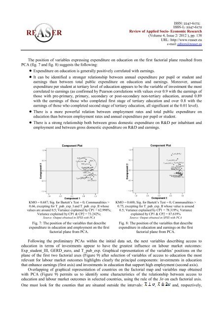
ISSN: 2247-6172;ISSN-L: 2247-6172Review of Applied Socio- Economic Research(Volume 4, Issue 2/ 2012 ), pp. 138URL: http://www.reaser.eue-mail: editors@reaser.euThe position of variables expressing expenditure on education on the first factorial plane resulted fromPCA (fig. 7 and fig. 8) suggests the following: Expenditure on education is generally positively correlated with earnings. It can be identified a stronger relationship between annual expenditure per pupil or student andearnings than between total public expenditure on education and earnings. Moreover, annualexpenditure per student at tertiary level of education appears to be the variable of investment the mostcorrelated to earnings (as confirmed by Pearson correlations with values over 0.9 with the earnings ofthose with pre-primary, primary, secondary or post-secondary non-tertiary education, around 0.89with the earnings of those who completed first stage of tertiary education and over 0.8 with theearnings of those who completed second stage of tertiary education, all significant at the 0.01 level). There is a more powerful relation between employment rates and total public expenditure oneducation than between employment rates and annual expenditure per pupil or student. There is a strong relationship both between gross domestic expenditure on R&D per inhabitant andemployment and between gross domestic expenditure on R&D and earnings.KMO = 0.687; Sig. for Bartett’s Test = 0; Communalities >0.66, excepting for T_pub_exp_I and T_pub_exp_II whosevalues are around 0.5; Variance explained by CP1 = 62.998%;Variance explained by CP1 & CP2 = 73.242%;Source: Output obtained in SPSS with PCAFig. 7: The position of the variables that describeexpenditure in education and employment on the firstfactorial plane from PCA.KMO = 0.688; Sig. for Bartett’s Test = 0; Communalities >0.75, excepting for T_pub_exp_II whose value is around0.5; Variance explained by CP1 = 78.319%; Varianceexplained by CP1 & CP2 = 87.619%Source: Output obtained in SPSS with PCAFig. 8: The position of the variables that describeexpenditure in education and earnings on the firstfactorial plane from PCA.Following the preliminary PCAs within the initial data set, the next variables describing access toeducation in terms of investments appear to have the greatest influence on labour market outcomes:Exp_student_III, GERD_euro, and T_pub_exp. Graphical representation of the variables’ positions on theplane of the first two factorial axes (Figure 9) after selection of variables of access to education the mostrelevant for labour market outcomes highlights clearly the principal components: investments in educationthat enhance earnings (first axis) and investments in education that support high employment (second axis).Overlapping of graphical representation of countries on the factorial map and variables map obtainedwith PCA (Figure 9) permits us to identify some characteristics of the relationship between access toeducation and labour market outcomes in selected countries, using the rule of the 3σ on each factorial axis.One must look for the counties that are situated outside the intervals: , and, respectively,