Effect of Maximum Probe Spacing of Soil Resistivity Survey on ...

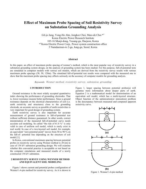
Apparent resistivity <strong>of</strong> probe spacing a can be calculated bythe equation (1). R is a measured apparent resistance .ρ a =2πaR (1)If the earth is uniform material with constant resistivity, theapparent resistivity should not be varied with varying probespacing. However, it is seldom the case in real world. Then,the apparent resistivity changes with varying probe spacing.Figure 2 shows an example <strong>of</strong> horizontally layered earthstrcucture (4 layer).Figure 2. Multi-layered soil modelTo obtain an soil model with simple structure (e.g.. ahorizontally layered model) equivalent to the measuredapparent resistivities, we describe the following optimizationproblem.mMinimize Σ |ρ a (i)-ρ c (i)| (2)i(ρ a (i) : i-th measured apparent resistivity,ρ c (i) : i-th calculated apparent resistivity,ρ c (i) = f(a i , ρ 1 , ρ 2 , ρ 3 ,…,ρ n , h 1 , h 2 , h 3 ,…h n-1 ),ρ n : resistivity <strong>of</strong> n-th layer earth,h n : thinkness <strong>of</strong> n-th layer earth,m : # <strong>of</strong> resistivity measurement)Figure 3 shows the site we conducted the survey <strong>of</strong>resistivities and fall-<strong>of</strong>-potential test.560 mFOP survey lineHorizontally layered soil model with 4 layers is assumed t<strong>of</strong>it the computed apparent resistivities to measured ones. <strong>Soil</strong>model parameters (i.e. layer resistivities and thinkness) arelisted in Table 1~3 with different maximum probe spacings.Figure 4 is the comparison results <strong>of</strong> computed and measuredresistivities.apparent resistivity [ohm-m]10000100010010measuredcalculated0.1 1 10 100 1000probe spacing [m]Figure 4. Measured and computed apparent resistivitiesTable 1~3 show an effect <strong>of</strong> maximum probe spacing onequivalent soil modeling that larger probe spacing produceshigher resistivity <strong>of</strong> bottom layer. In other words, it can be saidthat smaller probe spacing means relatively insufficientinformation on deeper earth. It should be noted the followingsoil models are equivalent to the apparent resistivity curvesshown in Figure 4, and not necessarily equivalent to the soilstructure physically.Table 1. <strong>Soil</strong> model #1 (Max.spacing:120m)<strong>Resistivity</strong> [Ωm] Thinkness [m]Top layer 131.8 2.0Central layer #1 284.2 4.2Central layer #2 176.5 12.8Bottom layer 3837.1 ∞Table 2. <strong>Soil</strong> model #2 (Max.spacing:50m)<strong>Resistivity</strong> [Ωm] Thinkness [m]Top layer 131.7 2.1Central layer #1 288.8 4.4Central layer #2 144.2 8.5Bottom layer 1725.0 ∞road<strong>Resistivity</strong> survey linesTable 3. <strong>Soil</strong> model #3 (Max.spacing:30m)<strong>Resistivity</strong> [Ωm] Thinkness [m]Top layer 132.6 2.4Central layer #1 398.0 2.3Central layer #2 168.5 11.3Bottom layer 1578.0 ∞Figure 3. Apparent resistivity and FOP survey lines

3 FALL-OF-POTENTIAL TEST ON A SUBSTATIONGROUNDING GRID WITH BORING ELECTRODESFigure 5 shows the configuration <strong>of</strong> 154 kV substationgrounding grid builded at the site shown in Figure 3. Inaddition to grounding grid, 6 deep-driven rods were installedto minimize ground resistance. The length <strong>of</strong> rods ranges up to33 meter and is limited by bedrocks under the site.15m70mdifference <strong>of</strong> computed & measured resistance35%30%25%20%15%10%5%model #1(120m)model #2(50m)model #3(30m)49m13m12m0%0 50 100 150 200 250 300 350 400 450 500potential probe distance [m]Figure 7. Differences between measured and computed values33m23mFigure 5. Configuration <strong>of</strong> the substation grounding gridAfter construction <strong>of</strong> the grounding grid and deep-drivenrods, fall-<strong>of</strong>-potential test were conducted to measure groundresistance <strong>of</strong> the grid. Simultaneously, three computer modelswere constructed to compare and verify the measured valueswith the computed ones. For the simulaton, multi-layeredversion <strong>of</strong> MALT program was used [6].Figure 6 shows the measured and calculated fall-<strong>of</strong>-potentialcurves. The %difference <strong>of</strong> computed fall-<strong>of</strong>-potential curvesfrom the measured one is shown in Figure 7. Each computermodel has a same grounding grid model shown in Figure 5 anddifferent soil models listed in Table 1~3 respectively.apparent resistance [ohm]876543210measuredmodel #1(120m)model #2(50m)model #3(30m)0 50 100 150 200 250 300 350 400 450 500potential probe distance [m]Figure 6. Comparison <strong>of</strong> measured and computer FOP curves14mIn Figure 7, the larger error near the grounding grid can beexplained by the locally changed soil structure resulted fromexcavations near the grid. Considering a non-uniform andcomplicated structures <strong>of</strong> real earth, it can be sait that thesimulated fall-<strong>of</strong>-potential curve is well agreed with themeasured curve.Table 4 is a summary <strong>of</strong> simulated fall-<strong>of</strong>-potential testsusing MALT program. It clearly shows that #1 computermodel, which uses the soil model <strong>of</strong> 120 meter <strong>of</strong> maximumprobe spacing results, is best fit to measured values.Table 4. Summary <strong>of</strong> computer simulationsModel #1 Model #2 Model #3Rg_calc. 4.4 [Ω] 3.6 [Ω] 3.4 [Ω]Required 380 [m] 348 [m] 326 mlocation (69 %) (62 %) (58 %)Rg_meas. 4.8 [Ω] 4.4 [Ω] 4.2 [Ω]%Error 8.3 [%] 17.7 [%] 18.0 [%]( Rg_calc. : calculated ground resistance,Rg_meas. : measured apparent resistance at the requiredlocation <strong>of</strong> each model,Required location:Zero potential point in computer models)4 CONCLUSIONIn this paper, we have studied the effect <strong>of</strong> maximum probespacing <strong>of</strong> Wenner method on the analysis <strong>of</strong> substationgrounding system. Fall-<strong>of</strong>-potential test on a 154 kVsubstation grounding system and a detailed quantitativeanalysis <strong>of</strong> fall-<strong>of</strong>-potential curve near the grid were conductedto show that an accurate resistivity survey as possible is veryimportant to minimize an error <strong>of</strong> computer models <strong>of</strong>substation grounding grids. Based on this study, it isrecommended that a maximum probe spacing larger than 20meter <strong>of</strong> conventional spacing in 154 kV substation groundingdesign is required for more accurate grounding design andanalysis.

REFERENCES[1] IEEE Std 81-1983, IEEE guide for measuring earthresistivity, ground impedance and earth surface potentials <strong>of</strong> aground system, pp.23, 1983[2] F. Dawalibi, "Earth resistivity measurement interpretationtechniques", IEEE Trans. on PAS, Vol. PAS-103, No. 2, pp.374-382, Feb. 1984[3] SES, RESAP Users' Manual, 2000[4] F.Dawalibi,N.Barbeito,"Measurement and computations <strong>of</strong>the performance <strong>of</strong> grounding systems buried in multilayersoils", IEEE Trans. on PD, Vol. 6, No. 4, pp. 1483-1490,October 1991[5] F.P.Dawalibi, J.Ma, R.Southey, "Behaviour <strong>of</strong> groundingsystems in multilayer soils: a parametric analysis", IEEETrans. on PD, Vol. 9, No. 1, pp. 334-342, January 1994[6] SES, MALT Users' Manual, 2000[7] G. Tagg, Earth Resistances, , 1964[8] IEEE Std 80-2000, IEEE guide for safety in AC substationgrounding , 2000