A Tutorial on Support Vector Machines for Pattern Recognition

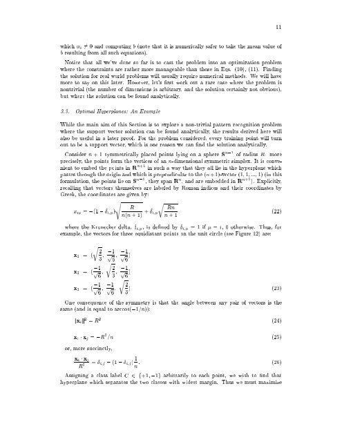
11which i 6= 0 and computing b (note that it is numerically safer to take the mean value ofb resulting from all such equations).Notice that all we've done so far is to cast the problem into an optimization problemwhere the constraints are rather more manageable than those in Eqs. (10), (11). Findingthe solution for real world problems will usually require numerical methods. We willhavemore to say onthis later. However, let's rst work out a rare case where the problem isnontrivial (the number of dimensions is arbitrary, and the solution certainly not obvious),but where the solution can be found analytically.3.3. Optimal Hyperplanes: An ExampleWhile the main aim of this Section is to explore a non-trivial pattern recognition problemwhere the support vector solution can be found analytically, theresults derived here willalso be useful in a later proof. For the problem considered, every training point will turnout to be a support vector, which is one reason we can nd the solution analytically.Consider n +1 symmetrically placed points lying on a sphere S n;1 of radius R: moreprecisely, the points form the vertices of an n-dimensional symmetric simplex. It is convenienttoembed the points in R n+1 in such away thattheyalllieinthehyperplane whichpasses through the origin and which is perpendicular to the (n+1)-vector (1 1 ::: 1) (in thisformulation, the points lie on S n;1 , they span R n , and are embedded in R n+1 ). Explicitly,recalling that vectors themselves are labeled by Roman indices and their coordinates byGreek, the coordinates are given by:s rRRnx i = ;(1 ; i )n(n +1) + i(22)n +1where the Kronecker delta, i , is dened by i = 1 if = i, 0 otherwise. Thus, forexample, the vectors for three equidistant points on the unit circle (see Figure 12) are:r2x 1 = (3 ;1p 6x 2 = ( ;1 p6x 3 = ( ;1 p6;1p6)r23 ;1p6);1p6r23 ) (23)One consequence of the symmetry is that the angle between any pair of vectors is thesame (and is equal to arccos(;1=n)):kx i k 2 = R 2 (24)x i x j = ;R 2 =n (25)or, more succinctly,x i x jR 2 = ij ; (1 ; ij ) 1 n : (26)Assigning a class label C 2 f+1 ;1g arbitrarily to each point, we wish to nd thathyperplane which separates the two classes with widest margin. Thus we must maximize