A Tutorial on Support Vector Machines for Pattern Recognition

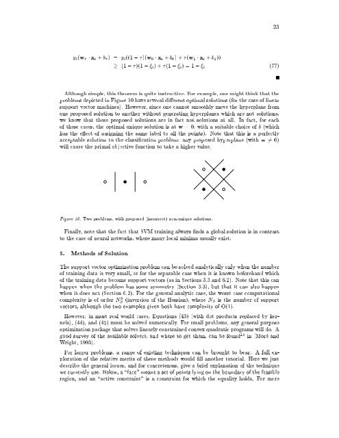
23y i (w x i + b ) = y i ((1 ; )(w 0 x i + b 0 )+(w 1 x i + b 1 )) (1 ; )(1 ; i )+(1 ; i )=1; i (77)Although simple, this theorem is quite instructive. For example, one might think that theproblems depicted in Figure 10 have several dierent optimal solutions (for the case of linearsupport vector machines). However, since one cannot smoothly move thehyperplane fromone proposed solution to another without generating hyperplanes which are not solutions,we know that these proposed solutions are in fact not solutions at all. In fact, for eachof these cases, the optimal unique solution is at w = 0, with a suitable choice of b (whichhas the eect of assigning the same label to all the points). Note that this is a perfectlyacceptable solution to the classication problem: any proposed hyperplane (with w 6= 0)will cause the primal objective function to take a higher value.Figure 10. Two problems, with proposed (incorrect) non-unique solutions.Finally, note that the fact that SVM training always nds a global solution is in contrastto the case of neural networks, where many local minima usually exist.5. Methods of SolutionThe support vector optimization problem can be solved analytically only when the numberof training data is very small, or for the separable case when it is known beforehand whichof the training data become support vectors (as in Sections 3.3 and 6.2). Note that this canhappen when the problem has some symmetry (Section 3.3), but that it can also happenwhen it does not (Section 6.2). For the general analytic case, the worst case computationalcomplexity is of order N 3 S (inversion of the Hessian), where N S is the number of supportvectors, although the two examples given both have complexity of O(1).However, in most real world cases, Equations (43) (with dot products replaced by kernels),(44), and (45) must be solved numerically. For small problems, any general purposeoptimization package that solves linearly constrained convex quadratic programs will do. Agood survey of the available solvers, and where to get them, can be found 16 in (More andWright, 1993).For larger problems, a range of existing techniques can be brought to bear. A full explorationof the relative merits of these methods would ll another tutorial. Here we justdescribe the general issues, and for concreteness, give a brief explanation of the techniquewe currently use. Below, a \face" means a set of points lying on the boundary of the feasibleregion, and an \active constraint" is a constraint forwhich theequality holds. For more