Decomposition of the elastic tensor and geophysical applications
Decomposition of the elastic tensor and geophysical applications
Decomposition of the elastic tensor and geophysical applications

Create successful ePaper yourself
Turn your PDF publications into a flip-book with our unique Google optimized e-Paper software.
Geophys. J. Int. (2004) 159, 667–678doi: 10.1111/j.1365-246X.2004.02415.x<strong>Decomposition</strong> <strong>of</strong> <strong>the</strong> <strong>elastic</strong> <strong>tensor</strong> <strong>and</strong> <strong>geophysical</strong> <strong>applications</strong>Jules Thomas Browaeys 1 <strong>and</strong> Sébastien Chevrot 21 Laboratoire de Dynamique des Systèmes Géologiques, CNRS, UMR 7579, Institut de Physique du Globe, Paris, France. E-mail: browaeys@ipgp.jussieu.fr2 Laboratoire de Dynamique Terrestre et Planétaire, CNRS, UMR 5562, Observatoire Midi-Pyrénées, Toulouse, France. E-mail: Sebastien.Chevrot@cnes.frAccepted 2004 June 14. Received 2004 June 14; in original form 2003 November 10SUMMARYElasticity is described in general by a fourth-order <strong>tensor</strong> with 21 independent coefficients,which corresponds to <strong>the</strong> triclinic symmetry class. However seismological observations areusually explained with a higher order <strong>of</strong> symmetry using fewer parameters. We propose ananalytical method to decompose <strong>the</strong> <strong>elastic</strong> <strong>tensor</strong> into a sum <strong>of</strong> orthogonal <strong>tensor</strong>s belonging to<strong>the</strong> different symmetry classes. The method relies on a vectorial description <strong>of</strong> <strong>the</strong> <strong>elastic</strong> <strong>tensor</strong>.Any symmetry class constitutes a subspace <strong>of</strong> a class <strong>of</strong> lower symmetry <strong>and</strong> an orthogonalprojection on this subspace removes <strong>the</strong> lower symmetry part. Orthogonal projectors on eachhigher symmetry class are given explicitly. In addition, <strong>the</strong> method provides optimal highersymmetry approximations, which allow us to decrease <strong>the</strong> number <strong>of</strong> independent parameters.Consequences <strong>of</strong> <strong>the</strong> symmetry approximation <strong>of</strong> <strong>the</strong> <strong>elastic</strong> <strong>tensor</strong> on shear wave splitting(SWS) are investigated for upper-mantle minerals (olivine <strong>and</strong> enstatite), natural samples <strong>and</strong>numerically deformed olivine aggregates. The orthorhombic part <strong>of</strong> <strong>the</strong> <strong>elastic</strong> <strong>tensor</strong> as wellas <strong>the</strong> presence <strong>of</strong> enstatite are important second-order effects.Key words: <strong>elastic</strong> <strong>tensor</strong>, seismic anisotropy, symmetry class, upper mantle.1 INTRODUCTIONSeismic anisotropy in <strong>the</strong> upper mantle <strong>of</strong> <strong>the</strong> Earth results mainly from lattice preferred orientation (LPO) <strong>of</strong> its main constitutive minerals,olivine <strong>and</strong> orthopyroxene, which are strongly anisotropic (Nicolas & Christensen 1987). Because LPO is produced by deformation <strong>of</strong> rocks,observations <strong>of</strong> seismic anisotropy can be used to constrain <strong>the</strong> pattern <strong>of</strong> convective flow in <strong>the</strong> mantle (Ribe 1992; Zhang & Karato 1995).Different seismic waves are used to study mantle anisotropy. Inversions <strong>of</strong> surface wave data yield 3-D images <strong>of</strong> anisotropy with typicallateral <strong>and</strong> vertical resolutions <strong>of</strong> 1000 <strong>and</strong> 100 km, respectively (Montagner & Nataf 1986, 1988; Montagner & Tanimoto 1991; Trampert &Woodhouse 1995). In contrast, shear wave splitting (SWS) measurements provide precise estimates <strong>of</strong> <strong>the</strong> polarization direction <strong>of</strong> <strong>the</strong> fastS wave <strong>and</strong> S delay time beneath receivers, but have poor depth resolution (Silver & Chan 1991; Favier & Chevrot 2003). These differentapproaches share a need for restrictive simplifying assumptions about <strong>the</strong> symmetry <strong>of</strong> <strong>the</strong> anisotropic medium to ensure tractability. In <strong>the</strong>case <strong>of</strong> surface waves, an artificial distinction is made between azimuthal anisotropy (Smith & Dahlen 1973) that uses a horizontal hexagonalaxis <strong>and</strong> radial anisotropy that assumes hexagonal symmetry with a vertical axis (an <strong>elastic</strong> medium with hexagonal symmetry is equivalentto a transversely isotropic medium). Studies <strong>of</strong> SWS generally use a small number <strong>of</strong> uniform hexagonal layers with a horizontal symmetryaxis. While such assumptions may be reasonable far from plate boundaries, <strong>the</strong>y are probably invalid in regions such as ridges, hotspots <strong>and</strong>subduction zones where mantle flow is likely to generate complex variations <strong>of</strong> anisotropy over short length scales (Kaminski & Ribe 2002).A promising approach is forward modelling <strong>of</strong> anisotropy produced by mantle flow using polycrystalline plasticity models (Wenk &Tomé 1999; Kaminski & Ribe 2001). Such calculations yield <strong>the</strong> anisotropic <strong>elastic</strong> <strong>tensor</strong> at all points in <strong>the</strong> domain under study, fromwhich syn<strong>the</strong>tic seismograms may be calculated <strong>and</strong> compared with observations (Blackman et al. 2002a; Blackman & Kendall 2002b). Thisapproach requires no ad hoc assumptions about <strong>the</strong> relation between LPO <strong>and</strong> flow <strong>and</strong>, in principle, <strong>the</strong> comparison between predictions <strong>and</strong>observations should help discriminate between c<strong>and</strong>idate geodynamic models. The determination <strong>of</strong> <strong>the</strong> symmetry <strong>of</strong> <strong>the</strong> predicted <strong>elastic</strong><strong>tensor</strong> can help in evaluating whe<strong>the</strong>r simplified <strong>elastic</strong> models assumed in inverse problems (e.g., a hexagonal medium with a horizontalsymmetry axis) are appropriate representations <strong>of</strong> <strong>the</strong> more complicated geodynamic structures. An analysis <strong>of</strong> <strong>the</strong> symmetry <strong>of</strong> <strong>elastic</strong><strong>tensor</strong>s calculated from LPO observed in natural samples (Mainprice & Silver 1993) allows also to compare <strong>the</strong> latter more effectively withnumerically predicted <strong>elastic</strong> <strong>tensor</strong>s. Because seismologists are used to describing seismic anisotropy in terms <strong>of</strong> orientation <strong>of</strong> <strong>the</strong> symmetryaxis <strong>and</strong> amplitude <strong>of</strong> anisotropy, it is useful to make use <strong>of</strong> a method to find a representation <strong>of</strong> any <strong>elastic</strong> <strong>tensor</strong> in terms <strong>of</strong> an optimalhexagonal <strong>elastic</strong> medium. More generally, we will show that any <strong>elastic</strong> <strong>tensor</strong> can be decomposed into contributions corresponding todifferent symmetry classes.GJI SeismologyC○ 2004 RAS 667
668 J. T. Browaeys <strong>and</strong> S. ChevrotWe introduce an analytical method for <strong>the</strong> symmetry decomposition <strong>of</strong> <strong>elastic</strong> <strong>tensor</strong>s based upon orthogonal projections on subspaces.The representation <strong>of</strong> <strong>the</strong> fourth-order <strong>elastic</strong> <strong>tensor</strong> by a second-order <strong>tensor</strong>, preserving its ma<strong>the</strong>matical properties, was first proposed byKelvin (1856). Unfortunately, this convenient ma<strong>the</strong>matical description is less popular than <strong>the</strong> widespread Voigt representation (Helbig 1994).Symmetry <strong>of</strong> <strong>the</strong> <strong>elastic</strong> <strong>tensor</strong> becomes visible when it is expressed in its natural coordinate system whose axes correspond to directions <strong>of</strong>symmetry. In a pioneering study, Cowin & Mehrabadi (1987) proposed a method for finding <strong>the</strong> normals to <strong>the</strong> symmetry planes <strong>of</strong> <strong>the</strong> <strong>elastic</strong><strong>tensor</strong>. Arts et al. (1991) introduced an analytical method to find <strong>the</strong> optimal approximation <strong>of</strong> a given symmetry class for any <strong>elastic</strong> <strong>tensor</strong>.They use <strong>the</strong> coordinate system obtained by <strong>the</strong> method <strong>of</strong> Cowin & Mehrabadi (1987) <strong>and</strong> minimize <strong>the</strong> distance between <strong>the</strong> <strong>tensor</strong> <strong>and</strong>its representation in a given symmetry class. This gives a system <strong>of</strong> linear equations for <strong>the</strong> approximate <strong>elastic</strong> coefficients. This method iseffective for media close to orthorhombic or <strong>of</strong> higher symmetry. Helbig (1995) proposed <strong>the</strong> representation <strong>of</strong> fourth-order <strong>elastic</strong> <strong>tensor</strong>sby vectors in a 21-dimensional vector space. Using this representation, approximations <strong>of</strong> <strong>the</strong> <strong>elastic</strong> <strong>tensor</strong> can be seen as projections onto asubspace describing a higher symmetry <strong>tensor</strong>.In this article, we extend <strong>the</strong> approach <strong>of</strong> Arts et al. (1991); Arts (1993) <strong>and</strong> Helbig (1995) in order to present a practical method thatrealizes <strong>the</strong>se approximations. We first describe <strong>the</strong> vectorial representation <strong>of</strong> <strong>elastic</strong> <strong>tensor</strong>s <strong>and</strong> <strong>the</strong> projections that allow to pass from agiven symmetry to any higher order symmetry class. An exact <strong>and</strong> practical version <strong>of</strong> <strong>the</strong> <strong>elastic</strong> <strong>tensor</strong> approximation method is formulated.Finally, we consider various <strong>applications</strong> <strong>of</strong> <strong>the</strong> decomposition method to <strong>geophysical</strong> problems <strong>and</strong> investigate <strong>the</strong> consequences <strong>of</strong> symmetryapproximations using materials representative <strong>of</strong> <strong>the</strong> upper mantle.2 FROM THE ELASTIC TENSOR TO THE ELASTIC VECTORElastic properties are ma<strong>the</strong>matically described by Hooke’s law, which relates deformation to stress through a fourth-order <strong>elastic</strong> <strong>tensor</strong>described by 81 coefficients. The symmetry <strong>of</strong> <strong>the</strong> stress <strong>tensor</strong> σ ij <strong>and</strong> <strong>the</strong> strain <strong>tensor</strong> ε ij reduces <strong>the</strong> number <strong>of</strong> independent <strong>elastic</strong>coefficients from 81 to 36 <strong>and</strong> <strong>the</strong> requirement that <strong>the</strong> <strong>elastic</strong> energy be completely defined by <strong>the</strong> strain <strong>tensor</strong> or <strong>the</strong> stress <strong>tensor</strong> fur<strong>the</strong>rdecreases this number to 21 for a triclinic medium. Media with higher symmetry require fewer parameters for <strong>the</strong>ir description. A convenientrepresentation <strong>of</strong> <strong>the</strong> <strong>elastic</strong> coefficients is <strong>the</strong> so-called Voigt notation. The Voigt matrix is a six-dimensional symmetric array C IJ whoseelements are related to <strong>the</strong> c ijkl according to <strong>the</strong> rules:C IJ = c ijklwith{I = iδij + (1 − δ ij )(9 − i − j)J = kδ kl + (1 − δ kl )(9 − k − l).(2.1)The Voigt matrix is however not a <strong>tensor</strong> <strong>and</strong> no longer preserves <strong>the</strong> ma<strong>the</strong>matical properties <strong>of</strong> c ijkl .For <strong>elastic</strong>ity, <strong>the</strong>re are eight distinctsymmetry classes: triclinic, monoclinic, orthorhombic, tetragonal, trigonal, hexagonal, cubic <strong>and</strong> isotropic. A higher symmetry class canbe seen as a special case <strong>of</strong> a lower symmetry class, defined by additional relationships between coefficients (Helbig 1995). Increasing <strong>the</strong>symmetry <strong>of</strong> a medium by adding symmetry planes decreases <strong>the</strong> number <strong>of</strong> independent parameters.A useful representation <strong>of</strong> <strong>elastic</strong> <strong>tensor</strong>s is in terms <strong>of</strong> vectors in a 21-dimensional vectorial space. The basis vectors correspond to 21elementary <strong>tensor</strong>s c (1) , ..., c (21) as shown in Table 1. Any <strong>elastic</strong> <strong>tensor</strong> can be represented as an <strong>elastic</strong> vector X whose components are:t X =(C 11 ,C 22 ,C 33 , √ 2C 23 , √ 2C 13 , √ 2C 12 ,2C 44 ,2C 55 ,2C 66 ,2C 14 ,2C 25 ,2C 36 ,2C 34 ,2C 15 ,2C 26 ,2C 24 ,2C 35 ,2C 16 ,2 √ 2C 56 ,2 √ 2C 46 ,2 √ )2C 45= (X 1 , X 2 , X 3 , X 4 , X 5 , X 6 , X 7 , X 8 , X 9 , X 10 , X 11 , X 12 , X 13 , X 14 , X 15 , X 16 , X 17 , X 18 , X 19 , X 20 , X 21 ) . (2.2)The normalization factors that appear in <strong>the</strong> above expression reflect <strong>the</strong> multiplicity <strong>of</strong> <strong>the</strong> <strong>elastic</strong> <strong>tensor</strong> components <strong>and</strong> are included so that<strong>the</strong> Euclidean norm <strong>of</strong> an arbitrary <strong>elastic</strong> <strong>tensor</strong> c <strong>and</strong> its associated <strong>elastic</strong> vector X are identical. These norms are defined byN(c) = √ 〈c, c〉 = √ 〈X, X〉 =N(X), (2.3)where <strong>the</strong> scalar product <strong>of</strong> arbitrary <strong>tensor</strong>s c (1) <strong>and</strong> c (2) or <strong>the</strong>ir associated vectors X (1) <strong>and</strong> X (2) is〈c (1) , c (2)〉 = c (1)ijkl c(2) ijkl = X (1)i X (2)i = 〈 X (1) , X (2)〉 . (2.4)3 DECOMPOSITION OF THE ELASTIC TENSOR BY PROJECTION3.1 Principle <strong>of</strong> <strong>the</strong> orthogonal projection methodA projector in <strong>the</strong> 21-D <strong>elastic</strong> vectorial space is described by a 21 × 21 matrix. Let us consider <strong>the</strong> <strong>elastic</strong> vector X that belongs to a subspaceS <strong>of</strong> dimension N S <strong>of</strong> <strong>the</strong> 21-D vectorial space. A higher symmetry class corresponds to a subspace H <strong>of</strong> S. Therefore, <strong>the</strong> <strong>elastic</strong> vector Xcan be decomposed asX = X H + X D , (3.1)C○ 2004 RAS, GJI, 159, 667–678
<strong>Decomposition</strong> <strong>of</strong> <strong>the</strong> <strong>elastic</strong> <strong>tensor</strong> <strong>and</strong> <strong>geophysical</strong> <strong>applications</strong> 669Table 1. Definition <strong>of</strong> <strong>the</strong> elementary <strong>tensor</strong>s c (1) , ..., c (21) associated to <strong>the</strong> 21 orthonormalbasis vectors. Voigt matrix elements are also shown.Fourth- Non-zero Non-zeroorder c ijkl C IJ<strong>tensor</strong> elements elementsc (1) c 1111 = 1 C 11 = 1c (2) c 2222 = 1 C 22 = 1c (3) c 3333 = 1 C 33 = 1c (4) c 2233 = c 3322 = 1/ √ 2 C 23 = C 32 = 1/ √ 2c (5) c 1133 = c 3311 = 1/ √ 2 C 13 = C 31 = 1/ √ 2c (6) c 1122 = c 2211 = 1/ √ 2 C 12 = C 21 = 1/ √ 2c (7) c 2323 = c 2332 = c 3223 = c 3232 = 1/2 C 44 = 1/2c (8) c 1313 = c 1331 = c 3113 = c 3131 = 1/2 C 55 = 1/2c (9) c 1212 = c 2332 = c 2112 = c 2121 = 1/2 C 66 = 1/2c (10) c 1123 = c 1132 = c 2311 = c 3211 = 1/2 C 14 = C 41 = 1/2c (11) c 2213 = c 2231 = c 1322 = c 3122 = 1/2 C 25 = C 52 = 1/2c (12) c 3312 = c 3321 = c 1233 = c 2133 = 1/2 C 36 = C 63 = 1/2c (13) c 3323 = c 3332 = c 2333 = c 3233 = 1/2 C 34 = C 43 = 1/2c (14) c 1113 = c 1131 = c 1311 = c 3111 = 1/2 C 15 = C 51 = 1/2c (15) c 2212 = c 2221 = c 1222 = c 2122 = 1/2 C 26 = C 62 = 1/2c (16) c 2223 = c 2232 = c 2322 = c 3222 = 1/2 C 24 = C 42 = 1/2c (17) c 3313 = c 3331 = c 1333 = c 3133 = 1/2 C 35 = C 53 = 1/2c (18) c 1112 = c 1121 = c 1211 = c 2111 = 1/2 C 16 = C 61 = 1/2c (19) c 1312 = c 1321 = c 3112 = c 3121 = c 1213= c 1231 = c 2113 = c 2131 = (2 √ 2) −1C 56 = C 65 = (2 √ 2) −1c (20) c 2312 = c 2321 = c 3212 = c 3221 = c 1223 C 46 = C 64 = (2 √ 2) −1= c 1232 = c 2123 = c 2132 = (2 √ 2) −1c (21) c 2313 = c 2331 = c 3213 = c 3231 = c 1323 C 45 = C 54 = (2 √ 2) −1= c 1332 = c 3123 = c 3132 = (2 √ 2) −1where X H belongs to H <strong>and</strong> <strong>the</strong> deviation vector X D to <strong>the</strong> subspace orthogonal to H (Helbig 1995). Let p denote an orthogonal projector fromsubspace S onto subspace H. If(S 1 , ..., S NS )isanorthonormal basis <strong>of</strong> <strong>the</strong> subspace S with (S 1 , ..., S NH ) belonging to H <strong>and</strong> (S NH +1, ...,S NS )to<strong>the</strong> subspace orthogonal to H, <strong>the</strong> deviation vector X D constituting <strong>the</strong> lower symmetry part <strong>of</strong> <strong>the</strong> vector is given byX D = ( X · S NH +1)SNH +1 + ···+ ( )X · S NS SNS (3.2)<strong>and</strong> <strong>the</strong> projector on subspace H is defined byp(X) = I (X) − (X · X D )X D = X H , (3.3)where I is <strong>the</strong> identity operator. The specific relationships satisfied by <strong>the</strong> coefficients <strong>of</strong> a vector that lies in <strong>the</strong> subspace H allow one t<strong>of</strong>ind <strong>the</strong> set <strong>of</strong> vectors (S NH +1, ..., S NS ) that are orthogonal to H. This set is completed by (S 1 , ..., S NH ) belonging to H in order to give anappropriate orthonormal basis <strong>of</strong> S for <strong>the</strong> projection on H.We explain in Appendix A how to calculate elementary projectors corresponding to a projection from a symmetry class to <strong>the</strong> next higherorder symmetry class. We <strong>the</strong>n give matrix expressions <strong>of</strong> more general projectors from any symmetry class onto a higher symmetry class bycomposing elementary projectors.3.2 Symmetry cartesian coordinate systemThe norm <strong>and</strong> scalar product defined by eqs (2.3) <strong>and</strong> (2.4) are invariant under rotation <strong>of</strong> <strong>the</strong> 3-D cartesian coordinate system. However,<strong>the</strong> coefficients <strong>of</strong> <strong>the</strong> 21-D vector X depend both on <strong>the</strong> 3-D cartesian coordinate system <strong>and</strong> on <strong>the</strong> decomposition method. Finding <strong>the</strong>appropriate 3-D cartesian coordinate system for <strong>the</strong> projection method requires one to determine <strong>the</strong> orientations <strong>of</strong> <strong>the</strong> symmetry elements.Cowin & Mehrabadi (1987) define necessary <strong>and</strong> sufficient conditions for a vector to be normal to a symmetry plane. In particular, <strong>the</strong>ydemonstrate that such a vector must be an eigenvector <strong>of</strong> both <strong>the</strong> dilatational stiffness <strong>tensor</strong> d ij = c ijkk <strong>and</strong> <strong>the</strong> Voigt stiffness <strong>tensor</strong> v ik =c ijkj ,which are given by⎡⎤C 11 + C 12 + C 13 C 16 + C 26 + C 36 C 15 + C 25 + C 35⎢⎥d = ⎣C 16 + C 26 + C 36 C 12 + C 22 + C 32 C 14 + C 24 + C 34 ⎦ , (3.4)C 15 + C 25 + C 35 C 14 + C 24 + C 34 C 13 + C 23 + c 33C○ 2004 RAS, GJI, 159, 667–678
670 J. T. Browaeys <strong>and</strong> S. ChevrotTable 2. Structure <strong>of</strong> <strong>the</strong> eigenspaces <strong>of</strong> d ij <strong>and</strong> v ik <strong>and</strong> <strong>the</strong> relation with <strong>the</strong>symmetry cartesian coordinate system (SCCS) for <strong>the</strong> different symmetryclasses.Elastic Distinct Coincident Symmetrysymmetry eigenvalues eigenvectors cartesianclass <strong>of</strong> d ij & v ik <strong>of</strong> d ij & v ik coordinate axesTriclinic 3 0 No particularityMonoclinic 3 1 Three-axis is <strong>the</strong> singlecommon eigenvectorOrthorhombic 3 3 Axes are <strong>the</strong> threecommon eigenvectorsTetragonal 2 3 Three-axis is <strong>the</strong> nondegenerateeigenvectorHexagonal 2 3 Three-axis is <strong>the</strong> nondegenerateeigenvectorIsotropic 1 3 No particularity⎡⎤C 11 + C 66 + C 55 C 16 + C 26 + C 45 C 15 + C 35 + C 46⎢⎥v = ⎣C 16 + C 26 + C 45 C 66 + C 22 + C 44 C 24 + C 34 + C 56 ⎦ . (3.5)C 15 + C 35 + C 46 C 24 + C 34 + C 56 C 55 + C 44 + C 33While a general fourth-order <strong>tensor</strong> has six distinct contractions <strong>of</strong> rank two, <strong>the</strong> symmetries <strong>of</strong> <strong>elastic</strong> <strong>tensor</strong>s reduce <strong>the</strong> number <strong>of</strong> distinctcontractions to two, which are conventionally chosen to be d ij <strong>and</strong> v ik (Helbig 1994). Physically, <strong>the</strong> principal directions <strong>of</strong> d ij are <strong>the</strong> principaldirections <strong>of</strong> <strong>the</strong> stress <strong>tensor</strong> σ (d)ij required to produce an isotropic dilatation ε ij = ɛδ ij <strong>of</strong> <strong>the</strong> anisotropic medium:σ (d)ij = c ijkl ε kl = c ijkl ɛδ kl = ɛd ij . (3.6)The three principal directions <strong>of</strong> v ik are <strong>the</strong> three phase propagation directions corresponding to extreme <strong>of</strong> <strong>the</strong> quantityQ = ρ ( V 2 P + V 2 S1 + V S2) 2 , (3.7)where ρ is <strong>the</strong> density <strong>and</strong> V P , V S1 <strong>and</strong> V S2 are <strong>the</strong> phase velocities <strong>of</strong> P wave, fast S wave <strong>and</strong> slow S wave, respectively. Table 2 describes<strong>the</strong> structure <strong>of</strong> <strong>the</strong> eigenspaces <strong>of</strong> d ij <strong>and</strong> v ik <strong>and</strong> <strong>the</strong> relation between <strong>the</strong> symmetry cartesian coordinate system (SCCS) <strong>and</strong> <strong>the</strong> eigenvectorsfor <strong>the</strong> different symmetry classes. For media with orthorhombic or higher symmetry, <strong>the</strong> eigenvectors <strong>of</strong> d ij <strong>and</strong> v ik are identical <strong>and</strong> defineuniquely <strong>the</strong> SCCS (Bennett 1972; Helbig 1994). For an orthorhombic medium, <strong>the</strong> three eigenvectors are normal to <strong>the</strong> three perpendicularsymmetry planes. For tetragonal <strong>and</strong> hexagonal media, only two <strong>of</strong> <strong>the</strong> eigenvalues are distinct. Accordingly, <strong>the</strong> only well-defined axis is<strong>the</strong> one along <strong>the</strong> non-degenerate eigenvector, which corresponds to <strong>the</strong> 2π/4 symmetry axis (tetragonal) or <strong>the</strong> transverse isotropy axis(hexagonal). The choice <strong>of</strong> <strong>the</strong> o<strong>the</strong>r two axes is arbitrary. All three axes are arbitrary for an isotropic medium, for which any vector is aneigenvector <strong>of</strong> both d ij <strong>and</strong> v ik .Amonoclinic medium has a single eigenvector common to d ij <strong>and</strong> v ik ,which is normal to <strong>the</strong> unique symmetryplane. Finally, a triclinic medium has no eigenvalues common to d ij <strong>and</strong> v ik , <strong>and</strong> <strong>the</strong> choice <strong>of</strong> <strong>the</strong> SCCS is arbitrary. For a symmetry lowerthan orthorhombic, <strong>the</strong> three SCCS directions are chosen as <strong>the</strong> bisectrix <strong>of</strong> each pair <strong>of</strong> one d ij eigenvector <strong>and</strong> <strong>the</strong> corresponding closest v ikeigenvector. This choice is appropriate <strong>and</strong> stable for a small triclinic part (less than 2–3 per cent) (Arts 1993).3.3 <strong>Decomposition</strong> <strong>of</strong> <strong>the</strong> <strong>elastic</strong> <strong>tensor</strong>Any triclinic vector X in a given 3-D cartesian coordinate system can be decomposed by a cascade <strong>of</strong> projections into a sum <strong>of</strong> vectorsbelonging to <strong>the</strong> different symmetry classes:X = X tric + X mon + X ort + X tet + X hex + X iso . (3.8)The space <strong>of</strong> <strong>elastic</strong> vectors has a finite dimension <strong>and</strong> thus all correctly defined norms are ma<strong>the</strong>matically equivalent, i.e. using a different normfrom eq. (2.3) will change distances but not <strong>the</strong> resulting decomposition. Moreover, as noted above, an important property <strong>of</strong> an orthogonalprojection is that <strong>the</strong> distance between a vector X <strong>and</strong> its orthogonal projection X H = p(X) onagiven subspace is minimum. These tw<strong>of</strong>eatures ensure that <strong>the</strong> decomposition is optimal once <strong>the</strong> 3-D Cartesian coordinate system is chosen.4 GEOPHYSICAL APPLICATIONSIn this section, we present <strong>the</strong> symmetry decomposition <strong>of</strong> <strong>elastic</strong> <strong>tensor</strong>s for three classes <strong>of</strong> media representative (supposedly) <strong>of</strong> <strong>the</strong> uppermantle: single crystals <strong>of</strong> olivine <strong>and</strong> enstatite, natural peridotite samples from <strong>the</strong> Kaapvaal craton in Africa, <strong>and</strong> olivine <strong>and</strong> enstatiteaggregates deformed numerically in a polycrystalline plasticity code. We also investigate <strong>the</strong> relation between SWS, finite strain <strong>and</strong> <strong>the</strong>hexagonal symmetry assumption. The SCCS directions indexes are chosen such that <strong>the</strong> 3-axis is always <strong>the</strong> hexagonal axis.C○ 2004 RAS, GJI, 159, 667–678
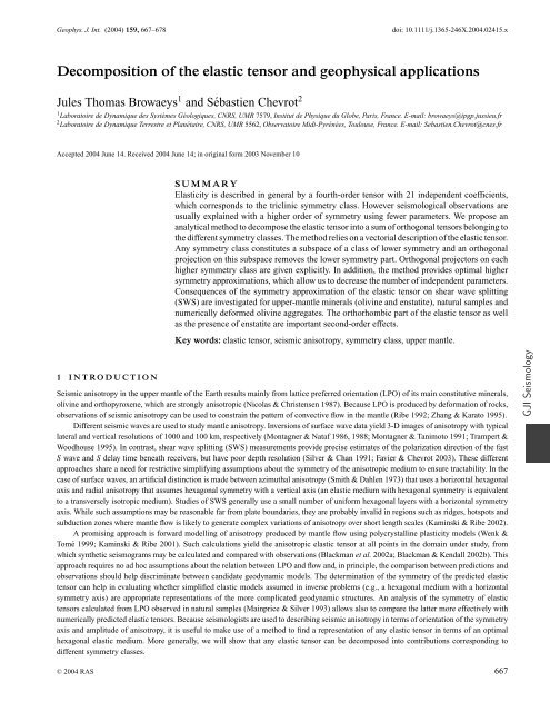
4.1 <strong>Decomposition</strong> <strong>of</strong> olivine <strong>and</strong> enstatite <strong>elastic</strong> <strong>tensor</strong>s<strong>Decomposition</strong> <strong>of</strong> <strong>the</strong> <strong>elastic</strong> <strong>tensor</strong> <strong>and</strong> <strong>geophysical</strong> <strong>applications</strong> 671According to mineralogical models <strong>of</strong> <strong>the</strong> upper mantle, olivine is <strong>the</strong> most abundant (∼70 per cent) <strong>and</strong> most deformable mineral, whileorthopyroxene is <strong>the</strong> secondary major mineral (∼30 per cent; Anderson 1989). Elastic coefficients are taken from Anderson & Isaak (1995)for olivine Fo 90 Fa 10 at 1500 K <strong>and</strong> from Bass (1995) for enstatite MgSiO 3 at room pressure <strong>and</strong> temperature.4.1.1 OlivineThe decomposition <strong>of</strong> <strong>the</strong> olivine <strong>elastic</strong> <strong>tensor</strong> in <strong>the</strong> different symmetry components is presented below in Voigt notation with <strong>elastic</strong>coefficients in GPa:⎛⎞ ⎛⎞192 66 60 0 0 0 16 0 2 0 0 066 160 56 0 0 00 −16 −2 0 0 060 56 272 0 0 0C IJ =⎜ 0 0 0 60 0 0⎟⎝⎠ = 2 −2 0 0 0 0⎜ 0 0 0 −1 0 0⎟⎝⎠+⎜⎝0 0 0 0 62 00 0 0 0 0 49⎛3 −3 0 0 0 0−3 3 0 0 0 00 0 0 0 0 00 0 0 0 0 00 0 0 0 0 00 0 0 0 0 −3⎞ ⎛⎟ +⎜⎠ ⎝T0 0 0 0 1 00 0 0 0 0 0−21.7 1.7 −9.3 0 0 01.7 −21.7 −9.3 0 0 0−9.3 −9.3 77.3 0 0 00 0 0 −2.7 0 00 0 0 0 −2.7 00 0 0 0 0 −11.7O⎞⎟⎠H⎛+⎜⎝194.7 67.3 67.3 0 0 067.3 194.7 67.3 0 0 067.3 67.3 194.7 0 0 00 0 0 63.7 0 00 0 0 0 63.7 00 0 0 0 0 63.7Subscripts are O for orthorhombic, T for tetragonal, H for hexagonal <strong>and</strong> I for isotropic. The isotropic approximation <strong>of</strong> olivine single crystalaccounts for 79.3 per cent <strong>of</strong> <strong>the</strong> norm <strong>of</strong> <strong>the</strong> <strong>tensor</strong> with isotropic moduli equal to K = 109.8 GPa <strong>and</strong> G = 63.7 GPa. The remaining anisotropicpart represents 20.7 per cent <strong>of</strong> <strong>the</strong> norm <strong>of</strong> <strong>the</strong> <strong>tensor</strong>. The different <strong>elastic</strong> symmetry parts <strong>of</strong> <strong>the</strong> <strong>tensor</strong> are presented as percentages <strong>of</strong> <strong>the</strong>norm <strong>of</strong> <strong>the</strong> <strong>elastic</strong> <strong>tensor</strong> in <strong>the</strong> histogram <strong>of</strong> Fig. 1 using <strong>the</strong> following convention:100 per cent = N −2 (X) [ N 2 (X tric ) + N 2 (X mon ) + N 2 (X ort ) + N 2 (X tet ) + N 2 (X hex ) + N 2 (X iso ) ] . (4.1)Anisotropic parts <strong>of</strong> <strong>the</strong> <strong>tensor</strong>s are mainly hexagonal <strong>and</strong> orthorhombic. Most <strong>of</strong> <strong>the</strong> anisotropy is hexagonal (15.2 per cent), while <strong>the</strong>remaining 5.5 per cent is tetragonal <strong>and</strong> orthorhombic (first column <strong>of</strong> Fig. 1).⎞.⎟⎠I4.1.2 EnstatiteEnstatite is less anisotropic (9.2 per cent) than olivine as <strong>the</strong> isotropic part accounts for 90.8 per cent <strong>of</strong> <strong>the</strong> norm <strong>of</strong> <strong>the</strong> <strong>elastic</strong> <strong>tensor</strong> (moduliare K = 108.3 GPa <strong>and</strong> G = 76.4 GPa). Anisotropy is distributed between <strong>the</strong> hexagonal part (4.3 per cent) <strong>and</strong> <strong>the</strong> tetragonal/orthorhombicpart (4.9 per cent). Addition <strong>of</strong> enstatite to <strong>the</strong> olivine decreases <strong>the</strong> total anisotropy as well as <strong>the</strong> orthorhombic part.⎛C IJ =⎜⎝225 54 72 0 0 054 214 53 0 0 072 53 178 0 0 00 0 0 78 0 00 0 0 0 82 00 0 0 0 0 76⎛+⎜⎝3.4 −3.4 0 0 0 0−3.4 3.4 0 0 0 00 0 0 0 0 00 0 0 0 0 00 0 0 0 0 00 0 0 0 0 −3.4⎞ ⎛⎟⎠ = ⎜⎝⎞ ⎛⎟ +⎜⎠ ⎝T55 0 95 0 0 00 −55 −95 0 0 095 −95 0 0 0 00 0 0 −2 0 00 0 0 0 2 00 0 0 0 0 0⎞⎟⎠5.9 1.7 5.1 0 0 00 5.9 5.1 0 0 05.1 5.1 −32.2 0 0 00 0 0 3.6 0 00 0 0 0 3.6 00 0 0 0 0 3.0O⎞⎟⎠H⎛+⎜⎝210.2 57.4 57.4 0 0 057.4 210.2 57.4 0 0 057.4 57.4 210.2 0 0 00 0 0 76.4 0 00 0 0 0 76.4 00 0 0 0 0 76.4⎞⎟ .⎠I4.2 Depth variation <strong>of</strong> <strong>elastic</strong> symmetry in <strong>the</strong> upper mantleBecause <strong>elastic</strong> moduli <strong>of</strong> olivine <strong>and</strong> orthopyroxene depend on pressure <strong>and</strong> temperature, seismic anisotropy is expected to vary as a function<strong>of</strong> depth. To measure this effect, we have taken <strong>elastic</strong> moduli <strong>and</strong> <strong>the</strong>ir derivatives from Estey & Douglas (1986), assuming an aggregate<strong>of</strong> 70 per cent olivine Fo 93 Fa 7 <strong>and</strong> 30 per cent orthopyroxene En 80 Fs 20 (with <strong>the</strong> [010] axis parallel to <strong>the</strong> olivine [100] axis <strong>and</strong> <strong>the</strong> [100]axis parallel to <strong>the</strong> olivine [001] axis). The oceanic geo<strong>the</strong>rm used is from Stacey (1977) <strong>and</strong> pressure <strong>and</strong> density pr<strong>of</strong>iles come from <strong>the</strong>C○ 2004 RAS, GJI, 159, 667–678
672 J. T. Browaeys <strong>and</strong> S. ChevrotFigure 1. <strong>Decomposition</strong> <strong>of</strong> <strong>the</strong> <strong>elastic</strong> <strong>tensor</strong>, expressed in percentage <strong>of</strong> <strong>the</strong> total norm. OL denotes olivine single crystal (Section 4.1.1), OL + ENSrepresents 70 per cent OL <strong>and</strong> 30 per cent enstatite (Sections 4.1.1 <strong>and</strong> 4.1.2) with <strong>the</strong> enstatite [010]-axis parallel to <strong>the</strong> olivine [100]-axis <strong>and</strong> <strong>the</strong> enstatite[100]-axis parallel to <strong>the</strong> olivine [001]-axis. KBBF4 OL corresponds to olivine samples fabrics <strong>and</strong> KBBF4 OL + ENS to olivine <strong>and</strong> enstatite samples fabrics(Section 4.3). Simple shear case is a numerical deformation for finite strain ε = 100 per cent (Section 4.3).Table 3. Symmetry decomposition as a function <strong>of</strong> depth in <strong>the</strong> upper mantle. Anisotropy(Anis.) <strong>and</strong> <strong>the</strong> hexagonal part (Hex.) decrease with depth while orthorhombic part (Orth.) isalmost constant.Depth (km) K (GPa) G (GPa) Anis. Orth. Hex.60 113 68 17.8 5.9 11.9115 121 69 17.3 6.0 11.2185 134 72 16.2 6.2 9.9220 140 73 15.7 6.2 9.3265 149 75 15.2 6.3 8.7310 158 78 14.7 6.4 8.0355 167 80 14.2 6.5 7.4400 176 82 13.8 6.5 6.9Preliminary Reference Earth Model (Dziewonski & Anderson 1981). Triclinic, monoclinic <strong>and</strong> tetragonal parts are negligible (less than 0.5 percent). The orthorhombic part contributes to <strong>the</strong> same percentage <strong>of</strong> <strong>the</strong> <strong>tensor</strong> through <strong>the</strong> entire depth <strong>of</strong> <strong>the</strong> upper mantle (Table 3). Thehexagonal part <strong>and</strong> <strong>the</strong> total anisotropy decrease with depth as isotropic moduli increase. The orthorhombic part becomes predominant whendepth increases.4.3 Symmetry <strong>of</strong> natural xenolith samplesWe consider <strong>the</strong> olivine <strong>and</strong> orthopyroxene orientations based upon <strong>the</strong> microscopic analysis <strong>of</strong> <strong>the</strong> peridotite sample KBBF4 (Boullier& Nicolas 1975; Mainprice & Silver 1993). This garnet lherzolite has been collected in <strong>the</strong> South African Kaapvaal region at Bulfontein(Kimberly) <strong>and</strong> has a modal composition <strong>of</strong> 68 per cent olivine, 27 per cent enstatite, 2.4 per cent garnet <strong>and</strong> 2 per cent clinopyroxene. Thiskimberlite nodule was formed at a pressure <strong>of</strong> 3.5 GPa, a temperature <strong>of</strong> 900 ◦ Cat120 km depth approximately 120–80 Ma (Mainprice& Silver 1993). This sample experienced first a large-strain ductile deformation followed by annealing in <strong>the</strong> upper mantle prior to a rapideruption. Measurements <strong>of</strong> <strong>the</strong> orientation <strong>of</strong> 95 olivine crystals <strong>and</strong> 56 enstatite crystals have been performed.C○ 2004 RAS, GJI, 159, 667–678
674 J. T. Browaeys <strong>and</strong> S. Chevrot(%)876total anisotropyhexagonal54321orthorhombicmonoclinic00 20 40 60 80 100 120 140 160 180 200ε (%)Figure 3. Same as Fig. 2 but for an uniaxial compression (triclinic <strong>and</strong> tetragonal parts are less than 0.1 per cent) in which anisotropy is almost equal to <strong>the</strong>hexagonal part. In <strong>the</strong> early stage <strong>of</strong> deformation, a monoclinic peak appears as <strong>the</strong> [100] <strong>and</strong> [001] axes rotate into <strong>the</strong> plane perpendicular to <strong>the</strong> compressionaxis without any specific symmetry. Then <strong>the</strong>ir orientations in this plane become isotropic <strong>and</strong> <strong>the</strong> hexagonal symmetry develops.4.5 Hexagonal approximationThe symmetry decomposition method allows one to find <strong>the</strong> optimum equivalent hexagonal medium. The bias introduced by assuminghexagonal symmetry is investigated in this section.Fig. 4 shows <strong>the</strong> influence <strong>of</strong> <strong>the</strong> simple shear finite strain <strong>and</strong> <strong>of</strong> <strong>the</strong> aggregate composition on <strong>the</strong> SWS induced by <strong>the</strong> hexagonal part(propagation perpendicular to <strong>the</strong> hexagonal axis). SWS shows a linear dependence with finite strain up to 150 per cent deformation, beyondwhich saturation occurs at a level <strong>of</strong> 1.7 s compatible with SWS observations. The presence <strong>of</strong> enstatite globally decreases splitting.Fig. 5 inspects <strong>the</strong> bias introduced by assuming hexagonal symmetry for a 100 per cent simple shear deformation. Assuming a horizontalhexagonal axis, SWS effects for a vertical propagation <strong>of</strong> 100 km are shown for a rotation <strong>of</strong> <strong>the</strong> <strong>tensor</strong> around this horizontal direction.Considering solely <strong>the</strong> hexagonal part yields a constant SWS. Taking into account <strong>the</strong> orthorhombic part gives variations <strong>of</strong> <strong>the</strong> same order <strong>of</strong>magnitude as <strong>the</strong> ones obtained by taking <strong>the</strong> enstatite into account. Splitting variation resulting from <strong>the</strong> rotation <strong>of</strong> <strong>the</strong> orthorhombic <strong>tensor</strong>around <strong>the</strong> fastest axis has an amplitude <strong>of</strong> 0.3 s. Introducing enstatite in <strong>the</strong> aggregates decreases <strong>the</strong> splitting to 0.4 s <strong>and</strong> smooths splittingvariations resulting from orthorhombicity to an amplitude <strong>of</strong> 0.2 s. Each <strong>of</strong> <strong>the</strong>se two effects <strong>the</strong>refore represents less than half <strong>of</strong> typical delaytimes measured by studying SKS splitting.21.81.6Shear Wave Splitting (s)1.41.210.80.6olol+ens0.40.200 20 40 60 80 100 120 140 160 180 200ε (%)Figure 4. Evolution <strong>of</strong> SWS as a result <strong>of</strong> <strong>the</strong> hexagonal part <strong>of</strong> <strong>the</strong> <strong>tensor</strong> with finite strain ε.Waves propagate vertically across a 100-km-thick layer with ahorizontal hexagonal axis. Deformation is simple shear <strong>and</strong> <strong>the</strong> two cases are for olivine <strong>elastic</strong> <strong>tensor</strong> (ol) <strong>and</strong> for 70 per cent olivine <strong>and</strong> 30 per cent enstatite(ol + ens). Elastic coefficients <strong>and</strong> densities come from Anderson & Isaak (1995) for olivine <strong>and</strong> Bass (1995) for enstatite.C○ 2004 RAS, GJI, 159, 667–678
<strong>Decomposition</strong> <strong>of</strong> <strong>the</strong> <strong>elastic</strong> <strong>tensor</strong> <strong>and</strong> <strong>geophysical</strong> <strong>applications</strong> 6751.51.4olol+ensShear Wave Splitting (s)1.31.21.110.90.80.70.6ORTHEXORTHEX0.50 20 40 60 80 100 120 140 160 180Angle (degrees)Figure 5. Influence <strong>of</strong> <strong>the</strong> orthorhombic component on SWS using <strong>elastic</strong> <strong>tensor</strong>s ol <strong>and</strong> ol + ens (same composition as <strong>the</strong> last two columns <strong>of</strong> Fig. 1) for asimple shear deformation ε = 100 per cent. The configuration is <strong>the</strong> same as in Fig. 4. HEX denotes <strong>the</strong> hexagonal part while ORT is <strong>the</strong> hexagonal plus <strong>the</strong>orthorhombic part. The angle is <strong>the</strong> rotation angle <strong>of</strong> <strong>the</strong> <strong>tensor</strong>s around <strong>the</strong> horizontal fast axis direction.5 CONCLUSIONVectorial description <strong>of</strong> <strong>elastic</strong> <strong>tensor</strong>s is convenient for <strong>the</strong>ir decomposition <strong>and</strong> approximation into <strong>the</strong> different <strong>elastic</strong> symmetry classes. Forapproximating <strong>the</strong> <strong>elastic</strong> <strong>tensor</strong>, we propose a simple <strong>and</strong> direct projection method that leaves <strong>the</strong> isotropic component unaffected. Provided<strong>the</strong> <strong>elastic</strong> <strong>tensor</strong> is close to orthorhombic, our analysis <strong>of</strong> symmetry composition <strong>of</strong> an <strong>elastic</strong> <strong>tensor</strong> yields proper symmetry approximations<strong>of</strong> <strong>elastic</strong> media. Typical mantle aggregates sampled at <strong>the</strong> surface are mainly hexagonal <strong>and</strong> orthorhombic with a total anisotropy around5 per cent. The relation between SWS <strong>and</strong> intensity <strong>of</strong> deformation allows a calibration <strong>of</strong> <strong>the</strong> deformation experienced by natural samples atleast for simple shear <strong>and</strong> uniaxial compression.ACKNOWLEDGMENTSWe would like to thank Neil Ribe <strong>and</strong> Edouard Kaminski for <strong>the</strong>ir critical reading <strong>of</strong> <strong>the</strong> first version <strong>of</strong> <strong>the</strong> manuscript <strong>and</strong> <strong>the</strong>ir suggestionsthat greatly helped to improve it. We also thank Véronique Farra <strong>and</strong> Albert Tarantola for discussions about <strong>the</strong> way to represent an <strong>elastic</strong><strong>tensor</strong>. This research was supported by an INSU grant ‘Intérieur de la Terre’.REFERENCESAnderson, D.L., 1989. Theory <strong>of</strong> <strong>the</strong> Earth, Blackwell Scientific Publications,Boston, MA.Anderson, O.L. & Isaak, D.G., 1995. Elastic Constants <strong>of</strong> Mantle Minerals atHigh Temperature, in, Mineral Physics <strong>and</strong> Crystallography, A H<strong>and</strong>book<strong>of</strong> Physical Constants, ed. Ahrens, T.J., AGU, Washington, DC.Arts, R.J., 1993. A study <strong>of</strong> general anisotropic <strong>elastic</strong>ity in rocks by wavepropagation—Theoretical <strong>and</strong> experimental aspects -, PhD <strong>the</strong>sis, UniversityPierre & Marie Curie, Paris.Arts, R.J., Helbig, K. & Rasol<strong>of</strong>osaon, P.N.J., 1991. General AnisotropicElastic Tensor in Rocks: Approximation, Invariants <strong>and</strong> Particular Directions,61st Annual International Meeting, Society <strong>of</strong> Exploration Geophysicists,Exp<strong>and</strong>ed Abstracts, ST2.4, pp. 1534–1537, SEG, Tulsa.Backus, G.E., 1970. A geometrical picture <strong>of</strong> anisotropic <strong>elastic</strong> <strong>tensor</strong>s,Reviews <strong>of</strong> Geophysics <strong>and</strong> Space Physics, 8, 633–671.Bass, J.D., 1995. Elasticity <strong>of</strong> Minerals, Glasses, <strong>and</strong> Melts, in, MineralPhysics <strong>and</strong> Crystallography, A H<strong>and</strong>book <strong>of</strong> Physical Constants,ed. Ahrens, T.J., AGU, Washington, DC.Bennett, H.F., 1972. A Simple Seismic Model for Determining PrincipalAnisotropic Direction, J. geophys. Res., 77, 3078–3080.Blackman, D.K. & Kendall, J.M., 2002. Seismic Anisotropy <strong>of</strong> <strong>the</strong> UpperMantle: 2. Predictions for Current Plate Boundary Flow Models,Geochem. Geophys. Geosyst., 3(9), 8602, 101029/2001GC000247.Blackman, D.K., Wenk, H.R. & Kendall, J.M., 2002. Seismic Anisotropy<strong>of</strong> <strong>the</strong> Upper Mantle, 1, Factors That Affect Mineral Texture <strong>and</strong> EffectiveElastic Properties, Geochem. Geophys. Geosyst., 3(9), 8601,101029/2001GC000248.Boullier, A.M. & Nicolas, A., 1975. Classification <strong>of</strong> textures <strong>and</strong> fabrics <strong>of</strong>peridotite xenoliths from South African kimberlites, Phys. Chem. Earth,9, 467–475.Bystricky, M., Kunze, K., Burlini, L. & Burg, J.-P., 2000. High shear strain<strong>of</strong> olivine aggregates: rheological <strong>and</strong> seismic consequences, Science,290, 1564–1567.Cowin, S.C. & Mehrabadi, M.M., 1987. On <strong>the</strong> identification <strong>of</strong> materialsymmetry for anisotropic <strong>elastic</strong> materials, Quaterly J. Mechanics <strong>and</strong>Applied Ma<strong>the</strong>matics, 40, 451–476.Dziewonski, A.M. & Anderson, D.L., 1981. Preliminary Reference EarthModel, Phys. Earth planet. Int., 25, 297–356.Estey, L.H. & Douglas, B.J., 1986. Upper Mantle Anisotropy: A PreliminaryModel, J. geophys. Res., 91(B11), 11 393–11 406.Favier, N. & Chevrot, S., 2003. Sensitivity kernels for shear-wave splittingin transverse isotropic media, Geophys. J. Int., 153, 213–228.Fedorov, F.I., 1968. Theory <strong>of</strong> Elastic Waves in Crystals, Plenum Press, NewYork.Helbig, K., 1994. Foundations <strong>of</strong> Anisotropy for Exploration Seismics, H<strong>and</strong>book<strong>of</strong> Geophysical Exploration, Vol. 22, Pergamon, London.Helbig, K., 1995. Representation <strong>and</strong> Approximation <strong>of</strong> <strong>elastic</strong> <strong>tensor</strong>, 6thInternational Workshop on Seismic Anisotropy (Trondheim, 1994), Exp<strong>and</strong>edAbstracts, P1-1, pp. 37–75.C○ 2004 RAS, GJI, 159, 667–678
676 J. T. Browaeys <strong>and</strong> S. ChevrotKaminski, E. & Ribe, N.M., 2001. A kinematic model for recrystallization<strong>and</strong> texture development in olivine polycrystals, Earth planet. Sci. Lett.,189, 253–267.Kaminski, E. & Ribe, N.M., 2002. Time scales for <strong>the</strong> evolution <strong>of</strong> seismicanisotropy in mantle flow, G-cubed, 3, 10.1029/2001GC000222 <strong>and</strong>,Geochem. Geophys. Geosyst., 3(8), 1051, 101029/2001GC000222.Kelvin, Lord (William Thomson), 1856. Elements <strong>of</strong> a ma<strong>the</strong>matical <strong>the</strong>ory<strong>of</strong> <strong>elastic</strong>ity, Part I, On stresses <strong>and</strong> strains, Phil. Trans. R. Soc., 166,481–498.Mainprice, D. & Silver, P.G., 1993. Interpretation <strong>of</strong> SKS-waves using samplesfrom <strong>the</strong> subcontinental lithosphere, Phys. Earth planet. Int., 78,257–280.Montagner, J.P. & Nataf, H.C., 1986. On <strong>the</strong> inversion for <strong>the</strong> azimuthalanisotropy <strong>of</strong> surfaces waves, J. geophys. Res., 91, 511–520.Montagner, J.P. & Nataf, H.C., 1988. Vectorial tomography I: Theory, Geophys.J. R. astr. Soc., 94, 295–307.Montagner, J.P. & Tanimoto, T., 1991. Global upper mantle tomography<strong>of</strong> seismic velocities <strong>and</strong> anisotropies, J. geophys. Res., 96, 20 337–20 351.Nicolas, A. & Christensen, N.I., 1987. Formation <strong>of</strong> anisotropy in uppermantle peridotites: a review, in, Composition, Structure <strong>and</strong> Dynamics<strong>of</strong> <strong>the</strong> Lithosphere-As<strong>the</strong>nosphere System, Geodyn. Monogr. Ser., 16, pp.111–123, eds Fuchs, K. & Froidevaux, C., AGU, Washington, DC.Ribe, N.M., 1992. On <strong>the</strong> relation between seismic anisotropy <strong>and</strong> finitestrain, J. geophys. Res., 97(B6), 8737–8747.Ribe, N.M. & Yu, Y., 1991. A <strong>the</strong>ory for plastic deformation <strong>and</strong> texturalevolution <strong>of</strong> olivine polycrystals, J. geophys. Res., 96(B5), 8325–8335.Silver, P.G. & Chan, W.W., 1991. Shear wave splitting <strong>and</strong> subcontinentalmantle deformation, J. geophys. Res., 96, 16 429–16 454.Smith, M.L. & Dahlen, F.A., 1973. The azimuthal dependence <strong>of</strong> Love <strong>and</strong>Rayleigh wave propagation in a slightly anisotropic medium, J. geophys.Res., 78, 3321–3333.Stacey, F.D., 1977. A Thermal Model <strong>of</strong> <strong>the</strong> Earth, Phys. Earth planet. Int.,15, 341–348.Trampert, J. & Woodhouse, J.H., 1995. Global phase velocity maps <strong>of</strong> Love<strong>and</strong> Rayleigh waves between 40 <strong>and</strong> 150 seconds, Geophys. J. Int., 122,675–690.Wenk, H.R. & Tomé, C.N., 1999. Modeling dynamic recrystallization <strong>of</strong>olivine aggregates deformed in simple shear, J. geophys. Res., 104,25 513–25 527.Zhang, S. & Karato, S., 1995. Lattice preffered orientation <strong>of</strong> olivine aggregatesin simple shear, Nature, 375, 774–777.APPENDIX A: ORTHOGONAL PROJECTORSEach general projector p is represented by a matrix M in <strong>the</strong> 21-D vectorial space described by <strong>the</strong> orthonormal basis given in Table 1. Theprojection <strong>of</strong> any vector X on a higher symmetry subspace <strong>of</strong> dimension N H is given by X H = M.X. Projectors are found according to <strong>the</strong>relation (3.3) <strong>and</strong> using <strong>the</strong> properties that an orthogonal projector p is such that p 2 = p <strong>and</strong> that its matrix representation on an orthonormalbasis is symmetric. Necessary conditions for a vector X to belong to a subspace H are also given below. These conditions are cumulative withincreasing symmetry order.A1 Projection p 1 onto monoclinic symmetry (N H = 13)For monoclinic symmetry:X 10 = X 11 = X 13 = X 14 = X 16 = X 17 = X 19 = X 20 = 0.M (1) is <strong>the</strong> unit 21 × 21 square matrix but with diagonal coefficients M (1)i,i , with i = 10, 11, 13, 14, 16, 17, 19, 20 equal to zero.(A1)A2 Projection p 2 onto orthorhombic symmetry (N H = 9)Fororthorhombic symmetry:X 12 = X 15 = X 18 = X 21 = 0.(A2)M (2) is <strong>the</strong> unit 21 × 21 square matrix with diagonal coefficients M (2)i,i with i = 10, ... ,21equal to zero. In <strong>the</strong> following, projectors onsymmetry classes higher than orthorhombic will be presented by only <strong>the</strong>ir upper left 9 × 9 square matrix because <strong>the</strong> remaining part onlycontains zeros.A3 Projection p 3 onto tetragonal symmetry (N H = 6)For tetragonal symmetry:X 1 = X 2 , X 4 = X 5 , X 7 = X 8 (A3)<strong>and</strong> <strong>the</strong> projection matrix is given by⎡⎤M (3) =⎢⎣1/2 1/2 0 0 0 0 0 0 01/2 1/2 0 0 0 0 0 0 00 0 1 0 0 0 0 0 00 0 0 1/2 1/2 0 0 0 00 0 0 1/2 1/2 0 0 0 00 0 0 0 0 1 0 0 00 0 0 0 0 0 1/2 1/2 00 0 0 0 0 0 1/2 1/2 00 0 0 0 0 0 0 0 1.⎥⎦C○ 2004 RAS, GJI, 159, 667–678
A4 Projection p 4 onto hexagonal symmetry (N H = 5)<strong>Decomposition</strong> <strong>of</strong> <strong>the</strong> <strong>elastic</strong> <strong>tensor</strong> <strong>and</strong> <strong>geophysical</strong> <strong>applications</strong> 677Forhexagonal symmetry:/√X 1 − X 6 2 = X9 .(A4)Avector X in <strong>the</strong> tetragonal symmetry class has <strong>the</strong> formX = (X 1 , X 1 , X 3 , X 4 , X 4 , X 6 , X 7 , X 7 , X 9 ) .(A5)A tetragonal vector perpendicular to <strong>the</strong> hexagonal subspace must have a scalar product with X equal to a multiple <strong>of</strong> X 1 − X 6 / √ 2 − X 9 .Therefore, <strong>the</strong> normalized vectorX N = √ 1 (1/2, 1/2, 0, 0, 0, −1/ √ )2, 0, 0, −1(A6)2can be used to define <strong>the</strong> projector from <strong>the</strong> tetragonal space onto <strong>the</strong> hexagonal subspace according to <strong>the</strong> relation (3.3):p(X) = I (X) − (X · X N )X N ,(A7)where I is <strong>the</strong> identity operator. The unique general projector p 4 on <strong>the</strong> hexagonal space is given by p ◦ p 3 ,where ◦ denotes <strong>the</strong> composition.The projection matrix is <strong>the</strong>n⎡3/8 3/8 0 0 0 1/4 √ ⎤2 0 0 1/43/8 3/8 0 0 0 1/4 √ 2 0 0 1/40 0 1 0 0 0 0 0 00 0 0 1/2 1/2 0 0 0 0M (4) 0 0 0 1/2 1/2 0 0 0 0=1/4 √ 2 1/4 √ 2 0 0 0 3/4 0 0 −1/2 √ 2.⎢⎥⎣⎦0 0 0 0 0 0 1/2 1/2 00 0 0 0 0 0 1/2 1/2 01/4 1/4 0 0 0 −1/2 √ 2 0 0 1/2Applying projector p 4 to a 21-D vector X will produce <strong>the</strong> same hexagonal approximation as <strong>the</strong> one given by Arts (1993):C hex11= C hex22= 3 8 (C 11 + C 22 ) + 1 4 C 12 + 1 2 C 66, (A8)C hex33= C 33 , (A9)C hex23= C hex13= 1 2 (C 13 + C 23 ), (A10)C hex12= 1 8 (C 11 + C 22 ) + 3 4 C 12 − 1 2 C 66, (A11)C hex44= 1 2 (C 44 + C 55 ), (A12)C hex66= 1 (Chex112− C ) hex 112 =8 (C 11 + C 22 ) − 1 4 C 12 + 1 2 C 66. (A13)A5 Projection p 5 onto <strong>the</strong> isotropic space (N H = 2)Foranisotropic material:X 1 − X 3 = 0,X 4 − √ 2(X 1 − X 9 ) = 0,(A14)(A15)X 7 − X 9 = 0.(A16)Avector in <strong>the</strong> hexagonal symmetry class has <strong>the</strong> formX =(X 1 , X 1 , X 3 , X 4 , X 4 , √ )2(X 1 − X 9 ), X 7 , X 7 , X 9 . (A17)Any hexagonal vector (a, a, b, 0, 0, √ 2(a − c), 0, 0, c) that is perpendicular to <strong>the</strong> subspace X 1 − X 3 = 0 must have a scalar product with Xequal to X 1 − X 3 equal to a multiple <strong>of</strong> X 1 − X 3 . This condition gives a = 3/8, b =−1 <strong>and</strong> c = 1/4. Therefore, <strong>the</strong> normalized vector√8(X N = 3/8, 3/8, −1, 0, 0, √ )2/8, 0, 0, 1/4(A18)11can be used to determine <strong>the</strong> projector on <strong>the</strong> subspace defined by X 1 − X 3 = 0:p(X) = I (X) − (X · X N )X N ,(A19)C○ 2004 RAS, GJI, 159, 667–678
678 J. T. Browaeys <strong>and</strong> S. Chevrotwhere I is <strong>the</strong> identity operator. The unique general projector on <strong>the</strong> subspace X 1 − X 3 = 0isgiven by p ◦ p 4 .Taking a similar approach for<strong>the</strong> relations (A15) <strong>and</strong> (A16), we get <strong>the</strong> general projector onto isotropic symmetry:⎡⎤M (5) =⎢⎣√ √ √3/15 3/15 3/15 2/15 2/15 2/15 2/15 2/15 2/15√ √ √3/15 3/15 3/15 2/15 2/15 2/15 2/15 2/15 2/15√ √ √3/15 3/15 3/15 2/15 2/15 2/15 2/15 2/15 2/15√ √ √ √ √ √2/15 2/15 2/15 4/15 4/15 4/15 − 2/15 − 2/15 − 2/15√2/15√2/15√2/15 4/15 4/15 4/15 −√2/15 −√2/15 −√2/15√2/15√2/15√2/15 4/15 4/15 4/15 −√2/15 −√2/15 −√2/152/15 2/15 2/15 − √ 2/15 − √ 2/15 − √ 2/15 1/5 1/5 1/52/15 2/15 2/15 − √ 2/15 − √ 2/15 − √ 2/15 1/5 1/5 1/52/15 2/15 2/15 − √ 2/15 − √ 2/15 − √ 2/15 1/5 1/5 1/5.⎥⎦From <strong>the</strong> expression <strong>of</strong> M (5) ,itcan be seen that <strong>the</strong> incompressibility modulus K <strong>and</strong> <strong>the</strong> shear modulus G are combinations <strong>of</strong> <strong>the</strong> traces <strong>of</strong><strong>the</strong> dilatational <strong>tensor</strong> d ij = c ijkk <strong>and</strong> <strong>the</strong> Voigt <strong>tensor</strong> v ik = c ijkj ,which are two scalar invariants <strong>of</strong> <strong>the</strong> fourth rank <strong>tensor</strong> c ijkl :K = d jj /9,(A20)G = (3v kk − d jj )/30.(A21)These analytical relations were already proposed by Fedorov (1968), Backus (1970) <strong>and</strong> Arts (1993). The resulting 21-D isotropic vector hasonly its first nine components that are non-zero:X 1 = K + 4G/3,(A22)X 2 = K + 4G/3,X 3 = K + 4G/3,X 4 = √ 2(K − 2G/3),X 5 = √ 2(K − 2G/3),X 6 = √ 2(K − 2G/3),X 7 = 2G,X 8 = 2G,X 9 = 2G.Forany projection, isotropic parameters K <strong>and</strong> G are not affected by <strong>the</strong> removal <strong>of</strong> <strong>the</strong> lower symmetry parts.(A23)(A24)(A25)(A26)(A27)(A28)(A29)(A30)C○ 2004 RAS, GJI, 159, 667–678