Lecture Notes (pdf format)

Contents1 Introduction 51.1 An example from statistical inference . . . . . . . . . . . . . . . . 52 Probability Spaces 92.1 Sample Spaces and σ–fields . . . . . . . . . . . . . . . . . . . . . 92.2 Some Set Algebra . . . . . . . . . . . . . . . . . . . . . . . . . . . 102.3 More on σ–fields . . . . . . . . . . . . . . . . . . . . . . . . . . . 132.4 Defining a Probability Function . . . . . . . . . . . . . . . . . . . 152.4.1 Properties of Probability Spaces . . . . . . . . . . . . . . 162.4.2 Constructing Probability Functions . . . . . . . . . . . . . 202.5 Independent Events . . . . . . . . . . . . . . . . . . . . . . . . . 212.6 Conditional Probability . . . . . . . . . . . . . . . . . . . . . . . 223 Random Variables 293.1 Definition of Random Variable . . . . . . . . . . . . . . . . . . . 293.2 Distribution Functions . . . . . . . . . . . . . . . . . . . . . . . 304 Expectation of Random Variables 374.1 Expected Value of a Random Variable . . . . . . . . . . . . . . . 374.2 Law of the Unconscious Statistician . . . . . . . . . . . . . . . . 474.3 Moments . . . . . . . . . . . . . . . . . . . . . . . . . . . . . . . 504.3.1 Moment Generating Function . . . . . . . . . . . . . . . . 514.3.2 Properties of Moment Generating Functions . . . . . . . . 534.4 Variance . . . . . . . . . . . . . . . . . . . . . . . . . . . . . . . . 545 Joint Distributions 555.1 Definition of Joint Distribution . . . . . . . . . . . . . . . . . . . 555.2 Marginal Distributions . . . . . . . . . . . . . . . . . . . . . . . . 595.3 Independent Random Variables . . . . . . . . . . . . . . . . . . . 626 Some Special Distributions 736.1 The Normal Distribution . . . . . . . . . . . . . . . . . . . . . . . 736.2 The Poisson Distribution . . . . . . . . . . . . . . . . . . . . . . 783

4 CONTENTS7 Convergence in Distribution 837.1 Definition of Convergence in Distribution . . . . . . . . . . . . . 837.2 mgf Convergence Theorem . . . . . . . . . . . . . . . . . . . . . . 847.3 Central Limit Theorem . . . . . . . . . . . . . . . . . . . . . . . 928 Introduction to Estimation 978.1 Point Estimation . . . . . . . . . . . . . . . . . . . . . . . . . . . 978.2 Estimating the Mean . . . . . . . . . . . . . . . . . . . . . . . . . 998.3 Estimating Proportions . . . . . . . . . . . . . . . . . . . . . . . 1018.4 Interval Estimates for the Mean . . . . . . . . . . . . . . . . . . . 1038.4.1 The χ 2 Distribution . . . . . . . . . . . . . . . . . . . . . 1048.4.2 The t Distribution . . . . . . . . . . . . . . . . . . . . . . 1128.4.3 Sampling from a normal distribution . . . . . . . . . . . . 1158.4.4 Distribution of the Sample Variance from a Normal Distribution. . . . . . . . . . . . . . . . . . . . . . . . . . . 1198.4.5 The Distribution of T n . . . . . . . . . . . . . . . . . . . . 125

Chapter 1Introduction1.1 An example from statistical inferenceI had two coins: a trick coin and a fair one. The fair coin has an equal chance oflanding heads and tails after being tossed. The trick coin is rigged so that 40%of the time it comes up head. I lost one of the coins, and I don’t know whetherthe coin I am left with is the trick coin, or the fair one. How do I determinewhether I have the trick coin or the fair coin?I believe that I have the trick coin, which has a probability of landing heads40% of the time, p = 0.40. We can run an experiment to determine whether mybelief is correct. For instance, we can toss the coin many times and determinethe proportion of the tosses that the coin comes up head. If that proportion isvery far off from 0.4, we might be led to believe that the coin is perhaps the fairone. On the other hand, even if the coin is fair, the outcome of the experimentmight be close to 0.4; so that an outcome close to 0.4 should not be enough togive validity to my belief that I have the trick coin. What we need is a way toevaluate a given outcome of the experiment in the light of the assumption thatthe coin is fair.Trick FairHave Trick Coin (1) (2)Have Fair Coin (3) (4)Table 1.1: Which Coin do I have?Before we run the experiment, we set a decision criterion. For instance,suppose the experiment consists of tossing the coin 100 times and determiningthe number of heads, N H , in the 100 tosses. If 35 ⩽ N H ⩽ 45 then I willconclude that I have the trick coin, otherwise I have the fair coin. There arefour scenarios that may happen, and these are illustrated in Table 1.1. Thefirst column shows the two possible decisions we can make: either we have the5

6 CHAPTER 1. INTRODUCTIONfair coin, or we have the trick coin. Depending on the actual state of affairs,illustrated on the first row of the table (we actually have the fair coin or thetrick coin), our decision might be in error. For instance, in scenarios (2) or(3), we’d have made an error. What are the chances of that happening? Inthis course we’ll learn how to compute a measure the likelihood of outcomes(1) through (4). This notion of “measure of likelihood” is what is known as aprobability function. It is a function that assigns a number between 0 and 1 (or0% to 100%) to sets of outcomes of an experiment.Once a measure of the likelihood of making an error in a decision is obtained,the next step is to minimize the probability of making the error. For instance,suppose that we actually have the fair coin; based on this assumption, we cancompute the probability that the N H lies between 35 and 45. We will see how todo this later in the course. This would correspond to computing the probabilityof outcome (2) in Table 1.1. We getProbability of (2) = Prob(35 ⩽ N H ⩽ 45, given that p = 0.5) = 18.3%.Thus, if we have the fair coin, and decide, according to our decision criterion,that we have the trick coin, then there is an 18.3% chance that we make amistake.Alternatively, if we have the trick coin, we could make the wrong decision ifeither N H > 45 or N H < 35. This corresponds to scenario (3) in Table 1.1. Inthis case we obtainProbability of (3) = Prob(N H < 35 or N H > 45, given that p = 0.4) = 26.1%.Thus, we see that the chances of making the wrong decision are rather high. Inorder to bring those numbers down, we can modify the experiment in two ways:∙ Increase the number of tosses∙ Change the decision criterionExample 1.1.1 (Increasing the number of tosses). Suppose we toss the coin 500times. In this case, we will say that we have the trick coin if 175 ⩽ N H ⩽ 225.If we have the fair coin, then the probability of making the wrong decision isProbability of (2) = Prob(175 ⩽ N H ⩽ 225, given that p = 0.5) = 1.4%.If we actually have the trick coin, the the probability of making the wrongdecision is scenario (3) in Table 1.1. In this case we obtainProbability of (3) = Prob(N H < 175 or N H > 225, given that p = 0.4) = 2.0%.Example 1.1.2 (Change the decision criterion). Toss the coin 100 times andsuppose that we say that we have the trick coin if 38 ⩽ N H ⩽ 44. In this case,Probability of (2) = Prob(38 ⩽ N H ⩽ 44, given that p = 0.5) = 6.1%

1.1. AN EXAMPLE FROM STATISTICAL INFERENCE 7andProbability of (3) = Prob(N H < 38 or N H > 42, given that p = 0.4) = 48.0%.Observe that in case, the probability of making an error if we actually have thefair coin is decreased; however, if we do have the trick coin, then the probabilityof making an error is increased from that of the original setup.Our first goal in this course is to define the notion of probability that allowedus to make the calculations presented in this example. Although we will continueto use the coin–tossing experiment as an example to illustrate various conceptsand calculations that will be introduced, the notion of probability that we willdevelop will extends beyond the coin–tossing example presented in this section.In order to define a probability function, we will first need to develop the notionof a Probability Space.

8 CHAPTER 1. INTRODUCTION

Chapter 2Probability Spaces2.1 Sample Spaces and σ–fieldsA random experiment is a process or observation, which can be repeated indefinitelyunder the same conditions, and whose outcomes cannot be predicted withcertainty before the experiment is performed. For instance, if a coin is flipped100 times, the number of heads that come up cannot be determined with certainty.The set of all possible outcomes of a random experiment is called thesample space of the experiment. In the case of 100 tosses of a coin, the samplespaces is the set of all possible sequences of Heads (H) and Tails (T) of length100:H H H H . . . HT H H H . . . HH T H H . . . H.Subsets of a sample space which satisfy the rules of a σ–algebra, or σ–field,are called events. These are subsets of the sample space for which we cancompute probabilities.Definition 2.1.1 (σ-field). A collection of subsets, B, of a sample space, referredto as events, is called a σ–field if it satisfies the following properties:1. ∅ ∈ B (∅ denotes the empty set)2. If E ∈ B, then its complement, E c , is also an element of B.3. If {E 1 , E 2 , E 3 . . .} is a sequence of events, thenE 1 ∪ E 2 ∪ E 3 ∪ . . . =9∞∪E k ∈ B.k=1

2.2. SOME SET ALGEBRA 11Let E be a subset of a sample space C. The complement of E, denoted E c ,is the set of elements of C which are not elements of E. We write,E c = {x ∈ C ∣ x ∕∈ E}.Example 2.2.3. If E is the set of sequences of three tosses of a coin that yieldexactly one head, thenE c = {HHH, HHT, HT H, T HH, T T T };that is, E c is the event of seeing two or more heads, or no heads in threeconsecutive tosses of a coin.If A and B are sets, then the set which contains all elements that are containedin either A or in B is called the union of A and B. This union is denotedby A ∪ B. In symbols,A ∪ B = {x ∣ x ∈ A or x ∈ B}.Example 2.2.4. Let A denote the event of seeing exactly one head in threeconsecutive tosses of a coin, and let B be the event of seeing exactly one tail inthree consecutive tosses. Then,andA = {HT T, T HT, T T H},B = {T HH, HT H, HHT },A ∪ B = {HT T, T HT, T T H, T HH, HT H, HHT }.Notice that (A ∪ B) c = {HHH, T T T }, i.e., (A ∪ B) c is the set of sequences ofthree tosses that yield either heads or tails three times in a row.If A and B are sets then the intersection of A and B, denoted A ∩ B, is thecollection of elements that belong to both A and B. We write,A ∩ B = {x ∣ x ∈ A & x ∈ B}.Alternatively,andWe then see thatA ∩ B = {x ∈ A ∣ x ∈ B}A ∩ B = {x ∈ B ∣ x ∈ A}.A ∩ B ⊆ A and A ∩ B ⊆ B.Example 2.2.5. Let A and B be as in the previous example (see Example2.2.4). Then, A ∩ B = ∅, the empty set, i.e., A and B have no elements incommon.

12 CHAPTER 2. PROBABILITY SPACESDefinition 2.2.6. If A and B are sets, and A ∩ B = ∅, we can say that A andB are disjoint.Proposition 2.2.7 (De Morgan’s Laws). Let A and B be sets.(i) (A ∩ B) c = A c ∪ B c(ii) (A ∪ B) c = A c ∩ B cProof of (i). Let x ∈ (A ∩ B) c . Then x ∕∈ A ∩ B. Thus, either x ∕∈ A or x ∕∈ B;that is, x ∈ A c or x ∈ B c . It then follows that x ∈ A c ∪ B c . Consequently,(A ∩ B) c ⊆ A c ∪ B c . (2.1)Conversely, if x ∈ A c ∪B c , then x ∈ A c or x ∈ B c . Thus, either x ∕∈ A or x ∕∈ B;which shows that x ∕∈ A ∩ B; that is, x ∈ (A ∩ B) c . Hence,It therefore follows from (2.1) and (2.2) thatA c ∪ B c ⊆ (A ∩ B) c . (2.2)(A ∩ B) c = A C ∪ B c .Example 2.2.8. Let A and B be as in Example 2.2.4. Then (A∩B) C = ∅ C = C.On the other hand,A c = {HHH, HHT, HT H, T HH, T T T },andB c = {HHH, HT T, T HT, T T H, T T T }.Thus A c ∪ B c = C. Observe thatA c ∩ B c = {HHH, T T T }.We can define unions and intersections of many (even infinitely many) sets.For example, if E 1 , E 2 , E 3 , . . . is a sequence of sets, thenand∞∪E k = {x ∣ x is in at least one of the sets in the sequence}k=1∞∩E k = {x ∣ x is in all of the sets in the sequence}.k=1

2.3. MORE ON σ–FIELDS 13Example 2.2.9. Let E k ={x ∈ R ∣ 0 ⩽ x < 1 }for k = 1, 2, 3, . . .; then,k∞∪E k = [0, 1)k=1and∞∩E k = {0}.k=1Finally, if A and B are sets, then A∖B denotes the set of elements in Awhich are not in B; we writeA∖B = {x ∈ A ∣ x ∕∈ B}Example 2.2.10. Let E be an event in a sample space (C). Then, C∖E = E c .Example 2.2.11. Let A and B be sets. Then,Thus A∖B = A ∩ B c .x ∈ A∖B ⇐⇒ x ∈ A and x ∕∈ B⇐⇒ x ∈ A and x ∈ B c⇐⇒ x ∈ A ∩ B c2.3 More on σ–fieldsProposition 2.3.1. Let C be a sample space, and S be a non-empty collectionof subsets of C. Then the intersection of all σ-fields which contain S is a σ-field.We denote it by B(S).Proof. Observe that every σ–field which contains S contains the empty set, ∅,by property (1) in Definition 2.1.1. Thus, ∅ is in every σ–field which containsS. It then follows that ∅ ∈ B(S).Next, suppose E ∈ B(S), then E is contained in every σ–field which containsS. Thus, by (2) in Definition 2.1.1, E c is in every σ–field which contains S. Itthen follows that E c ∈ B(S).Finally, let {E 1 , E 2 , E 3 , . . .} be a sequence in B(S). Then, {E 1 , E 2 , E 3 , . . .}is in every σ–field which contains S. Thus, by (3) in Definition 2.1.1,∞∪k=1E kis in every σ–field which contains S. Consequently,∞∪E k ∈ B(S)k=1

14 CHAPTER 2. PROBABILITY SPACESRemark 2.3.2. B(S) is the “smallest” σ–field which contains S. In fact,S ⊆ B(S),since B(S) is the intersection of all σ–fields which contain S.reason, if E is any σ–field which contains S, then B(S) ⊆ E.Definition 2.3.3. B(S) called the σ-field generated by SBy the sameExample 2.3.4. Let C denote the set of real numbers R. Consider the collection,S, of semi–infinite intervals of the form (−∞, b], where b ∈ R; thatis,S = {(−∞, b] ∣ b ∈ R}.Denote by B o the σ–field generated by S. This σ–field is called the Borel σ–field of the real line R. In this example, we explore the different kinds of eventsin B o .First, observe that since B o is closed under the operation of complements,intervals of the form(−∞, b] c = (b, +∞), for b ∈ R,are also in B o . It then follows that semi–infinite intervals of the form(a, +∞), for a ∈ R,are also in the Borel σ–field B o .Suppose that a and b are real numbers with a < b. Then, since(a, b] = (−∞, b] ∩ (a, +∞),the half–open, half–closed, bounded intervals, (a, b] for a < b, are also elementsin B o .Next, we show that open intervals (a, b), for a < b, are also events in B o . Tosee why this is so, observe that∞∪((a, b) = a, b − 1 ]. (2.3)kTo see why this is so, observe that ifk=1a < b − 1 k ,then (a, b − 1 ]⊆ (a, b),ksince b − 1 k< b. On the other hand, ifa ⩾ b − 1 k ,

2.4. DEFINING A PROBABILITY FUNCTION 15then (a, b − 1 ]= ∅.kIt then follows that∞∪k=1(a, b − 1 ]⊆ (a, b). (2.4)kNow, for any x ∈ (a, b), we can find a k ⩾ 1 such thatIt then follows that1< b − x.kx < b − 1 kand thereforex ∈(a, b − 1 ].kThus,Consequently,x ∈(a, b) ⊆∞∪k=1(a, b − 1 ].k∞∪k=1Combining (2.4) and (2.5) yields (2.3).(a, b − 1 ]. (2.5)k2.4 Defining a Probability FunctionGiven a sample space, C, and a σ–field, B, we can now define a probabilityfunction on B.Definition 2.4.1. Let C be a sample space and B be a σ–field of subsets of C.A probability function, Pr, defined on B is a real valued functionPr: B → [0, 1];that is, Pr takes on values from 0 to 1, which satisfies:(1) Pr(C) = 1(2) If {E 1 , E 2 , E 3 . . .} ⊆ B is a sequence of mutually disjoint subsets of C in B,i.e., E i ∩ E j = ∅ for i ∕= j; then,( ∞)∪∞∑Pr E i = Pr(E k ) (2.6)i=1k=1

16 CHAPTER 2. PROBABILITY SPACESRemark 2.4.2. The infinite sum on the right hand side of (2.6) is to be understoodas∞∑n∑Pr(E k ) = lim Pr(E k ).k=1n→∞k=1Example 2.4.3. Let C = R and B be the Borel σ–field, B o , in the real line.Given a nonnegative, integrable function, f : R → R, satisfying∫ ∞−∞f(x) dx = 1,we define a probability function, Pr, on B o as followsPr((a, b)) =∫ baf(x) dxfor any bounded, open interval, (a, b), of real numbers.Since B o is generated by all bounded open intervals, this definition allows usto define Pr on all Borel sets of the real line; in fact, we get∫Pr(E) = f(x) dxfor all E ∈ B o .We will see why this is a probability function in another example in thisnotes.Notation. The triple (C, B, Pr) is known as a Probability Space.2.4.1 Properties of Probability SpacesLet (C, B, Pr) denote a probability space and A, B and E denote events in B.1. Since E and E c are disjoint, by (2) in Definition 2.4.1, we get thatEPr(E ∪ E c ) = Pr(E) + Pr(E c )But E ∪ E c = C and Pr(C) = 1 by (1) in Definition 2.4.1. We thereforeget thatPr(E c ) = 1 − Pr(E).2. Since ∅ = C c , Pr(∅) = 1 − P (C) = 1 − 1 = 0, by (1) in Definition 2.4.1.3. Suppose that A ⊂ B. Then,B = A ∪ (B∖A)[Recall that B∖A = B ∩ A c , thus B∖A ∈ B.]

2.4. DEFINING A PROBABILITY FUNCTION 17Since A ∩ (B∖A) = ∅,by (2) in in Definition 2.4.1.Pr(B) = Pr(A) + Pr(B∖A),Next, since Pr(B∖A) ⩾ 0, by Definition 2.4.1,We have therefore proved thatPr(B) ⩾ Pr(A).A ⊆ B ⇒ Pr(A) ⩽ Pr(B).4. From (2) in Definition 2.4.1 we get that if A and B are disjoint, thenPr(A ∪ B) = Pr(A) + Pr(B).On the other hand, if A & B are not disjoint, observe first that A ⊆ A ∪ Band so we can write,A ∪ B = A ∪ ((A ∪ B)∖A)i.e., A ∪ B can be written as a disjoint union of A and (A ∪ B)∖A, where(A ∪ B)∖A= (A ∪ B) ∩ A c= (A ∩ A c ) ∪ (B ∩ A c )= ∅ ∪ (B ∩ A c )= B ∩ A cThus, by (2) in Definition 2.4.1,Pr(A ∪ B) = Pr(A) + Pr(B ∩ A c )On the other hand, A ∩ B ⊆ B and sowhere,B = (A ∩ B) ∪ (B∖(A ∩ B))B∖(A ∩ B)= B ∩ (A ∩ B) c= B ∩ (A c ∩ B c )= (B ∩ A c ) ∪ (B ∩ B c )= (B ∩ A c ) ∪ ∅= B ∩ A cThus, B is the disjoint union of A ∩ B and B ∩ A c . Thus,Pr(B) = Pr(A ∩ B) + Pr(B ∩ A c )by (2) in Definition 2.4.1. It then follows thatConsequently,Pr(B ∩ A c ) = Pr(B) − Pr(A ∩ B).P (A ∪ B) = P (A) + P (B) − P (A ∩ B).

18 CHAPTER 2. PROBABILITY SPACESProposition 2.4.4. Let (C, B, Pr) be a sample space. Suppose that E 1 , E 2 , E 3 , . . .is a sequence of events in B satisfyingE 1 ⊆ E 2 ⊆ E 3 ⊆ ⋅ ⋅ ⋅ .Then,lim Pr (E n) = Prn→∞(∪ ∞)E k .k=1Proof: Define the sequence of events B 1 , B 2 , B 3 , . . . byB 1 = E 1B 2 = E 2 ∖ E 1B 3 = E 3 ∖ E 2.B k = E k ∖ E k−1.The the events B 1 , B 2 , B 3 , . . . are mutually disjoint and, therefore, by (2) inDefinition 2.4.1,( ∞)∪∞∑Pr B k = Pr(B k ),k=1k=1whereObserve that(Why?)Observe also thatant therefore∞∑Pr(B k ) = limk=1n→∞k=1n∑Pr(B k ).∞∪ ∞∪B k = E k . (2.7)k=1 k=1n∪B k = E n ,k=1n∑Pr(E n ) = Pr(B k );k=1

2.4. DEFINING A PROBABILITY FUNCTION 19so thatlim Pr(E n) = limn→∞ n→∞n∑Pr(B k )k=1which we wanted to show.∞∑= Pr(B k )k=1( ∞)∪= Pr B kk=1( ∞)∪= Pr E k , by (2.7),k=1Example 2.4.5. As an example of an application of this result, consider the situationpresented in Example 2.4.3. Given an integrable, non–negative functionf : R → R satisfyingwe define∫ ∞−∞f(x) dx = 1,Pr: B o → Rby specifying what it does to generators of B o ; for example, open, boundedintervals:Pr((a, b)) =∫ baf(x) dx.Then, since R is the union of the nested intervals (−k, k), for k = 1, 2, 3, . . .,∫ n∫ ∞Pr(R) = lim Pr((−n, n)) = lim f(x) dx = f(x) dx = 1.n→∞ n→∞−n−∞It can also be shown (this is an exercise) thatProposition 2.4.6. Let (C, B, Pr) be a sample space. Suppose that E 1 , E 2 , E 3 , . . .is a sequence of events in B satisfyingE 1 ⊇ E 2 ⊇ E 3 ⊇ ⋅ ⋅ ⋅ .Then,lim Pr (E n) = Prn→∞(∩ ∞)E k .k=1

20 CHAPTER 2. PROBABILITY SPACESExample 2.4.7. [Continuation of Example(2.4.5] Given a ∈ R, observe that{a} is the intersection of the nested intervals a − 1 k , a + 1 ), for k = 1, 2, 3, . . .kThen,Pr({a}) = lim(a Pr − 1n→∞ n , a + 1 )n= limn→∞∫ a+1/na−1/nf(x) dx =2.4.2 Constructing Probability Functions∫ aaf(x) dx = 0.In Examples 2.4.3–2.4.7 we illustrated how to construct a probability functionof the Borel σ–field of the real line. Essentially, we prescribed what the functiondoes to the generators. When the sample space is finite, the construction of aprobability function is more straight forwardExample 2.4.8. Three consecutive tosses of a fair coin yields the sample spaceC = {HHH, HHT, HT H, HT T, T HH, T HT, T T H, T T T }.We take as our σ–field, B, the collection of all possible subsets of C.We define a probability function, Pr, on B as follows. Assuming we have afair coin, all the sequences making up C are equally likely. Hence, each elementof C must have the same probability value, p. Thus,Pr({HHH}) = Pr({HHT }) = ⋅ ⋅ ⋅ = Pr({T T T }) = p.Thus, by property (2) in Definition 2.4.1,Pr(C) = 8p.On the other hand, by the probability property (1) in Definition 2.4.1, Pr(C) = 1,so that8p = 1 ⇒ p = 1 8Example 2.4.9. Let E denote the event that three consecutive tosses of a faircoin yields exactly one head. Then,Pr(E) = Pr({HT T, T HT, T T H}) = 3 8 .Example 2.4.10. Let A denote the event a head comes up in the first toss andB denotes the event a head comes up on the second toss. Then,andA = {HHH, HHT, HT H, HT T }B = {HHH, HHT, T HH, T HT )}.Thus, Pr(A) = 1/2 and Pr(B) = 1/2. On the other hand,A ∩ B = {HHH, HHT }

2.5. INDEPENDENT EVENTS 21and thereforePr(A ∩ B) = 1 4 .Observe that Pr(A∩B) = Pr(A)⋅Pr(B). When this happens, we say that eventsA and B are independent, i.e., the outcome of the first toss does not influencethe outcome of the second toss.2.5 Independent EventsDefinition 2.5.1. Let (C, B, Pr) be a probability space. Two events A and Bin B are said to be independent ifPr(A ∩ B) = Pr(A) ⋅ Pr(B)Example 2.5.2 (Two events that are not independent). There are three chipsin a bowl: one is red, the other two are blue. Suppose we draw two chipssuccessively at random and without replacement. Let E 1 denote the event thatthe first draw is red, and E 2 denote the event that the second draw is blue.Then, the outcome of E 1 will influence the probability of E 2 . For example, ifthe first draw is red, then P(E 2 ) = 1; but, if the first draw is blue then P(E 2 )= 1 2 . Thus, E 1 & E 2 should not be independent. In fact, in this case we getP (E 1 ) = 1 3 , P (E 2) = 2 3 and P (E 1 ∩ E 2 ) = 1 3 ∕= 1 3 ⋅ 2 3. To see this, observe thatthe outcomes of the experiment yield the sample spaceC = {RB 1 , RB 2 , B 1 R, B 1 B 2 , B 2 R, B 2 B 1 },where R denotes the red chip and B 1 and B 2 denote the two blue chips. Observethat by the nature of the random drawing, all of the outcomes in C are equallylikely. Note thatE 1 = {RB 1 , RB 2 },E 2 = {RB 1 , RB 2 , B 1 B 2 , B 2 B 1 };so thatOn the other hand,Pr(E 1 ) = 1 6 + 1 6 = 1 3 ,Pr(E 2 ) = 4 6 = 2 3 .E 1 ∩ E 2 = {RB 1 , RB 2 }so that,P (E 1 ∩ E 2 ) = 2 6 = 1 3Proposition 2.5.3. Let (C, B, Pr) be a probability space.independent events in B, then so areIf E 1 and E 2 are

2.6. CONDITIONAL PROBABILITY 23(ii) If E ∩ B ∈ B B , then its complement in B isB∖(E ∩ B)= B ∩ (E ∩ B) c= B ∩ (E c ∪ B c )= (B ∩ E c ) ∪ (B ∩ B c )= (B ∩ E c ) ∪ ∅= E c ∩ B.Thus, the complement of E ∩ B in B is in B B .(iii) Let {E 1 ∩ B, E 2 ∩ B, E 3 ∩ B, . . .} be a sequence of events in B B ; then, bythe distributive property,(∞∪∞)∪E k ∩ B = E k ∩ B ∈ B B .k=1Next, we define a probability function on B B as follows. Assume P (B) > 0and define:Pr(E ∩ B)P B (E ∩ B) =Pr(B)for all E ∈ B.Observe that sincek=1∅ ⊆ E ∩ B ⊆ B for all B ∈ B,Thus, dividing by Pr(B) yields thatObserve also that0 ⩽ Pr(E ∩ B) ≤ Pr(B) for all E ∈ B.0 ⩽ P B (E ∩ B) ⩽ 1 for all E ∈ B.P B (B) = 1.Finally, If E 1 , E 2 , E 3 , . . . are mutually disjoint events, then so are E 1 ∩B, E 2 ∩B, E 3 ∩ B, . . . It then follows that( ∞)∪∞∑Pr (E k ∩ B) = Pr(E k ∩ B).k=1k=1k=1Thus, dividing by Pr(B) yields that( ∞)∪∞∑P B (E k ∩ B) = P B (E k ∩ B).Hence, P B : B B → [0, 1] is indeed a probability function.Notation: we write P B (E ∩ B) as P (E ∣ B), which is read ”probability of Egiven B” and we call this the conditional probability of E given B.k=1

24 CHAPTER 2. PROBABILITY SPACESDefinition 2.6.1 (Conditional Probability). For an event B with Pr(B) > 0,we define the conditional probability of any event E given B to bePr(E ∣ B) =Pr(E ∩ B).Pr(B)Example 2.6.2 (Example 2.5.2 Revisited). In the example of the three chips(one red, two blue) in a bowl, we hadThen,E 1 = {RB 1 , RB 2 }E 2 = {RB 1 , RB 2 , B 1 B 2 , B 2 B 1 }E1 c = {B 1 R, B 1 B 2 , B 2 R, B 2 B 1 }E 1 ∩ E 2 = {RB 1 , RB 2 }E 2 ∩ E c 1 = {B 1 B 2 , B 2 B 1 }Then Pr(E 1 ) = 1/3 and Pr(E c 1) = 2/3 andThusandPr(E 1 ∩ E 2 ) = 1/3Pr(E 2 ∩ E c 1) = 1/3Pr(E 2 ∣ E 1 ) = Pr(E 2 ∩ E 1 )Pr(E 1 )= 1/31/3 = 1Pr(E 2 ∣ E c 1) = Pr(E 2 ∩ E C 1 )Pr(E c 1 ) = 1/32/3 = 1/2.Some Properties of Conditional Probabilities(i) For any events E 1 and E 2 , Pr(E 1 ∩ E 2 ) = Pr(E 1 ) ⋅ Pr(E 2 ∣ E 1 ).Proof: If Pr(E 1 ) = 0, then from ∅ ⊆ E 1 ∩ E 2 ⊆ E 1 we get that0 ⩽ Pr(E 1 ∩ E 2 ) ⩽ Pr(E 1 ) = 0.Thus, Pr(E 1 ∩ E 2 ) = 0 and the result is true.Next, if Pr(E 1 ) > 0, from the definition of conditional probability we getthatPr(E 2 ∣ E 1 ) = Pr(E 2 ∩ E 1 ),Pr(E 1 )and we therefore get that Pr(E 1 ∩ E 2 ) = Pr(E 1 ) ⋅ Pr(E 2 ∣ E 1 ).(ii) Assume Pr(E 2 ) > 0. Events E 1 and E 2 are independent iffPr(E 1 ∣ E 2 ) = Pr(E 1 ).

2.6. CONDITIONAL PROBABILITY 25Proof. Suppose first that E 1 and E 2 are independent. Then, Pr(E 1 ∩E 2 ) =Pr(E 1 ) ⋅ Pr(E 2 ), and thereforePr(E 1 ∣ E 2 ) = Pr(E 1 ∩ E 2 )Pr(E 2 )= Pr(E 1) ⋅ Pr(E 2 )Pr(E 2 )= Pr(E 1 ).Conversely, suppose that Pr(E 1 ∣ E 2 ) = Pr(E 1 ). Then, by Property 1.,Pr(E 1 ∩ E 2 ) = Pr(E 2 ∩ E 1 )= Pr(E 2 ) ⋅ Pr(E 1 ∣ E 2 )= Pr(E 2 ) ⋅ Pr(E 1 )= Pr(E 1 ) ⋅ Pr(E 2 ),which shows that E 1 and E 2 are independent.(iii) Assume Pr(B) > 0. Then, for any event E,Pr(E c ∣ B) = 1 − Pr(E ∣ B).Proof: Recall that P (E c ∣B) = P B (E c ∩B), where P B defines a probabilityfunction of B B . Thus, since E c ∩ B is the complement of E ∩ B in B, weobtainP B (E c ∩ B) = 1 − P B (E ∩ B).Consequently, Pr(E c ∣ B) = 1 − Pr(E ∣ B).(iv) Suppose E 1 , E 2 , E 3 , . . . , E n are mutually exclusive events (i.e., E i ∩ E j =∅ for i ∕= j) such thatC =n∪E k and P (E i ) > 0 for i = 1,2,3....,n.k=1Let B be another event in B. ThenB = B ∩ C = B ∩n∪E k =k=1n∪B ∩ E kSince {B ∩ E 1 , B ∩ E 2 ,. . . , B ∩ E n } are mutually exclusive (disjoint)orP (B) =P (B) =k=1n∑P (B ∩ E k )k=1n∑P (E k ) ⋅ P (B ∣ E k )k=1This is called the Law of Total Probability.

26 CHAPTER 2. PROBABILITY SPACESExample 2.6.3 (An Application of the Law of Total Probability). Medicaltests can have false–positive results and false–negative results. That is, a personwho does not have the disease might test positive, or a sick person might testnegative, respectively. The proportion of false–positive results is called thefalse–positive rate, while that of false–negative results is called the false–negative rate. These rates can be expressed as conditional probabilities. Forexample, suppose the test is to determine if a person is HIV positive. Let T Pdenote the event that, in a given population, the person tests positive for HIV,and T N denote the event that the person tests negative. Let H P denote theevent that the person tested is HIV positive and let H N denote the event thatthe person is HIV negative. The false positive rate is P (T P ∣ H N ) and the falsenegative rate is P (T N ∣ H P ). These rates are assumed to be known and ideallyand very small. For instance, in the United States, according to a 2005 studypresented in the Annals of Internal Medicine 1 suppose P (T P ∣ H N ) = 1.5% andP (T N ∣ H P ) = 0.3%. That same year, the prevalence of HIV infections wasestimated by the CDC to be about 0.6%, that is P (H P ) = 0.006Suppose a person in this population is tested for HIV and that the test comesback positive, what is the probability that the person really is HIV positive?That is, what is P (H P ∣ T P )?Solution:Pr(H P ∣T P ) = Pr(H P ∩ T P )Pr(T P )= Pr(T P ∣ H P )Pr(H P )Pr(T P )But, by the law of total probability, since H P ∪ H N = C,Pr(T P ) = Pr(H P )Pr(T P ∣H P ) + Pr(H N )Pr(T P ∣ H N )= Pr(H P )[1 − Pr(T N ∣ H P )] + Pr(H N )Pr(T P ∣ H N )Hence,Pr(H P ∣ T P ) ==[1 − Pr(T N ∣ H P )]Pr(H P )Pr(H P )[1 − Pr(T N )]Pr(H P ) + Pr(H N )Pr(T P ∣ H N )(1 − 0.003)(0.006)(0.006)(1 − 0.003) + (0.994)(0.015) ,which is about 0.286 or 28.6%.□In general, if Pr(B) > 0 and C = E 1 ∪E 2 ∪⋅ ⋅ ⋅∪E n where {E 1 , E 2 , E 3 ,. . . , E n }are mutually exclusive, thenPr(E j ∣ B) = Pr(B ∩ E j)Pr(B)=Pr(B ∩ E j )∑ kk=1 Pr(E i)Pr(B ∣ E k )1 “Screening for HIV: A Review of the Evidence for the U.S. Preventive Services TaskForce”, Annals of Internal Medicine, Chou et. al, Volume 143 Issue 1, pp. 55-73

2.6. CONDITIONAL PROBABILITY 27This result is known as Baye’s Theorem, and is also be written asPr(E j ∣ B) =Pr(E j )Pr(B ∣ E j )∑ nk=1 Pr(E k)Pr(B ∣ E k )Remark 2.6.4. The specificity of a test is the proportion of healthy individualsthat will test negative; this is the same as1 − false positive rate = 1 − P (T P ∣H N )= P (T c P ∣H N)= P (T N ∣H N )The proportion of sick people that will test positive is called the sensitivityof a test and is also obtained as1 − false negative rate = 1 − P (T N ∣H P )= P (T c N ∣H P )= P (T P ∣H P )Example 2.6.5 (Sensitivity and specificity). A test to detect prostate cancerhas a sensitivity of 95% and a specificity of 80%. It is estimate on average that 1in 1,439 men in the USA are afflicted by prostate cancer. If a man tests positivefor prostate cancer, what is the probability that he actually has cancer? Let T Nand T P represent testing negatively and testing positively, and let C N and C Pdenote being healthy and having prostate cancer, respectively. Then,andPr(C P ∣ T P ) = Pr(C P ∩ T P )Pr(T P )Pr(T P ∣ C P ) = 0.95,Pr(T N ∣ C N ) = 0.80,Pr(C P ) =11439 ≈ 0.0007,= Pr(C P )Pr(T P ∣ C P )Pr(T P )= (0.0007)(0.95) ,Pr(T P )wherePr(T P ) = Pr(C P )Pr(T P ∣ C P ) + Pr(C N )Pr(T P ∣ C N )= (0.0007)(0.95) + (0.9993)(.20) = 0.2005.Thus,Pr(C P ∣ T P ) = (0.0007)(0.95) = 0.00392.0.2005And so if a man tests positive for prostate cancer, there is a less than .4%probability of actually having prostate cancer.

28 CHAPTER 2. PROBABILITY SPACES

Chapter 3Random Variables3.1 Definition of Random VariableSuppose we toss a coin N times in a row and that the probability of a head isp, where 0 < p < 1; i.e., Pr(H) = p. Then Pr(T ) = 1 − p. The sample spacefor this experiment is C, the collection of all possible sequences of H’s and T ’sof length N. Thus, C contains 2 N elements. The set of all subsets of C, whichcontains 2 2N elements, is the σ–field we’ll be working with. Suppose we pickan element of C, call it c. One thing we might be interested in is “How manyheads (H’s) are in the sequence c?” This defines a function which we can call,X, from C to the set of integers. ThusX(c) = the number of H’s in c.This is an example of a random variable.More generally,Definition 3.1.1 (Random Variable). Given a probability space (C, B, Pr), arandom variable X is a function X : C → R for which the set {c ∈ C ∣ X(c) ⩽ a}is an element of the σ–field B for every a ∈ R.Thus we can compute the probabilityPr[{c ∈ C∣X(c) ≤ a}]for every a ∈ R.Notation. We denote the set {c ∈ C∣X(c) ≤ a} by (X ≤ a).Example 3.1.2. The probability that a coin comes up head is p, for 0 < p < 1.Flip the coin N times and count the number of heads that come up. Let Xbe that number; then, X is a random variable. We compute the followingprobabilities:P (X ≤ 0) = P (X = 0) = (1 − p) NP (X ≤ 1) = P (X = 0) + P (X = 1) = (1 − p) N + Np(1 − p) N−129

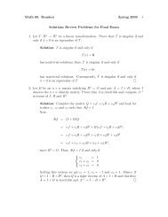
30 CHAPTER 3. RANDOM VARIABLESThere are two kinds of random variables:(1) X is discrete if X takes on values in a finite set, or countable infinite set(that is, a set whose elements can be listed in a sequence x 1 , x 2 , x 3 , . . .)(2) X is continuous if X can take on any value in interval of real numbers.Example 3.1.3 (Discrete Random Variable). Flip a coin three times in a rowand let X denote the number of heads that come up. Then, the possible valuesof X are 0, 1, 2 or 3. Hence, X is discrete.3.2 Distribution FunctionsDefinition 3.2.1 (Probability Mass Function). Given a discrete random variableX defined on a probability space (C, B, Pr), the probability mass function,or pmf, of X is defined byfor all X ∈ R.p(x) = Pr(X = x)Remark 3.2.2. Here we adopt the convention that random variables will bedenoted by capital letters (X, Y , Z, etc.) and their values are denoted by thecorresponding lower case letters (x, x, z, etc.).Example 3.2.3 (Probability Mass Function). Assume the coin in Example3.1.3 is fair. Then, all the outcomes in then sample spaceC = {HHH, HHT, HT H, HT T, T HH, T HT, T T H, T T T }are equally likely. It then follows thatPr(X = 0) = Pr({T T T }) = 1 8 ,andPr(X = 1) = Pr({HT T, T HT, T T H}) = 3 8 ,Pr(X = 2) = Pr({HHT, HT H, T HH}) = 3 8 ,Pr(X = 3) = Pr({HHH}) = 1 8 .We then have that the pmf for X is⎧1/8 if x = 0,⎪⎨ 3/8 if x = 1,p(x) = 3/8 if x = 2,1/8 if x = 0,⎪⎩0 otherwise.A graph of this function is pictured in Figure 3.2.1.

3.2. DISTRIBUTION FUNCTIONS 31p1r r r r1 2 3xFigure 3.2.1: Probability Mass Function for XRemark 3.2.4 (Properties of probability mass functions). In the previous exampleobserve that the values of p(x) are non–negative and add up to 1; thatis, p(x) ⩾ 0 for all x and∑p(x) = 1.We usually just list the values of X for which p(x) is not 0:xp(x 1) p(x 2), . . . , p(x N),in the case in which X takes on a finite number of non–zero values, orp(x 1), p(x 2), p(x 3), . . .if X takes on countably many non–zero values. We then have thatN∑p(x k) = 1k=1in the finite case, andin the countably infinite case.∞∑p(x k) = 1k=1Definition 3.2.5 (Cumulative Distribution Function). Given any random variableX defined on a probability space (C, B, Pr), the cumulative distributionfunction, or cmf, of X is define byfor all X ∈ R.F X(x) = Pr(X ⩽ x)

32 CHAPTER 3. RANDOM VARIABLESExample 3.2.6 (Cumulative Distribution Function). Let (C, B, Pr) and X beas defined in Example 3.2.3. We compute F Xas follows:First observe that if x < 0, then Pr(X ⩽ x) = 0; thus,F X(x) = 0 for all x < 0.Note that p(x) = 0 for 0 < x < 1; it then follows thatF X(x) = Pr(X ⩽ x) = Pr(X = 0) for 0 < x < 1.On the other hand, Pr(X ⩽ 1) = Pr(X = 0)+Pr(X = 1) = 1/8+3/8 = 1/2;thus,F X(1) = 1/2.Next, since p(x) = 0 for all 1 < x < 2, we also get thatF X(x) = 1/2 for 1 < x < 2.Continuing in this fashion we obtain the following formula for F X:⎧0 if x < 0,⎪⎨ 1/8 if 0 ⩽ x < 1,F X(x) = 1/2 if 1 ⩽ x < 2,7/8 if 2 ⩽ x < 3,⎪⎩1 if x ⩾ 3.Figure 3.2.2 shows the graph of F X.F X1rrr r1 2 3xFigure 3.2.2: Cumulative Distribution Function for XRemark 3.2.7 (Properties of Cumulative Distribution Functions). The graphin Figure 3.2.2 illustrates several properties of cumulative distribution functionswhich we will prove later in the course.(1) F Xis non–negative and non–degreasing; that is, F X(x) ⩾ 0 for all x ∈ Rand F X(a) ⩽ F X(b) whenever a < b.

3.2. DISTRIBUTION FUNCTIONS 33(2) lim F (x) = 0 and lim F (x) = 1.X Xx→−∞ x→+∞(3) F Xis right–continuous or upper semi–continuous; that is,lim F (x) = F (a)x→a + X Xfor all a ∈ R. Observe that the limit is taken as x approaches a from theright.Example 3.2.8 (Service time at a checkout counter). Suppose you sit by acheckout counter at a supermarket and measure the time, T , it takes for eachcustomer to be served. This is a continuous random variable that takes on valuesin a time continuum. We would like to compute the cumulative distributionfunction F T(t) = Pr(T ⩽ t), for all t > 0.Let N(t) denote the number of customers being served at a checkout counter(not in line) at time t. Then N(t) = 1 or N(t) = 0. Let p(t) = Pr[N(t) = 1] andassume that p(t) is a differentiable function of t. Assume also that p(0) = 1;that is, at the start of the observation, one person is being served.Consider now p(t + Δt), where Δt is very small; i.e., the probability that aperson is being served at time t + Δt. Suppose that the probability that servicewill be completed in the short time interval [t, t + Δt] is proportional to Δt;say μΔt, where μ > 0 is a proportionality constant. Then, the probability thatservice will not be completed at t + Δt is 1 − μΔt. This situation is illustratedin the state diagram pictured in Figure 3.2.3:# # ¢§¤"! "!1 − μΔt1 0μΔtFigure 3.2.3: State diagram for N(t)The circles in the state diagram represent the possible values of N(t), orstates. In this case, the states are 1 or 0, corresponding to one person beingserved and no person being served, respectively. The arrows represent transitionprobabilities from one state to another (or the same) in the interval from t tot + Δt. Thus the probability of going from sate N(t) = 1 to state N(t) = 0 inthat interval (that is, service is completed) is μΔt, while the probability thatthe person will still be at the counter at the end of the interval is 1 − μΔt.We therefore get thatp(t + Δt) = (probability person is being served at t)(1 − μΔt);

34 CHAPTER 3. RANDOM VARIABLESthat is,orp(t + Δt) = p(t)(1 − μΔt),p(t + Δt) − p(t) = −μΔ + p(t).Dividing by Δt ∕= 0 we therefore get thatp(t = Δt) − p(t)Δt= −μp(t)Thus, letting Δt → 0 and using the the assumption that p is differentiable, wegetdpdt = −μp(t).Sincep(0) = 1, we get p(t) = e −μt for t ⩾ 0.Recall that T denotes the time it takes for service to be completed, or theservice time at the checkout counter. Then, it is the case thatfor all t > 0. Thus,Pr[T > t] = p[N(t) = 1]= p(t)= e −μtPr[T ≤ t] = 1 − e −μtThus, T is a continuous random variable with cdf.F T(t) = 1 − e −μt , t > 0.A graph of this cdf is shown in Figure 3.2.4.1.00.750.50.250.0012x345Figure 3.2.4: Cumulative Distribution Function for TDefinition 3.2.9. Let X denote a continuous random variable such that F X(x)is differentiable. Then, the derivative f T(x) = F ′ (x) is called the probabilityXdensity function, or pdf, of X.

3.2. DISTRIBUTION FUNCTIONS 35Example 3.2.10. In the service time example, Example 3.2.8, if T is the timethat it takes for service to be completed at a checkout counter, then the cdf forT isF T(t) = 1 − e −μt for all t ⩾ 0.Thus,f T(t) = μe −μt , for all t > 0,is the pdf for T , and we say that T follows an exponential distribution withparameter 1/μ. We will see the significance of the parameter μ in the nextchapter.In general, given a function f : R → R, which is non–negative and integrablewith∫ ∞−∞f(x) dx = 1,f defines the pdf for some continuous random variable X. In fact, the cdf forX is defined byF X(x) =∫ x−∞f(t) dt for all x ∈ R.Example 3.2.11. Let a and b be real numbers with a < b. The function⎧1⎪⎨ if a < x < b,b − af(x) =⎪⎩0 otherwise,defines a pdf sinceand f is non–negative.∫ ∞−∞f(x) dx =∫ ba1b − adx = 1,Definition 3.2.12 (Uniform Distribution). A continuous random variable, X,having the pdf given in the previous example is said to be uniformly distributedon the interval (a, b). We writeX ∼ Uniform(a, b).Example 3.2.13 (Finding the distribution for the square of a random variable).Let X ∼ Uniform(−1, 1) and Y = X 2 give the pdf for Y .Solution: Since X ∼ Uniform(−1, 1) its pdf is given by⎧1⎪⎨ if − 1 < x < 1,2f X(x) =⎪⎩0 otherwise.

36 CHAPTER 3. RANDOM VARIABLESWe would like to compute f Y(y) for 0 < y < 1. In order to do this,first we compute the cdf F Y(y) for 0 < y < 1:F Y(y) = Pr(Y ⩽ y), for 0 < y < 1,= Pr(X 2 ⩽ y)= Pr(∣Y ∣ ⩽ √ y)= Pr(− √ y ⩽ X ⩽ √ y)= Pr(− √ y < X ⩽ √ y), since X is continuous,= Pr(X ⩽ √ y) − Pr(X ⩽ − √ y)= F X( √ y) − F x(− √ y).Differentiating with respect to y we then obtain thatf Y(y) = ddy F Y (y)= ddy F X (√ y) − ddy F X (−√ y)= F ′ X (√ y) ⋅by the Chain Rule, so thatd √ y − F′Xdy(−√ y) ddy (−√ y),f Y(y) = f X( √ 1y) ⋅2 √ y + f ′ (−√ 1y)X2 √ y= 1 2 ⋅ 12 √ y + 1 2 ⋅ 12 √ y=12 √ yfor 0 < y < 1. We then have that{12f Y(y) =√ yif 0 < y < 1,0 otherwise.□

Chapter 4Expectation of RandomVariables4.1 Expected Value of a Random VariableDefinition 4.1.1 (Expected Value of a Continuous Random Variable). Let Xbe a continuous random variable with pdf f X. If∫ ∞−∞∣x∣f X(x) dx < ∞,we define the expected value of X, denoted E(X), byE(X) =∫ ∞−∞xf X(x) dx.Example 4.1.2 (Average Service Time). In the service time example, Example3.2.8, we showed that the time, T , that it takes for service to be completed atcheckout counter has an exponential distribution with pdff T(t) ={μe −μt for t > 0,0 otherwise,where μ is a positive constant.37

38 CHAPTER 4. EXPECTATION OF RANDOM VARIABLESObserve that∫ ∞−∞∣t∣f T(t) dt =∫ ∞0tμe −μt dt= limb→∞∫ b0t μe −μt dt[= lim −te −μt − 1 ] bb→∞μ e−μt 0[ 1= limb→∞ μ − be−μb − 1 ]μ e−μb= 1 μ ,where we have used integration by parts and L’Hospital’s rule. It then followsthat∫ ∞−∞∣t∣f T(t) dt = 1 μ < ∞and therefore the expected value of T exists andE(T ) =∫ ∞−∞tf T(t) dt =∫ ∞0tμe −μt dt = 1 μ .Thus, the parameter μ is the reciprocal of the expected service time, or averageservice time, at the checkout counter.Example 4.1.3. Suppose the average service time, or mean service time, ata checkout counter is 5 minutes. Compute the probability that a given personwill spend at least 6 minutes at the checkout counter.Solution: We assume that the service time, T , is exponentiallydistributed with pdf{μe −μt for t > 0,f T(t) =0 otherwise,where μ = 1/5. We then have thatPr(T ⩾ 6) =∫ ∞6f T(t) dt =∫ ∞615 e−t/5 dt = e −6/5 ≈ 0.30.Thus, there is a 30% chance that a person will spend 6 minutes ormore at the checkout counter.□

4.1. EXPECTED VALUE OF A RANDOM VARIABLE 39Definition 4.1.4 (Exponential Distribution). A continuous random variable,X, is said to be exponentially distributed with parameter β > 0, writtenX ∼ Exponential(β),if it has a pdf given by⎧1⎪⎨ β e−x/β for x > 0,f X(x) =⎪⎩0 otherwise.The expected value of X ∼ Exponential(β), for β > 0, is E(X) = β.Definition 4.1.5 (Expected Value of a Discrete Random Variable). Let X bea discrete random variable with pmf p X. If∑∣x∣p X(x) < ∞,we define the expected value of X, denoted E(X), byxE(X) = ∑ xx p X(x).Example 4.1.6. Let X denote the number on the top face of a balanced die.Compute E(X).Solution: In this case the pmf of X is p X(x) = 1/6 for x =1, 2, 3, 4, 5, 6, zero elsewhere. Then,6∑6∑E(X) = kp X(k) = k ⋅ 1 6 = 7 2 = 3.5.k=1k=1□Definition 4.1.7 (Bernoulli Trials). A Bernoulli Trial, X, is a discrete randomvariable that takes on only the values of 0 and 1. The event (X = 1) iscalled a “success”, while (X = 0) is called a “failure.” The probability of asuccess is denoted by p, where 0 < p < 1. We then have that the pmf of X is⎧⎪⎨ 1 − p if x = 0,p X(x) = p if x = 1,⎪⎩0 elsewhere.If a discrete random variable X has this pmf, we writeX ∼ Bernoulli(p),and say that X is a Bernoulli trial with parameter p.

40 CHAPTER 4. EXPECTATION OF RANDOM VARIABLESExample 4.1.8. Let X ∼ Bernoulli(p). Compute E(X).Solution: ComputeE(X) = 0 ⋅ p X(0) + 1 ⋅ p X(1) = p.Definition 4.1.9 (Independent Discrete Random Variable). Two discrete randomvariables X and Y are said to independent if and only ifPr(X = x, Y = y) = Pr(X = x) ⋅ Pr(Y = y)for all values, x, of X and all values, y, of Y .Note: the event (X = x, Y = y) denotes the event (X = x) ∩ (Y = y); that is,the events (X = x) and (Y = y) occur jointly.Example 4.1.10. Suppose X 1 ∼ Bernoulli(p) and X 2 ∼ Bernoulli(p) are independentrandom variables with 0 < p < 1. Define Y 2 = X 1 + X 2 . Find the pmffor Y 2 and compute E(Y 2 ).Solution: Observe that Y 2 takes on the values 0, 1 and 2. WecomputePr(Y 2 = 0) = Pr(X 1 = 0, X 2 = 0)= Pr(X 1 = 0) ⋅ Pr(X 2 = 0), by independence,= (1 − p) ⋅ (1 − p)= (1 − p) 2 .Next, since the event (Y 2 = 1) consists of the disjoint union of theevents (X 1 = 1, X 2 = 0) and (X 1 = 0, X 2 = 1),Pr(Y 2 = 1) = Pr(X 1 = 1, X 2 = 0) + Pr(X 1 = 0, X 2 = 1)= Pr(X 1 = 1) ⋅ Pr(X 2 = 0) + Pr(X 1 = 0) ⋅ Pr(X 2 = 1)= p(1 − p) + (1 − p)p= 2p(1 − p).Finally,Pr(Y 2 = 2) = Pr(X 1 = 1, X 2 = 1)= Pr(X 1 = 1) ⋅ Pr(X 2 = 1)= p ⋅ p= p 2 .We then have that the pmf of Y 2 is given by⎧(1 − p) 2 if y = 0,⎪⎨2p(1 − p) if y = 1,p Y2(y) =p⎪⎩2 if y = 2,0 elsewhere.□

4.1. EXPECTED VALUE OF A RANDOM VARIABLE 41To find E(Y 2 ), computeE(Y 2 ) = 0 ⋅ p Y2(0) + 1 ⋅ p Y2(1) + 2 ⋅ p Y2(2)= 2p(1 − p) + 2p 2= 2p[(1 − p) + p]= 2p.We shall next consider the case in which we add three mutually independentBernoulli trials. Before we present this example, we give a precise definition ofmutual independence.Definition 4.1.11 (Mutual Independent Discrete Random Variable). Threediscrete random variables X 1 , X 2 and X 3 are said to mutually independentif and only if(i) they are pair–wise independent; that is,(ii) andPr(X i = x i , X j = x j ) = Pr(X i = x i ) ⋅ Pr(X j = x j )for all values, x i , of X i and all values, x j , of X j ;□for i ∕= j,Pr(X 1 = x 1 , X 2 = x 2 , X 3 = x 3 ) = Pr(X 1 = x 1 )⋅Pr(X 2 = x 2 )⋅Pr(X 3 = x 3 ).Lemma 4.1.12. Let X 1 , X 2 and X 3 be mutually independent, discrete randomvariables and define Y 2 = X 1 + X 2 . Then, Y 2 and X 3 are independent.Proof: ComputePr(Y 2 = w, X 3 = z) = Pr(X 1 + X 2 = w, X 3 = z)= ∑ xPr(X 1 = x, X 2 = w − x, X 3 = z),where the summation is taken over possible value of X 1 . It then follows thatPr(Y 2 = w, X 3 = z) = ∑ xPr(X 1 = x) ⋅ Pr(X 2 = w − x) ⋅ Pr(X 3 = z),where we have used (ii) in Definition 4.1.11. Thus, by pairwise independence,(i.e., (i) in Definition 4.1.11),( )∑Pr(Y 2 = w, X 3 = z) = Pr(X 1 = x) ⋅ Pr(X 2 = w − x) ⋅ Pr(X 3 = z)x= Pr(X 1 + X 2 = w) ⋅ Pr(X 3 = z)= Pr(Y 2 = w) ⋅ Pr(X 3 = z),which shows the independence of Y 2 and X 3 .

42 CHAPTER 4. EXPECTATION OF RANDOM VARIABLESExample 4.1.13. Suppose X 1 , X 2 and X 3 be three mutually independentBernoulli random variables with parameter p, where 0 < p < 1. Define Y 3 =X 1 + X 2 + X 3 . Find the pmf for Y 3 and compute E(Y 3 ).Solution: Observe that Y 3 takes on the values 0, 1, 2 and 3, andthatY 3 = Y 2 + X 3 ,where the pmf and expected value of Y 2 were computed in Example4.1.10.We computePr(Y 3 = 0) = Pr(Y 2 = 0, X 3 = 0)= Pr(Y 2 = 0) ⋅ Pr(X 3 = 0), by independence (Lemma 4.1.12),= (1 − p) 2 ⋅ (1 − p)= (1 − p) 3 .Next, since the event (Y 3 = 1) consists of the disjoint union of theevents (Y 2 = 1, X 3 = 0) and (Y 2 = 0, X 3 = 1),Pr(Y 3 = 1) = Pr(Y 2 = 1, X 3 = 0) + Pr(Y 2 = 0, X 3 = 1)= Pr(Y 2 = 1) ⋅ Pr(X 3 = 0) + Pr(Y 2 = 0) ⋅ Pr(X 3 = 1)= 2p(1 − p)(1 − p) + (1 − p) 2 p= 3p(1 − p) 2 .Similarly,Pr(Y 3 = 2) = Pr(Y 2 = 2, X 3 = 0) + Pr(Y 2 = 1, X 3 = 1)= Pr(Y 2 = 2) ⋅ Pr(X 3 = 0) + Pr(Y 2 = 1) ⋅ Pr(X 3 = 1)= p 2 (1 − p) + 2p(1 − p)p= 3p 2 (1 − p),andPr(Y 3 = 3) = Pr(Y 2 = 2, X 3 = 1)= Pr(Y 2 = 0) ⋅ Pr(X 3 = 0)= p 2 ⋅ p= p 3 .We then have that the pmf of Y 3 is⎧(1 − p) 3 if y = 0,⎪⎨ 3p(1 − p) 2 if y = 1,p Y3(y) = 3p 2 (1 − p) if y = 2,p 3 if y = 3,⎪⎩0 elsewhere.

4.1. EXPECTED VALUE OF A RANDOM VARIABLE 43To find E(Y 2 ), computeE(Y 2 ) = 0 ⋅ p Y3(0) + 1 ⋅ p Y3(1) + 2 ⋅ p Y3(2) + 3 ⋅ p Y3(3)= 3p(1 − p) 2 + 2 ⋅ 3p 2 (1 − p) + 3p 3= 3p[(1 − p) 2 + 2p(1 − p) + p 2 ]= 3p[(1 − p) + p] 2= 3p.If we go through the calculations in Examples 4.1.10 and 4.1.13 for the case offour mutually independent 1 Bernoulli trials with parameter p, where 0 < p < 1,X 1 , X 2 , X 3 and X 4 , we obtain that for Y 4 = X 1 + X 2 + X 3 + X 4 ,⎧(1 − p) 4 if y = 0,4p(1 − p) 3 if y = 1,⎪⎨6p 2 (1 − p) 2 if y = 2p Y4(y) =4p 3 (1 − p) if y = 3p⎪⎩4 if y = 4,0 elsewhere,andE(Y 4 ) = 4p.Observe that the terms in the expressions for p Y2(y), p Y3(y) and p Y4(y) are theterms in the expansion of [(1 − p) + p] n for n = 2, 3 and 4, respectively. By theBinomial Expansion Theorem,n∑( n[(1 − p) + p] n = pk)k (1 − p) n−k ,k=0where ( n n!=k)k!(n − k)! ,k = 0, 1, 2 . . . , n,are the called the binomial coefficients. This suggests that ifY n = X 1 + X 2 + ⋅ ⋅ ⋅ + X n ,where X 1 , X 2 , . . . , X n are n mutually independent Bernoulli trials with parameterp, for 0 < p < 1, then( np Yn(k) = pk)k (1 − p) n−k for k = 0, 1, 2, . . . , n.Furthermore,E(Y n ) = np.We shall establish this as a the following Theorem:1 Here, not only do we require that the random variable be pairwise independent, but alsothat for any group of k ≥ 2 events (X j = x j ), the probability of their intersection is theproduct of their probabilities.□

44 CHAPTER 4. EXPECTATION OF RANDOM VARIABLESTheorem 4.1.14. Assume that X 1 , X 2 , . . . , X n are mutually independent Bernoullitrials with parameter p, with 0 < p < 1. DefineY n = X 1 + X 2 + ⋅ ⋅ ⋅ + X n .Then the pmf of Y n isp Yn(k) =( nk)p k (1 − p) n−kfor k = 0, 1, 2, . . . , n,andE(Y n ) = np.Proof: We prove this result by induction on n. For n = 1 we have that Y 1 = X 1 ,and thereforep Y1(0) = Pr(X 1 = 0) = 1 − pandp Y1(1) = Pr(X 1 = 1) = p.Thus,⎧⎪⎨ 1 − p if k = 0,p Y1(k) = p if k = 1,⎪⎩0 elsewhere.( ( 1 1Observe that = = 1 and therefore the result holds true for n = 1.0)1)Next, assume the theorem is true for n; that is, suppose that( np Yn(k) = pk)k (1 − p) n−k for k = 0, 1, 2, . . . , n, (4.1)and thatE(Y n ) = np. (4.2)We need to show that the result also holds true for n + 1. In other words,we show that if X 1 , X 2 , . . . , X n , X n+1 are mutually independent Bernoulli trialswith parameter p, with 0 < p < 1, andY n+1 = X 1 + X 2 + ⋅ ⋅ ⋅ + X n + X n+1 , (4.3)then, the pmf of Y n+1 is( ) n + 1p Yn+1(k) = p k (1 − p) n+1−kkfor k = 0, 1, 2, . . . , n, n + 1, (4.4)andFrom (4.5) we see thatE(Y n+1 ) = (n + 1)p. (4.5)Y n+1 = Y n + X n+1 ,

4.1. EXPECTED VALUE OF A RANDOM VARIABLE 45where Y n and X n+1 are independent random variables, by an argument similarto the one in the proof of Lemma 4.1.12 since the X k ’s are mutually independent.Therefore, the following calculations are justified:(i) for k ⩽ n,Pr(Y n+1 = k) = Pr(Y n = k, X n+1 = 0) + Pr(Y n = k − 1, X n+1 = 1)= Pr(Y n = k) ⋅ Pr(X n+1 = 0)+Pr(Y n = k − 1) ⋅ Pr(X n−1 = 1)=( nk)p k (1 − p) n−k (1 − p)( ) n+ p k−1 (1 − p) n−k+1 p,k − 1where we have used the inductive hypothesis (4.1). Thus,Pr(Y n+1 = k) =[( ( )]n n+ pk)k (1 − p) n+1−k .k − 1The expression in (4.4) will following from the fact that( ( )n n+ =k)k − 1( n + 1which can be established by the following counting argument:Imagine n + 1 balls in a bag, n of which are blue and one isred. We consider the collection of all groups of k balls that canbe formed out of the n + 1 balls in the bag. This collection ismade up of two disjoint sub–collections: the ones with the redball and the ones without the red ball. The number of elementsin the collection with the one red ball is( ) nk − 1( 1⋅ =1)k( nk − 1),),while the number of elements in the collection of groups withoutthe red ball are( nk).( ) n + 1Adding these two must yield .k

46 CHAPTER 4. EXPECTATION OF RANDOM VARIABLES(ii) If k = n + 1, thensince k = n + 1.Pr(Y n+1 = k) = Pr(Y n = n, X n+1 = 1)= Pr(Y n = n) ⋅ Pr(X n+1 = 1)= p n p= p n+1=( n + 1k)p k (1 − p) n+1−k ,Finally, to establish (4.5) based on (4.2), use the result of Problem 2 inAssignment 10 to show that, since Y n and X n are independent,E(Y n+1 ) = E(Y n + X n+1 ) = E(Y n ) + E(X n+1 ) = np + p = (n + 1)p.Definition 4.1.15 (Binomial Distribution). Let b be a natural number and0 < p < 1. A discrete random variable, X, having pmf( np X(k) = pk)k (1 − p) n−k for k = 0, 1, 2, . . . , n,is said to have a binomial distribution with parameters n and p.We write X ∼ Binomial(n, p).Remark 4.1.16. In Theorem 4.1.14 we showed that if X ∼ Binomial(n, p),thenE(X) = np.We also showed in that theorem that the sum of n mutually independentBernoulli trials with parameter p, for 0 < p < 1, follows a Binomial distributionwith parameters n and p.Definition 4.1.17 (Independent Identically Distributed Random Variables). Aset of random variables, {X 1 , X 2 , . . . , X n }, is said be independent identicallydistributed, or iid, if the random variables are mutually disjoint and if theyall have the same distribution function.If the random variables X 1 , X 2 , . . . , X n are iid, then they form a simplerandom sample of size n.Example 4.1.18. Let X 1 , X 2 , . . . , X n be a simple random sample from a Bernoulli(p)distribution, with 0 < p < 1. Define the sample mean X byX = X 1 + X 2 + ⋅ ⋅ ⋅ + X n.nGive the distribution function for X and compute E(X).

4.2. LAW OF THE UNCONSCIOUS STATISTICIAN 47Solution: Write Y = nX = X 1 + X 2 + ⋅ ⋅ ⋅ + X n . Then, sinceX 1 , X 2 , . . . , X n are iid Bernoulli(p) random variables, Theorem 4.1.14implies that Y ∼ Binomial(n, p). Consequently, the pmf of Y is( np Y(k) = pk)k (1 − p) n−k for k = 0, 1, 2, . . . , n,and E(Y ) = np.Now, X may take on the values 0, 1 n , 2 n , . . . n − 1 , 1, andnso thatPr(X = x) = Pr(Y = nx) for x = 0, 1 n , 2 n , . . . n − 1n , 1,Pr(X = x) =( nx)p nx (1 − p) n−nx for x = 0, 1 n , 2 n , . . . n − 1n , 1.The expected value of X can be computed as follows( ) 1E(X) = En Y = 1 n E(Y ) = 1 (np) = p.nObserve that X is the proportion of successes in the simple randomsample. It then follows that the expected proportion of successes inthe random sample is p, the probability of a success.□4.2 Law of the Unconscious StatisticianExample 4.2.1. Let X denote a continuous random variable with pdf{3x 2 if 0 < x < 1,f X(x) =0 otherwise.Compute the expected value of X 2 .We show two ways to compute E(X).(i) First Alternative. Let Y = X 2 and compute the pdf of Y . To do this, firstwe compute the cdf:F Y(y) = Pr(Y ⩽ y), for 0 < y < 1,= Pr(X 2 ⩽ y)= Pr(∣X∣ ⩽ √ y)= Pr(− √ y ⩽ ∣X∣ ⩽ √ y)= Pr(− √ y < ∣X∣ ⩽ √ y), since X is continuous,= F X( √ y) − F X(− √ y)= F X( √ y),

48 CHAPTER 4. EXPECTATION OF RANDOM VARIABLESsince f Xis 0 for negative values.It then follows thatf Y(y) = F ′ X (√ y) ⋅= f X( √ y) ⋅= 3( √ y) 2 ⋅ddy (√ y)12 √ y12 √ y= 3 y2√for 0 < y < 1.Consequently, the pdf for Y is⎧⎨3√ y if 0 < y < 1,f Y(y) = 2⎩ 0 otherwise.Therefore,E(X 2 ) = E(Y )==∫ ∞−∞∫ 10yf Y(y) dyy 3 2√ y dy= 3 2∫ 10y 3/2 dy= 3 2 ⋅ 2 5= 3 5 .(ii) Second Alternative. Alternatively, we could have compute E(X 2 ) by evaluating∫ ∞x 2 f X(x) dx =∫ 1−∞0= 3 5 .x 2 ⋅ 3x 2 dx

4.2. LAW OF THE UNCONSCIOUS STATISTICIAN 49The fact that both ways of evaluating E(X 2 ) presented in the previousexample is a consequence of the so–called Law of the Unconscious Statistician:Theorem 4.2.2 (Law of the Unconscious Statistician, Continuous Case). LetX be a continuous random variable and g denote a continuous function definedon the range of X. Then, if∫ ∞−∞E(g(X)) =∣g(x)∣f X(x) dx < ∞,∫ ∞−∞g(x)f X(x) dx.Proof: We prove this result for the special case in which g is differentiable withg ′ (x) > 0 for all x in the range of X. In this case g is strictly increasing and ittherefore has an inverse function g −1 mapping onto the range of X and whichis also differentiable with derivative given byd [g −1 (y) ] = 1dyg ′ (x) = 1g ′ (g −1 (y)) ,where we have set y = g(x) for all x is the range of X, or Y = g(X). Assumealso that the values of X range from −∞ to ∞ and those of Y also range from−∞ to ∞. Thus, using the Change of Variables Theorem, we have that∫ ∞−∞g(x)f X(x) dx =since x = g −1 (y) and thereforeOn the other hand,∫ ∞−∞yf X(g −1 (y)) ⋅dx = d [g −1 (y) ] 1dy =dyg ′ (g −1 (y)) dy.F Y(y) = Pr(Y ⩽ y)= Pr(g(X) ⩽ y)= Pr(X ⩽ g −1 (y))= F X(g −1 (y)),from which we obtain, by the Chain Rule, thatConsequently,or∫ ∞−∞f Y(y) = f X(g −1 1(y)g ′ (g −1 (y)) .yf Y(y) dy =E(Y ) =∫ ∞−∞∫ ∞−∞g(x)f X(x) dx,g(x)f X(x) dx.1g′(g −1 (y)) dy,

50 CHAPTER 4. EXPECTATION OF RANDOM VARIABLESThe law of the unconscious statistician also applies to functions of a discreterandom variable. In this case we haveTheorem 4.2.3 (Law of the Unconscious Statistician, Discrete Case). Let Xbe a discrete random variable with pmf p X, and let g denote a function definedon the range of X. Then, if∑∣g(x)∣p X(x) < ∞,xE(g(X)) = ∑ xg(x)p X(x).4.3 MomentsThe law of the unconscious statistician can be used to evaluate the expectedvalues of powers of a random variableE(X m ) =∫ ∞−∞in the continuous case, provided that∫ ∞−∞In the discrete case we havex m f X(x) dx, m = 0, 1, 2, 3, . . . ,∣x∣ m f X(x) dx < ∞, m = 0, 1, 2, 3, . . . .E(X m ) = ∑ xx m p X(x), m = 0, 1, 2, 3, . . . ,provided that∑∣x∣ m p X(x) < ∞, m = 0, 1, 2, 3, . . . .xDefinition 4.3.1 (mth Moment of a Distribution). E(X m ), if it exists, is calledthe mth moment of X for m = 0, 2, 3, . . .Observe that the first moment of X is its expectation.Example 4.3.2. Let X have a uniform distribution over the interval (a, b) fora < b. Compute the second moment of X.Solution: Using the law of the unconscious statistician we getwhereE(X 2 ) =∫ ∞−∞x 2 f X(x) dx,⎧1⎪⎨ if a < x < b,b − af X(x) =⎪⎩0 otherwise.

4.3. MOMENTS 51Thus,E(X 2 ) ===∫ bax 2b − a dx[ 1b − ax 3 ] b3a13(b − a) ⋅ (b3 − a 3 )= b2 + ab + a 2.3□4.3.1 Moment Generating FunctionUsing the law of the unconscious statistician we can also evaluate E(e tX ) wheneverthis expectation is defined.Example 4.3.3. Let X have an exponential distribution with parameter λ > 0.Determine the values of t ∈ R for which E(e tX ) is defined and compute it.Solution: The pdf of X is given by⎧1⎪⎨λ e−x/λ if x > 0,f X(x) =⎪⎩0 if x ⩽ 0.Then,E(e tX ) =∫ ∞−∞e tx f X(x) dx= 1 λ= 1 λ∫ ∞0∫ ∞0e tx e −x/λ dxe −[(1/λ)−t]x dx.We note that for the integral in the last equation to converge, wemust require thatt < 1/λ.For these values of t we get thatE(e tX ) = 1 λ ⋅ 1(1/λ) − t=11 − λt .

52 CHAPTER 4. EXPECTATION OF RANDOM VARIABLESDefinition 4.3.4 (Moment Generating Function). Given a random variable X,the expectation E(e tX ), for those values of t for which it is defined, is called themoment generating function, or mgf, of X, and is denoted by ψ X(t). Wethen have thatψ X(t) = E(e tX ),whenever the expectation is defined.Example 4.3.5. If X ∼ Exponential(λ), for λ > 0, then Example 4.3.3 showsthat the mgf of X is given by□ψ X(t) = 11 − λtfor t < 1 λ .Example 4.3.6. Let X ∼ Binomial(n, p), for n ⩾ 1 and 0 < p < 1. Computethe mgf of X.Solution: The pmf of X is( np X(k) = pk)k (1 − p) n−kfor k = 0, 1, 2, . . . , n,and therefore, by the law of the unconscious statistician,ψ X(t) = E(e tX )===n∑e tk p X(k)k=1n∑( ) n(e t ) k p k (1 − p) n−kkk=1n∑k=1( nk)(pe t ) k (1 − p) n−k= (pe t + 1 − p) n ,where we have used the Binomial Theorem.We therefore have that if X is binomially distributed with parametersn and p, then its mgf is given byψ X(t) = (1 − p + pe t ) n for all t ∈ R.□

4.3. MOMENTS 534.3.2 Properties of Moment Generating FunctionsFirst observe that for any random variable X,ψ X(0) = E(e 0⋅X ) = E(1) = 1.The importance of the moment generating function stems from the fact that,if ψ X(t) is defined over some interval around t = 0, then it is infinitely differentiablein that interval and its derivatives at t = 0 yield the moments of X.More precisely, in the continuous cases, the m–the order derivative of ψ Xat tis given byψ (m) (t) =∫ ∞−∞x m e tx f X(x) dx, for all m = 0, 1, 2, 3, . . . ,and all t in the interval around 0 where these derivatives are defined. It thenfollows thatψ (m) (0) =∫ ∞−∞x m f X(x) dx = E(X m ), for all m = 0, 1, 2, 3, . . . .Example 4.3.7. Let X ∼ Exponential(λ). Compute the second moment of X.Solution: From Example 4.3.5 we have thatψ X(t) = 11 − λtDifferentiating with respect to t we obtainandψ ′ X (t) =for t < 1 λ .λ(1 − λt) 2 for t < 1 λψ ′′ X (t) = 2λ 2(1 − λt) 3 for t < 1 λ .It then follows that E(X 2 ) = ψ ′′ X (0) = 2λ2 .□Example 4.3.8. Let X ∼ Binomial(n, p). Compute the second moment of X.Solution: From Example 4.3.6 we have thatψ X(t) = (1 − p + pe t ) n for all t ∈ R.Differentiating with respect to t we obtainandψ ′ X (t) = npet (1 − p + pe t ) n−1ψ ′′ X (t) = npet (1 − p + pe t ) n−1 + npe t (n − 1)pe t (1 − p + pe t ) n−2= npe t (1 − p + pe t ) n−1 + n(n − 1)p 2 e 2t (1 − p + pe t ) n−2It then follows that E(X 2 ) = ψ ′′ X (0) = np + n(n − 1)p2 .□

54 CHAPTER 4. EXPECTATION OF RANDOM VARIABLES4.4 VarianceGiven a random variable X for which an expectation exists, defineμ = E(X).μ is usually referred to as the mean of the random variable X.m = 1, 2, 3, . . ., if E(∣X − μ∣ m ) < ∞,E[(X − μ) m ]For givenis called the mth central moment of X. The second central moment of X,E[(X − μ) 2 ],if it exists, is called the variance of X and is denoted by var(X). We then havethatvar(X) = E[(X − μ) 2 ],provided that the expectation is finite. The variance of X measures the averagesquare deviation of the distribution of X from its mean. Thus,√E[(X − μ)2 ]is measure or deviation from the mean. It is usually denoted by σ and is calledthe standard deviation form the mean. We then havevar(X) = σ 2 .We can compute the variance of a random variable X as follows:var(X) = E[(X − μ) 2 ]= E(X 2 − 2μX + μ 2 )= E(X 2 ) − 2μE(X) + μ 2 E(1))= E(X 2 ) − 2μ ⋅ μ + μ 2= E(X 2 ) − μ 2 .Example 4.4.1. Let X ∼ Exponential(λ). Compute the variance of X.Solution: In this case μ = E(X) = λ and, from Example 4.3.7,E(X 2 )2λ 2 . Consequently,var(X) = E(X 2 ) − μ 2 = 2λ 2 − λ 2 = λ 2 .Example 4.4.2. Let X ∼ Binomial(n, p). Compute the variance of X.Solution: Here, μ = np and, from Example 4.3.8, E(X 2 ) = np +n(n − 1)p 2 . Thus,var(X) = E(X 2 ) − μ 2 = np + n(n − 1)p 2 − n 2 p 2 = np(1 − p).□□

Chapter 5Joint DistributionsWhen studying the outcomes of experiments more than one measurement (randomvariable) may be obtained. For example, when studying traffic flow, wemight be interested in the number of cars that go past a point per minute, aswell as the mean speed of the cars counted. We might also be interested inthe spacing between consecutive cars, and the relative speeds of the two cars.For this reason, we are ”interested” in probability statements concerning two ormore random variables.5.1 Definition of Joint DistributionIn order to deal with probabilities for events involving more than one randomvariable, we need to define their joint distribution. We begin with the caseof two random variables X and Y .Definition 5.1.1 (Joint cumulative distribution function). Given random variablesX and Y , the joint cumulative distribution function of X and Y isdefined byF (X,Y )(x, y) = Pr(X ⩽ y, Y ⩽ y) for all (x, y) ∈ R 2 .When both X and Y are discrete random variables, it is more convenient totalk about the joint probability mass function of X and Y :p (X,Y )(x, y) = Pr(X = x, Y = y).We have already talked about the joint distribution of two discrete randomvariables in the case in which they are independent. Here is an example in whichX and Y are not independent:Example 5.1.2. Suppose three chips are randomly selected from a bowl containing3 red, 4 white, and 5 blue chips.55

56 CHAPTER 5. JOINT DISTRIBUTIONSLet X denote the number of red chips chosen, and Y be the number of whitechips chosen. We would like to compute the joint probability function of X andY ; that is,Pr(X = x, Y = y),were x and y range over 0, 1, 2 and 3.For instance,Pr(X = 0, Y = 0) =Pr(X = 0, Y = 1) =Pr(X = 1, Y = 1) =( 5( 3)12) = 10220 = 1 22 ,3) (⋅5( 2)12) = 40220 = 211 ,3) (⋅5( 1)12) = 60220 = 311 ,3( 41( 3) (1 ⋅ 41and so on for all 16 of the joint probabilities. These probabilities are more easilyexpressed in tabular form:X∖Y 0 1 2 3 Row Sums0 1/22 2/11 3/22 2/110 21/551 3/22 3/11 9/110 0 27/552 3/42 3/55 0 0 27/2203 1/220 0 0 0 1/220Column Sums 14/55 28/55 12/55 1/55 1Table 5.1: Joint Probability Distribution for X and Y , p (X,Y )Notice that pmf’s for the individual random variables X and Y can beobtained as follows:3∑p X(i) = P (i, j) ← adding up i th rowfor i = 1, 2, 3, andp Y(j) =j=03∑P (i, j) ← adding up j th columni=0for j = 1, 2, 3.These are expressed in Table 5.1 as “row sums” and “column sums,” respectively,on the “margins” of the table. For this reason p Xand p Yare usuallycalled marginal distributions.Observe that, for instance,0 = Pr(X = 3, Y = 1) ∕= p X(3) ⋅ p Y(2) = 1220 ⋅ 2855 ,and therefore X and Y are not independent.

5.1. DEFINITION OF JOINT DISTRIBUTION 57Definition 5.1.3 (Joint Probability Density Function). An integrable functionf : R 2 → R is said to be a joint pdf of the continuous random variables X andY iff(i) f(x, y) ⩾ 0 for all (x, y) ∈ R 2 , and(ii)∫ ∞ ∫ ∞−∞−∞f(x, y) dxdy = 1.Example 5.1.4. Consider the disk of radius 1 centered at the origin,D 1 = {(x, y) ∈ R 2 ∣ x 2 + y 2 < 1}.The uniform joint distribution for the disc is given by the function⎧1⎪⎨ if x 2 + y 2 < 1,πf(x, y) =⎪⎩0 otherwise.This is the joint pdf for two random variables, X and Y , since∫ ∞ ∫ ∞∫∫1f(x, y) dxdy =−∞ −∞D 1π dxdy = 1 π ⋅ area(D 1) = 1,since area(D 1 ) = π.This pdf models a situation in which the random variables X and Y denotethe coordinates of a point on the unit disk chosen at random.If X and Y are continuous random variables with joint pdf f (X,Y ), then thejoint cumulative distribution function, F (X,Y ), is given byF (X,Y )(x, y) = Pr(X ≤ x, Y ≤ y) =∫ x−∞∫ y−∞f (X,Y )(u, v) dudv,for all (x, y) ∈ R 2 .Given the joint pdf, f (X,Y ), of two random variables defined on the samesample space, C, we can compute the probability of events of the form((X, Y ) ∈ A) = {c ∈ C ∣ (X(c), Y (c)) ∈ A},where A is a Borel subset 1 of R 2 , is compyted as follows∫∫Pr((X, Y ) ∈ A) = f (X,Y )(x, y) dxdy.1 Borel sets in R 2 are generated by bounded open disks; i.e, the setswhere (x o, y o) ∈ R 2 and r > 0.{(x, y) ∈ R 2 ∣ (x − x o) 2 + (y − y o) 2 < r 2 },A

58 CHAPTER 5. JOINT DISTRIBUTIONSExample 5.1.5. A point is chosen at random from the open unit disk D 1 .Compute the probability that that the sum of its coordinates is bigger than 1.Solution: Let (X, Y ) denote the coordinates of a point drawn atrandom from the unit disk D 1 = {(x, y) ∈ R 2 ∣ x 2 + y 2 < 1}. Thenthe joint pdf of X and Y is the one given in Example 5.1.4; that is,⎧1⎪⎨ if x 2 + y 2 < 1,πf (X,Y )(x, y) =⎪⎩0 otherwise.We wish to compute Pr(X + Y > 1). This is given by∫∫Pr(X + Y > 1) = f (X,Y )(x, y) dxdy,AwhereA = {(x, y) ∈ R 2 ∣ x 2 + y 2 < 1, x + y > 1}.The set A is sketched in Figure 5.1.1.y'$A1&%1 xFigure 5.1.1: Sketch of region APr(X + Y > 1) =∫∫A1π dxdy= 1 π area(A)= 1 π( π4 − 1 2)= 1 4 − 12π ≈ 0.09,Since the area of A is the area of one quarter of that of the diskminus the are of the triangle with vertices (0, 0), (1, 0) and (0, 1). □

5.2. MARGINAL DISTRIBUTIONS 595.2 Marginal DistributionsWe have seen that if X and Y are discrete random variables with joint pmfp (X,Y ), then the marginal distributions are given byp X(x) = ∑ yp (X,Y )(x, y),andp Y(y) = ∑ xp (X,Y )(x, y),where the sums are taken over all possible values of y and x, respectively.We can define marginal distributions for continuous random variables X andY from their joint pdf in an analogous way:andf X(x) =f Y(y) =∫ ∞−∞∫ ∞−∞f (X,Y )(x, y) dyf (X,Y )(x, y)dx.Example 5.2.1. Let X and Y have joint pdf given by⎧1⎪⎨ if x 2 + y 2 < 1,πf (X,Y )(x, y) =⎪⎩0 otherwise.Then, the marginal distribution of X is given byf X(x) =and∫ ∞−∞f (X,Y )(x, y) dy = 1 π∫ √ 1−x 2− √ 1−x 2dy = 2 πf X (x) = 0 for ∣x∣ ⩾ 1.'$y1y = √ 1 − x 2&%1 xy = − √ 1 − x 2√1 − x2 for − 1 < x < 1Similarly,⎧2 √⎪⎨ 1 − y2if ∣y∣ < 1πf Y (y) =⎪⎩0 if ∣y∣ ⩾ 1.

60 CHAPTER 5. JOINT DISTRIBUTIONS'$y1x = − √ 1 − y x = √ 21 − y 2&%1 xObserve that, in the previous example,f (X,Y )(x, y) ∕= f X (x) ⋅ f Y (y),sinceSince 1 π ∕= 4 π 2 √1 − x2 √ 1 − y 2 ,for (x, y) in the unit disk. We then say that X and Y are not independent.Example 5.2.2. Let X and Y denote the coordinates of a point selected atrandom from the unit disc and set Z = √ X 2 + Y 2Compute the cdf for Z, F Z(z) for 0 < z < 1 and the expectation of Z.Solution: The joint pdf of X and Y is given by⎧1⎪⎨ if x 2 + y 2 < 1,πf (X,Y )(x, y) =⎪⎩0 otherwise.Pr(Z ⩽ z) = Pr(X 2 + Y 2 ⩽ z 2 ), for 0 < z < 1,=∫∫= 1 πX 2 +Y 2 ⩽z 2 f (X,Y )(x, y) dy dx∫ 2π ∫ z0= 1 π (2π)r2 2= z 2 ,0∣∣ z 0r drdθwhere we changed to polar coordinates. Thus,F Z(z) = z 2 for 0 < z < 1.Consequently,f Z(z) ={2z if 0 < z < 1,0 otherwise.

5.2. MARGINAL DISTRIBUTIONS 61Thus, computing the expectation,E(Z) ===∫ ∞−∞∫ 10∫ 10zf Z(z) dzz(2z) dz2z 2 dz = 2 3 .Observe that we could have obtained the answer in the previous example bycomputingE(D) = E( √ X 2 + Y 2 )==∫∫√x2 + y 2 f (X,Y )(x, y) dxdyR 2∫∫√x2 + y 2 1 π dxdy,Awhere A = {(x, y) ∈ R 2 ∣ x 2 + y 2 < 1}. Thus, using polar coordinates again, weobtainE(D) = 1 π∫ 2π ∫ 10= 1 ∫ 1π 2π r 2 dr= 2 3 .00r rdrdθThis is, again, the “law of the unconscious statistician;” that is,∫∫E[g(X, Y )] = g(x, y)f (X,Y )(x, y) dxdy,R 2for any integrable function g of two variables for which∫∫R 2 ∣g(x, y)∣f (X,Y )(x, y) dxdy < ∞.Theorem 5.2.3. Let X and Y denote continuous random variable with jointpdf f (X,Y ). Then,E(X + Y ) = E(X) + E(Y ).□

62 CHAPTER 5. JOINT DISTRIBUTIONSIn this theorem,E(X) =andE(Y ) =∫ ∞−∞∫ ∞−∞xf X(x) dx,yf Y(x) dy,where f Xand f Yare the marginal distributions of X and Y , respectively.Proof of Theorem.E(X + Y ) =====∫∫(x + y)f (X,Y )R 2 dxdy∫∫∫∫xf (X,Y )dxdy +R 2 yf (X,Y )R 2 dxdy∫ ∞ ∫ ∞−∞∫ ∞−∞∫ ∞−∞−∞∫ ∞ ∫ ∞xf (X,Y )dydx + yf (X,Y )dxdy−∞ −∞∫ ∞x f (X,Y )dydx +−∞∫ ∞−∞∫ ∞xf X(x) dx + yf Y(y) dy−∞∫ ∞y f (X,Y )dxdy−∞= E(X) + E(Y ).5.3 Independent Random VariablesTwo random variables X and Y are said to be independent if for any events Aand B in R (e.g., Borel sets),Pr((X, Y ) ∈ A × B) = Pr(X ∈ A) ⋅ Pr(Y ∈ B),where A × B denotes the Cartesian product of A and B:A × B = {(x, y) ∈ R 2 ∣ x ∈ A and x ∈ B}.In terms of cumulative distribution functions, this translates intoF (X,Y )(x, y) = F X(x) ⋅ F Y(y) for all (x, y) ∈ R 2 . (5.1)We have seen that, in the case in which X and Y are discrete, independence ofX and Y is equivalent top (X,Y )(x, y) = p X(x) ⋅ p Y(y) for all (x, y) ∈ R 2 .

5.3. INDEPENDENT RANDOM VARIABLES 63For continuous random variables we have the analogous expression in terms ofpdfs:f (X,Y )(x, y) = f X(x) ⋅ f Y(y) for all (x, y) ∈ R 2 . (5.2)This follows by taking second partial derivatives on the expression (5.1) for thecdfs sincef (X,Y )(x, y) = ∂2 F (X,Y )(x, y)∂x∂yfor points (x, y) at which f (X,Y )is continuous, by the Fundamental Theorem ofCalculus.Hence, knowing that X and Y are independent and knowing the correspondingmarginal pdfs, in the case in which X and Y are continuous, allows us tocompute their joint pdf by using Equation (5.2).Example 5.3.1. A line segment of unit length is divided into three pieces byselecting two points at random and independently and then cutting the segmentat the two selected pints. Compute the probability that the three pieces willform a triangle.Solution: Let X and Y denote the the coordinates of the selectedpoints. We may assume that X and Y are uniformly distributedover (0, 1) and independent. We then have that{{1 if 0 < x < 1,1 if 0 < y < 1,f X(x) =and f Y(y) =0 otherwise,0 otherwise.Consequently, the joint distribution of X and Y is{1 if 0 < x < 1, 0 < y < 1,f (X,Y )= f X(x) ⋅ f Y(y) =0 otherwise.If X < Y , the three pieces of length X, Y − X and 1 − Y will forma triangle if and only if the following three conditions derived fromthe triangle inequality hold (see Figure 5.3.2): 1 − Y X Y − XFigure 5.3.2: Random TriangleX ⩽ Y − X + 1 − Y ⇒ X ⩽ 1/2,

64 CHAPTER 5. JOINT DISTRIBUTIONSandY − X ⩽ X + 1 − Y ⇒ Y ⩽ X + 1/2,1 − Y ⩽ X + Y − X ⇒ Y ⩾ 1/2.Similarly, if X > Y , a triangle is formed ifY ⩽ 1/2,andY ⩾ X − 1/2,X ⩾ 1/2.Thus, the event that a triangle is formed is the disjoint union of theeventsandA 1 = (X < Y, X ⩽ 1/2, Y ⩽ X + 1/2, Y ⩾ 1/2)A 2 = (X > Y, Y ⩽ 1/2, Y ⩾ X − 1/2, X ⩾ 1/2).These are pictured in Figure 5.3.3:y y = x A 1 A 2 0.5 1 xFigure 5.3.3: Sketch of events A 1 and A 2

5.3. INDEPENDENT RANDOM VARIABLES 65We then have thatPr(triangle) = Pr(A 1 ∪ A 2 )=∫∫f (X,Y )(x, y) dxdyA 1∪A 2∫∫=dxdyA 1∪A 2= area(A 1 ) + area(A 2 )= 1 4 .Thus, there is a 25% chance that the three pieces will form a triangle.□Example 5.3.2 (Buffon’s Needle Experiment). An experiment consists of droppinga needle of unit length onto a table that has a grid of parallel lines one unitdistance apart from one another (see Figure 5.3.4). Compute the probabilitythat the needle will cross one of the lines.qX θFigure 5.3.4: Buffon’s Needle ExperimentSolution: Let X denote the distance from the mid–point of theneedle to the closest line (see Figure 5.3.4). We assume that X isuniformly distributed on (0, 1/2); thus, the pdf of X is:{2 if 0 < x < 1/2,f X(x) =0 otherwise.Let Θ denote the acute angle that the needle makes with a lineperpendicular to the parallel lines. We assume that Θ and X are

66 CHAPTER 5. JOINT DISTRIBUTIONSindependent and that Θ is uniformly distributed over (0, π/2). Then,the pdf of Θ is given by⎧2⎪⎨ if 0 < θ < π/2,πf Θ(θ) =⎪⎩0 otherwise,and the joint pdf of X and Θ is⎧4⎪⎨ if 0 < x < 1/2, 0 < θ < π/2,πf (X,Θ)(x, θ) =⎪⎩0 otherwise.When the needle meets a line, as shown in Figure 5.3.4, it makesa right triangle with the line it meets and the segment of length XXshown in the Figure. Then, is the length of the hypothenusecos θof that triangle. We therefore have that the event that the needlewill meet a line is equivalent to the eventorA =Xcos Θ < 1 2 ,{(x, θ) ∈ (0, 2) × (0, π/2) ∣ X < 1 }2 cos θ .We then have that the probability that the needle meets a line is∫∫Pr(A) = f (X,Θ)(x, θ) dxdθA=∫ π/2 ∫ cos(θ)/2004π dxdθ= 2 π∫ π/20= 2 π sin θ ∣ ∣∣π/2= 2 π .0cos θ dθThus, there is a 2/π, or about 64%, chance that the needle will meeta line.□Example 5.3.3 (Infinite two–dimensional target). Place the center of a targetfor a darts game at the origin of the xy–plane. If a dart lands at a point with

5.3. INDEPENDENT RANDOM VARIABLES 67yr(X, Y )rxFigure 5.3.5: xy–targetcoordinates (X, Y ), then the random variables X and Y measure the horizontaland vertical miss distance, respectively. For instance, if X < 0 and Y > 0 , thenthe dart landed to the left of the center at a distance ∣X∣ from a vertical linegoing through the origin, and at a distance Y above the horizontal line goingthrough the origin (see Figure 5.3.5).We assume that X and Y are independent, and we are interested in findingthe marginal pdfs f Xand f Yof X and Y , respectively.Assume further that the joint pdf of X and Y is given by the functionf(x, y), and that it depends only on the distance from (X, Y ) to the origin.More precisely, we suppose thatf(x, y) = g(x 2 + y 2 ) for all (x, y) ∈ R 2 ,where g is a differentiable function of a single variable. This implies thatandg(t) ⩾ 0 for all t ⩾ 0,∫ ∞This follows from the fact that f is a pdf and therefore∫∫R 2 f(x, y) dxdy = 1.Thus, switching to polar coordinates,1 =0g(t) dt = 1 π . (5.3)∫ 2π ∫ ∞00g(r 2 )r ddθ.

68 CHAPTER 5. JOINT DISTRIBUTIONSHence, after making the change of variables t = r 2 , we get that1 = 2π∫ ∞0g(r 2 ) rdr = π∫ ∞0g(t) dt,from which (5.3) follows.Now, since X and Y are independent, it follows thatThusf(x, y) = f X(x) ⋅ f Y(y) for all (x, y) ∈ R 2 .f X (x) ⋅ f Y (y) = g(x 2 + y 2 ).Differentiating with respect to x, we getf ′ X (x) ⋅ f Y (y) = g′ (x 2 + y 2 ) ⋅ 2x.Dividing this equation by x ⋅ f X(x) ⋅ f Y(y) = x ⋅ g(x 2 + y 2 ), we get1x ⋅ f ′ (x) Xf X(x) = 2g′ (x 2 + y 2 )g(x 2 + y 2 )for all (x, y) ∈ R 2with (x, y) ∕= (0, 0).Observe that the left–hand side of the equation is a function of x, while theright hand side is a function of both x and y. It follows that the left-hand-sidemust be constant. The reason for this is that, by symmetry,So that,2 g′ (x 2 + y 2g(x 2 + y 2 ) = 1 f ′ (y) Yy f Y(y)1 f ′ (x) Xx f X(x) = 1 f ′ (y) Yy f Y(y)for all (x, y) ∈ R 2 , (x, y) ∕= (0, 0. Thus, in particular1 f ′ (x) Xx f X(x) = f ′ (1) Y= a, for all x ∈ R,f Y(1)and some constant a. It then follows thatfor all x ∈ R. We therefore get thatf ′ X (x)f X(x) = axd [ln(fX (x)) ] = ax.dxIntegrating with respect to x, we then have thatln ( f X(x) ) = a x22 + c 1,

5.3. INDEPENDENT RANDOM VARIABLES 69for some constant of integration c 1 . Thus, exponentiating on both sides of theequation we get thatf X(x) = ce a 2 x2 for all x ∈ R.Thus f X(x) must be a multiple of e a 2 x2 . Now, for this to be a pdf, we must havethat∫ ∞−∞f X(x) dx = 1.Then, necessarily, it must be the case that a < 0 (Why?). Say, a = −δ 2 , thenf X(x) = ce − δ2 2 x2To determine what the constant c should be, we use the conditionLetObserve thatWe then have thatI 2 ==∫ ∞I =I =∫ ∞−∞f X(x) dx = 1.∫ ∞−∞∫ ∞−∞−∞∫ ∞ ∫ ∞−∞e −δ2 x 2 /2 dx.e −δ2 y 2 /2 dy.∫ ∞x2 −δ2e 2 dx ⋅−∞Switching to polar coordinates we gete −δ2 y2 2−∞e −δ22 (x2 +y 2) dxdy.dyI 2 =∫ 2π ∫ ∞e − δ2 2 r20 0= 2π ∫ ∞δ 2 e −u du= 2πδ 2 ,0r drdθwhere we have also made the change of variables u = δ22 r2 . Thus, taking thesquare root,√2πI =δ .Hence, the condition∫ ∞−∞f X(x)dx = 1

70 CHAPTER 5. JOINT DISTRIBUTIONSimplies thatfrom which we get that√2πc = 1δc =δ √2πThus, the pdf for X isf X(x) =δ √2πe − δ2 x 22 for all x ∈ R.Similarly, or by using symmetry, we obtain that the pdf for Y isf Y(y) =δ √2πe − δ2 y 22 for all y ∈ R.That is, X and Y have the same distribution.We next set out to compute the expected value and variance of X. In orderto do this, we first compute the moment generating function, ψ X(t), of X:ψ X(t) = E ( e tX)===Complete the square on x to getthen,∫δ ∞√2π−∞∫δ ∞√2π−∞∫δ ∞√2π−∞e tx e −δ2 x 22 dxe − δ2 x 22 +tx dxe − δ2 2 (x2 − 2txδ 2 ) dxx 2 − 2tδ 2 x = x2 − 2t(t2x +δ2 δ 4 − t2δ 4 = x − t ) 2δ 2 − t2δ 4 ;ψ X(t) =Make the change of variablesthen du = dx and∫δ ∞√2πe − δ2 2−∞= e t2 /2δ 2 δ √2π∫ ∞ψ X(t) = e t22δ 2= e t22δ 2 ,u = x − tδ 2(x− tδ 2 )2 e t2 /2δ 2dxe − δ2 2−∞∫δ ∞√2π−∞(x− tδ 2 ) dx.e −δ22 u2 du

5.3. INDEPENDENT RANDOM VARIABLES 71since, as we have previously seen in this example,f(u) =δ √2πe −δ22 u2 , for u ∈ R,is a pdf and thereforeHence, the mgf of X is∫ ∞−∞δ√2πe −δ22 u2 du = 1.ψ X(t) = e t22δ 2 for all t ∈ R.Differentiating with respect to t we obtainandfor all t ∈ R.ψ ′ Xt t2(t) = e 2δδ2 2ψ ′′ X (t) = 1 δ 2 (1 + t2δ 2 )e t2 /2δ 20.40.30.20.10.0−4−2024xFigure 5.3.6: pdf for X ∼ Normal(0, 25/8π)Hence, the mean value of X isE(X) = ψ ′ X (0) = 0

72 CHAPTER 5. JOINT DISTRIBUTIONSand the second moment of X isE(X 2 ) = ψ ′′ X (0) = 1 δ 2 .Thus, the variance of X isvar(X) = 1 δ 2 .Next, set σ 2 = var(X). We then have thatσ = 1 δ ,and we therefore can write the pdf of X asf X(x) = 1 √2πσe − x22σ 2 − ∞ < x < ∞.A continuous random variable X having the pdff X(x) = 1 √2πσe − x22σ 2 , for − ∞ < x < ∞,is said to have a normal distribution with mean 0 and variance σ 2 . We writeX ∼ Normal(0, σ 2 ). Similarly, Y ∼ Normal(0, σ 2 ). A graph of the pdf forX ∼ Normal(0, σ 2 ), for σ = 5/ √ 8π, is shown in Figure 5.3.6

Chapter 6Some Special DistributionsIn this notes and in the exercises we have encountered several special kindsof random variables and their respective distribution functions in the contextof various examples and applications. For example, we have seen the uniformdistribution over some interval (a, b) in the context of medeling the selection ofa point in (a, b) at random, and the exponential distribution comes up whenmodeling the service time at a checkout counter. We have discussed Bernoullitrials and have seen that the sum of independent Bernoulli trials gives rise tothe Binomial distribution. In the exercises we have seen the discrete uniformdistribution, the geometric distribution and the hypergeometric distribution.More recently, in the last example of the previous section, we have seen thethe miss horizontal distance from the y–axis of dart that lands in an infinitetarget follows a Normal(0, σ 2 ) distribution (assuming that the miss horizontaland vertical distances are independent and that their joint pdf is radially symmetric).In the next section we discuss the normal distribution in more detail.In subsequent sections we discuss other distributions which come up frequentlyin application, such as the Poisson distribution.6.1 The Normal DistributionIn Example 5.3.3 we saw that if X denotes the horizontal miss distance fromthe y–axis of a dart that lands on an infinite two–dimensional target, the X hasa pdf given byf X(x) = 1 √2πσe − x22σ 2 , for − ∞ < x < ∞,for some constant σ > 0. In the derivation in Example 5.3.3 we assumed thatthe X is independent from the Y coordinate (or vertical miss distance) of thepoint where the dart lands, and that the joint distribution of X and Y dependsonly on the distance from that point to the origin. We say that X has a normaldistribution with mean 0 and variance σ 2 . More generally,we have the followingdefinition:73

74 CHAPTER 6. SOME SPECIAL DISTRIBUTIONSDefinition 6.1.1 (Normal Distribution). A continuous random variable, X,with pdff X(x) = √ 1 e − (x−μ)22σ 2 , for − ∞ < x < ∞,2πσand parameters μ and σ 2 , where μ ∈ R and σ > 0, is said to have a normaldistribution with parameters μ and σ 2 . We write X ∼ Normal(μ, σ 2 )The special random variable Z ∼ Normal(0, 1) has a distribution functionknown as the standard normal distribution:f Z(z) = 1 √2πe −z2 /2for − ∞ < z < ∞. (6.1)From the calculations in Example 5.3.3 we get that the moment generatingfunction for Z isψ Z(t) = e t2 /2for − ∞ < t < ∞. (6.2)Example 6.1.2. Let μ ∈ R and σ > 0 be given, and defineX = σZ + μ.Show that X ∼ Normal(μ, σ 2 ) and compute the moment generating function ofX, its expectation and its variance.Solution: First we find the pdf of X and show that it is the same asthat given in Definition 6.1.1. In order to do this, we first computethe cdf of X:F X(x) = Pr(X ⩽ x)= Pr(σZ + μ ⩽ x)= Pr[Z ⩽ (x − μ)/σ]= F Z((x − μ)/σ).Differentiating with respect to x, while remembering to use theChain Rule, we get thatThus, using (6.1), we getf X(x) = F ′ ((x − μ)/σ) ⋅ (1/σ)Z= 1 ( ) x − μσ f .Zσf X(x) = 1 σ ⋅ 1√2πe −[(x−μ)/σ]2 /2=1√2πσe − (x−μ)22σ 2 ,

6.1. THE NORMAL DISTRIBUTION 75for −∞ < x < ∞, which is the pdf for a Normal(μ, σ 2 ) randomvariable according to Definition 6.1.1.Next, we compute the mgf of X:ψ X(t) = E(e tX )= E(e t(σZ+μ) )= E(e tσZ+tμ )= E(e σtZ e μt )= e μt E(e (σt)Z )= e μt ψ Z(σt),for −∞ < t < ∞. It then follows from (6.2) thatfor −∞ < t < ∞.ψ X(t) = e μt e (σt)2 /2= e μt e σ2 t 2 /2= e μt+σ2 t 2 /2 ,Differentiating with respect to t, we obtainandfor −∞ < t < ∞.ψ ′ X (t) = (μ + σ2 t)e μt+σ2 t 2 /2ψ ′′ X (t) = σ2 e μt+σ2 t 2 /2 + (μ + σ 2 t) 2 e μt+σ2 t 2 /2Consequently, the expected value of X isand the second moment of X isThus, the variance of X isE(X) = ψ ′ (0) = μ,XE(X 2 ) = ψ ′′ X (0) = σ2 + μ 2 .var(X) = E(X 2 ) − μ 2 = σ 2 .We have therefore shown that if X ∼ Normal(μ, σ 2 ), then the parameterμ is the mean of X and σ 2 is the variance of X. □Example 6.1.3. Suppose that many observations from a Normal(μ, σ 2 ) distributionare made. Estimate the proportion of observations that must lie withinone standard deviation from the mean.Solution: We are interested in estimating Pr(∣X − μ∣ < σ), whereX ∼ Normal(μ, σ 2 ).

76 CHAPTER 6. SOME SPECIAL DISTRIBUTIONSComputePr(∣X − μ∣ < σ) = Pr(−σ < X − μ < σ)()X − μ= Pr −1 < < 1 ,σwhere, according to Problem (1) in Assignment #16,X − μσ∼ Normal(0, 1);that is, it has a standard normal distribution. Thus, settingwe get thatZ =X − μ,σPr(∣X − μ∣ < σ) = Pr(−1 < Z < 1),where Z ∼ Normal(0, 1). Observe thatPr(∣X − μ∣ < σ) = Pr(−1 < Z < 1)= Pr(−1 < Z ⩽ 1)= F Z(1) − F Z(−1),where F Zis the cdf of Z. MS Excel has a built in function callednormdist which returns the cumulative distribution function valueat x, from a Normal(μ, σ 2 ) random variable, X, given x, the meanμ, the standard deviation σ and a “TRUE” tag as follows:F Z(z) = normdist(z, μ, σ, TRUE) = normdist(z, 0, 1, TRUE).We therefore obtain the approximationPr(∣X − μ∣ < σ) ≈ 0.8413 − 0.1587 = 0.6826, or about 68%.Thus, around 68% of observations from a normal distribution shouldlie within one standard deviation from the mean.□Example 6.1.4 (The Chi–Square Distribution with one degree of freedom).Let Z ∼ Normal(0, 1) and define Y = Z 2 . Give the pdf of Y .Solution: The pdf of Z is given byf X(z) = 1 √2πe −z2 /2 , for − ∞ < z < ∞.We compute the pdf for Y by first determining its cdf:P (Y ≤ y) = P (Z 2 ≤ y) for y ⩾ 0= P (− √ y ≤ Z ≤ √ y)= P (− √ y < Z ≤ √ y), since Z is continuous.

6.1. THE NORMAL DISTRIBUTION 77Thus,P (Y ≤ y) = P (Z ≤ √ y) − P (Z ≤ − √ y)since Y is continuous.We then have that the cdf of Y is= F Z( √ y) − F Z(− √ y) for y > 0,F Y(y) = F Z( √ y) − F Z(− √ y) for y > 0,from which we get, after differentiation with respect to y,for y > 0.f Y(y) = F ′ (√ 1y) ⋅Z2 √ y + F ′ (−√ 1y) ⋅Z2 √ y= f Z( √ 1y)2 √ y + f (−√ 1y)Z2 √ y{1 1=2 √ √ e −y/2 + 1 }√ e −y/2y 2π 2π1 1= √ ⋅ √ e −y/22π yDefinition 6.1.5. A continuous random variable Y having the pdf⎧1 1⎪⎨√ ⋅ √ e −y/2 if y > 02π yf Y(y) =⎪⎩0 otherwise,is said to have a Chi–Square distribution with one degree of freedom. We writeY ∼ χ 2 1 .Remark 6.1.6. Observe that if Y ∼ χ 2 , then its expected value is1E(Y ) = E(Z 2 ) = 1.To compute the second moment of Y , E(Y 2 ) = E(Z 4 ), we need to compute thefourth moment of Z. Recall that the mgf of Z isψ Z(t) = e t2 /2Its fourth derivative can be computed to beψ (4)Z (t) = (3 + 6t2 + t 4 ) e t2 /2for all t ∈ R.Thus,E(Z 4 ) = ψ (4) (0) = 3.ZWe then have that the variance of Y isfor all t ∈ R.var(Y ) = E(Y 2 ) − 1 = E(Z 4 ) − 1 = 3 − 1 = 2.□

78 CHAPTER 6. SOME SPECIAL DISTRIBUTIONS6.2 The Poisson DistributionExample 6.2.1 (Bacterial Mutations). Consider a colony of bacteria in a cultureconsisting of N bacteria. This number, N, is typically very large (in theorder of 10 6 bacteria). We consider the question of how many of those bacteriawill develop a specific mutation in their genetic material during one divisioncycle (e.g., a mutation that leads to resistance to certain antibiotic or virus).We assume that each bacterium has a very small, but positive, probability, a, ofdeveloping that mutation when it divides. This probability is usually referredto as the mutation rate for the particular mutation and organism. If we letX N denote the number of bacteria, out of the N in the colony, that develop themutation in a division cycle, we can model X N by a binomial random variablewith parameters a and N; that is,X N ∼ Binomial(a, N).This assertion is justified by assuming that the event that a given bacteriumdevelops a mutation is independent of any other bacterium in the colony developinga mutation. We then have that( ) NPr(X N = k) = a k (1 − a) N−k , for k = 0, 1, 2, . . . , N. (6.3)kAlso,E(X N ) = aN.Thus, the average number of mutations in a division cycle is aN. We will denotethis number by λ and will assume that it remains constant; that is,aN = λ (a constant.)Since N is very large, it is reasonable to make the approximation( ) NPr(X N = k) ≈ lim a k (1 − a) N−k , for k = 0, 1, 2, 3, . . .N→∞ kprovided that the limit on the right side of the expression exists. In this examplewe show that the limit in the expression above exists if aN = λ is kept constantas N tends to infinity. To see why this is the case, we first substitute λ/N fora in the expression for Pr(X N = k) in equation (6.3). We then get that( NPr(X N = k) =k) ( λN) k (1 − λ N) N−k,which can be re-written asPr(X N = k) = λkk! ⋅ N!(N − k)! ⋅ 1(1N k ⋅ − λ ) N (⋅ 1 − λ ) −k. (6.4)NN

6.2. THE POISSON DISTRIBUTION 79Observe that(lim 1 − λ ) N= e −λ , (6.5)N→∞ N(since lim 1 +n) x n= e x for all real numbers x. Also note that, since k isfixed,n→∞(lim 1 − λ ) −k= 1. (6.6)N→∞ NN!It remains to see then what happens to the term(N − k)! ⋅ 1N k ,(6.4), as N → ∞. To answer this question, we computeThus, sinceit follows thatN!(N − k)! ⋅ 1N k ==N(N − 1)(N − 2) ⋅ ⋅ ⋅ (N − (k − 1))N k(1 − 1 ) (1 − 2 ) (⋅ ⋅ ⋅ 1 − k − 1 ).N NN(lim 1 − j )= 1 for all j = 1, 2, 3, . . . , k − 1,N→∞ NlimN→∞in equationN!(N − k)! ⋅ 1= 1. (6.7)NkHence, in view of equations (6.5), (6.6) and (6.7), we see from equation (6.4)thatlim Pr(X N = k) = λke −λ for k = 0, 1, 2, 3, . . . . (6.8)N→∞ k!The limiting distribution obtained in equation (6.8) is known as the PoissonDistribution with parameter λ. We have therefore shown that the number ofmutations occurring in a bacterial colony of size N, per division cycle, can beapproximated by a Poisson random variable with parameter λ = aN, where ais the mutation rate.Definition 6.2.2 (Poisson Distribution). A discrete random variable, X, withpmfp X(k) = λke −λ for k = 0, 1, 2, 3, . . . ; zero elsewhere,k!where λ > 0, is said to have a Poisson distribution with parameter λ. We writeX ∼ Poisson(λ).To see that the expression for p X(k) in Definition 6.2.2 indeed defines a pmf,observe that∞∑ λ kk! = eλ ,k=0

80 CHAPTER 6. SOME SPECIAL DISTRIBUTIONSfrom which we get that∞∑∞∑p X(k) =k=0k=0λ kk!e −λ = e λ ⋅ e −λ = 1.In a similar way we can compute the mgf of X ∼ Poisson(λ) to obtain (seeProblem 1 in Assignment #17):ψ X(t) = e λ(et −1)for all t ∈ R.Using this mgf we can derive that the expected value of X ∼ Poisson(λ) isE(X) = λ,and its variance isas well.var(X) = λExample 6.2.3 (Sum of Independent Poisson Random Variables). Supposethat X ∼ Poisson(λ 1 ) and Y ∼ Poisson(λ 2 ) are independent random variables,where λ 1 and λ 2 are positive. Define Z = X + Y . Give the distribution of Z.Solution: Use the independence of X and Y to compute the mgfof Z:ψ Z(t) = ψ X+Y(t)= ψ X(t) ⋅ ψ Y(t)= e λ1(et−1) ⋅ e λ2(et −1)= e (λ1+λ2)(et −1) ,which is the mgf of a Poisson(λ 1 + λ 2 ) distribution. It then followsthatZ ∼ Poisson(λ 1 + λ 2 )and thereforep Z(k) = (λ 1 + λ 2 ) kk!e −λ1−λ2for k = 0, 1, 2, 3, . . . ; zero elsewhere.□Example 6.2.4 (Estimating Mutation Rates in Bacterial Populations). Luriaand Delbrück 1 devised the following procedure (known as the fluctuation test)to estimate the mutation rate, a, for certain bacteria:Imagine that you start with a single normal bacterium (with no mutations) andallow it to grow to produce several bacteria. Place each of these bacteria intest–tubes each with media conducive to growth. Suppose the bacteria in the1 (1943) Mutations of bacteria from virus sensitivity to virus resistance. Genetics, 28,491–511

6.2. THE POISSON DISTRIBUTION 81test–tubes are allowed to reproduce for n division cycles. After the n th divisioncycle, the content of each test–tube is placed onto a agar plate containing avirus population which is lethal to the bacteria which have not developed resistance.Those bacteria which have mutated into resistant strains will continue toreplicate, while those that are sensitive to the virus will die. After certain time,the resistant bacteria will develop visible colonies on the plates. The number ofthese colonies will then correspond to the number of resistant cells in each testtube at the time they were exposed to the virus. This number corresponds tothe number of bacteria in the colony that developed a mutation which led toresistance. We denote this number by X N , as we did in Example 6.2.1, where Nis the size of the colony after the n th division cycle. Assuming that the bacteriamay develop mutation to resistance after exposure to the virus, the argumentin Example 6.2.1 shows that, if N is very large, the distribution of X N canbe approximated by a Poisson distribution with parameter λ = aN, where ais the mutation rate and N is the size of the colony. It then follows that theprobability of no mutations occurring in one division cycle isPr(X N = 0) ≈ e −λ . (6.9)This probability can also be estimated experimentally as Luria and nd Delbrückshowed in their 1943 paper. In one of the experiments described in that paper,out of 87 cultures of 2.4×10 8 bacteria, 29 showed not resistant bacteria (i.e., noneof the bacteria in the culture mutated to resistance and therefore all perishedafter exposure to the virus). We therefore have thatPr(X N = 0) ≈ 2987 .Comparing this to the expression in Equation (6.9), we obtain thatwhich can be solved for λ to obtainore −λ ≈ 2987 ,λ ≈ − lnλ ≈ 1.12.( ) 2987The mutation rate, a, can then be estimated from λ = aN:a = λ N ≈ 1.122.4 × 10 8 ≈ 4.7 × 10−9 .

82 CHAPTER 6. SOME SPECIAL DISTRIBUTIONS

Chapter 7Convergence in DistributionWe have seen in Example 6.2.1 that if X n ∼ Binomial(λ/n, n), for some constantλ > 0 and n = 1, 2, 3, . . ., and if Y ∼ Poisson(λ), thenlim Pr(X n = k) = Pr(Y = k) for all k = 0, 1, 2, 3, . . .n→∞We then say that the sequence of Binomial random variables (X 1 , X 2 , X 3 , . . .)converges in distribution to the Poisson random variable Y with parameterλ. This concept will be made more general and precise in the following section.7.1 Definition of Convergence in DistributionDefinition 7.1.1 (Convergence in Distribution). Let (X n ) be a sequence ofrandom variables with cumulative distribution functions F Xn, for n = 1, 2, 3, . . .,and Y be a random variable with cdf F Y. We say that the sequence (X n )converges to Y in distribution, iflim F (x) = F (x)n→∞Xn Yfor all x where F YWe writeis continuous.X nD→ Y as n → ∞.Thus, if (X n ) converges to Y in distribution thenlim Pr(X n ⩽ x) = Pr(Y ⩽ x) for x at which Fn→∞ Yis continuous.If Y is discrete, for instance taking on nonzero values at k = 0, 1, 2, 3, . . . (asis the case with the Poisson distribution), then F Yis continuous in betweenconsecutive integers k and k +1. We therefore get that for any ε with 0 < ε < 1,lim Pr(X n ⩽ k + ε) = Pr(Y ⩽ k + ε)n→∞83

84 CHAPTER 7. CONVERGENCE IN DISTRIBUTIONfor all k = 0, 1, 2, 3, . . .. Similarly,lim Pr(X n ⩽ k − ε) = Pr(Y ⩽ k − ε)n→∞for all k = 0, 1, 2, 3, . . .. We therefore get thatlim Pr(k − ε < X n ⩽ k + ε) = Pr(k − ε < Y ⩽ k + ε)n→∞for all k = 0, 1, 2, 3, . . .. From this we get thatlim Pr(X n = k) = Pr(Y = k)n→∞for all k = 0, 1, 2, 3, . . ., in the discrete case.If (X n ) converges to Y in distribution and the moment generating functionsψ Xn(t) for n = 1, 2, 3 . . ., and ψ Y(t) all exist on some common interval of valuesof t, then it might be the case, under certain technical conditions which may befound in a paper by Kozakiewicz, 1 thatlim ψ (t) = ψ (t)n→∞Xn Yfor all t in the common interval of existence.Example 7.1.2. Let X n ∼ Binomial(λ/n, n) for n = 1, 2, 3, . . ..( λetψ Xn(t) =n + 1 − λ ) nfor all n and all t.nThen,() nlim ψ (t) = lim 1 + λ(et − 1)= e λ(et−1) ,n→∞Xn n→∞ nwhich is the moment generating function of a Poisson(λ) distribution. This isnot surprising since we already know that X n converges to Y ∼ Poisson(λ) indistribution. What is surprising is the theorem discussed in the next sectionknown as the mgf Convergence Theorem.7.2 mgf Convergence TheoremTheorem 7.2.1 (mgf Convergence Theorem, Theorem 5.7.4 on page 289 inthe text). Let (X n ) be a sequence of random variables with moment generatingfunctions ψ Xn(t) for ∣t∣ < h, n = 1, 2, 3, . . ., and some positive number h.Suppose Y has mgf ψ Y(t) which exists for ∣t∣ < h. Then, iflim ψ (t) = ψ (t), for ∣t∣ < h,n→∞Xn Yit follows thatlim F (x) = F (x)n→∞Xn Yfor all x where F Y is continuous.1 (1947) On the Convergence of Sequences of Moment Generating Functions. Annals ofMathematical Statistics, Volume 28, Number 1, pp. 61–69

7.2. MGF CONVERGENCE THEOREM 85Notation. If (X n ) converges to Y in distribution as n tends to infinity, wewriteX nD−→ Y as n → ∞.The mgf Convergence Theorem then says that if the moment generatingfunctions of a sequence of random variables, (X n ), converges to the mgf ofa ranfom variable Y on some interval around 0, the X n converges to Y indistribution as n → ∞.The mgf Theorem is usually ascribed to Lévy and Cramér (c.f. the paperby Curtiss 2 )Example 7.2.2. Let X 1 , X 2 , X 3 , . . . denote independent, Poisson(λ) randomvariables. For each n = 1, 2, 3, . . ., define the random variableX n = X 1 + X 2 + ⋅ ⋅ ⋅ + X n.nX n is called the sample mean of the random sample of size n, {X 1 , X 2 , . . . , X n }.The expected value of the sample mean, X n , is obtained from( )1E(X n ) = En (X 1 + X 2 + ⋅ ⋅ ⋅ + X n )= 1 n= 1 nn∑E(X k )k=1n∑λk=1= 1 n (nλ)= λ.2 (1942) A note on the Theory of Moment Generating Functions. Annals of MathematicalStatistics, Volume 13, Number 4, pp. 430–433

86 CHAPTER 7. CONVERGENCE IN DISTRIBUTIONSince the X i ’s are independent, the variance of X n can be computed as follows( )1var(X n ) = varn (X 1 + X 2 + ⋅ ⋅ ⋅ + X n )= 1 ∑nn 2 var(X k )k=1= 1 ∑nn 2 λk=1= 1 n 2 (nλ)= λ n .We can also compute the mgf of X n as follows:ψ Xn(t) = E(e tXn )( tn)= ψ X1 +X 2 +⋅⋅⋅+Xn= ψ X1( tnsince the X i ’s are linearly independent.distributed Poisson(λ),ψ Xn(t) =) ( ) ( )t tψ X2⋅ ⋅ ⋅ ψnXn,nThus, given the X i ’s are identically[ ( )] n tψ X1n=[e λ(et/n −1) ] nfor all t ∈ R.Next we define the random variablesZ n = X n − E(X n )√var(X n )= e λn(et/n −1) ,= X n − λ√λ/n, for n = 1, 2, 3, . . .We would like to see if the sequence of random variables (Z n ) converges indistribution to a limiting random variable. To answer this question, we apply

7.2. MGF CONVERGENCE THEOREM 87the mgf Convergence Theorem (Theorem 7.2.1). Thus, we compute the mgf ofZ n for n = 1, 2, 3, . . .ψ Zn(t) = E(e tZn )(= E e t√ n√ X √ )λ n−t λn( )= e −t√λn E e t√ n√ X n λ( √ ) t n= e −t√λn ψ Xn√ .λNext, use the fact thatfor all t ∈ R, to get thatψ Xn(t) = e λn(et/n −1) ,ψ Zn(t) = e −t√ λn e λn(e(t√ n/ √ λ)/n −1)Now, using the fact thatwe obtain thatso thatandConsequently,e x =e t/√ nλ = 1 +e t/√ nλ − 1 =n∑k=0x kk!t √nλ+ 1 2t √nλ+ 1 2= e −t√ λn e λn(et/√ λn −1) .= 1 + x +x22 + x33! + x44! + ⋅ ⋅ ⋅ ,t 2nλ + 1 3!t 2nλ + 1 3!λn(e t/√ nλ − 1) = √ nλt + 1 2 t2 + 1 3!t 3nλ √ nλ + 1 4!t 3e λn(et/√ nλ −1) = e√nλt⋅ e t2 /2 ⋅ e 1 3!nλ √ nλ + 1 4!t 3nλ + 1 4!t 3nλ + 1 4!t 4(nλ) 2 + ⋅ ⋅ ⋅t 4(nλ) 2 + ⋅ ⋅ ⋅t 4nλ + ⋅ ⋅ ⋅t 4nλ +⋅⋅⋅ande −√ nλt e λn(et/√ nλ −1) = e t2 /2 ⋅ e 1 3!t 3nλ + 1 4!t 4nλ +⋅⋅⋅ .

88 CHAPTER 7. CONVERGENCE IN DISTRIBUTIONObserve that the exponent in the last exponential tends to 0 as n → ∞. Wetherefore get that[]lim e −√nλt e λn(et/√ nλ −1)= e t2 /2 ⋅ e 0 = e t2 /2 .n→∞We have thus shown thatlim ψ (t) = /2n→∞Zn et2 , for all t ∈ R,where the right–hand side is the mgf of Z ∼ Normal(0, 1). Hence, by the mgfConvergence Theorem, Z n converges in distribution to a Normal(0, 1) randomvariable.Example 7.2.3 (Estimating Proportions). Suppose we sample from a givenvoting population by surveying a random group of n people from that populationand asking them whether or not they support certain candidate. In thepopulation (which could consists of hundreds of thousands of voters) there is aproportion, p, of people who support the candidate, and which is not known withcertainty. If we denote the responses of the surveyed n people by X 1 , X 2 , . . . , X n ,then we can model these responses as independent Bernoulli(p) random variables:a responses of “yes” corresponds to X i = 1, while X i = 0 is a “no.” Thesample mean,X n = X 1 + X 2 + ⋅ ⋅ ⋅ + X n,ngive the proportion of individuals from the sample who support the candidate.Since E(X i ) = p for each i, the expected value of the sample mean isE(X n ) = p.Thus, X n can be used as an estimate for the true proportion, p, of people whosupport the candidate. How good can this estimate be? In this example we tryto answer this question.By independence of the X i ’s, we get thatvar(X n ) = 1 n var(X 1) =p(1 − p).n

7.2. MGF CONVERGENCE THEOREM 89Also, the mgf of X n is given byψ Xn(t) = E(e tXn )( tn)= ψ X1 +X 2 +⋅⋅⋅+Xn= ψ X1( tn) ( ) ( )t tψ X2⋅ ⋅ ⋅ ψnXnn==[ ( )] n tψ X1n(p e t/n + 1 − p) n.As in the previous example, we define the random variablesorZ n = X n − E(X n )√var(X n )Z n =Thus, the mgf of Z n is=X n − p√p(1 − p)/n, for n = 1, 2, 3, . . . ,√ √ nnp√ X n − , for n = 1, 2, 3, . . . .p(1 − p) 1 − pψ Zn(t) = E(e tZn )(= E et √ √ nnp√ X p(1−p) n−t 1−p= e −t√ np1−p E(e= e −t√ np1−p ψXn()t √ )n√ X n p(1−p)t √ )n√p(1 − p)= e −t√ np1−p= e −t√ np1−p( √ ) np e (t√ n/ p(1−p)/n + 1 − p(p e (t/√ ) nnp(1−p) + 1 − p==[ √e −tp 1(np(1−p)p e (t/√ ) ] nnp(1−p)) + 1 − p(p e t(1−p)/√ np(1−p)) + (1 − p)e tp/√ np(1−p)) ) n.

90 CHAPTER 7. CONVERGENCE IN DISTRIBUTIONTo compute the limit of ψ Zn(t) as n → ∞, we first compute the limit ofln ( ψ Zn(t) ) as n → ∞, whereln ( ψ Zn(t) ) = n ln(p e t(1−p)/√np(1−p)) + (1 − p)e −tp/√ )np(1−p))()= n ln p e a/√n + (1 − p) e −b/√ n,where we have seta =(1 − p)tp t√ and b = √ .p(1 − p) p(1 − p)Observe thatandpa − (1 − p)b = 0, (7.1)p a 2 + (1 − p)b 2 = (1 − p)t 2 + p t 2 = t 2 . (7.2)Writingln ( ψ Zn(t) ) ln(p )e a/√n + (1 − p) e −b/√ n=,1nwe see that L’Hospital’s Rule can be applied to compute the limit of ln ( ψ Zn(t) )as n → ∞. We therefore get thatlim ln ( ψn→∞ Zn(t) ) = limn→∞a2= limn→∞− a 2= 1 2 limn→∞1n √ n p ea/√n + b 21n √ n (1 − p) e−b/√ np e a/√ n+ (1 − p) e −b/√ n− 1 n 2√ np ea/ √n − b √2 n(1 − p) e−b/ √ np e a/√ n+ (1 − p) e −b/√ n√ n(ap e a/√n − b(1 − p) e −b/√ n)p e a/√ n+ (1 − p) e −b/√ nObserve that the denominator in the last expression tends to 1 as n → ∞.Thus, if we can prove that the limit of the numerator exists, then the limit ofln ( ψ Zn(t) ) will be 1/2 of that limit:lim ln ( ψn→∞ Zn(t) ) = 1 [ √n ()]2 lim ap e a/√n − b(1 − p) e −b/√ n. (7.3)n→∞The limit of the right–hand side of Equation (7.3) can be computed byL’Hospital’s rule by writing√ n(ap e a/√n − b(1 − p) e −b/√ n ) = ap ea/√n − b(1 − p) e −b/√ n√1,n.

7.2. MGF CONVERGENCE THEOREM 91and observing that the numerator goes to 0 as n tends to infinity by virtue ofEquation (7.1). Thus, we may apply L’Hospital’s Rule to obtain√ () − a2lim n ap e a/√n − b(1 − p) e −b/√ n= limn→∞n→∞2n √ n p ea/√n −b22n √ n (1 − p) e−b/√ n− 12n √ n= lim(a )2 p e a/√n + b 2 (1 − p) e −b/√ nn→∞= a 2 p + b 2 (1 − p)= t 2 ,by Equation (7.2). It then follows from Equation (7.3) thatlim ln ( ψn→∞ Zn(t) ) = t2 2 .Consequently, by continuity of the exponential function,lim ψ (t) = lim(t))n→∞Zn n→∞ eln(ψ Zn = e t2 /2 ,which is the mgf of a Normal(0, 1) random variable. Thus, by the mgf ConvergenceTheorem, it follows that Z n converges in distribution to a standardnormal random variable. Hence, for any z ∈ R,()lim Pr X n − p√ ⩽ z = Pr (Z ⩽ z) ,n→∞ p(1 − p)/nwhere Z ∼ Normal(0, 1). Similarly, with −z instead of z,()lim Pr X n − p√ ⩽ −z = Pr (Z ⩽ −z) .n→∞ p(1 − p)/nIt then follows that()lim Pr X n − p−z < √ ⩽ z = Pr (−z < Z ⩽ z) .n→∞ p(1 − p)/nIn a later example, we shall see how this information can be used provide a goodinterval estimate for the true proposition p.The last two examples show that if X 1 , X 2 , X 3 , . . . are independent randomvariables which are distributed either Poisson(λ) or Bernoulli(p), then the randomvariablesX n − E(X n )√ ,var(X n )

92 CHAPTER 7. CONVERGENCE IN DISTRIBUTIONwhere X n denotes the sample mean of the random sample {X 1 , X 2 , . . . , X n },for n = 1, 2, 3, . . ., converge in distribution to a Normal(0, 1) random variable;that is,X n − E(X n )√var(X n )D−→ Z as n → ∞,where Z ∼ Normal(0, 1). It is not a coincidence that in both cases we obtaina standard normal random variable as the limiting distribution. The examplesin this section are instances of general result known as the Central LimitTheorem to be discussed in the next section.7.3 Central Limit TheoremTheorem 7.3.1 (Central Limit Theorem). Suppose X 1 , X 2 , X 3 . . . are independent,identically distributed random variables with E(X i ) = μ and finitevariance var(X i ) = σ 2 , for all i. ThenX n − μσ/ √ nD−→ Z ∼ Normal(0, 1)can be ap-Thus, for large values of n, the distribution function for X n − μσ/ √ nproximated by the standard normal distribution.Proof. We shall prove the theorem for the special case in which the mgf of X 1exists is some interval around 0. This will allow us to use the mgf ConvergenceTheorem (Theorem 7.2.1).We shall first prove the theorem for the case μ = 0. We then have thatandLetZ n = X n − μσ/ √ nψ ′ X 1(0) = 0ψ ′′ X 1(0) = σ 2 .=√ nσ X n for n = 1, 2, 3, . . . ,since μ = 0. Then, the mgf of Z n is( √ ) t nψ Zn(t) = ψ Xn,σwhere the mgf of X n isψ Xn(t) =[ψ X1( tn)] n,

7.3. CENTRAL LIMIT THEOREM 93for all n = 1, 2, 3, . . . Consequently,[ ( )] n tψ Zn(t) = ψ X1σ √ , for n = 1, 2, 3, . . .nTo determine if the limit of ψ Zn(t) as n → ∞ exists, we first consider ln(ψ Zn(t)):( ) tln (ψ Zn(t)) = n ln ψ X1σ √ .nSet a = t/σ and introduce the new variable u = 1/ √ n. We then have thatln (ψ Zn(t)) = 1 u 2 ln ψ X 1(au).Thus, since u → 0 as n → ∞, we have that, if limu 2 ln ψ X 1(au) exists, itwill be the limit of ln (ψ Zn(t)) as n → ∞. Since ψ X1(0) = 1, we can applyL’Hospital’s Rule to getu→01ln(ψ X1(au))limu→0 u 2 = lima ψ′ (au)X 1ψ X1 (au)u→0= a 2 limu→02u(1ψ X1(au) ⋅ ψ′ X 1(au)u).(7.4)Now, since ψ ′ X 1(0) = 0, we can apply L’Hospital’s Rule to compute the limitψ ′ Xlim 1(au) aψ ′′ X= lim 1(au)= aψ ′′u→0 u u→0 X11(0) = aσ 2 .It then follows from Equation 7.4 thatsince a = t/σ. Consequently,ln(ψ X1(au))limu→0 u 2 = a 2 ⋅ aσ2 = t2 2 ,which implies thatlimn→∞ ln (ψ Zn (t)) = t2 2 ,lim ψ (t) = /2n→∞Zn et2 ,the mgf of a Normal(0, 1) random variable. It then follows from the mgf ConvergenceTheorem thatZ nD−→ Z ∼ Normal(0, 1) as n → ∞.

94 CHAPTER 7. CONVERGENCE IN DISTRIBUTIONNext, suppose that μ ∕= 0 and define Y k = X k − μ for each k = 1, 2, 3 . . . ThenE(Y k ) = 0 for all k and var(Y k ) = E((X k − μ) 2 ) = σ 2 . Thus, by the preceding,ororwhich we wanted to prove.∑ nk=1 Y k/nσ/ √ n∑ nk=1 (X k − μ)/nσ/ √ nX n − μσ/ √ nD−→ Z ∼ Normal(0, 1),D−→ Z ∼ Normal(0, 1),D−→ Z ∼ Normal(0, 1),Example 7.3.2 (Trick coin example, revisited). Recall the first example wedid in this course. The one about determining whether we had a trick coin ornot. Suppose we toss a coin 500 times and we get 225 heads. Is that enoughevidence to conclude that the coin is not fair?Suppose the coin was fair. What is the likelihood that we will see 225 headsor fewer in 500 tosses? Let Y denote the number of heads in 500 tosses. Then,if the coin is fair,( ) 1Y ∼ Binomial2 , 500Thus,∑225( ( ) 500 1 1P (X ≤ 225) =.2k)2k=0We can do this calculation or approximate it as follows:By the Central Limit Theorem, we know thatY n − np√np(1 − p)≈ Z ∼ Normal(0, 1)if Y n ∼Binomial(n, p) and n is large. In this case n = 500, p = 1/2. Thus,np = 250 and √ √np(1 − p) = 250( 1 2 ) = . 11.2. We then have thatPr(X ≤ 225)( ). X − 250= Pr⩽ 22.2311.2.= Pr(Z ⩽ −2.23).=∫ −2.23−∞1√2πe −t2 /2 dz.The value of Pr(Z ⩽ −2.23) can be obtained in at least two ways:

7.3. CENTRAL LIMIT THEOREM 951. Using the normdist function in MS Excel:Pr(Z ⩽ −2.23) = normdist(−2.23, 0, 1, true) ≈ 0.013.2. Using the table of the standard normal distribution function on page 861in the text. This table lists values of the cdf, F Z(z), of Z ∼ Normal(0, 1)with an accuracy of four decimal palces, for positive values of z, where zis listed with up to two decimal places.Values of F Z(z) are not given for negative values of z in the table on page778. However, these can be computed using the formulafor z ⩾ 0, where Z ∼ Normal(0, 1).We then getF Z(−z) = 1 − F Z(z)F Z(−2.23) = 1 − F Z(2.23) ≈ 1 − 0.9871 = 0.0129We then get that Pr(X ≤ 225) ≈ 0.013, or about 1.3%. This is a very smallprobability. So, it is very likely that the coin we have is the trick coin.

96 CHAPTER 7. CONVERGENCE IN DISTRIBUTION

Chapter 8Introduction to EstimationIn this chapter we see how the ideas introduced in the previous chapter canbe used to estimate the proportion of a voters in a population that support acandidate based on the sample mean of a random sample.8.1 Point EstimationWe have seen that if X 1 , X 2 , . . . , X n is a random sample from a distribution ofmean μ, then the expected value of the sample mean X n isE(X n ) = μ.We say that X n is an unbiased estimator for the mean μ.Example 8.1.1 (Unbiased Estimation of the Variance). Let X 1 , X 2 , . . . , X n bea random sample from a distribution of mean μ and variance σ 2 . Considern∑(X k − μ) 2 =k=1==n∑ [X2k − 2μX k + μ 2]k=1n∑n∑Xk 2 − 2μ X k + nμ 2k=1k=1n∑Xk 2 − 2μnX n + nμ 2 .k=197

98 CHAPTER 8. INTRODUCTION TO ESTIMATIONOn the other hand,n∑(X k − X n ) 2 =k=1==n∑k=1[]Xk 2 − 2X n X k + X 2 nn∑Xk 2 − 2X nk=1n∑k=1X k + nX 2 nn∑Xk 2 − 2nX n X n + nX 2 nk=1=n∑Xk 2 − nX 2 n.k=1Consequently,n∑n∑(X k − μ) 2 − (X k − X n ) 2 = nX 2 n − 2μnX n + nμ 2 = n(X n − μ) 2 .k=1k=1It then follows thatn∑n∑(X k − X n ) 2 = (X k − μ) 2 − n(X n − μ) 2 .k=1k=1Taking expectations on both sides, we get( n)∑n∑E (X k − X n ) 2 = E [ (X k − μ) 2] − nE [ (X n − μ) 2]k=1k=1=n∑σ 2 − nvar(X n )k=1= nσ 2 − n σ2n= (n − 1)σ 2 .Thus, dividing by n − 1,()1n∑E(X k − X n ) 2 = σ 2 .n − 1Hence, the random variablek=1S 2 = 1n − 1n∑(X k − X n ) 2 ,called the sample variance, is an unbiased estimator of the variance.k=1

8.2. ESTIMATING THE MEAN 998.2 Estimating the MeanIn Problem 1 of Assignment #20 you were asked to show that the sample means,X n , converge in distribution to a limiting distribution with pmf{1 if x = μ;p(x) =0 elsewhere.It then follows that, for every ε > 0,limn→∞ Pr(X n ⩽ μ + ε) = Pr(X μ⩽ μ + ε) = 1,whilelim Pr(X n ⩽ μ − ε) = Pr(X μ) ⩽ μ − ε) = 0.n→∞Consequently,lim Pr(μ − ε < X n ⩽ μ + ε) = 1n→∞for all ε > 0. Thus, with probability 1, the sample mean will be within andarbitrarily small distance from the mean of the distribution as the sample sizeincreases to infinity.This conclusion was attained through the use of the mgf Convergence Theorem,which assumes that the mgf of X 1 exists. However, the result is true moregenerally; for example, we only need to assume that the variance of X 1 exists.This follows from the following inequalityTheorem 8.2.1 (Chebyshev Inequality). Let X be a random variable with meanμ and variance var(X). Then, for every ε > 0,Pr(∣X − μ∣ ⩾ ε) ⩽ var(X)ε 2 .Proof: We shall prove this inequality for the case in which X is continuous withpdf f X.Observe that var(X) = E[(X − μ) 2 ] =∫ ∞−∞∫var(X) ⩾ ∣x − μ∣ 2 f X(x) dx,A εwhere A ε = {x ∈ R ∣ ∣x − μ∣ ⩾ ε}. Consequently,var(X) ⩾ ε 2 ∫A εf X(x) dx = ε 2 Pr(A ε ).∣x − μ∣ 2 f X(x) dx. Thus,we therefore get thatorPr(A ε ) ⩽ var(X)ε 2 ,Pr(∣X − μ∣ ⩾ ε) ⩽ var(X)ε 2 .

100 CHAPTER 8. INTRODUCTION TO ESTIMATIONApplying Chebyshev Inequality to the case in which X is the sample mean,X n , we getPr(∣X n − μ∣ ⩾ ε) ⩽ var(X n)ε 2 = σ2nε 2 .We therefore obtain thatPr(∣X n − μ∣ < ε) ⩾ 1 − σ2nε 2 .Thus, letting n → ∞, we get that, for every ε > 0,lim Pr(∣X n − μ∣ < ε) = 1.n→∞We then say that X n converges to μ in probability and writeX nPr−→ μ as n → ∞.This is known as the weak Law of Large Numbers.Definition 8.2.2 (Convergence in Probability). A sequence, (Y n ), of randomvariables is said to converge in probability to b ∈ R, if for every ε > 0We writelim Pr(∣Y n − b∣ < ε) = 1.n→∞Y nPr−→ b as n → ∞.Theorem 8.2.3 (Slutsky’s Theorem). Suppose that (Y n ) converges in probabilityto b and that g is a function which is continuous at b as n → ∞. Then,(g(Y n )) converges in probability to g(b) as n → ∞.Proof: Let ε > 0 be given. Since g is continuous at b, there exists δ > 0 suchthat∣y − b∣ < δ ⇒ ∣g(y) − g(b)∣ < ε.It then follows that the event A δ = {y ∣ ∣y − b∣ < δ} is a subset the eventB ε = {y ∣ ∣g(y) − g(b)∣ < ε}. Consequently,It then follows thatNow, since Y nPr(A δ ) ⩽ Pr(B ε ).Pr(∣Y n − b∣ < δ) ⩽ Pr(∣g(Y n ) − g(b)∣ < ε) ⩽ 1. (8.1)Pr−→ b as n → ∞,lim Pr(∣Y n − b∣ < δ) = 1.n→∞It then follows from Equation (8.1) and the Squeeze or Sandwich Theorem thatlim Pr(∣g(Y n) − g(b)∣ < ε) = 1.n→∞

8.3. ESTIMATING PROPORTIONS 101Since the sample mean, X n , converges in probability to the mean, μ, ofsampled distribution, by the weak Law of Large Numbers, we say that X n is aconsistent estimator for μ.8.3 Estimating ProportionsExample 8.3.1 (Estimating Proportions, Revisited). Let X 1 , X 2 , X 3 , . . . denoteindependent identically distributed (iid) Bernoulli(p) random variables.Then the sample mean, X n , is an unbiased and consistent estimator for p. DenotingX n by ˆp n , we then have thatE(ˆp n ) = p for all n = 1, 2, 3, . . . ,andthat is, for every ε > 0,ˆp nPr−→ p as n → ∞;lim Pr(∣ˆp n − p∣ < ε) = 1.n→∞By Slutsky’s Theorem, we also have that√ˆpn (1 − ˆp n ) Pr −→ √ p(1 − p) as n → ∞.Thus, the statistic √ˆp n (1 − ˆp n ) is a consistent estimator of the standard deviationσ = √ p(1 − p) of the Bernoulli(p) trials X 1 , X 2 , X 3 , . . .Now, by the Central Limit Theorem, we have that( )lim Pr ˆpn − pn→∞ σ/ √ n ⩽ z = Pr(Z ⩽ z),where Z ∼ Normal(0, 1), for all z ∈ R. Hence, since √ˆp n (1 − ˆp n ) is a consistentestimator for σ, we have that, for large values of n,()ˆp n − pPr √ˆpn (1 − ˆp n )/ √ n ⩽ z ≈ Pr(Z ⩽ z),for all z ∈ R. Similarly, for large values of n,()ˆp n − pPr √ˆpn (1 − ˆp n )/ √ n ⩽ −z ≈ Pr(Z ⩽ −z).subtracting this from the previous expression we get()ˆp n − pPr −z < √ˆpn (1 − ˆp n )/ √ n ⩽ z ≈ Pr(−z < Z ⩽ z)

102 CHAPTER 8. INTRODUCTION TO ESTIMATIONfor large values of n, or()p − ˆp nPr −z ⩽ √ˆpn (1 − ˆp n )/ √ n < z ≈ Pr(−z < Z ⩽ z)for large values of n.Now, suppose that z > 0 is such that Pr(−z < Z ⩽ z) ⩾ 0.95. Then, forthat value of z, we get that, approximately, for large values of n,Pr(ˆp n − z√ˆpn (1 − ˆp n )√ n⩽ p < ˆp n + z√ˆpn (1 − ˆp n )√ n)⩾ 0.95Thus, for large values of n, the intervals[)√ˆpn (1 − ˆp n )√ˆpn (1 − ˆp n )ˆp n − z √ , ˆp n + z √ nnhave the property that the probability that the true proportion p lies in themis at least 95%. For this reason, the interval[)√ˆpn (1 − ˆp n )√ˆpn (1 − ˆp n )ˆp n − z √ , ˆp n + z √ nnis called the 95% confidence interval estimate for the proportion p. Tofind the value of z that yields the 95% confidence interval for p, observe thatPr(−z < Z ⩽ z) = F Z(z) − F Z(−z) = F Z(z) − (1 − F Z(z)) = 2F Z(z) − 1.Thus, we need to solve for z in the inequalityor2F Z(z) − 1 ⩾ 0.95F Z(z) ⩾ 0.975.This yields z = 1.96. We then get that the approximate 95% confidenceinterval estimate for the proportion p is[)√ˆpn (1 − ˆp n )√ˆpn (1 − ˆp n )ˆp n − 1.96 √ , ˆp n + 1.96 √ n nExample 8.3.2. A random sample of 600 voters in a certain population yields53% of the voters supporting certain candidate. Is this enough evidence to toconclude that a simple majority of the voters support the candidate?Solution: Here we have n = 600 and ˆp n = 0.53. An approximate95% confidence interval estimate for the proportion of voters, p, whosupport the candidate is then[0.53 − 1.96√0.53(0.47)√600, 0.53 + 1.96√0.53(0.47)√600),

8.4. INTERVAL ESTIMATES FOR THE MEAN 103or about [0.49, 0.57). Thus, there is a 95% chance that the trueproportion is below 50%. Hence, the data do not provide enoughevidence to support that assertion that a majority of the voterssupport the given candidate.□Example 8.3.3. Assume that, in the previous example, the sample size is 1900.What do you conclude?Solution: In this case the approximate 95% confidence interval forp is about [0.507, 0.553). Thus, in this case we are “95% confident”that the data support the conclusion that a majority of the voterssupport the candidate.□8.4 Interval Estimates for the MeanIn the previous section we obtained an approximate confidence interval (CI)estimate for p based on a random sample (X k ) from a Bernoulli(p) distribution.We did this by using the fact that, for large numbers of trials, a binomialdistribution can be approximated by a normal distribution (by the CentralLimit Theorem). We also used the fact that the sample standard deviation√ˆpn (1 − ˆp n ) is a consistent estimator of the standard deviation σ = √ p(1 − p)of the Bernoulli(p) trials X 1 , X 2 , X 3 , . . .. The consistency condition might nothold in general. However, in the case in which sampling is done from a normaldistribution an exact confidence interval estimate may be obtained based on onthe sample mean and variance by means of the t–distribution. We present thisdevelopment here and apply it to the problem of obtaining an interval estimatefor the mean, μ, of a random sample from a Normal(μ, σ 2 ) distribution.We first note that the sample mean, X n , of a random sample of size n froma normal(μ, σ 2 ) follows a normal(μ, σ 2 /n) distribution. To see why this is thecase, we can compute the mgf of X n to getψ Xn(t) = e μt+σ2 t 2 /2n ,where we have used the assumption that X 1 , X 2 , . . . are iid Normal(μ, σ 2 ) randomvariables.It then follows thatX n − μσ/ √ n∼ Normal(0, 1), for all n,so thatPr( ) ∣Xn − μ∣σ/ √ = Pr(∣Z∣ ⩽ z) for all z ∈ R, (8.2)nwhere Z ∼ normal(0, 1).

104 CHAPTER 8. INTRODUCTION TO ESTIMATIONThus, if we knew σ, then we could obtain the 95% CI for μ by choosingz = 1.96 in (8.2). We would then obtain the CI:[X n − 1.96 σ √ n, X n + 1.96 σ √ n].However, σ is generally and unknown parameter. So, we need to resort toa different kind of estimate. The idea is to use the sample variance, Sn, 2 toestimate σ 2 , whereSn 2 = 1 n∑(X k − X n ) 2 . (8.3)n − 1k=1Thus, instead of considering the normalized sample meanswe consider the random variablesX n − μσ/ √ n ,T n = X n − μS n / √ n . (8.4)The task that remains then is to determine the sampling distribution of T n . Thiswas done by William Sealy Gosset in 1908 in an article published in the journalBiometrika under the pseudonym Student. The fact the we can actually determinethe distribution of T n in (8.4) depends on the fact that X 1 , X 2 , . . . , X n is arandom sample from a normal distribution and knowledge of the χ 2 distribution.8.4.1 The χ 2 DistributionExample 8.4.1 (The Chi–Square Distribution with one degree of freedom).Let Z ∼ Normal(0, 1) and define X = Z 2 . Give the probability density function(pdf) of X.Solution: The pdf of Z is given byf X(z) = 1 √2πe −z2 /2 , for − ∞ < z < ∞.We compute the pdf for X by first determining its cumulative densityfunction (cdf):Thus,P (X ≤ x) = P (Z 2 ≤ x) for y ⩾ 0= P (− √ x ≤ Z ≤ √ x)= P (− √ x < Z ≤ √ x), since Z is continuous.P (X ≤ x) = P (Z ≤ √ x) − P (Z ≤ − √ x)= F Z( √ x) − F Z(− √ x) for x > 0,

8.4. INTERVAL ESTIMATES FOR THE MEAN 105since X is continuous.We then have that the cdf of X isF X(x) = F Z( √ x) − F Z(− √ x) for x > 0,from which we get, after differentiation with respect to x,f X(x) = F ′ (√ 1x) ⋅Z2 √ x + F ′ (−√ 1x) ⋅Z2 √ x= f Z( √ 1x)2 √ x + f (−√ 1x)Z2 √ x{1 1=2 √ √ e −x/2 + 1 }√ e −x/2x 2π 2π1 1= √ ⋅ √ e −x/22π xfor x > 0.□Definition 8.4.2. A continuous random variable, X having the pdf⎧1 1⎪⎨ √ ⋅ √ e −x/2 if x > 02π xf X(x) =⎪⎩0 otherwise,is said to have a Chi–Square distribution with one degree of freedom. We writeY ∼ χ 2 (1).Remark 8.4.3. Observe that if X ∼ χ 2 (1), then its expected value isE(X) = E(Z 2 ) = 1,since var(Z) = E(Z 2 ) − (E(Z)) 2 , E(Z) = 0 and var(Z) = 1. To compute thesecond moment of X, E(X 2 ) = E(Z 4 ), we need to compute the fourth momentof Z. In order to do this, we us the mgf of Z, which isψ Z(t) = e t2 /2for all t ∈ R.Its fourth derivative can be computed to beψ (4)Z (t) = (3 + 6t2 + t 4 ) e t2 /2for all t ∈ R.Thus,We then have that the variance of X isE(Z 4 ) = ψ (4) (0) = 3.Zvar(X) = E(X 2 ) − (E(X)) 2 = E(Z 4 ) − 1 = 3 − 1 = 2.

106 CHAPTER 8. INTRODUCTION TO ESTIMATIONSuppose next that we have two independent random variable, X and Y ,both of which have a χ 2 (1) distribution. We would like to know the distributionof the sum X + Y .Denote the sum X + Y by W . We would like to compute the pdf f W . SinceX and Y are independent, f W is given by the convolution of f X and f Y ; namely,where⎧⎪⎨f X(x) =⎪⎩We then have thatf W(w) =∫ +∞−∞1 1√ √x e −x/2 , x > 0;2π0; elsewhere,f W(w) =∫ ∞0f X(u)f Y(w − u)du,⎧⎪⎨f Y(y) =⎪⎩1√2π√ ue −u/2 f Y(w − u) du,1 1√ √y e −y/2 , y > 0;2π0, otherwise.since f X(u) is zero for negative values of u. Similarly, since f Y(w − u) = 0 forw − u < 0, we get thatf W(w) =∫ w0= e−w/22π1√ √ e −u/2 1√ √ e −(w−u)/2 du2π u 2π w − u∫ w01√ u√ w − udu.Next, make the change of variables t = u . Then, du = wdt andwf W(w) = e−w/22π= e−w/22π∫ 10∫ 10w√wt√ w − wtdt1√t√ 1 − tdt.Making a second change of variables s = √ t, we get that t = s 2 and dt = 2sds,so thatf W(w) = e−w/2π= e−w/2π∫ 101√1 − s2 ds[arcsin(s)] 1 0= 1 2 e−w/2 for w > 0,and zero otherwise. It then follows that W = X + Y has the pdf of anExponential(2) random variable.

8.4. INTERVAL ESTIMATES FOR THE MEAN 107Definition 8.4.4 (χ 2 distribution with n degrees of freedom). Let X 1 , X 2 , . . . , X nbe independent, identically distributed random variables with a χ 2 (1) distribution.Then then random variable X 1 + X 2 + ⋅ ⋅ ⋅ + X n is said to have a χ 2distribution with n degrees of freedom. We writeX 1 + X 2 + ⋅ ⋅ ⋅ + X n ∼ χ 2 (n).By the calculations preceding Definition 8.4.4, if a random variable, W , hasa χ 2 (2) distribution, then its pdf is given by⎧1⎪⎨2 e−w/2 for w > 0;f W(w) =⎪⎩0 for w ⩽ 0;Our goal in the following set of examples is to come up with the formula for thepdf of a χ 2 (n) random variable.Example 8.4.5 (Three degrees of freedom). Let X ∼ Exponential(2) andY ∼ χ 2 (1) be independent random variables and define W = X + Y . Givethe distribution of W .Solution: Since X and Y are independent, by Problem 1 in Assignment#3, f Wis the convolution of f Xand f Y:whereandf W(w) = f X∗ f Y(w)=∫ ∞−∞f X(u)f Y(w − u)du,⎧1⎪⎨2 e−x/2 if x > 0;f X(x) =⎪⎩0 otherwise;⎧1 1⎪⎨√ √y e −y/2 if y > 0;2πf Y(y) =⎪⎩0 otherwise.It then follows that, for w > 0,f W(w) =∫ ∞012 e−u/2 f Y(w − u)du=∫ w01 1 12 e−u/2 √ √ e −(w−u)/2 du2π w − u∫ w= e−w/22 √ 1√ du.2π 0 w − u

108 CHAPTER 8. INTRODUCTION TO ESTIMATIONMaking the change of variables t = u/w, we get that u = wt anddu = wdt, so that∫ 1f W(w) = e−w/22 √ 1√ wdt2π 0 w − wt==√ w e−w/22 √ 2π∫ 101√ 1 − tdt√ w e−w/2√2π[−√1 − t] 10=1√2π√ w e −w/2 ,for w > 0. It then follows that⎧1 √⎪⎨ √ w e−w/2if w > 0;2πf W(w) =⎪⎩0 otherwise.This is the pdf for a χ 2 (3) random variable.□Example 8.4.6 (Four degrees of freedom). Let X, Y ∼ exponential(2) be independentrandom variables and define W = X + Y . Give the distribution ofW .Solution: Since X and Y are independent, f Wof f Xand f Y:is the convolutionf W(w) = f X∗ f Y(w)=∫ ∞−∞f X(u)f Y(w − u)du,whereand⎧1⎪⎨2 e−x/2 if x > 0;f X(x) =⎪⎩0 otherwise;⎧1⎪⎨2 e−y/2 if y > 0;f Y(y) =⎪⎩0 otherwise.

8.4. INTERVAL ESTIMATES FOR THE MEAN 109It then follows that, for w > 0,f W(w) ==∫ ∞0∫ w012 e−u/2 f Y(w − u)du12 e−u/2 1 2 e−(w−u)/2 du= e−w/24=∫ w0w e−w/2,4for w > 0. It then follows that⎧1⎪⎨4 w e−w/2 if w > 0;f W(w) =⎪⎩0 otherwise.duThis is the pdf for a χ 2 (4) random variable.□We are now ready to derive the general formula for the pdf of a χ 2 (n) randomvariable.Example 8.4.7 (n degrees of freedom). In this example we prove that if W ∼χ 2 (n), then the pdf of W is given by⎧1⎪⎨ Γ(n/2) 2 w n n/2 2 −1 e −w/2 if w > 0;f W(w) =⎪⎩0 otherwise,where Γ denotes the Gamma function defined byΓ(z) =∫ ∞0t z−1 e −t dt for all real values of z except 0, −1, −2, −3, . . .(8.5)Proof: We proceed by induction of n. Observe that when n = 1 the formula in(8.5) yields, for w > 0,f W(w) =1Γ(1/2) 2 w 1 1/2 2 −1 e −w/2 = √ 1 1 √x e −w/2 ,2πwhich is the pdf for a χ 2 (1) random variable. Thus, the formula in (8.5) holdstrue for n = 1.

110 CHAPTER 8. INTRODUCTION TO ESTIMATIONNext, assume that a χ 2 (n) random variable has pdf given (8.5). We willshow that if W ∼ χ 2 (n + 1), then its pdf is given by⎧1n−1⎪⎨w 2 e −w/2 if w > 0;Γ((n + 1)/2) 2(n+1)/2f W(w) =⎪⎩0 otherwise.(8.6)By the definition of a χ 2 (n + 1) random variable, we have that W = X + Ywhere X ∼ χ 2 (n) and Y ∼ χ 2 (1) are independent random variables. It thenfollows thatf W= f X∗ f Ywhereand⎧1⎪⎨ Γ(n/2) 2 x n n/2 2 −1 e −x/2 if x > 0;f X(x) =⎪⎩0 otherwise.⎧1 1⎪⎨√ √y e −y/2 if y > 0;2πf Y(y) =⎪⎩0 otherwise.Consequently, for w > 0,f W(w) ==∫ w01Γ(n/2) 2 n/2 u n 2 −1 e −u/2 1√2π1√ w − ue −(w−u)/2 due −w/2 ∫ wΓ(n/2) √ u n 2 −1√ du.π 2 (n+1)/2 w − u0Next, make the change of variables t = u/w; we then have that u = wt, du = wdtandw n−12 e −w/2 ∫ 1f W(w) =Γ(n/2) √ t n 2 −1√ dt.π 2 (n+1)/2 1 − tMaking a further change of variables t = z 2 , so that dt = 2zdz, we obtain that0f W(w) =2w n−12 e −w/2 ∫ 1Γ(n/2) √ z n−1√π 2 dz. (8.7)(n+1)/2 1 − z20It remains to evaluate the integrals∫ 10z n−1√ dz for n = 1, 2, 3, . . .1 − z2

8.4. INTERVAL ESTIMATES FOR THE MEAN 111We can evaluate these by making the trigonometric substitution z = sin θ sothat dz = cos θdθ and∫ 1z n−1 ∫ π/2√ dz =0 1 − z20sin n−1 θdθ.Looking up the last integral in a table of integrals we find that, if n is even andn ⩾ 4, then∫ π/2sin n−1 1 ⋅ 3 ⋅ 5 ⋅ ⋅ ⋅ (n − 2)θdθ =2 ⋅ 4 ⋅ 6 ⋅ ⋅ ⋅ (n − 1) ,0which can be written in terms of the Gamma function as∫ [ π/2sin n−1 θdθ = 2n−2 Γ ( )]n 22. (8.8)Γ(n)0Note that this formula also works for n = 2.Similarly, we obtain that for odd n with n ⩾ 1 that∫ π/20sin n−1 θdθ =Γ(n)2 n−1 [ Γ ( n+12)] 2π2 . (8.9)Now, if n is odd and n ⩾ 1 we may substitute (8.9) into (8.7) to getf W(w) =2w n−12 e −w/2Γ(n/2) √ π 2 (n+1)/2Γ(n)2 n−1 [ Γ ( n+12)] 2π2=w n−12 e −w/2Γ(n/2) 2 (n+1)/2Now, by Problem 5 in Assignment 1, for odd n,It the follows that( n)Γ =2f W(w) =Γ(n) √ π2 n−1 [ Γ ( n+12Γ(n) √ π2 n−1 Γ ( n+12).w n−12 e −w/2)2(n+1)/2Γ ( n+12for w > 0, which is (8.6) for odd n.Next, suppose that n is a positive, even integer. In this case we substitute(8.8) into (8.7) and get)] 2.orf W(w) =f W(w) =2w n−12 e −w/2Γ(n/2) √ π 2 (n+1)/22 [ n−2 Γ ( )]n 22Γ(n)n−1w 2 e −w/2 2 n−1 Γ ( )n2√ (8.10)2 (n+1)/2 π Γ(n)

112 CHAPTER 8. INTRODUCTION TO ESTIMATIONNow, since n is even, n + 1 is odd, so that by by Problem 5 in Assignment 1again, we get that( ) n + 1Γ = Γ(n + 1)√ π2 2 n Γ ( )n+2= nΓ(n)√ π22 n n2 Γ ( n),2from which we get thatSubstituting this into (8.10) yields2 n−1 Γ ( )n2√ = π Γ(n)f W(w) =1Γ ( n+12).w n−12 e −w/2Γ ( n+12)2(n+1)/2for w > 0, which is (8.6) for even n. This completes inductive step and theproof is now complete. That is, if W ∼ χ 2 (n) then the pdf of W is given by⎧1⎪⎨ Γ(n/2) 2 w n n/2 2 −1 e −w/2 if w > 0;f W(w) =⎪⎩0 otherwise,for n = 1, 2, 3, . . .8.4.2 The t DistributionIn this section we derive a very important distribution in statistics, the Studentt distribution, or t distribution for short. We will see that this distribution willcome in handy when we complete our discussion interval estimates for the meanbased on a random sample from a Normal(μ, σ 2 ) distribution.Example 8.4.8 (The t distribution). Let Z ∼ normal(0, 1) and X ∼ χ 2 (n − 1)be independent random variables. DefineT =Give the pdf of the random variable T .Z√X/(n − 1).Solution: We first compute the cdf, F T, of T ; namely,F T(t) = Pr(T ⩽ t)()Z= Pr √ ⩽ tX/(n − 1)=∫∫Rf (X,Z)(x, z)dxdz,

8.4. INTERVAL ESTIMATES FOR THE MEAN 113where R t is the region in the xz–plane given byR t = {(x, z) ∈ R 2 ∣ z < t √ x/(n − 1), x > 0},and the joint distribution, f (X,Z), of X and Z is given byf (X,Z)(x, z) = f X(x) ⋅ f Z(z) for x > 0 and z ∈ R,because X and Z are assumed to be independent. Furthermore,⎧ 1⎪⎨ Γ ( n−1)n−1x 2 −1 e −x/2 if x > 0;2 2(n−1)/2f X(x) =⎪⎩0 otherwise,andf Z(z) = 1 √2πe −z2 /2 , for − ∞ < z < ∞.We then have thatF T(t) =∫ ∞0∫ t√x/(n−1)−∞Next, make the change of variablesx n−32 e −(x+z2 )/2Γ ( n−12) √ π 2n2dzdx.u = xv =z√x/(n − 1),so thatx = uConsequently,F T(t) =Γ ( n−12z = v √ u/(n − 1).1) √ nπ 2 2∫ t ∫ ∞u n−32 e −(u+uv2 /(n−1))/2−∞ 0where the Jacobian of the change of variables is⎛⎞1 0∂(x, z)= det ⎝∂(u, v)v/2 √ u √ n − 1 u 1/2 / √ ⎠n − 1∂(x, z)∣∂(u, v) ∣ dudv,=u 1/2√ n − 1.

114 CHAPTER 8. INTRODUCTION TO ESTIMATIONIt then follows thatF T(t) =Γ ( n−121) √n(n − 1)π 2 2∫ t−∞∫ ∞0u n 2 −1 e −(u+uv2 /(n−1))/2 dudv.Next, differentiate with respect to t and apply the FundamentalTheorem of Calculus to getf T(t) ==Γ ( n−12Γ ( n−121) √n(n − 1)π 2 21) √n(n − 1)π 2 2∫ ∞0∫ ∞Put α = n 2 and β = 2. Then,1 + t2n−1wheref T(t) ==1Γ ( ) √n−12 (n − 1)π 2αΓ(α)β αΓ ( ) √n−12 (n − 1)π 2α0u n 2 −1 e −(u+ut2 /(n−1))/2 du( )u n 2 −1 e − 1+ t2n−1 u/2du.∫ ∞0∫ ∞⎧u⎪⎨α−1 e −u/βΓ(α)βf U(u) =α if u > 0⎪⎩0 if u ⩽ 00u α−1 e −u/β duu α−1 e −u/βΓ(α)β α du,is the pdf of a Γ(α, β) random variable (see Problem 5 in Assignment#22). We then have thatf T(t) =Γ(α)β αΓ ( ) √n−12 (n − 1)π 2αfor t ∈ R.Using the definitions of α and β we obtain thatΓ ( )n2f T(t) =Γ ( 1) √ ⋅n−1)2 (n − 1)π n/2for t ∈ R.(1 + t2n − 1This is the pdf of a random variable with a t distribution with n − 1degrees of freedom. In general, a random variable, T , is said to havea t distribution with r degrees of freedom, for r ⩾ 1, if its pdf isgiven by)f T(t) = Γ ( r+12Γ ( )r√ ⋅2 rπ(1 + t2 r1) (r+1)/2for t ∈ R.

8.4. INTERVAL ESTIMATES FOR THE MEAN 115We write T ∼ t(r). Thus, in this example we have seen that, ifZ ∼ norma(0, 1) and X ∼ χ 2 (n − 1), thenZ√X/(n − 1)∼ t(n − 1).We will see the relevance of this example in the next section when we continueour discussion estimating the mean of a norma distribution.8.4.3 Sampling from a normal distributionLet X 1 , X 2 , . . . , X n be a random sample from a normal(μ, σ 2 ) distribution.Then, the sample mean, X n has a normal(μ, σ 2 /n) distribution.Observe that√ ∣X n − μ∣ < b ⇔X n − μ∣ σ/ √ n bn ∣ < σ ,whereThus,X n − μσ/ √ n∼ Normal(0, 1).(Pr(∣X n − μ∣ < b) = Pr ∣Z∣ 0 we can compute P (∣Z∣ < z). For example, if there is a way ofknowing the cdf for Z, either by looking up values in probability tables or usingstatistical software packages to compute then, we have thatPr(∣Z∣ < z) = Pr(−z < Z < z)= Pr(−z < Z ⩽ z)= Pr(Z ⩽ z) − Pr(Z ⩽ −z)= F Z(z) − F Z(−z),where F Z(−z) = 1 − F Z(z), by the symmetry if the pdf of Z. Consequently,Pr(∣Z∣ < z) = 2F Z(z) − 1 for z > 0.Suppose that 0 < α < 1 and let z α/2be the value of z for which Pr(∣Z∣ < z) =1 − α. We then have that z α/2satisfies the equationF Z(z) = 1 − α 2 .

116 CHAPTER 8. INTRODUCTION TO ESTIMATIONThus,where F −1Zz α/2(= F −1 1 − α ), (8.12)Z2denotes the inverse of the cdf of Z. Then, setting√ n b= zσα/2,we see from (8.11) that)σPr(∣X n − μ∣ < z α/2 √n = 1 − α,which we can write as)σPr(∣μ − X n ∣ < z α/2 √n = 1 − α,or)σ σPr(X n − z α/2 √n < μ < X n + z α/2 √n = 1 − α, (8.13)which says that the probability that the interval(X n − z α/2σ √n , X n + z α/2σ √n)(8.14)captures the parameter μ is 1−α. The interval in (8.14) is called the 100(1−α)%confidence interval for the mean, μ, based on the sample mean. Notice thatthis interval assumes that the variance, σ 2 , is known, which is not the case ingeneral. So, in practice it is not very useful (we will see later how to remedy thissituation); however, it is a good example to illustrate the concept of a confidenceinterval.For a more concrete example, let α = 0.05. Then, to find z α/2we may usethe NORMINV function in MS Excel, which gives the inverse of the cumulativedistribution function of normal random variable. The format for this functionisNORMINV(probability,mean,standard_dev)In this case the probability is 1 − α = 0.975, the mean is 0, and the standard2deviation is 1. Thus, according to (8.12), z α/2is given byNORMINV(0.975, 0, 1) ≈ 1.959963985or about 1.96.You may also use WolframAlpha TM to compute the inverse cdf for the standardnormal distribution. The inverse cdf for a Normal(0, 1) in WolframAlpha TMis given

8.4. INTERVAL ESTIMATES FOR THE MEAN 117InverseCDF[NormalDistribution[0,1], probability].For α = 0.05,z α/2≈ InverseCDF[NormalDistribution[0, 1], 0.975] ≈ 1.95996 ≈ 1.96.Thus, the 95% confidence interval for the mean, μ, of a normal(μ, σ 2 ) distributionbased on the sample mean, X n is(X n − 1.96 σ √ n, X n + 1.96 σ √ n), (8.15)provided that the variance, σ 2 , of the distribution is known. Unfortunately, inmost situations, σ 2 is an unknown parameter, so the formula for the confidenceinterval in (8.14) is not useful at all. In order to remedy this situation, in 1908,William Sealy Gosset, writing under the pseudonym of A. Student (Biometrika,6(1):1-25, March 1908), proposed looking at the statisticT n = X n − μS n / √ n ,where S 2 n is the sample variance defined byThus, we are replacing σ inS 2 n = 1n − 1n∑(X i − X n ) 2 .i=1X n − μσ/ √ nby the sample standard deviation, S n , so that we only have one unknown parameter,μ, in the definition of T n .In order to find the sampling distribution of T n , we will first need to determinethe distribution of Sn, 2 given that sampling is done form a normal(μ, σ 2 )distribution. We will find the distribution of Sn 2 by first finding the distributionof the statisticW n = 1 σ 2n ∑i=1(X i − X n ) 2 . (8.16)W n is called the maximum likelihood estimator for σ 2 when sampling from aNormal(0, 1) distribution, and is usually denoted by ˆσ 2 n.Starting withwe can derive the identity(X i − μ) 2 = [(X i − X n ) + (X n − μ)] 2 ,n∑(X i − μ) 2 =i=1n∑(X i − X n ) 2 + n(X n − μ) 2 , (8.17)i=1

118 CHAPTER 8. INTRODUCTION TO ESTIMATIONwhere we have used the fact thatn∑(X i − X n ) = 0. (8.18)i=1Next, dividing the equation in (8.17) by σ 2 and rearranging we obtain thatn∑( ) 2 Xi − μ= W n +σi=1( ) 2Xn − μσ/ √ , (8.19)nwhere we have used the definition of the random variable W n in (8.16). Observethat the random variablen∑( ) 2 Xi − μi=1σhas a χ 2 (n) distribution since the X i s are iid Normal(μ, σ 2 ) so thatand, consequently,Similarly,X i − μσ∼ Normal(0, 1),( ) 2 Xi − μ∼ χ 2 (1).σ( ) 2Xn − μσ/ √ ∼ χ 2 (1),nsince X n ∼ Normal(μ, σ 2 /n). We can then re–write (8.19) asY = W n + X, (8.20)where Y ∼ χ 2 (n) and X ∼ χ 2 (1). If we can prove that W n and X are independentrandom variables, we will then be able to conclude thatW n ∼ χ 2 (n − 1). (8.21)To see why the assertion in (8.21) is true, if W n and X are independent, notethat from (8.20) we get that the mgf of Y isψ Y(t) = ψ Wn(t) ⋅ ψ X(t),

8.4. INTERVAL ESTIMATES FOR THE MEAN 119by independence of W n and X. Consequently,ψ Wn(t) = ψ Y (t)ψ X(t)( 1) n/2==1 − 2t( 11 − 2t) 1/2( ) (n−1)/2 1,1 − 2twhich is the mgf for a χ 2 (n − 1) random variable. Thus, in order to prove( ) 2Xn − μ(8.21), it remains to prove that W n andσ/ √ are independent randomnvariables.8.4.4 Distribution of the Sample Variance from a NormalDistributionIn this section we will establish (8.21), which we now write asi=1(n − 1)σ 2 S 2 n ∼ χ 2 (n − 1). (8.22)As pointed out in the previous section, (8.22)will follow from (8.20) if we canprove that1 ∑n ( ) 2σ 2 (X i − X n ) 2 Xn − μandσ/ √ are independent. (8.23)nIn turn, the claim in (8.23) will follow from the claimn∑(X i − X n ) 2 and X n are independent. (8.24)i=1The justification for the last assertion is given in the following two examples.Example 8.4.9. Suppose that X and Y are independent independent randomvariables. Show that X and Y 2 are also independent.Solution: Compute, for x ∈ R and u ⩾ 0,Pr(X ⩽ x, Y 2 ⩽ u) = Pr(X ⩽ x, ∣Y ∣ ⩽ √ u)= Pr(X ⩽ x, − √ u ⩽ Y ⩽ √ u)= Pr(X ⩽ x) ⋅ Pr(− √ u ⩽ Y ⩽ √ u),

120 CHAPTER 8. INTRODUCTION TO ESTIMATIONsince X and Y are assumed to be independent. Consequently,Pr(X ⩽ x, Y 2 ⩽ u) = Pr(X ⩽ x) ⋅ Pr(Y 2 ⩽ u),which shows that X and Y 2 are independent.□Example 8.4.10. Let a and b be real numbers with a ∕= 0. Suppose that Xand Y are independent random variables. Show that X and aY + b are alsoindependent.Solution: Compute, for x ∈ R and w ∈ R,Pr(X ⩽ x, aY + b ⩽ w) = Pr(X ⩽ x, Y ⩽ w−ba )= Pr(X ⩽ x) ⋅ Pr(Y ⩽)w − b,asince X and Y are assumed to be independent. Consequently,Pr(X ⩽ x, aY + b ⩽ w) = Pr(X ⩽ x) ⋅ Pr(aY + b ⩽ w),which shows that X and aY + b are independent.□Hence, in order to prove (8.22) it suffices to show that the claim in (8.24) istrue. To prove this last claim, observe that from (8.18) we getso that, squaring on both sides,Hence, the random variableX 1 − X n = −n∑(X i − X n ),i=2( n 2∑(X 1 − X n ) 2 = (X i − X n )).i=2(n∑n 2∑(X i − X n ) 2 = (X i − X n ))+i=1i=2is a function of the random vectorn∑(X i − X n ) 2i=2(X 2 − X n , X 3 − X n , . . . , X n − X n ).Consequently, the claim in (8.24) will be proved if we can prove thatX n and (X 2 − X n , X 3 − X n , . . . , X n − X n ) are independent. (8.25)The proof of the claim in (8.25) relies on the assumption that the randomvariables X 1 , X 2 , . . . , X n are iid normal random variables. We illustrate this

8.4. INTERVAL ESTIMATES FOR THE MEAN 121in the following example for the spacial case in which n = 2 and X 1 , X 2Normal(0, 1). Observe that, in view of Example 8.4.10, by considering∼X i − μσfor i = 1, 2, . . . , n,we may assume from the outset that X 1 , X 2 , . . . , X n are iid Normal(0, 1) randomvariables.Example 8.4.11. Let X 1 and X 2 denote independent Normal(0, 1) randomvariables. DefineU = X 1 + X 22and V = X 2 − X 1.2Show that U and V independent random variables.Solution: Compute the cdf of U and V :F (U,V )(u, v) = Pr(U ⩽ u, V ⩽ v)(X1 + X 2= Pr⩽ u, X )2 − X 1⩽ v22= Pr (X 1 + X 2 ⩽ 2u, X 2 − X 1 ⩽ 2v)=∫∫where R u,v is the region in R 2 defined byR u,vf (X1 ,X 2 ) (x 1, x 2 )dx 1 dx 2 ,R u,v = {(x 1 , x 2 ) ∈ R 2 ∣ x 1 + x 2 ⩽ 2u, x 2 − x 1 ⩽ 2v},and f (X1 ,X 2 ) is the joint pdf of X 1 and X 2 :f (X1 ,X 2 ) (x 1, x 2 ) = 12π e−(x2 1 +x2 2 )/2 for all (x 1 , x 2 ) ∈ R 2 ,where we have used the assumption that X 1 and X 2 are independentnormal(0, 1) random variables.Next, make the change of variablesr = x 1 + x 2 and w = x 2 − x 1 ,so thatand thereforex 1 =r − w2andx 2 =x 2 1 + x 2 2 = 1 2 (r2 + w 2 ).r + w,2

122 CHAPTER 8. INTRODUCTION TO ESTIMATIONThus, by the change of variables formula,whereThus,F (U,V )(u, v) =∂(x 1 , x 2 )∂(r, w)∫ 2u ∫ 2v−∞1+w 2 )/4−∞ 2π e−(r2⎛= det ⎝∣∂(x 1 , x 2 )∂(r, w)⎞1/2 −1/2⎠ = 1 2 .1/2 1/2∣ dwdr,F (U,V )(u, v) = 1 ∫ 2u ∫ 2ve −r2 /4 ⋅ e −w2 /4 dwdr,4π −∞ −∞which we can write asF (U,V )(u, v) =12 √ π∫ 2u−∞e −r2 /4 dr ⋅∫1 2v2 √ e −w2 /4 dw.π −∞Taking partial derivatives with respect to u and v yieldsf (U,V )(u, v) =1 1√ e −u2 ⋅ √ e −v2 ,π πwhere we have used the fundamental theorem of calculus and thechain rule. Thus, the joint pdf of U and V is the product of the twomarginal pdfsf U(u) =1√ πe −u2 for − ∞ < u < ∞,andf V(v) =1√ πe −v2 for − ∞ < v < ∞.Hence, U and V are independent random variables.To prove in general that if X 1 , X 2 , . . . , X n is a random sample from aNormal(0, 1) distribution, thenX n and (X 2 − X n , X 3 − X n , . . . , X n − X n ) are independent,we may proceed as follows. Denote the random vector(X 2 − X n , X 3 − X n , . . . , X n − X n )by Y , and compute the cdf of X n and Y :F (Xn,Y )(u, v 2 , v 3 , . . . , v n )= Pr(X n ⩽ u, X 2 − X n ⩽ v 2 , X 3 − X n ⩽ v 3 , . . . , X n − X n ⩽ v n )=∫∫∫⋅ ⋅ ⋅f (x (X1 ,X 2 ,...,Xn) 1, x 2 , . . . , x n ) dx 1 dx 2 ⋅ ⋅ ⋅ dx n ,R u,v2 ,v 3 ,...,vn□

8.4. INTERVAL ESTIMATES FOR THE MEAN 123whereR u,v2,...,v n= {(x 1 , x 2 , . . . , x n ) ∈ R n ∣ x ⩽ u, x 2 − x ⩽ v 2 , . . . , x n − x ⩽ v n },for x = x 1 + x 2 + ⋅ ⋅ ⋅ + x n, and the joint pdf of X 1 , X 2 , . . . , X n isnf (X1 ,X 2 ,...,Xn) (x 1, x 2 , . . . x n ) =since X 1 , X 2 , . . . , X n are iid normal(0, 1).Next, make the change of variables1(2π) n/2 e−(∑ ni=1 x2 i )/2 for all (x 1 , x 2 , . . . , x n ) ∈ R n ,y 1 = xy 2 = x 2 − xy 3 = x 3 − x.y n = x n − x.so thatx 1 = y 1 −n∑i=2y ix 2 = y 1 + y 2x 3 = y 1 + y 3and thereforen∑x 2 i =i=1.x n = y 1 + y n ,( ) 2 n∑y 1 − y i +i=2i=2n∑(y 1 + y i ) 2( n) 2∑= ny1 2 + y i +n∑i=2i=2= ny 2 1 + C(y 2 , y 3 , . . . , y n ),y 2 iwhere we have set( n) 2∑n∑C(y 2 , y 3 , . . . , y n ) = y i + yi 2 .i=2i=2

124 CHAPTER 8. INTRODUCTION TO ESTIMATIONThus, by the change of variables formula,F (Xn,Y )( u, v 2 , . . . , v n )where=∫ u−∞∫ v1−∞∂(x 1 , x 2 , . . . , x n )∂(y 1 , y 2 , . . . y n )∫ vn∣ e −(ny2 1 +C(y2,...,yn)/2 ∣∣∣ ∂(x 1 , x 2 , . . . , x n )⋅ ⋅ ⋅−∞ (2π) n/2 ∂(y 1 , y 2 , . . . , y n ) ∣ dy n ⋅ ⋅ ⋅ dy 1 ,⎛⎞1 −1 −1 ⋅ ⋅ ⋅ −11 1 0 ⋅ ⋅ ⋅ 0= det1 0 1 ⋅ ⋅ ⋅ 0.⎜⎟⎝ . . . . ⎠1 0 0 ⋅ ⋅ ⋅ 1In order to compute this determinant observe that,ny 1 = x 1 + x 2 + x 3 + . . . x nny 2 = −x 1 + (n − 1)x 2 − x 3 − . . . − x nny 3 =.−x 1 − x 2 + (n − 1)x 3 − . . . − x nny n = −x 1 − x 2 − x 3 − . . . + (n − 1)x nwhich can be written in matrix form as⎛ ⎞ ⎛ ⎞y 1 x 1y 2x 2ny 3= Ax 3,⎜ ⎟ ⎜ ⎟⎝ . ⎠ ⎝ . ⎠y n x nwhere A is the n × n matrix⎛⎞1 1 1 ⋅ ⋅ ⋅ 1−1 (n − 1) −1 ⋅ ⋅ ⋅ −1A =−1 −1 (n − 1) ⋅ ⋅ ⋅ −1,⎜ . . . . ⎟⎝ . . . . ⎠−1 −1 −1 ⋅ ⋅ ⋅ (n − 1)whose determinant is⎛det A = det⎜⎝1 1 1 ⋅ ⋅ ⋅ 10 n 0 ⋅ ⋅ ⋅ 00 0 n ⋅ ⋅ ⋅ 0⎞= n n−1 .⎟. . . . ⎠0 0 0 ⋅ ⋅ ⋅ n

8.4. INTERVAL ESTIMATES FOR THE MEAN 125Thus, sinceit follows thatConsequently,∂(x 1 , x 2 , . . . , x n )∂(y 1 , y 2 , . . . y n )F (Xn,Y )( u, v 2 , . . . , v n )=∫ u−∞which can be written as∫ v1⎛ ⎞ ⎛ ⎞x 1y 1x 2y 2Ax 3= nA −1 y 3,⎜ ⎟ ⎜ ⎟⎝ . ⎠ ⎝ . ⎠x n y n−∞F (Xn,Y )( u, v 2 , . . . , v n )=Observe that∫ u−∞n e −ny2 1 /2√2π= det(nA −1 ) = n n ⋅1= n.nn−1 ∫ vnn e −ny2 1 /2 e −C(y2,...,yn)/2⋅ ⋅ ⋅dy−∞ (2π) n/2 n ⋅ ⋅ ⋅ dy 1 ,∫ u∫ v1∫ vne −C(y2,...,yn)/2dy 1 ⋅ ⋅ ⋅ ⋅dy−∞ −∞ (2π) (n−1)/2 n ⋅ ⋅ ⋅ dy 2 .−∞n e −ny2 1 /2√2πdy 1is the cdf of a normal(0, 1/n) random variable, which is the distribution of X n .Therefore∫ v1∫ vne −C(y2,...,yn)/2F (Xn,Y )(u, v 2 , . . . , v n ) = F Xn(u) ⋅ ⋅ ⋅ ⋅dy−∞ −∞ (2π) (n−1)/2 n ⋅ ⋅ ⋅ dy 2 ,which shows that X n and the random vectorY = (X 2 − X n , X 3 − X n , . . . , X n − X n )are independent. Hence we have established (8.22); that is,8.4.5 The Distribution of T n(n − 1)σ 2 S 2 n ∼ χ 2 (n − 1).We are now in a position to determine the sampling distribution of the statisticT n = X n − μS n / √ n , (8.26)

126 CHAPTER 8. INTRODUCTION TO ESTIMATIONwhere X n and S 2 n are the sample mean and variance, respectively, based on arandom sample of size n taken from a normal(μ, σ 2 ) distribution.We begin by re–writing the expression for T n in (8.26) asand observing thatFurthermore,whereT n =Z n = X n − μσ/ √ nX n − μσ/ √ n, (8.27)S nσ∼ Normal(0, 1).S nσ = √S2 nσ 2 = √Vnn − 1 ,V n = n − 1 Sn,2σ 2which has a χ 2 (n − 1) distribution, according to (8.22). It then follows from(8.27) thatZ nT n = √ ,Vnn − 1where Z n is a standard normal random variable, and V n has a χ 2 distributionwith n − 1 degrees of freedom. Furthermore, by (8.23), Z n and V n are independent.Consequently, using the result in Example 8.4.8, the statistic T n definedin (8.26) has a t distribution with n − 1 degrees of freedom; that is,X n − μS n / √ n∼ t(n − 1). (8.28)Notice that the distribution on the right–hand side of (8.28) is independentof the parameters μ and σ 2 ; we can can therefore obtain a confidence intervalfor the mean of of a normal(μ, σ 2 ) distribution based on the sample mean andvariance calculated from a random sample of size n by determining a value t α/2such thatPr(∣T n ∣ < t α/2 ) = 1 − α.We then have thator( )∣Xn − μ∣PrS n / √ n< t α/2 = 1 − α,()S nPr ∣μ − X n ∣ < t α/2 √ = 1 − α,nor()S nSPr X n − t α/2 √ n< μ < X n + t α/2 √ = 1 − α.n n

8.4. INTERVAL ESTIMATES FOR THE MEAN 127We have therefore obtained a 100(1 − α)% confidence interval for the mean of anormal(μ, σ 2 ) distribution based on the sample mean and variance of a randomsample of size n from that distribution; namely,()S nSX n − t α/2 √ n, X n + t α/2 √ . (8.29)n nTo find the value for z α/2 in (8.29) we use the fact that the pdf for the tdistribution is symmetric about the vertical line at 0 (or even) to obtain thatPr(∣T n ∣ < t) = Pr(−t < T n < t)= Pr(−t < T n ⩽ t)= Pr(T n ⩽ t) − Pr(T n ⩽ −t)= F Tn(t) − F Tn(−t),where we have used the fact that T n is a continuous random variable. Now, bythe symmetry if the pdf of T n F Tn(−t) = 1 − F Tn(t). Thus,So, to find t α/2 we need to solvePr(∣T n ∣ < t) = 2F Tn(t) − 1 for t > 0.F Tn(t) = 1 − α 2 .We therefore get thatt α/2(= F −1 1 − α ), (8.30)Tn2where F −1Tndenotes the inverse of the cdf of T n.Example 8.4.12. Give a 95% confidence interval for the mean of a normaldistribution based on the sample mean and variance computed from a sampleof size n = 20.Solution: In this case, α = 0.5 and T n ∼ t(19).To find t α/2we may use the TINV function in MS Excel, whichgives the inverse of the two–tailed cumulative distribution functionof random variable with a t distribution. That is, the inverse of thefunctionPr(∣T n ∣ > t) for t > 0.The format for this function isTINV(probability,degrees_freedom)

128 CHAPTER 8. INTRODUCTION TO ESTIMATIONIn this case the probability of the two tails is α = 0.05 and thenumber of degrees of freedom is 19. Thus, according to (8.30), t α/2is given byTINV(0.05, 19) ≈ 2.09,where we have used 0.05 because TINV in MS Excel gives two-tailedprobability distribution values.We can also use WolframAlpha TM to obtain t α/2. In WolframAlpha TM ,the inverse cdf for a random variable with a t distribution is givenby the function qt whose format isInverseCDF[tDistribution[df],probability].Thus, WolframAlpha TM , we obtain for α = 0.05 and 19 degrees offreedom,t α/2≈ InverseCDF[tDistribution[19], 0.975] ≈ 2.09.Hence the 95% confidence interval for the mean, μ, of a normal(μ, σ 2 )distribution based on the sample mean, X n , and the sample variance,Sn, 2 is (X n − 2.09 S n√ , X n + 2.09 S )n√ , (8.31)n nwhere n = 20.□