Large Scale Desalination of Sea Water Using Solar Energy - NARI

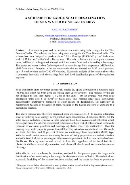
2overall objective rather than detailed design and cost calculations. Thus, an attempt has beenmade to present only the results of preliminary design and cost calculations.2. THAR DESERTThe northwest region of India is covered with a large desert known as the Thar Desert, whichoccupies an area of about 200,000 sq.m. [6]. Figure 1 shows the location of this desert andthe proposed site for the desalination unit. The desert is inhabited by about 3 million people,most of whom eke out a modest existence through subsistence agriculture [7]. The averageannual precipitation is about 150 mm, the monsoon months being from late July to earlySeptember; most of the deep wells are saline; and the water table is very low, in some placesas deep as 100-200 m. In some locales it has not rained for the past 80 yr [8]. There isalways the threat of famine in this area resulting in great loss of animal and human life.Nevertheless, through the ages local population has been able to identify and use some of thewild plants that grow in this area [9]. These plants grow with very little water availableduring the monsoon months, and it is hoped that if adequate water is available in this regionthen the quantity of such food together with other staple foods like Bajra can be greatlyincreased. Such optimism is also borne by the past history of the region, which indicates that,the confluence of man and nature has turned this rich area of flourishing Harrappian cultureinto desert [10].Several schemes for watering this area have been proposed, but most of them have proven tobe economically unfeasible. Among one of the schemes that is being actively pursued by theGovernment of India is the construction of a huge canal known as the Rajasthan Canal. Thiscanal, when completed, will be able to irrigate a substantial portion of the northern part of thedesert, but the scheme has been bogged down by rising cost of the canal and the lowering ofthe level of the Sutlej River, the source of this canal.

5and,m c p {T out (t) – T in (t)} = h 1 A i {T 1 (t) + T 2 (t) – T mm (t)} (4)T mm (t) = [T out (t) + T in (t)] /2.0 (5)It should be noted that steady state calculations have been made for the heat flow in thecollector from the top. There will be a thermal lag in the heat transfer to water because ofabsorption of heat by the pipe during the warm-up period in the morning. This heat gain willhave a tendency of being lost during the afternoon cooling-off period. However, the internalheat transfer coefficient h i inside the pipe is about 448 W/m 2 – 0 C as compared to externalheat transfer coefficient, h 0 of 33.6 W/m 2 – 0 C and thus most of the energy absorbed in thewalls of the pipe is transferred to the water.The base temperature T b (t) is calculated after knowing the soil surface temperature T s (t).Following the method outlined in [15] we find that the diurnal variations of the temperaturedies down after about 0.8 m below the surface and is a constant 12.7 0 C (55 0 F).Hence the sand surface temperature in the desert is given by the following equation for perunit area,α sand q'' (t) = h [T s (t)- T ∞ (t)] + (k sand /ΔX) [T s ( r) – 12.7] (6)Where ΔX = 0.8 m.Knowing q'' (t) and T ∞ (t) one can calculate T s (t) easily. There is a time lag between themaximum surface temperature and the maximum temperature 8.9 cm (3.5 in.) below thesurface and is given by [15],ξ = (l/2) [24/(ΠA)] 1/2 (7)Where l = depth below the surface and A = K s /(C p ρ) s . For the present case ξ is 3.7 hrs.Also the maximum temperature T b is given byT b, max = T s, amp exp {- l (Π/A) x 24] 1/2 }, (8)Where T s amp is the amplitude of the diurnal variation of soil surface temperature. For atypical day in June the top surface temperature, T s and T b are shown in Fig. 5. Table 2 liststhe property values used in the calculations above.Thus knowing the bottom temperature T b (t), eqns (1) - (5) have been solved to yield thetemperature of the outlet water from the solar collector. T out (t) from eqn (4) then becomesT in (t) for the next section of the collector, and thus the calculations proceed for the totallength of the collector. For a typical day in June the outlet temperature from the solarcollector is shown in Fig. 6. The inlet temperature to the solar field is a function of the outlet

6temperature. This relationship, shown in Fig. 7, can be calculated by making an enthalpybalance on the distillation unit [16]. In the above calculations it is assumed that the bottomof the collector temperature is the same as that of sand at depth of 8.9 cm, but which isexposed to solar radiation directly. In actual practice the bottom of the collector will becooler than the adjacent sand because of shading. However, heat loss calculations from thecollector to sand using temperature of 49 0 C (120 0 F) for a typical day in June at 2 p.m. yieldheat flow of about 480 W/m 2 . This heat loss is about 240 W/m 2 less than that from thecollector bottom, which is shaded. The above heat flow was estimated assuming the sametype of temperature profile of the sand parallel to collector, as that of the ground. Correctionsfor the above profile were made since the heat is conducted from both ends of the collector.The above heat loss translates into loss of distillate output of 10 per cent which is within theaccuracy of most heat transfer calculations. This then justifies the assumption of T b .Naturally, the above loss sets the upper limit on the heat flow to the sand and at other times itwill be much less and consequently the distillate loss will be much lower.

7The above set of calculations have been done for a typical day in January (the coldest month)and for March, and the outlet temperature-time history is shown in Fig. 6.Desalination unitThe heated seawater from the “solar field” goes to the desalination unit for production offresh water. The desalination unit is the regular multi-stage flash evaporation (MSF) type.Normally, these MSF units are used for brine temperatures of approximately 100 0 C (212 0 F)and thus would seem inappropriate at a first glance, for our scheme where the maximumbrine temperature is 60 0 C (140 0 F). Nevertheless, in the absence of any other viabledesalination technology we have used this system. We do, however, feel the need of betterand more efficient systems for evaporation of sea water, which would ultimately bring downthe cost of the scheme. It will be seen later than the MSF unit is one of the costliest item inthe whole scheme and thus the need of a better unit.The MSF unit for the present scheme is a 20-stage evaporator with terminal temperaturedifference (TTD) of 1.67 0 C (3 0 F). The present design is simply an extrapolation on the designby Brice et al. [5] for the production of about 1.36 x 10 3 m 4 /hr (3.6 MG/hr) of fresh water.Table 2 gives the various parameters of the unit. As can be expected the output from thedesalination unit depends upon the brine temperature entering in it. For different months theoutput of the unit has been calculated. The method for calculating the output is very wellknown [16] and those methods have been used in the present case.The distillate output starts as soon as the outlet temperature from the “solar field” reaches32.2 0 C (90 0 F). Thus for the month of June the scheme operates for 24 hr while for the monthof March it works for 19 hr and for the month of January only 9 hr.Figure 8 shows the output for various months. There is no output during the months of July,August and half of September since in these months the sky is mostly cloudy [7]. More overthese months can be used for yearly maintenance, if any. The integration of Fig. 8 than givesus the yearly output of 5.25 x 10 7 m 3 (13860MG) of fresh water.

8In most of the existing desalination plants with MSF units, scale build up is quite a majorproblem requiring large clean-up operations thereby shutting down the plant and use of costlychemicals for reducing it. The scale problem becomes more acute after temperatures if71.1 0 C (160 0 F) while below this temperature the severity of this problem is substantiallyreduced. Thus, in the present scheme since the maximum brine temperature is 60 0 C (140 0 F),the scale problem is minimized. This is one of the major advantages of operating at lowtemperatures.Pumping requirementsThe seawater has to be pumped from the Arabian Sea to the desalination site, which is 80 km(50 miles) from it and at an elevation of 45.7 m (150 ft) from the sea level. The pumps,hence, should be large enough to overcome the pressure loss in the feed pipes and theelevation. The feed pipes are three in number and are 3.05 m (10 ft) in diameter. They aremade of concrete and are 10.16 cm (4 in.) thick and will be buried in ground so as not to beheated. Table 3 shows the results of calculations for power required in this section of theplant.In addition to the above requirements, pumps are also needed to effect desalination. Thus inthe MSF unit, they should be able to overcome the pressure loss in heat exchangers as well asbe able to create enough suction for flash evaporation. For the pumping in the MSF plant wehave extrapolated on the design given by Brice et al. [5] to suit our requirements. Table 3shows the power required for MSF unit.

9The effluent from the MSF, it is proposed, will be allowed to flow by gravity back to theArabian Sea in a canal 11.9 m (39 ft) wide and 0.91 m (3 ft) deep, at a velocity of 6.4 km/hr(4 m.p.h.).The average wind velocity in this area is about 32 km/hr (20 m.p.h.) and sometimes goes ashigh as 28 km/hr (80 m.p.h.). Thus, it is quite logical to use wind turbines to pump the seawater. The wind turbines used in the present scheme are the 200 kW each capacity machineswhich are being actively experimented by the Department of Energy (DOE) for large scaledeployment in the 1980’s. The machines will be staggered throughout the length of the feedpipes and in the solar field. In the feed section they will be arranged in such a manner so thateach machine just overcomes the pressure loss and the elevation head equivalent to itscapacity. At the same time there will be one elevated storage tank attached to each machine,which will be filled up when the wind velocities go above 32 km/hr. Thus during the “windlean” periods the steady flow rate in the feed section will be maintained. The exact analysison the size of these tanks and their location has not been done since it is beyond the scope ofthis paper.Disposal of effluentsIn the present scheme, the rejected seawater is on an average about 2.03 x 10 5 m 3 (53.0 MG)per hr, and it is but natural to inquire if we cannot use this brine to extract salts like NaCl,KCl, and others. However, the effluents have a salt concentration of only 3.7 per cent, whichis still 96 per cent pure water and is not sufficiently shown to be, in general, an economicallyviable feed stock. Nevertheless, the decision on whether to extract the salts from this brinehave to be made, taking into consideration many local, national, and economic factors that itis again beyond the scope of the present paper.In such a large scale desalination plant study, it is also worthwhile to look at the effect ofeffluents on the marine environment. Very little work has been done on this aspect, but thestudies do indicate [10] that there is very little or negligible effect on the marine environment.Specifically, in our case, since we are operating at very low concentrations of salts and at thesame time, very near to the feed water temperature of 15.5 0 C (60 0 F), the harmful effects willbe negligible to the environment.4. COST ANALYSISIn any project of the magnitude and complexity like the present scheme, the calculations forthe cost of water can at best be an approximation. There are a multitude of local conditionsthat have to be taken into account for the final figures. In the absence of any such data, likethe cost of water in this region, cost of other alternatives and the payback mode for adesalination plant, it is appropriate that a simple minded cost calculation based on the capitaland running cost of the system should be sufficient. The capital cost includes the cost of windmachines, the cost of 20 stage MSF unit and the cost of concrete tubes. Also included in thecapital cost is the labor, which has been taken arbitrarily to be 20 per cent of the capital cost.The running cost includes the maintenance and the chemicals for scale reduction. Based onthe existing technology for such plants [12], the maintenance cost has been taken to be 7 percent of the capital cost.The cost of the wind machines is based upon the projected cost by DOE for the 1980’s [13]which is $2500 kW. For concrete collector tubes the existing market price of $12.50/ton has

10been taken. We do believe that large scale production of concrete locally will be muchcheaper than this price. The MSF desalination technology is quite developed and thus thecost of such plants has been extensively surveyed [12]. Based on such cost figures, thedesalination unit cost has been calculated. Brice et al. [5] have given detailed costs for aMSF desalination unit operating at 60 0 C (140 0 F) brine temperature. We have interpolated onthis design for condensing area requirements and cost for the present scheme. Table 4 givesthe various costs for the system. Assuming that present plant will provide water for 290 daysin a year, the cost of water per 3.79 m 3 (1000 gal.) is :Capital cost x (1.1) η -1 x 1000Cost of water $/3.79 m 3 ($/1000 gal.) = ------------------------------------ (9)13860 x ηwhere η = number of years.Figure 9 shows the cost of water with time. Naturally, this cost should be compared with thecost of water obtained from an alternative supply of water. The alternatives available in thisregion are (a) a canal from one of the rivers in North India and (b) another desalination plantrunning on fossil fuels. As for alternative (a), very little or no data is available and thus nomeaningful cost calculations can be done. Hence, we can only compare the cost of waterwith alternative (b) of the equivalent capacity. For such fuel fired MSF plants data isavailable [12]. Table 6 shows the various cost parameters involved in such a plant. The costof water for 3.79 m 3 (1000 gal.) is given by :where η = number of years.2.88Cost ($) = ---- x (1.1) ) η -1 + 4.74 (1.1) ) η -1 (10)η

11Figure 9 shows the comparison of the cost of water available from both the solar plant andfuel powered MSF plant. The point of intersection of the two curves is at about 8 yr, whichmeans that the water from the solar system becomes economically cheaper than that obtainedfrom the fossil fuel fired desalination plant after about 8 yr.Though the cost calculations done above are justified for the sake of completeness of thestudy there are other things, which sometimes are given priority, than cost, to make thescheme work. In an area where the level of poverty is unimaginable and where a smallamount of water together with the will and determination of these people will bring wondersto the land, it can be argued from the philosophical point of view that the water is priceless.Thus, a scheme of this nature and magnitude can only be funded by the government as a partof the social commitment to the people.5. CONCLUSIONSThe purpose of this study has been to look at technical and economical feasibility of a schemeto desalinate sea water using solar energy for Thar Desert in India. Based upon this study thefollowing conclusions can be drawn :1. An area of 11.52 km 2 (4.5 miles) of desert will be sufficient to produce 5.25 x 10 7 m 3(13860 MG) of fresh water every year.2. The pumping requirements for the whole scheme will be met by 415 wind machines eachof 200 kW capacity.3. The cost of water from the present scheme compares favorably with that from a fuel firedMSF plant, the crossover taking place at about 8 yr (Fig. 9).Finally, it is realized that the technological implications are staggering, but the impact on thenational economy, the welfare and employment of the local rural population and the effect onthe environment in terms of converting this desert into a great developmental area, appear tobe favorable and thus warrant further development and evaluation of the present scheme.Acknowledgement :- The author wishes to thank Dr. C. C. Oliver for his many helpfulsuggestions and critical comments.REFERENCES1. S. G. Talbert et al. Manual on Solar Distillation of Saline Water. Office of Saline Water,Research and Development Progress Report No. 546, Washington, D.C., U.S. Departmentof Interior (1970).2. E. D. Howe and B. W. Tleimat, Solar Distillation at the University of California. SolarEnergy 16, 97 (1974).3. K. S. Spiegler, Salt-Water Purification, p 84, Plenum Press, New York (1977).4. C. N. Hodges et al. Solar Distillation Utilizing Multiple-Effect Humidification. FinalRep., Solar Energy Laboratory of the Institute of Atmospheric Physics, University ofArizona (1966).

125. D. B. Brice, Saline Water Conversion by Flash Evaporation Utilizing Solar Energy. Adv.Chem. Ser 38, 99 (1963).6. Encyclopedia Britannica, Thar Desert, Encyclopedia Britannica Inc., London. Vol. 10, p.206 (1974).7. R. N. Kaul (editor) Indo-Pakistan. Afforestation in Arid Zones. Dr. W. Junk N. V.,Publishers. The Hague (1970).8. E. S. Hills, Research and the Future of Arid Lands, Methuen, London (1966).9. M. M. Bhandari, Famine foods in the Rajasthan Desert. Economic Botany 20 (1), 73(1974).10. P. K. Das, The Monsoons. St. Martin’s Press, New York (1968).11. R. S. Silver and W. S. McCartney, Desalination; The Marine Environment (Edited by J.Lenihan), Vol. 5. Academic Press, New York (1977).12. United Nations, Second United Nations Desalination Plant Operation Survey, U. N.Dept. of Economic and Social Affairs, New York (1973).13. A. B. Lovins, Soft Energy Paths, Ballinger, Cambridge, Massachusetts (1977).14. Monthly Labor Rev., Vol. 101, No. 2, U.S. Dept. of Labor, Bureau of Labor Statistics,Washington D.C. (Feb. 1978).15. E. R. G. Eckert and R. M. Drake, Jr., Analysis of Heat and Mass Transfer, McGraw-Hill,New York (1972).16. R. S. Silver, Distillation. In Principles of Desalination (Edited by K. S. Spiegler).Academic Press, New York (1966).

13Table 1. Heat transfer results for collector for a typical day in June at 2 p.m.Brine flow rateSolar radiationAbsorptivity of paintAverage ground temperature (8.9 cm. below the surface)Average ambient temperatureWind velocityOutside heat transfer coefficientInlet brine temperature (to the solar field)Outlet brine temperature (from the solar field)Residence time for the brine in solar field11.25 m 3 /hr (2970 gallons/hr)849 W/m 2 (294 BTU/ft 2 -hr)0.949 0 C (120 0 F)51.6 0 C (125 0 F)32 km/hr (20 mph)33.6 W/m 2 – 0 C (6 BTU/ft 2 –hr- 0 F)54.4 0 C (130 0 F)60 0 C (140 0 F)4 hrs.Table 2. Property values used in equations (1) to (8)α cbh c + rk ch ik sandα sandρ sandC p sand0.9 a33.6 W/m 2 – 0 C (6 BTU/ft 2 –hr- 0 F)1.82 W/m- 0 C (1.05 BTU/hr – ft – 0 F) a448.0 W/m 2 – 0 C (80 BTU/ft – hr - : F)0.347 W/m - 0 C (0.2 BTU/hr – ft 0 F) a0.82 a1518.5 kg/m 3 (94.8 1b/cu. ft.) a816 KJ/kg 0 C (0.195 BTU/1b 0 F) aa : Values taken from Standard Handbook for Mechanical Engineers Seventh Edition (1967).Table 3. Calculations for MSF unit (for a typical day in June)Area of condensing surfaceOutside diameter of the condensing tubeMaterial of the tubeNo. of stagesTerminal Temperature Difference (TTD)Total pump power required (to overcome pressure loss inheat exchanger and to create suction)Distillate producedMaximum temperature of sea water inTemperature of condensing waterTemperature of water going to solar fieldTemperature of blow down brineProduct water temperature1.41 x 10 6 m 2 (15.2 x 10 6 ft 2 )2.54 cm (1 inch)Cu/Ni Alloy201.67 0 C (3 0 F)4.47 x 10 4 kW (6 x 10 H.P.)1.36 x 10 4 m 3 /hr (3.6 MG/hr).60 0 C (140 0 F)15.5 0 C (60 0 F)54.4 0 C (130 0 F)26.6 0 C (80 0 F)25.5 0 C (78 0 F)

15NOMENCLATUREA 0 Outside area of the concrete collector, m 2 (ft 2 ).A 0 , A b Average areas of the top surface and bottom surface of the collector respectively,m 2 (ft 2 ).A Thermal diffusivity of sand k /A i Inside area of the collector, m 2 (ft 2 ).C ps , C p Specific heat of sand and water respectively, W s /kg k (Btu/lb.R).h c+r Outside heat transfer coefficient for convection and radiation, W/m 2 (Btu/ft 2 hr F).h i Inside heat transfer coefficient for water flowing in the collector, W/m 2 C (Btu/ft 2hrF).k c , k s Conductivity of concrete and sand respectively, W/m k (Btu/ft hr F).l Depth of ground below the surface eqn (7), m (ft).m Mass flow rate of sea water in the collector, kg/hr (lb/hr).q''(t) Incident solar insolation at time t, W/m 2 (Btu/ft hr).T b, max Maximum temperature of the ground 8.9 cm below the surface, 0 C ( 0 F).T s, amp Amplitude of the surface temperature in eqn (8), 0 C ( 0 F).T 1 , T 2, T 0, T b, T mm, T m T out , Temperatures shown in Fig. 4.T ∞, T s Temperatures of the ambient and surface of sand respectively 0 C ( 0 F).t c Thickness of the concrete collector, m (ft).ΔX Depth of the ground, eqn (6).α s Solar absorptivity of sand.α cb Solar absorptivity of blackened concrete.ξ Time lag between the maximum temperature of the surface of sand and that at 8.9cms below, hr.ρ s Density of sand, kg/m 3 (lb/ft 3 ).HOME