Structural Equation Models Estimation Maximum likelihood ...

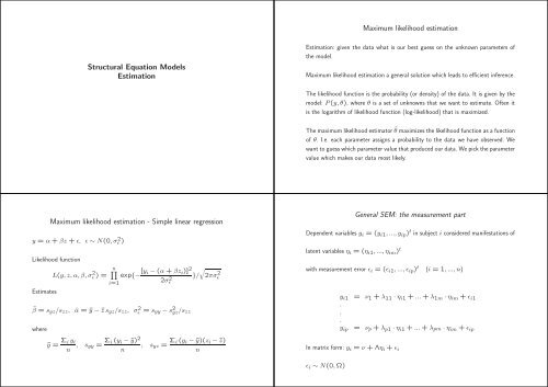
Maximum likelihood estimationStructural Equation ModelsEstimationEstimation: given the data what is our best guess on the unknown parameters ofthe model.Maximum likelihood estimation a general solution which leads to efficient inference.The likelihood function is the probability (or density) of the data. It is given by themodel: P (y, θ), where θ is a set of unknowns that we want to estimate. Often itis the logarithm of likelihood function (log-likelihood) that is maximized.The maximum likelihood estimator ̂θ maximizes the likelihood function as a functionof θ. I.e. each parameter assigns a probability to the data we have observed. Wewant to guess which parameter value that produced our data. We pick the parametervalue which makes our data most likely.Maximum likelihood estimation - Simple linear regressiony = α + βz + ǫ, ǫ ∼ N(0, σ 2 ǫ )Likelihood functionL(y, z, α, β, σǫ 2 n∏) = exp{− [y i − (α + βz i )] 2 √i=12σǫ2 }/ 2πσǫ2Estimateŝβ = s yz /s zz ,wherêα = ȳ − ¯z s yz /s zz , σ 2 ǫ = s yy − s 2 yz /s zzȳ = Σ i y in , s yy = Σ i (y i − ȳ) 2, s yz = Σ i (y i − ȳ)(z i − ¯z)nnGeneral SEM: the measurement partDependent variables y i = (y i1 , ..., y ip ) t in subject i considered manifestations oflatent variables η i = (η i1 , ..., η im ) twith measurement error ǫ i = (ǫ i1 , ..., ǫ ip ) t (i = 1, ..., n)y i1 = ν 1 + λ 11 · η i1 + ... + λ 1m · η im + ǫ i1...y ip = ν p + λ p1 · η i1 + ... + λ pm · η im + ǫ ipIn matrix form: y i = ν + Λη i + ǫ iǫ i ∼ N(0, Ω)

General SEM: the structural partLinear relations between latent variables η i = (η i1 , ..., η im ) tand independent variables z i = (z i1 , ..., z iq ) twith residuals ζ i = (ζ i1 , ..., ζ im ) tDistribution of observed variablesStructural part: η i = α + Bη i + Γz i + ζ igives: η i = (I − B) −1 α + (I − B) −1 Γz i + (I − B) −1 ζ iη i1 = α 1 + Σ j≠1 β 1j η ij + Σ j γ 1j z ij + ζ i1...η im = α m + Σ j≠m β mj η ij + Σ j γ mj z ij + ζ imMeasurement part: y i = ν + Λη i + ǫ igives: y i = ν + Λ(I − B) −1 α + Λ(I − B) −1 Γz i + Λ(I − B) −1 ζ i + ǫ iDistribution of y i given z i is multivariate regression model.In matrix form: η i = α + Bη i + Γz i + ζ iζ i ∼ N(0, Ψ)Estimationy i |z i ∼ N p {µ(θ) + Π(θ)z i , Σ(θ)}, with θ=(ν, Λ, Ω, α, B, Γ, Ψ)• µ(θ) = ν + Λ(I − B) −1 α• Π(θ) = Λ(I − B) −1 Γ• Σ(θ) = Λ(I − B) −1 Ψ(I − B) −1t Λ t + ΩL(y, z, θ) =n∏exp{−[y i − µ(θ) − Π(θ)z i ] t Σ(θ) −1 [y i − µ(θ) − Π(θ)z i ]/2}/ √ |Σ(θ)|i=1ML estimator maximizes L(y, z, θ) as a function of θ.This is multivariate regression model complicated by the fact that parameters appearin a non-linear way (e.g., products, and inverse).General SEM: Normality assumption for independent variablesy|z ∼ N p {µ(θ) + Π(θ)z, Σ(θ)}, θ=(ν, Λ, Ω, α, B, Γ, Ψ)Assume z ∼ N(µ z , Σ z ), then v = (y, z) has normal distributionE Θ (v) =Θ = (θ, µ z , Σ z )( )ν(θ) + Π(θ)µz, varµ Θ (v) =z( )Π(θ)Σz Π(θ) t + Σ(θ) .Σ z Π(θ) t Σ zThe SEM model induces a specific structure on the mean and variance in the multivariatenormal distribution.If the number of subjects is high there are many factors in the likelihood function.

The log-likelihood functionlog L(y, z, Θ) = log[ ∏ ni=1 exp{−[v i − E Θ (v)] t var Θ (v) −1 [v i − E Θ (v)]/2}/ √ |var Θ (v) −1 |]= − log |var Θ (v)| − tr[S var Θ (v) −1 ] − [¯v − E Θ (v)] t var Θ (v) −1 [¯v − E Θ (v)]Note that the likelihood function depends on the data only through the empiricalmean and covariance.The empirical mean and covariancev i = (y t i , zt i )t - column of both dependent and independent variables⎛ ⎞ ⎛⎞¯v 1s 11 . . s 1(p+q)⎜ . ⎟ ⎜ . . . . ⎟¯v = ⎝.⎠ S = ⎝. . . .⎠¯v (p+q) s (p+q)1 . . s (p+q)(p+q)¯v j = Σ i v ijnv jk = Σ i (v ij − ¯v .j )(v ik − ¯v .k )(n − 1)Empirical mean and covariance are sufficientEstimation process explainedLikelihood function depends on the data only through ¯v, S. Two data sets with thesame empirical mean and covariance will yield the same estimates.1. For each value of the model parameters (Θ) calculate the theoretical meanand covariance.Structural equation models use only the information in the mean and covariance.In many SEM packages, instead of data sets of single observations, you can runthe analysis based only on the mean and covariance. We do not recommend thisapproach - you lose some possibilities to test the model.2. Calculate how close the theoretical mean and covariance is to the observedmean and covariance.3. Find the value of Θ where the theoretical mean and covariance is closest tothe observed values.

Illustration of estimation processSimple linear regression viewed as a bivariate normal modelA very simple SEM is the standard regression model:× datay = α + βz + ǫ, ǫ ∼ N(0, σ 2 ǫ ) - z is usually considered fixedmodelEach point on the curve corresponds to a mean and covariance matrix in the model. The observedmean and covariance matrix is the cross. When we estimate the parameters we find the meanand covariance matrix in our which minimizes the distance to the data.Assume z ∼ N(µ, σz 2 ). Then (y, z) bivariate normal:( )yEz=(α + βµµ) ( )y, varzThis is a model in the bivariate normal distribution.=( )β 2 σz 2 + σǫ 2 .βσz 2 σ 2Sometimes the model is so high dimensional that the it can describe the observed covariancematrix perfectly (zero degrees of freedom).Estimation in the bivariate modelIn this example the parameters can be chosen such that the theoretical covariancebecomes equal to the observed covariance:Normal distribution for covariates?Maximum likelihood inference in the model where z is assumed be normally distributedand our SEM model conditioning on z is equivalent.(α + βµµ)=( )ȳ,¯z(β 2 σ 2 z + σ 2 ǫ βσ 2 zβσ 2 zσ 2 z)=( )syy s yzs yz s zzGeneral result: p(y, z) = p(y|z)p(z)Log-likelihood function is a sumσ 2 z = s zz, βσ 2 z = s yz ⇒ β = s yz /s zzβ 2 σ 2 z + σ 2 ǫ = s yy ⇒ σ 2 ǫ = s yy − s 2 y,z/s zzlog[L(y, z|θ, µ z , Σ z )] = log[L(y|z, θ)] + log[L(z|µ z , Σ z )]µ = ¯z, α + βµ = ȳ ⇒ α = ȳ − ¯z s yz /s zzNote that we obtain exactly the same estimates for α, β and σ 2 ǫwhich do not assume a normal distribution for the covariate.as in the standard regressionThe log-likelihood in the multivariate model where the covariate is normal is equalto the log-likelihood our SEM plus the log-likelihood of the model for the covariate.Whether we maximize the sum or only the first term in θ we get the same.

Thinking about SEMsStructural Equation Modelsχ 2 -test of model fitYou can think about a SEM as being a model in the multivariate normal distribution.If you have 5 dependent and 5 independent variables then your model consists of 10-dimensional normal distributions. These distributions are given uniquely by the meanand the covariance matrix. So you model includes means and covariance matrices.The saturated model includes all 10 dimensional mean vectors and all 10-dimensionalcovariance matrices. Your model includes only some of these.Hypothesis testingAssume that we have a SEM with and we want to test that some parameters arezero, e.g., no mercury effect. Then the strongest test is the likelihood ratio test.Testing the hypothesis H 0 : β = 0. You then maximize the log-likelihood in yourmodel [log(L)] and under H 0 [log(L H0 )]. Then you calculate the difference inminus to times the log-likelihoods−2[log(L H0 ) − log(L)]A general test of goodness of fitHow can I test if may model fits well?You can compare to a larger model in a likelihood ratio test?OK, what model should I use for comparison.General solution: the saturated model.The p-value is then calculated in the χ 2 -distribution with degrees of freedom equalto the parameters your are testing.

Joint model - Part of the output--------------------------------------------------Number of observations = 712Log-Likelihood = -20072.96BIC = 41401.15AIC = 40425.91log-Likelihood of model = -20072.96log-Likelihood of saturated model = -18586.80Chi-squared statistic: q = 2972.317 , df = 69 , P(Q>q) = 0--------------------------------------------------Model search using modification indicesIn SEM literature often denoted modification indices MIMI s measure how much better the model-fit would become if each fixed parameter was set freeto be estimated.If θ fixed: θ = θ 0 , MI tests the hypothesis H 0 : θ = θ 0 against H a : θ ≠ θ 0 .Under H 0 : MI ∼ χ 2 1 .Chi-squared statistic tests your model against the saturated model.The log-likelihoods are:log-Likelihood of model = -20072.96log-Likelihood of saturated model = -18586.80If MI is high, then it is a sign that the corresponding model restriction is not supported by thedata (see also Bollen pp 299-302).MI s in lava: to get 10 most important extensionsprint(ms q) = 0This model is rejected. The degrees of freedom is 69. It means that if you added 69 associations tothe path diagram then you would have the saturated model. So some of these missing associationsare important, but the test cannot tell you which.Score: S P(S>s) Index holm BH75.89 0 dsbnt1 0 0123.9 0 ft1ft3 0 0138 0 cvlt1cvlt3 0 0141.4 0 bnt1cvlt1 0 0147.4 0 bnt2cvlt1 0 0166.2 0 ft2ft3 0 0182.9 0 cvlt1cvlt2 0 0189.8 0 cvlt2cvlt3 0 0294.7 0 ft1ft2 0 0624.4 0 bnt1bnt2 0 0Output from ’summary(m3)’The most important modification is to allow for a correlation between the twooutcomes bnt1 and bnt2. This modification is highly significant also after adjustmentfor multiple testing (columns: holm, BH).Note: if you make one modification then the other MIs may change - because we anow looking a modifications to another model.