Stat Crunch - Napa Valley College

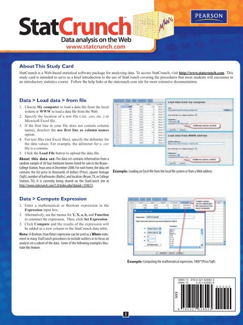
Graphics > QQ Plot1. Select the column(s) to be displayed.2. Use an optional Where statement to specify the data included.3. Select an optional Group by column to produceseparate plots for different groups.4. Click Create Graph! to construct the plot(s).Interacting with Graphics1. Click and drag the mouse around graph objects tohighlight them.2. The corresponding rows will be highlighted in thedata table and in all other graphics.3. Toggle highlighting on and off by clicking on the rownumber in the data table.4. To clear all highlighted rows, click on the Row headingatop the first column in the data table.5. To highlight rows based on categories or numericranges, use the Data > Row selection > Interactivetools option.Stat > Summary Stats > Columns1. Select the column(s) for which summary statistics areto be computed.2. Use an optional Where statement to specify the dataincluded.3. Compare statistics across groups using an optionalGroup by column.4. Click Next for additional options such as the statisticsto be computed.5. Click Calculate to compute the summary statistics.Example: QQ plot of the Sqft column grouped by LocationExample: Highlighting an outlier in a boxplotStat > Tables > Frequency1. Select the column(s) for which a frequency table is tobe computed.2. Use an optional Where statement to specify the dataincluded.3. Click Calculate to compute the frequency table(s).Example: Comparing prices of homes listed in Bryan to those listed in CollegeStation with the potential outlier removed3Example: A frequency table for the number of bathrooms

Stat > Proportions > One sample1. Choose the with data option to use data from the datatable.a. Select the column containing the sample values.b. Specify the outcome that denotes a success.c. Use an optional Where statement to specify the dataincluded.Choose the with summary option to enter the number ofsuccesses and number of observations.2. Click Next and select the hypothesis test or confidenceinterval option.a. For a hypothesis test, enter the Null proportion andchoose Z, 6 , or 7 for Alternative.b. For a confidence interval, enter a value between 0 and 1for Level (0.95 provides a 95% confidence interval).For Method, choose Standard-Wald or Agresti-Coull.3. Click Calculate to view the results.Stat > Proportions > Two sample1. Choose the with data option to use sample data from theStatCrunch data table.a. Select the columns containing the first and second samples.b. Specify the sample outcomes that denote a success forboth samples.c. Enter optional Where statements to specify the data rowsto be included in both samples. If the two samples are inseparate columns, this step is typically not required.Choose the with summary option to enter the number ofsuccesses and number of observations for both samples.2. Click Next and select the hypothesis test or confidenceinterval option.a. For a hypothesis test, enter the Null proportion differenceand choose Z, 6 , or 7 for Alternative.b. For a confidence interval, enter a value between 0 and 1for Level (0.95 provides a 95% confidence interval).3. Click Calculate to view the results.Example: For each of 998 North Carolina births, this data set indicates whetheror not the birth was premature. A 95% confidence interval for the proportion of allNorth Carolina births that are not premature is shown above.Example: In a survey,181 of 336 people who attended church services at least oncea week said the use of torture against suspected terrorists is “often” or “sometimes”justified. Only 71 of 168 people who “seldom or never” went to services agreed. Usingthis summary information, a two-sided hypothesis test is performed below to comparethe proportion with this opinion for these two populations.Stat > T statistics > One sample1. Choose the with data option to use sample data from theStatCrunch data table.a. Select the column containing the sample data values.b. Use an optional Where statement to specify the dataincluded.Choose the with summary option to enter the samplemean, sample standard deviation, and sample size.2. Click Next and select the hypothesis test or confidenceinterval option.a. For a hypothesis test, enter the Null mean and chooseZ, 6 , or 7 for Alternative.b. For a confidence interval, enter a value between 0 and1 for Level (0.95 provides a 95% confidence interval).3. Click Calculate to view the results.Example: Testing to see if the average home listed in College Station,Texas, is largerthan 2000 square feet.4

Stat > T statistics > Two sample1. Choose the with data option to use sample data from thedata table.a. Select the columns containing the first and second samples.b. Enter optional Where statements to specify the data rows tobe included in both samples. If the two samples are in separatecolumns, this step is typically not required.Choose the with summary option to enter the sample mean,sample standard deviation, and sample size for both samples.2. Deselect the Pool variance option if desired.3. Click Next and select the hypothesis test or confidenceinterval option.a. For a hypothesis test, enter the Null mean difference andchoose Z, 6 , or 7 for Alternative.b. For a confidence interval, enter a value between 0 and 1 forLevel (0.95 provides a 95% confidence interval).4. Click Calculate to view the results.Example: Hypothesis test comparing the prices of homes listed in Bryan to thosein College Station, with potential outliers included.Stat > T statistics > Paired1. Select the columns containing the first and second samples.2. Use an optional Where statement to specify the data included.3. Click Next and select the hypothesis test or confidenceinterval option.a. For a hypothesis test, enter the Null mean difference andchoose Z, 6 , or 7 for Alternative.b. For a confidence interval, enter a value between 0 and 1 forLevel (0.95 provides a 95% confidence interval).4. Click Calculate to view the results.Stat > Regression > Simple LinearExample: A 95% confidence interval for the average difference between thegraduation rate of full- and part-time students across all colleges based on a randomsample of four colleges.1. Select the X variable (independent variable) and Y variable (dependent variable) for the regression.2. Use an optional Where statement to specify the data included.3. Compare results across groups by selecting an optional Group by column.4. Click Next to specify optional X values for predictions and to indicate whether or not to save residuals/fitted values.5. Click Next again to choose from a list of optional graphics for plotting the fitted line and examining residuals.6. Click Calculate to view the results.5Example: Regression of Price on Sqft for College Station

Stat > ANOVA > One way1. Select one of the following options:a. If the samples are in separate columns, select the Compareselected columns option and then select the columns containingthe samples.b. If the samples are in a single column, select the Comparevalues in a single column option. Then specify the columncontaining the samples (Responses In) and the column containingthe population labels (Factors In).2. Use an optional Where statement to specify the data to beincluded.3. Select the Tukey HSD option and specify a confidence level toperform a post hoc means analysis. The default value of 0.95provides 95% confidence intervals for all pairwise mean differences.4. Click Calculate to view the results.Example: ANOVA for the time, in minutes, a caller stays on hold before hangingup under three different treatments.Stat > Tables > Contingency1. Select one of the following options:a. Choose the with data option to cross tabulate two columnsof raw data from the data table. Then,A. Select the column to be tabulated across the rows.B. Select the column to be tabulated across the columns.C. Use an optional Where statement to specify the data included.D. Select an optional Group by column to compute separatetables across groups.b. Choose the with summary option to use a two-way crossclassification already entered in the data table. Then,A. Select the columns that contain the summary counts.B. Select the column that contains the row labels.C. Enter a name for the column variable.2. Click Next to specify additional information to be displayed ineach table cell.3. Click Calculate to view the results.Stat > Calculators1. Select the name of the desired distributionfrom the menu listing(e.g., Binomial, Normal, etc.).2. In the first line below the plot in thecalculator window, specify the distributionparameters. As examples, withthe normal distribution, specify themean and standard deviation or withthe binomial distribution, specify nand p.3. In the second line below the plot,Example: Finding a binomialspecify the direction of the desiredprobabilityprobability.a. To compute a probability, enter a value to the right of the directionselector and leave the remaining field empty(e.g., P(X 6 3 ) = ___ ).Example: Using summary counts cross tabulating gender and back problems, atest of independence between the two factors is shown below. Note that the backproblems variable is represented by the second and third columns in the data table.Example: Finding a standardnormal probabilityExample: Finding a t(8) quantileb. To determine the point that will provide a specified probability, enter the probability to the right of the direction selector and leave theother field empty (e.g., P(X 7 ) = 0.25). This option is available only for continuous distributions.4. Click Compute to fill in the empty fields and to update the graph of the distribution.6