identification of animal spirits in a bounded rationality model: an ...
identification of animal spirits in a bounded rationality model: an ...
identification of animal spirits in a bounded rationality model: an ...

You also want an ePaper? Increase the reach of your titles
YUMPU automatically turns print PDFs into web optimized ePapers that Google loves.
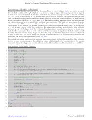
No 2012-12<strong>identification</strong> <strong>of</strong> <strong><strong>an</strong>imal</strong> <strong>spirits</strong><strong>in</strong> a <strong>bounded</strong> <strong>rationality</strong> <strong>model</strong>:<strong>an</strong> application to the euro areaby Tae-Seok J<strong>an</strong>g <strong>an</strong>d Stephen Sachtissn 2193-2476
Identification <strong>of</strong> Animal Spirits <strong>in</strong> a BoundedRationality Model: An Application to the Euro AreaTae-Seok J<strong>an</strong>g ∗ <strong>an</strong>d Stephen Sacht §October 10, 2012AbstractIn this paper we empirically exam<strong>in</strong>e a heterogenous <strong>bounded</strong> <strong>rationality</strong>version <strong>of</strong> a hybrid New-Keynesi<strong>an</strong> <strong>model</strong>. The <strong>model</strong> is estimated viathe simulated method <strong>of</strong> moments us<strong>in</strong>g Euro Area data from 1975Q1to 2009Q4. It is generally assumed that agents’ beliefs display waves <strong>of</strong>optimism <strong>an</strong>d pessimism - so called <strong><strong>an</strong>imal</strong> <strong>spirits</strong> - on future movements<strong>of</strong> the output <strong>an</strong>d <strong>in</strong>flation gap. Our ma<strong>in</strong> empirical f<strong>in</strong>d<strong>in</strong>gs show that a<strong>bounded</strong> <strong>rationality</strong> <strong>model</strong> with cognitive limitation provides a reasonablefit to auto- <strong>an</strong>d cross-covari<strong>an</strong>ces <strong>of</strong> the data. This result is ma<strong>in</strong>ly drivenby a high degree <strong>of</strong> <strong>in</strong>tr<strong>in</strong>sic persistence <strong>in</strong> the output <strong>an</strong>d <strong>in</strong>flation gap dueto the impact <strong>of</strong> <strong><strong>an</strong>imal</strong> <strong>spirits</strong> on economic dynamics. Further, over thewhole time <strong>in</strong>terval the agents had expected moderate deviations <strong>of</strong> thefuture output gap from its steady state value with low uncerta<strong>in</strong>ty. F<strong>in</strong>ally,we f<strong>in</strong>d strong evidence for <strong>an</strong> autoregressive expectation formation processregard<strong>in</strong>g the <strong>in</strong>flation gap.Keywords: Animal Spirits; Bounded Rationality; Discrete Choice Theory;Euro Area; New-Keynesi<strong>an</strong> Model; Simulated Method <strong>of</strong> Moments.JEL classification: C53, D83, E12, E32.∗ Department <strong>of</strong> Economics, Christi<strong>an</strong>-Albrechts-University Kiel, Olshausenstrasse 40,24118 Kiel, Germ<strong>an</strong>y. Email: taeseok.j<strong>an</strong>g@gmail.com§ Kiel Institute for the World Economy, H<strong>in</strong>denburgufer 66, 24105 Kiel & Department <strong>of</strong>Economics, Christi<strong>an</strong>-Albrechts-University Kiel, Olshausenstrasse 40, 24118 Kiel, Germ<strong>an</strong>y.Email: sacht@economics.uni-kiel.deWe th<strong>an</strong>k Paul De Grauwe, Marcel Förster, Re<strong>in</strong>er Fr<strong>an</strong>ke <strong>an</strong>d Thomas Lux for valuablediscussions <strong>an</strong>d suggestions. Furthermore we greatly acknowledge the particip<strong>an</strong>ts<strong>of</strong> the 2011 Macroeconometric Workshop at the DIW Berl<strong>in</strong>, the 17th Spr<strong>in</strong>g Meet<strong>in</strong>g <strong>of</strong>Young Economists at the ZEW M<strong>an</strong>nheim <strong>an</strong>d the 2012 Annual Meet<strong>in</strong>g <strong>of</strong> the Germ<strong>an</strong>Economic Association at the University <strong>of</strong> Gött<strong>in</strong>gen for helpful comments. This researchreceived generous support from the Graduate Student Best Paper Prize 2012 <strong>of</strong> the Society<strong>of</strong> Computational Economics awarded at the 18th International Conference Comput<strong>in</strong>g <strong>in</strong>Economics <strong>an</strong>d F<strong>in</strong><strong>an</strong>ce <strong>in</strong> Prague.1
1 IntroductionRational expectations are a flexible <strong>an</strong>d natural way <strong>of</strong> <strong>model</strong><strong>in</strong>g market behavior<strong>in</strong> dynamic stochastic general equilibrium (DSGE) <strong>model</strong>s, which arewidely used by macroeconomists. S<strong>in</strong>ce the DSGE approach disposes a convenient<strong>an</strong>alytical tractability under the assumption <strong>of</strong> rational expectations, this<strong>model</strong><strong>in</strong>g framework serves as <strong>an</strong> efficient toolbox for <strong>an</strong>alyz<strong>in</strong>g monetary <strong>an</strong>dfiscal policy measures. As Selten (2001) states, however, "modern ma<strong>in</strong>streameconomic theory is largely based on <strong>an</strong> unrealistic picture <strong>of</strong> hum<strong>an</strong> decisiontheory" s<strong>in</strong>ce evidence from experimental studies supports <strong>in</strong>formation process<strong>in</strong>gwith limited cognitive ability <strong>of</strong> agents rather th<strong>an</strong> perfect <strong>in</strong>formation (seeHommes (2011) among others). Indeed, a plethora <strong>of</strong> studies have been done onalternative forms <strong>of</strong> <strong>in</strong>formation process<strong>in</strong>g mech<strong>an</strong>isms <strong>in</strong> macroeconomics; seee.g. the literature on learn<strong>in</strong>g (Ev<strong>an</strong>s <strong>an</strong>d Honkaphohja (2001)), rational <strong>in</strong>attention(Sims (2003)), sticky <strong>in</strong>formation (M<strong>an</strong>kiw <strong>an</strong>d Reis (2002)) or <strong>bounded</strong><strong>rationality</strong> <strong>in</strong> general (Sargent (1994) <strong>an</strong>d Kahnem<strong>an</strong> (2003)). Camerer (1998)also <strong>of</strong>fers <strong>an</strong> <strong>in</strong>formative overview <strong>of</strong> the discussion on this topic <strong>in</strong> economics.For the most part <strong>of</strong> the behavioral research, we c<strong>an</strong> treat the realization <strong>of</strong>economic decisions as be<strong>in</strong>g a complex <strong>an</strong>d <strong>in</strong>teractive process between differenttypes <strong>of</strong> agents. Keynes (1936) already attributed signific<strong>an</strong>t ir<strong>rationality</strong> tohum<strong>an</strong> nature <strong>an</strong>d discussed the impacts <strong>of</strong> waves <strong>of</strong> optimism <strong>an</strong>d pessimism- so called <strong><strong>an</strong>imal</strong> <strong>spirits</strong> - on economic outcome. Accord<strong>in</strong>g to Akerl<strong>of</strong> <strong>an</strong>dShiller (2009), the emotional states are reflected <strong>in</strong> economic behavior - see alsoFr<strong>an</strong>ke (forthcom<strong>in</strong>g) for his extensive discussion about market behavior <strong>an</strong>dhow expectation formation should be treated <strong>in</strong> macroeconomic <strong>model</strong>s.In this paper we attempt to empirically exam<strong>in</strong>e the hypothesis that thebehavioral heterogeneity will have a macroscopic impact on the economy. Thepo<strong>in</strong>t <strong>of</strong> view taken here is that a behavioral <strong>model</strong> c<strong>an</strong> provide a conceptualframework for a cognitive ability as well as a subst<strong>an</strong>tial degree <strong>of</strong> <strong>in</strong>ertia <strong>in</strong>the DSGE <strong>model</strong>s. Accord<strong>in</strong>g to De Grauwe (2011), if agents are known to beeither optimists or pessimists, their ability (or better: limitation) to form theirexpectations affects economic conditions, i.e. movements <strong>in</strong> employment, theoutput gap <strong>an</strong>d <strong>in</strong>flation, more appropriately th<strong>an</strong> st<strong>an</strong>dard rational expectation<strong>model</strong>s. Indeed, it is shown <strong>in</strong> the expectation formation process under<strong>bounded</strong> <strong>rationality</strong> that we c<strong>an</strong> explicitly <strong>model</strong> <strong><strong>an</strong>imal</strong> <strong>spirits</strong> by apply<strong>in</strong>gdiscrete choice theory on group behavior. Then the behavior <strong>of</strong> optimists <strong>an</strong>dpessimists is considered to be a by-product <strong>of</strong> the switch<strong>in</strong>g mech<strong>an</strong>isms basedon the perform<strong>an</strong>ce measure from agents’ expectations (see also e.g. Westerh<strong>of</strong>f(2008) as well as Lengnick <strong>an</strong>d Wohltm<strong>an</strong>n (forthcom<strong>in</strong>g) among others).To the best <strong>of</strong> our knowledge, however, <strong>an</strong> empirical evaluation <strong>of</strong> a <strong>bounded</strong><strong>rationality</strong> <strong>model</strong> <strong>of</strong> this type discussed above is miss<strong>in</strong>g <strong>in</strong> the literature so far.We fill the exist<strong>in</strong>g gap between the use <strong>of</strong> the <strong>model</strong>s <strong>an</strong>d their empiricalevaluations <strong>in</strong> the literature by measur<strong>in</strong>g the effects <strong>of</strong> psychological behavioron the economy under consideration <strong>of</strong> <strong><strong>an</strong>imal</strong> <strong>spirits</strong>. We show that themoment-based estimation (Fr<strong>an</strong>ke et al. (2011)) c<strong>an</strong> be easily used to estimatea small-scale DSGE <strong>model</strong>. Ma<strong>in</strong>ly, similarities <strong>an</strong>d dissimilarities betweentwo polar cases <strong>of</strong> expectation formation processes will be exam<strong>in</strong>ed: while2
the underly<strong>in</strong>g <strong>model</strong> structure is identical to a st<strong>an</strong>dard three-equations New-Keynesi<strong>an</strong> <strong>model</strong> (NKM), we also allow both for rational expectations <strong>an</strong>dfor endogenously-formed expectations us<strong>in</strong>g the behavioral specification by DeGrauwe (2011). In particular, we study his behavioral economic framework <strong>an</strong>dprovide <strong>an</strong> empirical <strong>in</strong>vestigation <strong>of</strong> <strong>bounded</strong> <strong>rationality</strong> on economic dynamics<strong>in</strong> the Euro Area from 1975Q1 to 2009Q4. Accord<strong>in</strong>gly, <strong>an</strong> import<strong>an</strong>t aspect <strong>of</strong>this paper is to test the <strong>bounded</strong> <strong>rationality</strong> hypothesis <strong>in</strong> order to <strong>of</strong>fer reliableparameter values that c<strong>an</strong> be used for calibration <strong>in</strong> more realistic-grounded futurework, e.g. study<strong>in</strong>g monetary <strong>an</strong>d fiscal policy <strong>an</strong>alysis <strong>in</strong> a DSGE <strong>model</strong>without the assumption <strong>of</strong> rational expectations.In our empirical application, we show that the NKM with rational expectationsor <strong>bounded</strong> <strong>rationality</strong> c<strong>an</strong> generate auto- <strong>an</strong>d cross-covari<strong>an</strong>ces <strong>of</strong> theoutput gap, the <strong>in</strong>flation gap <strong>an</strong>d the <strong>in</strong>terest gap, which c<strong>an</strong> mimic real datawell. A quadratic objective function is used <strong>in</strong> the estimation to measure thedist<strong>an</strong>ce between the <strong>model</strong>-generated <strong>an</strong>d empirical moments. As the usualprocedure <strong>of</strong> the method <strong>of</strong> moments, the global m<strong>in</strong>imum <strong>of</strong> the objective functionprovides consistent parameter estimates <strong>of</strong> the <strong>model</strong>. Then we evaluatethe goodness-<strong>of</strong>-fit <strong>of</strong> the <strong>model</strong> to the data from the value <strong>of</strong> the quadratic objectfunction; i.e. the lower this value, the better the fit <strong>of</strong> the <strong>model</strong>-generatedmoments to their empirical counterparts. The empirical application us<strong>in</strong>g themethod <strong>of</strong> moment approach stays <strong>in</strong> l<strong>in</strong>e with the work <strong>of</strong> Fr<strong>an</strong>ke et al. (2011),who estimate a similar version <strong>of</strong> the NKM presented here for two sub-samples,i.e. the Great Inflation <strong>an</strong>d Great Moderation period <strong>in</strong> the US. They come tothe conclusion that <strong>in</strong>flation dynamics are primarily driven by <strong>in</strong>tr<strong>in</strong>sic ratherth<strong>an</strong> extr<strong>in</strong>sic persistence - which is the total opposite <strong>of</strong> the results when apply<strong>in</strong>gBayesi<strong>an</strong> estimation. This is reflected by a high degree <strong>of</strong> price <strong>in</strong>dexation<strong>an</strong>d a low degree <strong>of</strong> persistence <strong>in</strong> the assumed AR(1) cost-push shock. Ingeneral, this k<strong>in</strong>d <strong>of</strong> estimation technique is closely related to the approaches<strong>of</strong> <strong>in</strong>direct <strong>in</strong>ference with the difference that <strong>in</strong> our case the structural form <strong>of</strong>a DSGE <strong>model</strong> is used <strong>in</strong>stead <strong>of</strong> <strong>an</strong> auxiliary <strong>model</strong> like a SVAR (cf. Smith(1993) <strong>an</strong>d Christi<strong>an</strong>o et al. (2005) among others).Ma<strong>in</strong> f<strong>in</strong>d<strong>in</strong>gs c<strong>an</strong> be summarized as follows. First, over the whole time<strong>in</strong>terval the agents had expected moderate deviations <strong>of</strong> the future output gapfrom its steady state value with low uncerta<strong>in</strong>ty. Second, we f<strong>in</strong>d strong evidencefor <strong>an</strong> autoregressive expectation formation process regard<strong>in</strong>g the <strong>in</strong>flation gap,which is <strong>in</strong> l<strong>in</strong>e with the scientific consensus among experimental economists(Roos <strong>an</strong>d Schmidt (2012)).The rema<strong>in</strong>der <strong>of</strong> the paper is structured as follows. Section 2 <strong>in</strong>troduces asmall-scale NKM <strong>an</strong>d discusses two <strong>model</strong> specifications, i.e. one with rationalexpectations <strong>an</strong>d the other under consideration <strong>of</strong> the <strong><strong>an</strong>imal</strong> <strong>spirits</strong>. The estimationmethodology is presented <strong>in</strong> section 3. Section 4 then estimates twoversions <strong>of</strong> the <strong>model</strong> by the moment-based estimation <strong>an</strong>d discusses their empiricalresults. Afterwards, the properties <strong>of</strong> the moment-based procedure forestimation are exam<strong>in</strong>ed through a Monte Carlo study <strong>an</strong>d a sensitivity <strong>an</strong>alysis<strong>in</strong> section 5. F<strong>in</strong>ally, section 6 concludes. The appendix collects all relev<strong>an</strong>ttechnical details.3
<strong>an</strong>d Ropele (2009) observe that the dynamic properties (i.e. ma<strong>in</strong>ly the stability<strong>of</strong> the system) depend on the variation <strong>in</strong> trend <strong>in</strong>flation. Cogley <strong>an</strong>dSbordone (2008) also provide evidence for the expl<strong>an</strong>ation <strong>of</strong> <strong>in</strong>flation persistenceby consider<strong>in</strong>g a time-vary<strong>in</strong>g trend <strong>in</strong> <strong>in</strong>flation. In the same ve<strong>in</strong>, we c<strong>an</strong>ab<strong>an</strong>don the assumption <strong>of</strong> a const<strong>an</strong>t natural rate <strong>of</strong> <strong>in</strong>terest as be<strong>in</strong>g empiricallyunrealistic. In this paper, we follow the empirical approaches proposedby Cogley et al. (2010), Castelnuovo (2010), Fr<strong>an</strong>ke et al. (2011) among others,who also consider gap specifications for <strong>in</strong>flation (<strong>an</strong>d the nom<strong>in</strong>al <strong>in</strong>terestrate). Furthermore, <strong>in</strong>flation <strong>an</strong>d money growth are likely to be non-stationary<strong>in</strong> the Euro Area data. If that is the case, the estimation methodology such asthe method <strong>of</strong> moments approach presented here (or the generalized method <strong>of</strong>moments <strong>in</strong> general) will lead to biased estimates. 1 Taken this <strong>in</strong>to account, <strong>in</strong>the current study we consider the gaps rather th<strong>an</strong> the levels <strong>in</strong> order to ensurethe stationary <strong>of</strong> the times series.To make the description <strong>of</strong> the expectation formation processes more explicit,first we exam<strong>in</strong>e two polar cases <strong>in</strong> the theoretical <strong>model</strong> framework <strong>of</strong>the NKM. First, under rational expectations, the forward-look<strong>in</strong>g terms, whichare the expectations <strong>of</strong> the output gap <strong>an</strong>d <strong>in</strong>flation gap at time t + 1 <strong>in</strong> equations(1) <strong>an</strong>d (2), are just given byẼt RE y t+1 = E t y t+1 (4)Ẽt RE ˆπ t+1 = E tˆπ t+1 (5)where E t denotes the expectations operator conditional on <strong>in</strong>formation givenat time t. Second, as regards the other specification, we depart from rationalexpectations by consider<strong>in</strong>g a behaviorial <strong>model</strong> <strong>of</strong> De Grauwe (2011). Itis generally assumed that agents will be either optimists or pessimists (<strong>in</strong> thefollow<strong>in</strong>g <strong>in</strong>dicated by the superscripts O <strong>an</strong>d P, respectively) who form expectationsbased on their beliefs regard<strong>in</strong>g movements <strong>in</strong> the future output gap:E O t y t+1 = d t (6)E P t y t+1 = −d t (7)whered t = 1 2 · [β + δσ(y t)] (8)"c<strong>an</strong> be <strong>in</strong>terpreted as the divergence <strong>in</strong> beliefs among agents about the outputgap" (De Grauwe (2011, p. 427)). In contrast to the RE <strong>model</strong>, both types <strong>of</strong>agents are uncerta<strong>in</strong> about the future dynamics <strong>of</strong> the output gap <strong>an</strong>d thereforepredict a fixed value <strong>of</strong> y t+1 denoted by β ≥ 0. We c<strong>an</strong> <strong>in</strong>terpret the latter as thepredicted subjective me<strong>an</strong> value <strong>of</strong> y t . However, this k<strong>in</strong>d <strong>of</strong> subjective forecastis generally biased <strong>an</strong>d therefore depends on the volatility <strong>in</strong> the output gap; i.e.given by the unconditional st<strong>an</strong>dard deviation σ(y t ) ≥ 0. In this respect, theparameter δ ≥ 0 measures the degree <strong>of</strong> divergence <strong>in</strong> the movement <strong>of</strong> economic1 See also Russel <strong>an</strong>d B<strong>an</strong>erjee (2008) as well as Aussenmacher-Wesche <strong>an</strong>d Gerlach (2008)among others for methodological issues related to non-stationary <strong>in</strong>flation <strong>in</strong> the US <strong>an</strong>d theEuro Area.5
activity. Note that due to the symmetry <strong>in</strong> the divergence <strong>in</strong> beliefs, optimistsexpect that the output gap will differ positively from the steady state value(which for consistency is set to zero) while pessimists will expect a negativedeviation by the same amount. The value <strong>of</strong> δ rema<strong>in</strong>s the same across bothtypes <strong>of</strong> agents.The expression for the market forecast regard<strong>in</strong>g the output gap <strong>in</strong> the<strong>bounded</strong> <strong>rationality</strong> <strong>model</strong> is given byẼ BRt y t+1 = α O y,t · EO t y t+1 + α P y,t · EP t y t+1 = (α O y,t − α P y,t ) · d t (9)where α O y + α P y = 1. A specific forecast<strong>in</strong>g rule chosen by agents, i.e. (6) or(7), is <strong>in</strong>dicated by the probability <strong>of</strong> α O y,t <strong>an</strong>d α P y,t, respectively. In particular,α O y (or α P y ) c<strong>an</strong> also be <strong>in</strong>terpreted as the probability be<strong>in</strong>g <strong>an</strong> optimist (orpessimist). In the follow<strong>in</strong>g, we show explicitly how these probabilities arecomputed. Indeed, the selection <strong>of</strong> the forecast<strong>in</strong>g rules (6) or (7) depends onthe forecast perform<strong>an</strong>ces <strong>of</strong> optimists <strong>an</strong>d pessimists U k t given by the me<strong>an</strong>squared forecast<strong>in</strong>g error, which c<strong>an</strong> be simply updated <strong>in</strong> every period asU k t = ρU k t−1 − (1 − ρ)(E k t−1y t − y t ) 2 (10)where k = O, P <strong>an</strong>d the parameter ρ denotes the measure <strong>of</strong> the memory <strong>of</strong>agents (0 ≤ ρ ≤ 1). Here ρ = 0 me<strong>an</strong>s that agents have no memory <strong>of</strong> pastobservations while ρ = 1 me<strong>an</strong>s that they have <strong>in</strong>f<strong>in</strong>ite memory <strong>in</strong>stead. By apply<strong>in</strong>gdiscrete choice theory under consideration <strong>of</strong> the forecast perform<strong>an</strong>ces,agents revise their expectations <strong>in</strong> which different perform<strong>an</strong>ce measures willbe utilized for α O y,t <strong>an</strong>d αP y,t :2α O y,t =α P y,t =exp(γU O t )exp(γU O t ) + exp(γUP t ) (11)exp(γU P t )exp(γU O t ) + exp(γUP t ) = 1 − αO y,t (12)where the parameter γ ≥ 0 denotes the <strong>in</strong>tensity <strong>of</strong> choice: if γ = 0, the selfselect<strong>in</strong>gmech<strong>an</strong>ism is purely stochastic (α O y,t = α P y,t = 1/2), whereas if γ = ∞,it is fully determ<strong>in</strong>istic (α O y,t = 0, αP y,t = 1 or vice versa; see De Grauwe (2011),p. 429). For clarification, if γ = 0 agents are <strong>in</strong>different <strong>in</strong> be<strong>in</strong>g optimist orpessimist while if γ = ∞ their expectation formation process is <strong>in</strong>dependent <strong>of</strong>their emotional state, i.e. they react quite sensitively to <strong>in</strong>f<strong>in</strong>itesimal ch<strong>an</strong>ges<strong>in</strong> their forecast perform<strong>an</strong>ces.We expla<strong>in</strong> this revision process as follows. Given the past value <strong>of</strong> the forecastperform<strong>an</strong>ce (Ut−1 k ), the lower the difference between the expected value<strong>of</strong> the output gap (taken from the previous period, i.e. Et−1 k y t = |d t−1 |) <strong>an</strong>dits realization <strong>in</strong> period t, the higher the correspond<strong>in</strong>g forecast perform<strong>an</strong>ceUt k will be. In other words, if e.g. the optimists predict future movements <strong>in</strong>2 See also Westerh<strong>of</strong>f (2008, p. 199) <strong>an</strong>d Lengnick <strong>an</strong>d Wohltm<strong>an</strong>n (forthcom<strong>in</strong>g) among othersfor <strong>an</strong> application <strong>of</strong> discrete choice theory to <strong>model</strong>s <strong>in</strong> f<strong>in</strong><strong>an</strong>ce <strong>an</strong>d macroeconomics.6
y t more accurately compared to the pessimists, then this results <strong>in</strong> U O t > U P t .Hence, the pessimists revise their expectations by switch<strong>in</strong>g to the forecast<strong>in</strong>grule used by the optimists, which we c<strong>an</strong> express as E O t y t+1 = d t . F<strong>in</strong>ally, thisforecast<strong>in</strong>g rule becomes dom<strong>in</strong><strong>an</strong>t <strong>an</strong>d the share <strong>of</strong> pessimistic group <strong>in</strong> themarket decreases. Based on the equations (10) to (12), we c<strong>an</strong> rationalize equation(9) by us<strong>in</strong>g simple substitution. This results <strong>in</strong> a higher degree <strong>of</strong> volatility<strong>in</strong> the expectation formation process regard<strong>in</strong>g the output gap when comparedto the outcome <strong>in</strong> the RE <strong>model</strong> (we refer to section 4.2 for a clarification).The same logic c<strong>an</strong> be applied for the <strong>in</strong>flation gap expectations. Follow<strong>in</strong>gthe behavioral heterogeneity approach proposed by De Grauwe (2011, pp.436), we assume that agents will be either so called <strong>in</strong>flation targeters (tar) orextrapolators (ext). 3 In the former case, the central b<strong>an</strong>k <strong>an</strong>chors expectationsby <strong>an</strong>nounc<strong>in</strong>g a target for the <strong>in</strong>flation gap ¯ˆπ. From the view <strong>of</strong> the <strong>in</strong>flationtargeters, we consider this pre-commitment strategy to be fully credible. Hencethe correspond<strong>in</strong>g forecast<strong>in</strong>g rule becomesE tart ˆπ t+1 = ¯ˆπ (13)where we assume ¯ˆπ = 0. 4 The extrapolators form their expectations <strong>in</strong> a staticway <strong>an</strong>d will expect that the future value <strong>of</strong> the <strong>in</strong>flation gap equals simply itspast value, i.e.Et ext ˆπ t+1 = ˆπ t−1 . (14)This results <strong>in</strong> the market forecast for the <strong>in</strong>flation gap similar to (9):ẼtBR ˆπ t+1 = α tarˆπ,t Etar tˆπ t+1 + α extˆπ,t Eext tˆπ t+1 = α tarˆπ,t ¯ˆπ + α extˆπ,t ˆπ t−1. (15)The forecast perform<strong>an</strong>ces <strong>of</strong> <strong>in</strong>flation targeters <strong>an</strong>d extrapolators are given bythe me<strong>an</strong> squared forecast<strong>in</strong>g error written asU s t = ρU s t−1 − (1 − ρ)(E s t−1ˆπ t − ˆπ t ) 2 (16)where s = (tar,ext), <strong>an</strong>d f<strong>in</strong>ally we may write:α tarˆπ,t =α extˆπ,t =exp(γUt tar )exp(γUttar ) + exp(γUt ext )(17)exp(γUt ext )exp(γUttar ) + exp(γUtext ) = 1 − αtar ˆπ,t . (18)Here α tarˆπ,tdenotes the probability to be <strong>an</strong> <strong>in</strong>flation targeter, which is the caseif the forecast perform<strong>an</strong>ce us<strong>in</strong>g the <strong>an</strong>nounced <strong>in</strong>flation gap target is superiorto the extrapolation <strong>of</strong> the <strong>in</strong>flation gap expectations <strong>an</strong>d vice versa. Notehere that the memory (ρ) as well as the <strong>in</strong>tensive <strong>of</strong> choice parameter (γ) do3 This concept <strong>of</strong> behavioral heterogeneity has been widely used <strong>in</strong> f<strong>in</strong><strong>an</strong>cial market <strong>model</strong>s, seee.g. Chiarella <strong>an</strong>d He (2002) as well as Hommes (2006) among others.4 In this respect (based on a optimal monetary policy strategy), <strong>an</strong> <strong>in</strong>flation gap target <strong>of</strong>zero percent implies that the Europe<strong>an</strong> Central B<strong>an</strong>k seeks to m<strong>in</strong>imize the deviation <strong>of</strong> its(realized) target rate <strong>of</strong> <strong>in</strong>flation from the correspond<strong>in</strong>g time-vary<strong>in</strong>g steady state value,where <strong>in</strong> the optimum this deviation should be zero.7
not differ across the expectation formation processes <strong>in</strong> terms <strong>of</strong> the output<strong>an</strong>d <strong>in</strong>flation gap. In the end, the <strong>bounded</strong> <strong>rationality</strong> <strong>model</strong> turns out tobe purely backward-look<strong>in</strong>g (cf. equations (10) <strong>an</strong>d (16)) while the forward<strong>an</strong>dbackward-look<strong>in</strong>g behavior is conta<strong>in</strong>ed <strong>in</strong> the rational expectation <strong>model</strong>.The solution to both systems c<strong>an</strong> be computed by backward-<strong>in</strong>duction <strong>an</strong>d themethod <strong>of</strong> undeterm<strong>in</strong>ed coefficients respectively, which are shown <strong>in</strong> appendixA.F<strong>in</strong>ally, one may argue that the presented <strong>model</strong> is not suitable for e.g. policy<strong>an</strong>alysis s<strong>in</strong>ce it is not based completely on micro-foundations. In particular,the expectation mech<strong>an</strong>isms are imposed ex post on a system <strong>of</strong> structuralequations which themselves have been derived from maximiz<strong>in</strong>g behavior underthe assumption <strong>of</strong> rational expectations. However, evidence from experimentaleconomics c<strong>an</strong> help us to motivate the assumption <strong>of</strong> the divergence <strong>in</strong> beliefs(reflects guess<strong>in</strong>g) <strong>an</strong>d the existence <strong>of</strong> the extrapolators (which might be seen aspattern-based time-series forecast<strong>in</strong>g) done by De Grauwe (2011) <strong>an</strong>d adopted<strong>in</strong> our study. Roos <strong>an</strong>d Schmidt (2012) f<strong>in</strong>d evidence for a backward-look<strong>in</strong>gbehavior <strong>in</strong> form<strong>in</strong>g expectations by non-pr<strong>of</strong>essionals <strong>in</strong> economic theory <strong>an</strong>dpolicy. In their experimental study, they show that the projections <strong>of</strong> thefuture realizations <strong>in</strong> the output gap <strong>an</strong>d <strong>in</strong>flation are based either on historicalpatterns <strong>of</strong> the time series or - <strong>in</strong> the case <strong>of</strong> no available <strong>in</strong>formation - on simpleguess<strong>in</strong>g.From a theoretical po<strong>in</strong>t <strong>of</strong> view, Br<strong>an</strong>ch <strong>an</strong>d McGough (2009) <strong>in</strong>troduceheterogeneous expectations <strong>in</strong>to a New Keynesi<strong>an</strong> framework where the forwardlook<strong>in</strong>g expressions <strong>in</strong> the IS curve <strong>an</strong>d NKPC are convex comb<strong>in</strong>ations<strong>of</strong> backward- <strong>an</strong>d forward-look<strong>in</strong>g behavior. The authors show that a micr<strong>of</strong>oundedNKM under <strong>bounded</strong> <strong>rationality</strong> c<strong>an</strong> be derived if specific axioms areconsidered with<strong>in</strong> the optimiz<strong>in</strong>g behavior <strong>of</strong> households <strong>an</strong>d firms. These axiomsensure the ability <strong>of</strong> agents to forecast future realization <strong>of</strong> the outputgap <strong>an</strong>d <strong>in</strong>flation on the micro level as well as the aggregation <strong>of</strong> this behavioron the macro level. In comparison, De Grauwe (2010) allows for a switch<strong>in</strong>gmech<strong>an</strong>ism based on discrete choice theory. It is <strong>an</strong> open question if the latterfulfills the axioms imposed by Br<strong>an</strong>ch <strong>an</strong>d McGough (2009) which may help toovercome the (neglected) problem <strong>of</strong> mis-specification. To sum up, there is nodoubt that <strong>an</strong> extensive elaboration on the mirc<strong>of</strong>oundation <strong>of</strong> expectations formationis needed, even though up to now it is a fact that among neuroscientiststhe evidence on <strong>in</strong>formation process<strong>in</strong>g <strong>in</strong> the hum<strong>an</strong> bra<strong>in</strong> is ambiguous.3 The Estimation MethodologyOver the last decade the Bayesi<strong>an</strong> estimation became the most popular methodfor the estimation <strong>of</strong> DSGE <strong>model</strong>s while push<strong>in</strong>g classical estimation methodsaside such as the generalized method <strong>of</strong> moments <strong>an</strong>d the pure maximum likelihoodapproach. Indeed, the Bayesi<strong>an</strong> approach certa<strong>in</strong>ly has the adv<strong>an</strong>tage overthe others: on the one h<strong>an</strong>d, the distributions <strong>of</strong> the parameters <strong>in</strong> a system<strong>of</strong> equations framework c<strong>an</strong> be easily computed from user friendly s<strong>of</strong>tware likee.g. Dynare. On the other h<strong>an</strong>d, however, there are two major disadv<strong>an</strong>tages8
when we apply Bayesi<strong>an</strong> techniques to our empirical study.First, the Bayesi<strong>an</strong> approach to the DSGE <strong>model</strong> requires the choice <strong>of</strong>appropriate prior distributions associated with the underly<strong>in</strong>g economic <strong>in</strong>terpretation<strong>of</strong> the structural parameters. It is still <strong>an</strong> open question what criteriaare suited best <strong>in</strong> order to identify the most accurate prior <strong>in</strong>formation. For<strong>in</strong>st<strong>an</strong>ce, Lombardi <strong>an</strong>d Nicoletti (2011) discuss the sensitivity <strong>of</strong> posterior estimationresults to the choice <strong>of</strong> different expressions <strong>of</strong> the prior knowledge; DelNegro <strong>an</strong>d Schorfheide (2008) also provide <strong>an</strong> explicit method for construct<strong>in</strong>gprior distributions based on the beliefs regard<strong>in</strong>g macroeconomic <strong>in</strong>dicators.However, so far the exist<strong>in</strong>g knowledge by neuroscientists does not allow forp<strong>in</strong>n<strong>in</strong>g down a general micro-founded <strong>model</strong> on <strong>in</strong>formation process<strong>in</strong>g (DeGrauwe (2011)). In addition, the Bayesi<strong>an</strong> estimation must be designed tocope with the shape <strong>of</strong> the prior distribution, which is <strong>of</strong>ten unspecified, i.e.’un<strong>in</strong>formative’ priors; as a result, the estimated posterior becomes quite similarto the prior distribution. In this respect, the Bayesi<strong>an</strong> <strong>an</strong>alysis is not ap<strong>an</strong>acea for the BR <strong>model</strong>, s<strong>in</strong>ce prior <strong>in</strong>formation is not available at least forthe behavioral parameters β, δ <strong>an</strong>d ρ. Second, due to the fact that a logisticfunction is applied on the parameters <strong>of</strong> the BR <strong>model</strong> (as a result <strong>of</strong> apply<strong>in</strong>gthe discrete choice theory), a researcher must use a Bayesi<strong>an</strong> full-<strong>in</strong>formation<strong>an</strong>alysis such as a particle filter. Especially, as long as this filter method isapplied for evaluat<strong>in</strong>g the likelihood function, the estimation c<strong>an</strong> be subjectedto e.g. <strong>an</strong> <strong>in</strong>crease <strong>in</strong> approximation errors <strong>of</strong> the non-l<strong>in</strong>ear <strong>model</strong> (DeJong <strong>an</strong>dDave (2007), Chap. 11).To avoid these disadv<strong>an</strong>tages <strong>of</strong> the Bayesi<strong>an</strong> approach, <strong>in</strong> this paper we seekto match the <strong>model</strong>-generated autocovari<strong>an</strong>ces <strong>of</strong> the <strong>in</strong>terest gap, the outputgap <strong>an</strong>d <strong>in</strong>flation gap with their empirical counterparts. We m<strong>in</strong>imize the dist<strong>an</strong>cebetween these <strong>model</strong>-generated <strong>an</strong>d empirical moments under consideration<strong>of</strong> a quadratic function, which summarizes the characteristics <strong>of</strong> empiricaldata. This method is called simply moment match<strong>in</strong>g (cf. Fr<strong>an</strong>ke et al. (2011)).Ma<strong>in</strong> adv<strong>an</strong>tage <strong>of</strong> this econometric method is that we c<strong>an</strong> check tr<strong>an</strong>sparentlythe goodness-<strong>of</strong>-fit <strong>of</strong> the <strong>model</strong> to data, s<strong>in</strong>ce the empirical comparison (graphically)between the match <strong>of</strong> the estimated <strong>an</strong>d simulated autocovari<strong>an</strong>ces isdirect.The method <strong>of</strong> moment approach comprises distributional properties <strong>of</strong> empiricaldata X t , t = 1, · · · ,T. The sample covari<strong>an</strong>ce matrix at lag k is def<strong>in</strong>edbym t (k) = 1 T∑−k(X t −T¯X)(X t+k − ¯X) ′ (19)t=1where ¯X = (1/T) ∑ Tt=1 X t is the vector <strong>of</strong> the sample me<strong>an</strong>. The sampleaverage <strong>of</strong> discrep<strong>an</strong>cy between the <strong>model</strong>-generated <strong>an</strong>d the empirical momentsis denoted asg(θ;X t ) ≡1 TT∑(m ∗ t − m t ) (20)t=19
where m ∗ t is the empirical moment function <strong>an</strong>d m t the <strong>model</strong>-generated momentfunction (cf. equation (19)). θ is a l × 1 vector <strong>of</strong> unknown structuralparameters with a parameter space Θ. Given that the length <strong>of</strong> the bus<strong>in</strong>esscycles lies between (roughly) one <strong>an</strong>d eight years <strong>in</strong> the Euro Area. A reasonablecompromise is a length <strong>of</strong> two years. Therefore we will use auto- <strong>an</strong>dcross-covari<strong>an</strong>ces <strong>of</strong> the <strong>in</strong>terest rate gap, the output gap <strong>an</strong>d the <strong>in</strong>flation gapat a lag k, where k = 0, · · · ,8. We have a p-dimensional vector <strong>of</strong> momentconditions (p = 78) by avoid<strong>in</strong>g double count<strong>in</strong>g at the zero lags <strong>in</strong> the crossrelationships. 5We obta<strong>in</strong> the parameter estimates from the follow<strong>in</strong>g quadratic objectivefunction (or loss function) as a result <strong>of</strong> the m<strong>in</strong>imization process:Q(θ) = arg m<strong>in</strong>θ∈Θ g(θ;X t) ′ Ŵ g(θ;X t ) (21)with the weight matrix Ŵ estimated consistently <strong>in</strong> several ways (see Andrews(1991)). Here we use the heteroscedasticity <strong>an</strong>d autocorrelation consistent(HAC) covari<strong>an</strong>ce matrix estimator suggested by Newey <strong>an</strong>d West (1987). Thekernel estimator has the follow<strong>in</strong>g general form with the covari<strong>an</strong>ce matrix <strong>of</strong>the appropriately st<strong>an</strong>dardized moment conditions:̂Γ T (j) = 1 TT∑(m t − ¯m)(m t − ¯m) ′ (22)t=j+1where ¯m once aga<strong>in</strong> denotes the sample me<strong>an</strong>. Follow<strong>in</strong>g <strong>an</strong> automatic selectionfor the lag length, we use a popular choice <strong>of</strong> j ∼ T 1/3 lead<strong>in</strong>g to j = 5 whenestimat<strong>in</strong>g the covari<strong>an</strong>ce matrix (Newey <strong>an</strong>d West (1994)):̂Ω NW = ̂Γ T (0) +5∑ (̂ΓT (j) + ̂Γ T (j) ′) . (23)j=1The weight matrix Ŵ is computed from the <strong>in</strong>verse <strong>of</strong> the estimated covari<strong>an</strong>cematrix. However, a high correlation between the moment conditionsthat we consider makes the estimated covari<strong>an</strong>ce matrix nearly s<strong>in</strong>gular. Inaddition, the moment conditions <strong>an</strong>d the elements <strong>of</strong> the weight matrix arehighly correlated when the small sample size is used (Altonji <strong>an</strong>d Segal (1996)).Therefore, we use the diagonal matrix entries as the weight<strong>in</strong>g scheme, i.e. we−1ignore the <strong>of</strong>f-diagonal components <strong>of</strong> the matrix Ŵ = ̂Ωii. The estimatedconfidence b<strong>an</strong>ds, then, become wider s<strong>in</strong>ce the s<strong>an</strong>dwich elements <strong>in</strong> the covari<strong>an</strong>ce<strong>of</strong> parameter estimates c<strong>an</strong>not c<strong>an</strong>cel out with this weight<strong>in</strong>g scheme(see also Anatolyev <strong>an</strong>d Gospod<strong>in</strong>ov (2011)).5 The Delta method is used to compute the confidence b<strong>an</strong>ds <strong>in</strong> the auto- <strong>an</strong>d cross-covari<strong>an</strong>cemoment estimation (see appendix B for details).10
Under certa<strong>in</strong> regularity conditions, one c<strong>an</strong> derive the follow<strong>in</strong>g asymptoticdistribution <strong>of</strong> the method <strong>of</strong> moments estimation <strong>of</strong> the parameters:√T(̂θT − θ 0 ) ∼ N(0,Λ) (24)where Λ = [(DWD ′ ) −1 ]D ′ WΩWD[(DWD ′ ) −1 ] ′ , <strong>an</strong>d D is the gradient vector<strong>of</strong> moment functions evaluated around the po<strong>in</strong>t estimates:̂D = ∂m(θ;X T)∂θ∣ . (25)θ=̂θTUnder RE, we c<strong>an</strong> obta<strong>in</strong> the simple <strong>an</strong>alytic moment conditions <strong>of</strong> the<strong>model</strong>. However, for the BR <strong>model</strong>, the <strong>an</strong>alytic expressions for the momentconditions are not readily available due to the non-l<strong>in</strong>ear discrete choice framework.To circumvent this problem, we use the simulated method <strong>of</strong> moments toestimate the behavioral parameters <strong>in</strong> the BR <strong>model</strong>. The simulated method<strong>of</strong> moments is particularly suited to a situation where the <strong>model</strong> is easily simulatedby replac<strong>in</strong>g theoretical moments. Then the <strong>model</strong>-generated moments<strong>in</strong> Equation (21) are replaced by their simulated counterparts:m t = 1S · T∑S·Tt=1˜m t . (26)We c<strong>an</strong> simulate the data from the <strong>model</strong> <strong>an</strong>d compute the moment conditions(˜m t ) <strong>in</strong> order to approximate the theoretical moments (m t ). The simulationsize is denoted by S. The asymptotic normality <strong>of</strong> the simulated method <strong>of</strong>moments holds under certa<strong>in</strong> regularity conditions (Duffie <strong>an</strong>d S<strong>in</strong>gleton (1993),Lee <strong>an</strong>d Ingram (1991)):√T(̂θSMM − θ 0 ) ∼ N(0,Λ SMM ) (27)where Λ SMM = (B ′ WB) −1 B ′ W (1 + 1/S) Ω WB(B ′ WB) −1′ , i.e. a covari<strong>an</strong>cematrix <strong>of</strong> the SMM estimates. ] A gradient vector <strong>of</strong> the moment function isdef<strong>in</strong>ed as B ≡ E[∂mt∂θ∣ . S<strong>in</strong>ce the covari<strong>an</strong>ce matrix becomes less accurateθ=̂θth<strong>an</strong> the estimation where the <strong>an</strong>alytic moments are used, the <strong>model</strong> estimationis now subjected to simulation errors. To reduce the simulation error, we setthe simulation size to a reasonably large value 100.F<strong>in</strong>ally, we use the J test to evaluate compatibilities <strong>of</strong> the moment conditions:J ≡ T · Q(̂θ)d→ χ 2 p−l (28)11
where the J-statistic is asymptotically χ 2 distributed with (p − l) degrees <strong>of</strong>freedom (over-<strong>identification</strong>). 6 A strik<strong>in</strong>g feature <strong>of</strong> the method <strong>of</strong> momentsapproach is its tr<strong>an</strong>sparency. In particular, it is easy to check the goodness<strong>of</strong>-fit<strong>of</strong> the <strong>model</strong> from the moment conditions <strong>of</strong> <strong>in</strong>terest, i.e. the dynamicproperties <strong>of</strong> the <strong>model</strong> c<strong>an</strong> be tested by evaluat<strong>in</strong>g graphically the match <strong>of</strong>the estimated <strong>an</strong>d <strong>model</strong>-generated moments.4 Empirical Application to the Euro AreaIn this section, we first present the data for our empirical application. Thenwe discuss our empirical results <strong>of</strong> the structural <strong>an</strong>d behavioral parameters.F<strong>in</strong>ally, we exam<strong>in</strong>e the f<strong>in</strong>ite sample properties <strong>of</strong> the moment-based estimatorvia a Monte Carlo study <strong>an</strong>d <strong>in</strong>vestigate three-dimensional parameter space <strong>of</strong>the BR <strong>model</strong>.4.1 DataThe data source for the New Keynesi<strong>an</strong> <strong>model</strong> is the 10th update <strong>of</strong> the AreawideModel quarterly database described <strong>in</strong> Fag<strong>an</strong> et al. (2001). The outputgap <strong>an</strong>d <strong>in</strong>terest rate gap are computed from real GDP <strong>an</strong>d nom<strong>in</strong>al shortterm<strong>in</strong>terest rate respectively us<strong>in</strong>g the Hodrick-Prescott filter with a st<strong>an</strong>dardsmooth<strong>in</strong>g parameter <strong>of</strong> 1600. The <strong>in</strong>flation measure is the quarterly logdifference<strong>of</strong> the Harmonized Index <strong>of</strong> Consumer Prices (HICP) <strong>in</strong>stead <strong>of</strong> theGDP deflator. The <strong>in</strong>flation gap is also computed us<strong>in</strong>g the Hodrick-Prescottfilter. 7 The sample for this data set is available from 1970:Q1 onwards. As weuse the data over five years <strong>in</strong> a roll<strong>in</strong>g w<strong>in</strong>dow <strong>an</strong>alysis to estimate the perceivedvolatility <strong>of</strong> the output gap σ(y t ), the data applied <strong>in</strong> this study coverthe period from 1975:Q1 to 2009:Q4.4.2 Basic resultsWe first estimate the RE <strong>an</strong>d BR <strong>model</strong> parameters us<strong>in</strong>g the moment-basedestimation presented <strong>in</strong> the previous section. Afterwards we make a comparisonbetween the two <strong>model</strong>s <strong>an</strong>d exam<strong>in</strong>e the effects <strong>of</strong> divergence <strong>in</strong> beliefs on the<strong>in</strong>flation <strong>an</strong>d output gap dynamics. As it is common <strong>in</strong> a persuasive amount <strong>of</strong>6 However, if the <strong>of</strong>f-diagonal components <strong>in</strong> the estimated Newey <strong>an</strong>d West matrix are discarded,the the distribution <strong>in</strong> the J-statistic is likely to have a larger dispersion th<strong>an</strong> theχ 2 -distribution with degrees <strong>of</strong> freedom <strong>of</strong> p − l. Indeed, when the weight matrix is not optimalor some moment conditions are not valid, the J-statistic is no longer χ 2 distributed. Wecheck the validity <strong>of</strong> the weight matrix with our chosen moment conditions via a Monte Carlostudy.7 We resort to the HICP <strong>in</strong>stead <strong>of</strong> the conceptually more appropriate implicit GDP-deflatorwhich is common <strong>in</strong> the literature, s<strong>in</strong>ce the former is more <strong>in</strong> l<strong>in</strong>e with micro data evidence.For <strong>in</strong>st<strong>an</strong>ce, Forsells <strong>an</strong>d Kenny (2004) show that <strong>in</strong>flation expectations c<strong>an</strong> be approximatedby micro-level data like consumer surveys (i.e. <strong>in</strong> the Europe<strong>an</strong> Commission survey <strong>in</strong>dicators).Also see Ahrens <strong>an</strong>d Sacht (2011, pp. 10–11) for a more detailed discussion on us<strong>in</strong>g the HICP<strong>in</strong>stead <strong>of</strong> the GDP-deflator <strong>in</strong> macroeconomic studies.12
empirical studies, the discount parameter ν is calibrated to 0.99. We also fixγ to unity, which is <strong>in</strong> l<strong>in</strong>e with De Grauwe (2011, p. 439) <strong>an</strong>d accounts for amoderate degree <strong>in</strong> the <strong>in</strong>tensity <strong>of</strong> choice. 8 By fix<strong>in</strong>g those parameters <strong>in</strong> thef<strong>in</strong>al estimation, we c<strong>an</strong> reduce problems <strong>in</strong> high-dimensional parameter space<strong>an</strong>d cope with the uncerta<strong>in</strong>ty <strong>of</strong> the estimates. Given these assumptions, wec<strong>an</strong> separately obta<strong>in</strong> the estimates for rema<strong>in</strong><strong>in</strong>g parameters from the rational<strong>an</strong>d <strong>bounded</strong> <strong>rationality</strong> <strong>model</strong> via the moment-based estimation. They arepresented <strong>in</strong> Table 1.Several observations are worth mention<strong>in</strong>g. The parameter estimate <strong>of</strong> thedegree <strong>of</strong> price <strong>in</strong>dexation α is much higher <strong>in</strong> the RE (0.765) th<strong>an</strong> the BR(0.203) <strong>model</strong>. It follows that the expressions, which are <strong>in</strong> front <strong>of</strong> the forward<strong>an</strong>dbackward-look<strong>in</strong>g terms <strong>in</strong> the Phillips Curve, <strong>in</strong>dicate a higher weight onν1+αν > α1+ανfuture <strong>in</strong>flation Ẽj t ˆπ t+1 (i.e. ); the result is more pronounced for theBR (0.82 > 0.18) compared to the RE <strong>model</strong> (0.56 > 0.43). For the latter, this<strong>in</strong>dicates that there is strong evidence for a hybrid structure <strong>of</strong> the NKPC. Theempirical applications <strong>of</strong> the BR <strong>model</strong> show that the dynamics <strong>of</strong> the <strong>in</strong>flationgap are primarily driven by the expectations (i.e. the evaluation <strong>of</strong> the forecastperform<strong>an</strong>ce) for the <strong>in</strong>flation gap if cognitive limitation <strong>of</strong> agents is assumed.This is not necessarily true under rational expectations. In other words, we f<strong>in</strong>dstrong evidence for <strong>an</strong> autoregressive expectation formation process, s<strong>in</strong>ce theestimated value for α is high; one group assumes a central b<strong>an</strong>k <strong>in</strong>flation target<strong>of</strong> zero percent (equation (13)), while the other group <strong>of</strong> the agents form theirexpectations <strong>in</strong> a purely static way (equation (14)). Regard<strong>in</strong>g the dynamic ISequation, the output gap is <strong>in</strong>fluenced by the forward- <strong>an</strong>d backward-look<strong>in</strong>gterms at the same proportion, s<strong>in</strong>ce the empirical estimates show that χ = 1 <strong>an</strong>dχ = 0.950 hold for the RE <strong>an</strong>d the BR <strong>model</strong>s, respectively. In particular, thisdegree <strong>of</strong> habit persistence suggests that past observations strongly matter forthe dynamics <strong>of</strong> the output gap. F<strong>in</strong>ally, the parameter estimate for the degree<strong>of</strong> <strong>in</strong>terest rate smooth<strong>in</strong>g shows that there is a moderate degree <strong>of</strong> persistence(φˆr,t ) <strong>in</strong> the nom<strong>in</strong>al <strong>in</strong>terest rate gap for both <strong>model</strong>s.Furthermore, while the empirical estimates for κ <strong>an</strong>d τ <strong>in</strong> the RE <strong>model</strong><strong>in</strong>dicate a small degree <strong>of</strong> <strong>in</strong>herited persistence due to ch<strong>an</strong>ges <strong>in</strong> the real <strong>in</strong>terestrate gap <strong>an</strong>d the output gap respectively, this does not hold for the BR<strong>model</strong>. Here the ch<strong>an</strong>ges <strong>in</strong> the output gap have a strong impact (κ = 0.219)on movements <strong>in</strong> the <strong>in</strong>flation gap relative to the RE case (κ = 0.035). Forthe output gap, <strong>in</strong>herited persistence plays a fundamental role <strong>in</strong> shap<strong>in</strong>g thedynamics <strong>of</strong> this economic <strong>in</strong>dicator, which c<strong>an</strong> be seen through the high values<strong>of</strong> <strong>in</strong>verse <strong>in</strong>tertemporal elasticity <strong>of</strong> substitution. For the BR <strong>model</strong>, this value(τ = 0.387) is much larger th<strong>an</strong> the one for the RE <strong>model</strong> (τ = 0.079). Thisimplies that the tendency towards risk aversion <strong>in</strong> the BR is stronger th<strong>an</strong> theRE <strong>model</strong>. To sum up, our results show that <strong>in</strong> the BR <strong>model</strong> cross-movements8 Goldbaum <strong>an</strong>d Mizrach (2008) estimated the <strong>in</strong>tensity <strong>of</strong> choice parameter <strong>in</strong> the dynamic<strong>model</strong> for mutual fund allocation decision. In our application, the system with m<strong>an</strong>y parametersis likely to have a likelihood with multiple peaks, some <strong>of</strong> which are located <strong>in</strong>un<strong>in</strong>terest<strong>in</strong>g or implausible regions <strong>of</strong> the parameter space. By fix<strong>in</strong>g the <strong>in</strong>tensity <strong>of</strong> choiceparameter, it makes it easier to concentrate on our objective <strong>of</strong> empirical application, i.e. the<strong>in</strong>terpretation <strong>of</strong> the role <strong>of</strong> <strong>bounded</strong> <strong>rationality</strong> <strong>in</strong> the NKM.13
Table 1: Estimates <strong>of</strong> the RE <strong>an</strong>d BR <strong>model</strong>Label RE BRα 0.765 0.203(0.481 - 1.000) (0.000 - 0.912)χ 1.000 0.950- (0.000 - 1.000)τ 0.079 0.387(0.000 - 0.222) (0.000 - 0.927)κ 0.035 0.219(0.011 - 0.058) (0.075 - 0.362)φ y 0.497 0.673(0.058 - 0.936) (0.404 - 0.942)φˆπ 1.288 1.073(1.000 - 1.944) (1.000 - 1.775)φˆr 0.604 0.673(0.411 - 0.797) (0.523 - 0.824)σ y 0.561 0.827(0.354 - 0.768) (0.463 - 1.190)σˆπ 0.275 0.743(0.097 - 0.453) (0.449 - 1.046)σˆr 0.421 0.244(0.140 - 0.701) (0.000 - 0.624)β - 2.221(0.000 - 9.747)δ - 0.665(0.000 - 7.877)ρ - 0.003(0.000 - 1.000)J 56.30 40.30p-value 0.8436 0.99315% crit. <strong>of</strong> χ 2 dist. 88.25 84.82Note: The data cover the period sp<strong>an</strong>n<strong>in</strong>g 1975:Q1 - 2009:Q4 (T=140 observations).The parameters ν <strong>an</strong>d γ are set to 0.99 <strong>an</strong>d unity, respectively. We usethe roll<strong>in</strong>g w<strong>in</strong>dow <strong>of</strong> 5 years (20 observations) to compute the perceived volatility<strong>of</strong> the output gap, i.e. the unconditional st<strong>an</strong>dard deviation <strong>of</strong> y t is denotedby σ(y t). The 95% asymptotic confidence <strong>in</strong>tervals are given <strong>in</strong> brackets.14
<strong>in</strong> the output <strong>an</strong>d <strong>in</strong>flation gap account for persistence <strong>in</strong> both variables (underconsideration <strong>of</strong> perfect habit formation χ = 1) rather th<strong>an</strong> price <strong>in</strong>dexationalone. This c<strong>an</strong> be seen through the high values <strong>of</strong> κ <strong>an</strong>d τ compared to α. Forthe RE <strong>model</strong>, the opposite holds.The output <strong>an</strong>d <strong>in</strong>flation gap shocks, whose magnitudes are estimated tobe σ y = 0.827 <strong>an</strong>d σˆπ = 0.743 respectively, are larger for the BR th<strong>an</strong> those<strong>of</strong> the RE <strong>model</strong>. The results reveal that the volatilities <strong>of</strong> the output <strong>an</strong>d<strong>in</strong>flation gap are strengthened by the effects <strong>of</strong> behavioral heterogeneity on theconsumption <strong>an</strong>d pricesett<strong>in</strong>g rules. For <strong>in</strong>st<strong>an</strong>ce, the waves <strong>of</strong> optimism <strong>an</strong>dpessimism act as a persistent force <strong>in</strong> the output gap fluctuations with peaks <strong>an</strong>dtroughs. Figure 1 illustrates that the peak <strong>of</strong> the fluctuation <strong>in</strong> the simulatedoutput gap (middle-left p<strong>an</strong>el) corresponds to the market optimism (lower-leftp<strong>an</strong>el) <strong>an</strong>d vice versa. The qualitative <strong>in</strong>terpretation rema<strong>in</strong>s almost the samefor the <strong>in</strong>flation gap dynamics (middle- <strong>an</strong>d lower-right p<strong>an</strong>el respectively) -but the dynamics <strong>of</strong> extrapolators are highly volatile reflect<strong>in</strong>g the large secondmoment <strong>of</strong> the empirical <strong>in</strong>flation gap (upper-right p<strong>an</strong>el). The goodness-<strong>of</strong>-fit<strong>of</strong> the <strong>model</strong>s could not be directly compared by illustrat<strong>in</strong>g the simulated timeseries (middle-p<strong>an</strong>els), but we c<strong>an</strong> see that the series resemble qualitativelytheir empirical counterparts (upper-p<strong>an</strong>els). F<strong>in</strong>ally, the nom<strong>in</strong>al <strong>in</strong>terest rateshocks σˆr <strong>in</strong> the RE <strong>model</strong> are estimated to be roughly twice as large as <strong>in</strong> theBR <strong>model</strong>.The rema<strong>in</strong><strong>in</strong>g parameter estimates confirm the known results from theliterature where the monetary policy coefficient on the output gap is low whilethe opposite holds for the coefficient on the <strong>in</strong>flation gap. The latter <strong>in</strong>dicatesthat the Taylor pr<strong>in</strong>ciple holds over the whole sample period. Nevertheless,the results for the BR <strong>model</strong> <strong>in</strong>dicate a stronger concern <strong>in</strong> the output gapmovements relative to the dynamics <strong>in</strong> the <strong>in</strong>flation gap. Aga<strong>in</strong>, the oppositeis true for the RE <strong>model</strong>. It is worth mention<strong>in</strong>g that the estimation results<strong>in</strong>dicate a monetary policy coefficient on the output gap φ y <strong>of</strong> 0.673, which is <strong>in</strong>l<strong>in</strong>e with the observations <strong>of</strong> De Grauwe (2011, pp. 443-445). His simulationsshow that flexible <strong>in</strong>flation target<strong>in</strong>g c<strong>an</strong> reduce both output gap <strong>an</strong>d <strong>in</strong>flation(gap) variability at a m<strong>in</strong>imum level if φ y lies <strong>in</strong> the r<strong>an</strong>ge <strong>of</strong> 0.6 to 0.8.The <strong>in</strong>terpretation <strong>of</strong> this observation is two-fold. First, consider the case<strong>of</strong> strict <strong>in</strong>flation target<strong>in</strong>g, where the central b<strong>an</strong>k does not account for thevolatility <strong>in</strong> the output gap. As a result, the forecast perform<strong>an</strong>ce <strong>of</strong> the optimists<strong>an</strong>d pessimists are not affected s<strong>in</strong>ce the (real) <strong>in</strong>terest rate gap <strong>in</strong> thedynamic IS curve does not response directly to monetary policy. However, thereis still <strong>an</strong> <strong>in</strong>direct effect (even highly volatile movements <strong>in</strong> y t are not dampenedby the policy makers) <strong>in</strong>dicated by κ <strong>in</strong> the NKPC. Hence, due to thehigh degree <strong>of</strong> <strong>in</strong>herited persistence the strict <strong>in</strong>flation target<strong>in</strong>g c<strong>an</strong> fail to controlstrong fluctuations <strong>in</strong> the output <strong>an</strong>d <strong>in</strong>flation gap. Second, <strong>in</strong> the case <strong>of</strong>strong output gap stabilization (relative to the <strong>in</strong>flation gap) the central b<strong>an</strong>kdampens its pre-commitment to <strong>an</strong> <strong>in</strong>flation target. The amplification effects<strong>of</strong> this k<strong>in</strong>d <strong>of</strong> policy on the forecast perform<strong>an</strong>ces <strong>of</strong> the <strong>in</strong>flation extrapolatorswill then result <strong>in</strong> higher <strong>in</strong>flation variability. We conclude that our empiricalf<strong>in</strong>d<strong>in</strong>gs account for neither the first nor the second extreme case, but for aoptimal flexible <strong>in</strong>flation target<strong>in</strong>g <strong>in</strong> the Euro Area over the observed time15
50Output Gap: Empirical−50 20 40 60 80 100 120 1406420−2−4Inflation Gap: Empirical20 40 60 80 100 120 1405Output Gap: SimulatedBR ModelRE Model5Inflation Gap: Simulated00−50 20 40 60 80 100 120 140−50 20 40 60 80 100 120 1401Fraction <strong>of</strong> Optimists1Fraction <strong>of</strong> Extrapolators0.50.500 20 40 60 80 100 120 14000 20 40 60 80 100 120 140Figure 1: Dynamics <strong>in</strong> the output gap <strong>an</strong>d the <strong>in</strong>flation gap.Note: Upper <strong>an</strong>d middle p<strong>an</strong>els plot empirical <strong>an</strong>d simulated values for theoutput gap (left) <strong>an</strong>d the <strong>in</strong>flation gap (right), while lower p<strong>an</strong>els plot the correspond<strong>in</strong>gfraction <strong>of</strong> market optimists (left) <strong>an</strong>d extrapolators (right). The simulatedtime series are computed us<strong>in</strong>g the parameter estimates for both <strong>model</strong>sgiven <strong>in</strong> Table 1.16
∆ : BR Model* : RE Model−⋅− : Empirical210Cov(r t, r t−k)−10 5 10 15 2010Cov(y t, r t−k)−10 5 10 15 201.510.50Cov(π t, r t−k)−0.50 5 10 15 20210210Cov(r t, x t−k)0 5 10 15 20Cov(y t, y t−k)−10 5 10 15 20Cov(π t, y t−k)1.510.50−0.50 5 10 15 201.510.50Cov(r t, π t−k)−0.50 5 10 15 2010.50Cov(y t, π t−k)−0.50 5 10 15 201.510.50Cov(π t, π t−k)−0.50 5 10 15 20Figure 2: Model covari<strong>an</strong>ce (Cov) pr<strong>of</strong>iles <strong>in</strong> the Euro Area.Note: The dashed l<strong>in</strong>e results from the empirical covari<strong>an</strong>ce estimates. Theshaded area is the 95% confidence b<strong>an</strong>ds around the empirical moments. Thetri<strong>an</strong>gle (BR) <strong>an</strong>d star (RE) l<strong>in</strong>es <strong>in</strong>dicate the <strong>model</strong> generated ones. The confidenceb<strong>an</strong>ds are computed via the Delta method (see Appendix B).17
<strong>in</strong>terval <strong>in</strong>stead.As already noted, the present study focuses on the estimation <strong>of</strong> the <strong>bounded</strong><strong>rationality</strong> parameters. First, we come to the conclusion that over the wholesample period, the optimistic agents have expected a fixed divergence <strong>of</strong> belief<strong>of</strong> β = 2.221. Roughly speak<strong>in</strong>g, the optimists have been really optimisticthat the future output gap will differ positively by slightly above one percenton average from its steady state value. 9 Due to the symmetric structure <strong>of</strong>the divergence <strong>in</strong> beliefs, over the same sample period pessimistic agents weremoderately pessimistic <strong>in</strong>stead, s<strong>in</strong>ce from their po<strong>in</strong>t <strong>of</strong> view the future outputgap was expected to be around one percent on average below its steady statevalue. Furthermore, both types <strong>of</strong> agents felt safely about their expectationsdue to the fact that the estimate for the variable component <strong>in</strong> the divergence<strong>of</strong> pessimistic beliefs is very low (δ = 0.665) - this implies that there is a lowdegree <strong>of</strong> uncerta<strong>in</strong>ty connected to the expected future value <strong>of</strong> y t . In l<strong>in</strong>e withthe results for (<strong>an</strong>d assumptions <strong>of</strong>) the parameters, which <strong>in</strong>dicate endogenous<strong>an</strong>d <strong>in</strong>herited persistence (α,χ,κ <strong>an</strong>d τ), the highly subjective expected me<strong>an</strong>value <strong>of</strong> the output gap β - <strong>in</strong> conjunction with the dynamics <strong>in</strong>duced by theself-select<strong>in</strong>g mech<strong>an</strong>isms (see the correspond<strong>in</strong>g fractions <strong>in</strong> the lower-p<strong>an</strong>els<strong>in</strong> Figure 1) - expla<strong>in</strong>s the high volatility <strong>of</strong> the output gap. Based on discretechoice theory, this strengthens the optimistic agents’ belief about the futureoutput gap to diverge <strong>in</strong> the data, s<strong>in</strong>ce they c<strong>an</strong> over(or under)-react to underly<strong>in</strong>gshocks that occur across the Euro Area. The same observation holds forthe <strong>in</strong>flation gap dynamics. The proportion <strong>of</strong> the extrapolators <strong>in</strong> the economycorresponds to the <strong>in</strong>flation gap movements (cf. lower right vs. upper-rightp<strong>an</strong>els <strong>in</strong> Figure 1): the higher the fraction <strong>of</strong> extrapolators is, the more volatilethe <strong>in</strong>flation gap dynamics will be. F<strong>in</strong>ally, ρ is estimated to be zero, i.e. pasterrors are not taken <strong>in</strong>to account (cf. equations (10) <strong>an</strong>d (16)). This leads tothe conclusion that strict forgetfulness or cognitive limitation holds, which is arequirement for observ<strong>in</strong>g <strong><strong>an</strong>imal</strong> <strong>spirits</strong> (cf. De Grauwe (2011, p. 440)).Indeed, visual <strong>in</strong>spection shows a fairly remarkable goodness-<strong>of</strong>-fit <strong>of</strong> the<strong>model</strong>s to data (see Figure 2). The match both <strong>model</strong>s achieve looks clearlygood over the first few lags <strong>an</strong>d still fairly good over the higher lags until thelag 8. In <strong>an</strong>y case, all <strong>of</strong> the moments are now <strong>in</strong>side the confidence <strong>in</strong>tervals <strong>of</strong>the empirical moments. This even holds true for some covari<strong>an</strong>ces up to lag 20.This is also confirmed by the values <strong>of</strong> the loss function J for the RE (56.30)<strong>an</strong>d BR (40.30) <strong>model</strong> given <strong>in</strong> the last row <strong>of</strong> Table 1. The asymptotic χ 2distributions for the J-test have the degrees <strong>of</strong> freedom <strong>of</strong> 68 <strong>an</strong>d 65 for theRE <strong>an</strong>d BR <strong>model</strong>, respectively. S<strong>in</strong>ce the critical values at 5% level are 85.25<strong>an</strong>d 84.82 respectively, <strong>an</strong>d the estimated loss function values are smaller th<strong>an</strong>these criteria, we do not reject the null hypothesis that these <strong>model</strong>s are valid.Moreover, the picture shows a remarkable fit <strong>of</strong> the BR <strong>model</strong>, which leadsto some confidence <strong>in</strong> the estimation procedure. We conclude that a <strong>bounded</strong><strong>rationality</strong> <strong>model</strong> with cognitive limitation provides good fits for auto- <strong>an</strong>dcross-covari<strong>an</strong>ces <strong>of</strong> the data.9 Note that expected future value <strong>of</strong> the output gap is given by Ety i t+1 = |d t| = 1 β on average2with i = {O, P }.18
Note here that the signific<strong>an</strong>t differences between two <strong>model</strong>s have to betested by a formal <strong>model</strong> comparison method, s<strong>in</strong>ce the <strong>model</strong>s do not have<strong>an</strong>y difficulties to fit the empirical moments at the 5% signific<strong>an</strong>t <strong>in</strong>terval (seealso J<strong>an</strong>g (2012) among others). In other words, the J-test only evaluate thevalidity <strong>of</strong> the <strong>model</strong> along the l<strong>in</strong>es <strong>of</strong> the chosen moment conditions. Thereforewe c<strong>an</strong>not provide a direct comparison between the fits <strong>of</strong> the two <strong>model</strong>s. Morerigorous test will be a priority for future research.F<strong>in</strong>ally, our empirical results <strong>in</strong>dicate that the empirical test <strong>of</strong> <strong>bounded</strong><strong>rationality</strong> (viz. the assumption <strong>of</strong> the divergence <strong>in</strong> beliefs) has to be treatedcarefully, because all parameters (especially the behavioral ones) with<strong>in</strong> the nonl<strong>in</strong>ear<strong>model</strong><strong>in</strong>g approach are generally poorly determ<strong>in</strong>ed, i.e. wide confidenceb<strong>an</strong>ds occur. We delve <strong>in</strong>to this problem by exam<strong>in</strong><strong>in</strong>g the f<strong>in</strong>ite size properties<strong>of</strong> the moment-based procedure through a Monte Carlo study <strong>an</strong>d a sensitivity<strong>an</strong>alysis presented <strong>in</strong> the next section. Our results from these exercises willachieve confidence <strong>in</strong> the parameter estimates given <strong>in</strong> Table 1.4.3 Comparison with other studiesThere exists a plethora <strong>of</strong> studies on the estimation <strong>of</strong> (small, medium or large)NKM with rational expectations us<strong>in</strong>g Euro Area data. However, to the best <strong>of</strong>our knowledge these studies are different to our contribution <strong>in</strong> several dimensions.While we apply a moment-based estimation on the Euro Area data over aspecific time <strong>in</strong>terval up to the end <strong>of</strong> 2009, most <strong>of</strong> the <strong>in</strong>vestigations are basedon the generalized method <strong>of</strong> moments <strong>an</strong>d Bayesi<strong>an</strong> estimations us<strong>in</strong>g datajust to the beg<strong>in</strong>n<strong>in</strong>g <strong>of</strong> the 21st century <strong>in</strong>stead. Furthermore, we consider gapspecifications <strong>of</strong> ˆπ t <strong>an</strong>d ˆr t explicitly while <strong>in</strong> the literature the majority <strong>of</strong> timeseries are not detrended. Hence, a comparison <strong>of</strong> our results with those fromthe literature has to be done with some caution.More generally, one <strong>of</strong> the representative studies <strong>in</strong> this field is the empiricalapplication <strong>of</strong> Smets <strong>an</strong>d Wouters (2003). Here the sample period captures theperiod from 1980:Q2 to 1999:Q4. In their paper, they apply Bayesi<strong>an</strong> estimationon a medium scale <strong>model</strong> for the Euro Area. Compared to the cases <strong>of</strong> the RE<strong>an</strong>d BR presented here, they found different values for the parameters τ <strong>an</strong>d φˆπt ,which are estimated to be higher (0.739 <strong>an</strong>d 1.684). In contrast, the estimatedvalues for κ <strong>an</strong>d φ y are relatively small (0.01 <strong>an</strong>d 0.10). F<strong>in</strong>ally, φˆr = 0.673 isslightly lower th<strong>an</strong> <strong>in</strong> Smets <strong>an</strong>d Wouters (2003, φ r = 0.956).Moons et al. (2007) give a good overview on the results stemm<strong>in</strong>g fromdifferent studies us<strong>in</strong>g different techniques except for the Bayesi<strong>an</strong> one. Most<strong>of</strong> the parameter estimates are <strong>in</strong> l<strong>in</strong>e with those reported <strong>in</strong> column 1 <strong>of</strong> ourTable 1, i.e. <strong>in</strong> case <strong>of</strong> the RE <strong>model</strong>. Accord<strong>in</strong>g to Table 1 <strong>in</strong> Moons et al.(2007, p. 888) τ <strong>an</strong>d κ vary <strong>in</strong> a r<strong>an</strong>ge <strong>of</strong> (0.03, 0.08) <strong>an</strong>d (0.02, 0.17), while wef<strong>in</strong>d τ = 0.079 <strong>an</strong>d κ = 0.035. The results for the policy parameters φŷ = 0.604,φˆπ = 1.288 <strong>an</strong>d φˆr = 0.497 are slightly below the estimates reported <strong>in</strong> Moonset al. (2007) where φ y = (0.77,0.90), φ π = (0.87,2.02) <strong>an</strong>d φ r = (1,3.2). Forthe latter, note once aga<strong>in</strong> that the level <strong>an</strong>d not the gap <strong>of</strong> the correspond<strong>in</strong>gtime series is considered. The composite parameter, which <strong>in</strong>dicate backwardlook<strong>in</strong>gbehavior <strong>in</strong> the dynamic IS curve <strong>an</strong>d the NKPC, c<strong>an</strong> be denoted by19
ψ 1 = χ1+χ <strong>an</strong>d ψ 2 = α1+αν. It c<strong>an</strong> be stated that our results for the RE <strong>model</strong>,ψ 1 = 0.5 <strong>an</strong>d ψ 2 = 0.43, mimic roughly those found <strong>in</strong> the literature, i.e.ψ 1 = (0.22,0.97) <strong>an</strong>d ψ 2 = (0.13,0.54).Compar<strong>in</strong>g the results discussed <strong>in</strong> the previous paragraph with those presented<strong>in</strong> column 2 <strong>of</strong> Table 1, it c<strong>an</strong> be seen that <strong>in</strong> the case <strong>of</strong> the BR <strong>model</strong>these results differ subst<strong>an</strong>tially from the those reported <strong>in</strong> the literature. Notsurpris<strong>in</strong>gly, this stems from the fact that the behavioral <strong>model</strong> <strong>of</strong> De Grauweexhibits a different k<strong>in</strong>d <strong>of</strong> expectation ch<strong>an</strong>nel which c<strong>an</strong> substitute the absence<strong>of</strong> rational expectations for the <strong>model</strong> dynamics. Nevertheless, Moons etal. (2007) estimate a small scale NKM <strong>of</strong> <strong>an</strong> open-economy under consideration<strong>of</strong> a fiscal policy rule (<strong>in</strong> the spirit <strong>of</strong> the Europe<strong>an</strong> Stability <strong>an</strong>d Growth Pact)with Bayesi<strong>an</strong> techniques <strong>an</strong>d found the parameter estimates, which are similarwith our results. In particular, τ is estimated to be high (0.24) which is <strong>in</strong>l<strong>in</strong>e with the BR <strong>model</strong> (0.387). The authors also f<strong>in</strong>d that a high value <strong>of</strong>the monetary policy coefficient concern<strong>in</strong>g the output gap is estimated to beφ y = 0.75, while we f<strong>in</strong>d a value <strong>of</strong> 0.673.5 Robustness ChecksIn this section, we report the variation <strong>of</strong> the parameter estimates under boththe RE <strong>an</strong>d BR <strong>model</strong>. First, we study the f<strong>in</strong>ite size properties <strong>of</strong> the momentbasedestimation us<strong>in</strong>g the Monte Carlo study. The result shows that we c<strong>an</strong>reduce the estimation uncerta<strong>in</strong>ty presented here with a large sample size. Comparedto the RE <strong>model</strong>, however, the parameter estimates <strong>of</strong> the BR <strong>model</strong> havewide confidence <strong>in</strong>tervals, because the non-l<strong>in</strong>earity <strong>of</strong> the <strong>model</strong> gives rise toadditional parameter uncerta<strong>in</strong>ty dur<strong>in</strong>g the estimation. This affects the correspond<strong>in</strong>gvalues <strong>of</strong> the <strong>bounded</strong> <strong>rationality</strong> parameters β, δ <strong>an</strong>d the memoryparameter ρ <strong>in</strong> the forecast<strong>in</strong>g heuristics (11) <strong>an</strong>d (12) as well as (17) <strong>an</strong>d(18). Second, we <strong>in</strong>vestigate the sensitivity <strong>of</strong> these behavioral parameters <strong>in</strong>the objective function by <strong>in</strong>vestigat<strong>in</strong>g three-dimensional parameter space. Wevary these parameters <strong>in</strong> a reasonable r<strong>an</strong>ge to f<strong>in</strong>d the lowest value <strong>of</strong> the lossfunction (21).5.1 Monte Carlo studyTo <strong>an</strong>alyze the f<strong>in</strong>ite sample properties <strong>in</strong> the macro data, we use three sampl<strong>in</strong>gperiods <strong>in</strong> the data generat<strong>in</strong>g process (T=100, 200, 500). The experimentaltrue parameters are drawn from the parameter estimates <strong>in</strong> the previous section.After 550 observations are simulated, we discard the first 50 observationsto trim a tr<strong>an</strong>sient period. In the RE <strong>model</strong>, we compute the empirical momentconditions <strong>an</strong>d its Newey-West weight matrix <strong>of</strong> each artificial time series, <strong>an</strong>destimate the parameters us<strong>in</strong>g the method <strong>of</strong> moment estimator over 500 replications.The same procedure is carried out to estimate the parameters <strong>of</strong> theBR <strong>model</strong>. However, this makes the computation expensive for the simulatedmethod <strong>of</strong> moment estimator. We reduce the computational cost by sett<strong>in</strong>g the20
simulation size to S = 10. 10Table 2: Monte Carlo study for the RE <strong>model</strong>T=100 T=200 T=500Label True (θ 0 ) Me<strong>an</strong> RMSE Me<strong>an</strong> RMSE Me<strong>an</strong> RMSEα 0.750 0.802 0.174 0.778 0.125 0.763 0.079S.E: 0.155 S.E: 0.112 S.E: 0.073χ 1.000 0.943 0.128 0.939 0.127 0.946 0.103S.E: 0.365 S.E: 0.293 S.E: 0.202τ 0.085 0.100 0.062 0.088 0.043 0.083 0.029S.E: 0.079 S.E: 0.061 S.E: 0.041κ 0.035 0.047 0.026 0.042 0.016 0.039 0.009S.E: 0.016 S.E: 0.011 S.E: 0.071φ y 0.500 0.518 0.267 0.487 0.167 0.487 0.107S.E: 0.236 S.E: 0.162 S.E: 0.104φˆπ 1.250 1.350 0.309 1.322 0.217 1.296 0.146S.E: 0.343 S.E: 0.222 S.E: 0.144φˆr 0.600 0.623 0.111 0.615 0.076 0.611 0.046S.E: 0.094 S.E: 0.069 S.E: 0.045σ y 0.600 0.632 0.127 0.627 0.090 0.623 0.059S.E: 0.125 S.E: 0.095 S.E: 0.062σˆπ 0.275 0.249 0.075 0.263 0.049 0.270 0.030S.E: 0.062 S.E: 0.046 S.E: 0.031σˆr 0.400 0.234 0.240 0.289 0.181 0.345 0.105S.E: 7.487 S.E: 1.456 S.E: 1.026J 30.58 24.12 20.10# <strong>of</strong> rejections 4 6 0Note: ν is set to the value <strong>of</strong> 0.99. The reported statistics are based on 500replications. RMSE is the root me<strong>an</strong> square error. S.E denotes the me<strong>an</strong> <strong>of</strong>st<strong>an</strong>dard error.Table 2 summarizes the results from the MC experiment for the RE <strong>model</strong>.We report the me<strong>an</strong>, the root me<strong>an</strong> square error (RMSE) <strong>an</strong>d the st<strong>an</strong>darderror (S.E). The true values <strong>of</strong> the parameters are stated <strong>in</strong> the second column.The results show that the method <strong>of</strong> moment estimation <strong>of</strong> the RE <strong>model</strong> hasgood f<strong>in</strong>ite sample properties; see the RMSE sensitivity to variations <strong>in</strong> samplesize. The large sample size remarkably improves the asymptotic efficiency <strong>of</strong>the method <strong>of</strong> moments estimator, s<strong>in</strong>ce the me<strong>an</strong> <strong>of</strong> st<strong>an</strong>dard error for theestimates becomes the smallest. However, the estimated value for the policy10 The implementation <strong>of</strong> the MC study on the <strong>model</strong> with a large simulation size (i.e. S=100)does not have a drastic ch<strong>an</strong>ge <strong>in</strong> parameter estimates; see appendix C. The approximationerror rates <strong>of</strong> <strong>an</strong>alytic moments are 10% <strong>an</strong>d 1% for the simulation sizes S = 10 <strong>an</strong>d 100,respectively. The computation becomes expensive when the large simulation size is used.21
shock parameter σ r <strong>of</strong>ten hit the boundary (i.e. σ r = 0.0) <strong>an</strong>d makes the numericalderivative <strong>of</strong> the moment conditions unstable. This leads to the largeasymptotic error for this parameter. 11The J-statistic is used to evaluate the validity <strong>of</strong> the two <strong>model</strong>s when fitt<strong>in</strong>gthe artificial data. On average, the null hypothesis that the <strong>model</strong> is the trueone is not rejected accord<strong>in</strong>g to the over-<strong>identification</strong> test for both the RE <strong>an</strong>dBR <strong>model</strong>; e.g. for the sample size <strong>of</strong> T=100, the J test rejects the validity <strong>of</strong>the RE <strong>an</strong>d BR <strong>model</strong> for 4 <strong>an</strong>d 16 times, respectively. The number <strong>of</strong> rejectionis very small, s<strong>in</strong>ce the simulated replications are 500. And we do not f<strong>in</strong>d <strong>an</strong>yrejection <strong>of</strong> both <strong>model</strong>s when a large sample size is used (T=500). In addition,it c<strong>an</strong> be seen from the J test that the BR <strong>model</strong> fits the data slightly betterth<strong>an</strong> the RE <strong>model</strong> on average. Nevertheless, the direct diagnostic comparisonbetween two <strong>model</strong>s must be made with caution, because the BR <strong>model</strong> hasmore parameters th<strong>an</strong> the RE <strong>model</strong>, i.e. their χ 2 -distributions are different.In comparison with the results <strong>of</strong> the RE <strong>model</strong>, we found that the simulatedmethod <strong>of</strong> moments regard<strong>in</strong>g the BR <strong>model</strong> has more or less poor f<strong>in</strong>itesample properties when <strong>in</strong>spect<strong>in</strong>g the parameters α, τ, β, <strong>an</strong>d δ (see Table 3).However, the large uncerta<strong>in</strong>ty for the parameter estimates c<strong>an</strong> be mitigated bymore observations <strong>in</strong> the data. On the other side, note here that we c<strong>an</strong> consistentlyrecover the true values for the other parameter estimates. Put differently,the parameter estimates almost converge to the true ones as the sample size<strong>in</strong>creases (i.e. T=500). In this case the RMSE gets smaller. The large sampleallows us to make more accurate <strong>in</strong>ference about the group behavior <strong>in</strong> themarket expectation formation processes. Indeed, as market behavior is unobservable<strong>in</strong> most cases, we need a large sample size to consistently estimatethe behavioral parameters. Nevertheless, the estimated results for the behavioralparameters c<strong>an</strong> be seen as confident start<strong>in</strong>g values used for calibrationexercises like for e.g. (optimal) monetary <strong>an</strong>d fiscal policy <strong>an</strong>alysis.5.2 Sensitivity <strong>of</strong> the behavioral parametersIn this sensitivity <strong>an</strong>alysis we <strong>in</strong>vestigate the region <strong>of</strong> the objective functionwith respect to different values <strong>of</strong> β, δ <strong>an</strong>d ρ. The f<strong>in</strong>d<strong>in</strong>gs from the MC study<strong>in</strong>dicate that the RMSE values for these behavioral parameters <strong>in</strong> the discretechoice theory are higher th<strong>an</strong> those for the other structural parameters even fora large sample size. We discuss the poor f<strong>in</strong>ite sample properties <strong>of</strong> these crucialparameters <strong>in</strong> the BR <strong>model</strong> by evaluat<strong>in</strong>g the loss function under consideration<strong>of</strong> different pairs for β, δ <strong>an</strong>d ρ. The rema<strong>in</strong><strong>in</strong>g parameters are fixed on theirestimated values taken from the second column <strong>of</strong> Table 1. It is our aim top<strong>in</strong> down those values from the parameter space, which are associated with thelowest value <strong>of</strong> the loss function.11 Note here that we use the optimization tool (Matlab version R2010a) with the fm<strong>in</strong>con solver.Especially the <strong>in</strong>terior-po<strong>in</strong>t algorithm has a number <strong>of</strong> adv<strong>an</strong>tages over other algorithms (i.e.,active-set, trust-region-reflective, <strong>an</strong>d sqp). For example, the implementation <strong>of</strong> the <strong>in</strong>teriorpo<strong>in</strong>talgorithm for large-scale l<strong>in</strong>ear programm<strong>in</strong>g is considerably simpler th<strong>an</strong> for the otheralgorithms. Furthermore, it c<strong>an</strong> h<strong>an</strong>dle nonl<strong>in</strong>ear non-convex optimization problems <strong>of</strong> theBR <strong>model</strong>.22
Table 3: Monte Carlo study for the BR <strong>model</strong>T=100 T=200 T=500Label True (θ 0 ) Me<strong>an</strong> RMSE Me<strong>an</strong> RMSE Me<strong>an</strong> RMSEα 0.200 0.326 0.286 0.383 0.278 0.285 0.187S.E: 0.312 S.E: 0.232 S.E: 0.142χ 1.000 0.666 0.724 0.798 0.679 0.850 0.655S.E: 1.802 S.E: 1.614 S.E: 1.470τ 0.385 1.075 0.837 0.620 0.370 0.550 0.292S.E: 0.810 S.E: 0.341 S.E: 0.216κ 0.215 0.246 0.153 0.223 0.142 0.225 0.139S.E: 0.076 S.E: 0.051 S.E: 0.035φ y 0.675 0.757 0.458 0.697 0.435 0.694 0.430S.E: 0.248 S.E: 0.116 S.E: 0.065φˆπ 1.100 1.090 0.703 1.069 0.699 1.089 0.699S.E: 0.326 S.E: 0.174 S.E: 0.106φˆr 0.670 0.681 0.427 0.675 0.425 0.681 0.424S.E: 0.073 S.E: 0.046 S.E: 0.028σ y 0.825 0.872 0.549 0.888 0.533 0.874 0.527S.E: 0.290 S.E: 0.182 S.E: 0.133σˆπ 0.740 0.606 0.496 0.647 0.477 0.699 0.470S.E: 0.090 S.E: 0.053 S.E: 0.034σˆr 0.240 0.165 0.182 0.180 0.176 0.165 0.180S.E: 0.169 S.E: 0.140 S.E: 0.113β 2.250 2.831 1.867 2.440 1.608 2.330 1.543S.E: 5.638 S.E: 4.149 S.E: 3.670δ 0.650 1.293 1.021 0.925 0.750 0.862 0.663S.E: 4.000 S.E: 3.596 S.E: 3.223ρ 0.000 0.213 0.218 0.104 0.134 0.093 0.122S.E: 0.422 S.E: 0.386 S.E: 0.335J 29.34 22.30 20.74# <strong>of</strong> rejections 16 1 0Note: ν is set to the value <strong>of</strong> 0.99. The reported statistics are based on 500replications. RMSE is the root me<strong>an</strong> square error. S.E denotes the me<strong>an</strong> <strong>of</strong>st<strong>an</strong>dard error.23
200150J100501 00.90.8δ0.70.60.50.41.41.61.822.2β2.42.62.8Figure 3: 3-D contour plot <strong>of</strong> the parameter space with β <strong>an</strong>d δNote: The value <strong>of</strong> the quadratic objective function J is given on the verticalaxis.250200J150100500.4 00.3ρ0.20.101.41.61.822.2β2.42.62.8Figure 4: 3-D contour plot <strong>of</strong> the parameter space with β <strong>an</strong>d ρNote: The value <strong>of</strong> the quadratic objective function J is given on the verticalaxis.24
Figures 3 to 5 illustrate three contour plots, from which we c<strong>an</strong> exam<strong>in</strong>ethe region <strong>of</strong> the loss function J under consideration <strong>of</strong> the pairwise variation<strong>in</strong> all three parameters over a reasonable r<strong>an</strong>ge. We see from Figure 3 thatthe m<strong>in</strong>imum value <strong>of</strong> the loss function is centered around (δ,β) = (0.6,2.2).This observation is <strong>in</strong> l<strong>in</strong>e with our results given <strong>in</strong> Table 1, <strong>an</strong>d <strong>in</strong>dicatesthat apply<strong>in</strong>g the method <strong>of</strong> moment approach leads to consistent parameterestimates. However, our result emphasizes that the shape <strong>of</strong> the contour plotis moderately flat for specific comb<strong>in</strong>ations <strong>of</strong> δ <strong>an</strong>d β, i.e. which still <strong>in</strong>dicatesthe existence <strong>of</strong> wide confidence b<strong>an</strong>ds. Note that the value <strong>of</strong> the loss function<strong>in</strong>creases dramatically if δ <strong>an</strong>d β deviate strongly from their estimated values. Inthis case a trade-<strong>of</strong>f arises: a highly predicted subjective me<strong>an</strong> value β requiresa low degree <strong>of</strong> divergence δ <strong>in</strong> order to ensure a m<strong>in</strong>imum value <strong>of</strong> J.200150J100500.8 00.6ρ0.40.200.20.30.40.50.6δ0.70.80.9Figure 5: 3-D contour plot <strong>of</strong> the parameter space with δ <strong>an</strong>d ρNote: The value <strong>of</strong> the quadratic objective function J is given on the verticalaxis.Figure 4 <strong>an</strong>d 5 show that the m<strong>in</strong>imum <strong>of</strong> the loss function is given by a value<strong>of</strong> the memory parameter ρ equal to zero <strong>in</strong> conjuncture with the estimatedvalues <strong>of</strong> β <strong>an</strong>d δ around 2.2 <strong>an</strong>d 0.6, respectively. This result confirms theestimate <strong>of</strong> ρ given <strong>in</strong> Table 1 <strong>an</strong>d strengthens our argumentation <strong>in</strong> section 4s<strong>in</strong>ce strict forgetfulness holds as a requirement for observ<strong>in</strong>g <strong><strong>an</strong>imal</strong> <strong>spirits</strong>.In sum, this simulation results show that for a small sample size, the resultsfrom a MC study <strong>an</strong>d a sensitive <strong>an</strong>alysis confirm the absence <strong>of</strong> statisticalaccuracy <strong>of</strong> these behavioral parameters (i.e. the case <strong>of</strong> wide confidence b<strong>an</strong>ds)when apply<strong>in</strong>g the method <strong>of</strong> moment approach.25
6 ConclusionIn this paper, we attempt to provide empirical evidence for the behavioral assumption<strong>in</strong> the <strong>model</strong> <strong>of</strong> De Grauwe (2011). The validity <strong>of</strong> the <strong>model</strong> assumptionon the cognitive limitation (e.g. because <strong>of</strong> different <strong>in</strong>dividual emotionalstates) is empirically tested us<strong>in</strong>g historical Euro Area data. We attempt toidentify the so-called behavioral parameters, which account for <strong><strong>an</strong>imal</strong> <strong>spirits</strong> <strong>in</strong>the Euro Area; i.e. we hypothesize that historical movements <strong>of</strong> macro dynamicsare <strong>in</strong>fluenced by waves <strong>of</strong> optimism <strong>an</strong>d pessimism.To exam<strong>in</strong>e the effects <strong>of</strong> the group behavior on the output <strong>an</strong>d <strong>in</strong>flationgap, we follow the behavioral approach <strong>of</strong> De Grauwe (2011), who assumesdivergence <strong>in</strong> beliefs about the future value <strong>of</strong> both variables. The correspond<strong>in</strong>gdecision rules for market optimism <strong>an</strong>d pessimism are given by the forecastperform<strong>an</strong>ce <strong>of</strong> the agents from the discrete choice theory. To see this, wecontrast a st<strong>an</strong>dard hybrid version <strong>of</strong> the three-equations New-Keynesi<strong>an</strong> <strong>model</strong><strong>of</strong> rational expectations with a version <strong>of</strong> the same <strong>model</strong> where we assume<strong>bounded</strong> <strong>rationality</strong> <strong>in</strong> expectation formation processes us<strong>in</strong>g the moment-basedestimation.Our ma<strong>in</strong> empirical f<strong>in</strong>d<strong>in</strong>gs show that a <strong>bounded</strong> <strong>rationality</strong> <strong>model</strong> withcognitive limitation provides a reasonable fit to auto- <strong>an</strong>d cross-covari<strong>an</strong>ces <strong>of</strong>the Euro Area data. Therefore our empirical results <strong>of</strong> the BR <strong>model</strong> <strong>of</strong>fer somenew <strong>in</strong>sights <strong>in</strong>to expectation formation processes for the Euro Area. First,over the whole time <strong>in</strong>terval the agents had expected moderate deviations <strong>of</strong>the output gap from its steady state value with low uncerta<strong>in</strong>ty. Second, <strong>in</strong>the absence <strong>of</strong> rational behavior we f<strong>in</strong>d strong evidence for <strong>an</strong> autoregressiveexpectation formation process regard<strong>in</strong>g the <strong>in</strong>flation gap. Both observationsexpla<strong>in</strong> a high degree <strong>of</strong> persistence <strong>in</strong> the output gap <strong>an</strong>d the <strong>in</strong>flation gap.Based on the discrete choice theory <strong>an</strong>d the self-selection process <strong>of</strong> the agents,we found that <strong><strong>an</strong>imal</strong> <strong>spirits</strong> strengthen the optimistic’s belief about the futureoutput gap to diverge <strong>in</strong> the historical Euro Area data.To the best <strong>of</strong> our knowledge, such k<strong>in</strong>d <strong>of</strong> empirical studies have not beenextensively <strong>in</strong>vestigated before <strong>in</strong> the literature. However, the empirical test<strong>of</strong> <strong>bounded</strong> <strong>rationality</strong> (viz. the assumption <strong>of</strong> the divergence <strong>in</strong> beliefs) has tobe treated carefully, because the parameters (especially the behavioral ones)with<strong>in</strong> the non-l<strong>in</strong>ear <strong>model</strong><strong>in</strong>g approach are poorly determ<strong>in</strong>ed, i.e. wide confidenceb<strong>an</strong>ds occur. We delve <strong>in</strong>to this problem by exam<strong>in</strong><strong>in</strong>g the f<strong>in</strong>ite sizeproperties <strong>of</strong> the moment-based procedure through a Monte Carlo study <strong>an</strong>d asensitivity <strong>an</strong>alysis. In the end, we provide empirical evidence <strong>in</strong> support <strong>of</strong> DeGrauwe (2011, fn. 4) for underst<strong>an</strong>d<strong>in</strong>g the group’s over- <strong>an</strong>d under-reaction tothe economy. In order to identify the effects <strong>of</strong> <strong>in</strong>dividual expectation formationprocesses on the economy, <strong>in</strong> further research, the decision rules i.e. thetr<strong>an</strong>sition rules from one state <strong>of</strong> the economy to <strong>an</strong>other c<strong>an</strong> be calculatedbased on survey data (for example see Lux (2009)). Thus these probabilitiesare then treated as exogenous <strong>an</strong>d (<strong>in</strong> contrast to the De Grauwe <strong>model</strong>) arecomputed under consideration <strong>of</strong> the underly<strong>in</strong>g time series us<strong>in</strong>g the discretechoice theory. F<strong>in</strong>ally <strong>an</strong>d only if the estimation <strong>of</strong> small-scale <strong>model</strong>s is consideredto be satisfactory, one c<strong>an</strong> further cont<strong>in</strong>ue the <strong>model</strong> estimation with26
much richer <strong>model</strong>s like e.g. the medium-scale version developed by the Smets<strong>an</strong>d Wouters (2005, 2007). We leave these issues to future research.LiteratureAhrens, S. <strong>an</strong>d Sacht, S. (2012): Estimat<strong>in</strong>g a High-Frequency New Keynesi<strong>an</strong>Phillips Curve, Kiel Work<strong>in</strong>g Paper 1686, Kiel Institute for the WorldEconomy, March 2012.Akerl<strong>of</strong>, G. <strong>an</strong>d Shiller, R. (2009): Animal Spirits. How Hum<strong>an</strong> PsychologyDrives the Economy <strong>an</strong>d Why it Matters for Global Capitalism, NewJersey: Pr<strong>in</strong>ceton University Press.Altonji, J. <strong>an</strong>d Segal, L. (1996): Small-sample Bias <strong>in</strong> GMM Estimation <strong>of</strong>Covari<strong>an</strong>ce Structures. Journal <strong>of</strong> Bus<strong>in</strong>ess <strong>an</strong>d Economic Statistics, Vol. 14,pp. 353–366.Anatolyev, S. <strong>an</strong>d Gospod<strong>in</strong>ov, N. (2011): Methods for Estimation <strong>an</strong>dInference <strong>in</strong> Modern Econometrics. New York: A Chapm<strong>an</strong> <strong>an</strong>d Hall Book.Andrews, D. (1991): Heteroscedasticity <strong>an</strong>d autocorrelation consistent covari<strong>an</strong>cematrix estimation, Econometrica, Vol. 59, pp. 817–858.Ascari, G. <strong>an</strong>d Ropele, T. (2009): Trend Inflation, Taylor Pr<strong>in</strong>ciple, <strong>an</strong>d Indeterm<strong>in</strong>acy,Journal <strong>of</strong> Money, Credit <strong>an</strong>d B<strong>an</strong>k<strong>in</strong>g, Vol. 41 (8), pp. 1557–1584.Assenmacher-Wesche, K. <strong>an</strong>d Gerlach, S. (2008): Interpret<strong>in</strong>g EuroArea Inflation at High <strong>an</strong>d Low Frequencies, Europe<strong>an</strong> Economic Review, Vol.52, pp. 964–986.B<strong>in</strong>der, M. <strong>an</strong>d Pesar<strong>an</strong>, M.H. (1995): Multivariate rational expectations<strong>model</strong>s <strong>an</strong>d macroeconomic <strong>model</strong>l<strong>in</strong>g: A review <strong>an</strong>d some new results. In:Pesar<strong>an</strong>, M.H. <strong>an</strong>d Wickens, M. (ed.), H<strong>an</strong>dbook <strong>of</strong> Applied Econometrics:Macroeconomics, Oxford: Basil Blackwell, pp. 139–187.Br<strong>an</strong>ch, W.A. <strong>an</strong>d McGough, B. (2009): A New Keynesi<strong>an</strong> <strong>model</strong> withheterogeneous expectations, Journal <strong>of</strong> Economic Dynamics & Control, Vol.33, pp. 1036–1051.Camerer, C. (1998): Bounded Rationality <strong>in</strong> Individual Decision Mak<strong>in</strong>g, ExperimentalEconomics, Vol. 1, pp. 166–183.Castelnuovo, E. (2010): Trend Inflation <strong>an</strong>d Macroeconomic Volatilities <strong>in</strong>the Post WWII U.S. Economy, North Americ<strong>an</strong> Journal <strong>of</strong> Economics <strong>an</strong>d F<strong>in</strong><strong>an</strong>ce,Vol. 21, pp. 19–33.27
Chiarella, C. <strong>an</strong>d He, T. (2002): Heterogeneous Beliefs, Risk <strong>an</strong>d Learn<strong>in</strong>g<strong>in</strong> a Simple Asset Pric<strong>in</strong>g Model. Computational Economics, Vol. 19, pp.95–132.Christi<strong>an</strong>o, L., Eichenbaum, M. <strong>an</strong>d Ev<strong>an</strong>s C. (2005): Nom<strong>in</strong>al Rigidities<strong>an</strong>d the Dynamic Effects <strong>of</strong> a Shock to Monetary Policy. Journal <strong>of</strong> PoliticalEconomy, Vol. 113(1), pp. 1–45.Cogley, T. <strong>an</strong>d Sbordonne, A.M. (2008): Trend Inflation, Indexation, <strong>an</strong>dInflation Persistence <strong>in</strong> the New Keynesi<strong>an</strong> Phillips Curve, The Americ<strong>an</strong> EconomicReview, Vol. 98 (5), pp. 2101–2126.Cogley, T. Primiceri, G. E. <strong>an</strong>d Sargent, T. J. (2010), Inflation-GapPersistence <strong>in</strong> the US, Americ<strong>an</strong> Economic Journal: Macroeconomics, Vol. 2(1),pp. 43–69.Davidson, R. <strong>an</strong>d MacK<strong>in</strong>non, G. (2004): Econometric Theory <strong>an</strong>d Methods,New York: Oxford University Press.De Grauwe, P. (2011): Animal Spirits <strong>an</strong>d Monetary Policy , Economic Theory,Vol. 47(2–3), pp. 423–457.DeJong, D.N. <strong>an</strong>d Dave, C. (2007): Structural Macroeconomics, New Jersey:Pr<strong>in</strong>ceton University Press.Duffie, D. <strong>an</strong>d S<strong>in</strong>gleton, K. (1993): Simulated Moments Estimation <strong>of</strong>Markov Models <strong>of</strong> Asset Prices, Econometrica, Vol. 61(4), pp. 929–952.Del Negro, M. <strong>an</strong>d Schorfheide, F. (2008): Form<strong>in</strong>g priors for DSGE<strong>model</strong>s (<strong>an</strong>d how it affects the assessment <strong>of</strong> nom<strong>in</strong>al rigidities), Journal <strong>of</strong>Monetary Economics, Vol. 55, pp. 1191–1208.Ev<strong>an</strong>s, G. <strong>an</strong>d Honkapohja, S. (2001): Learn<strong>in</strong>g <strong>an</strong>d Expectations <strong>in</strong> Macroeconomics,New Jersey: Pr<strong>in</strong>ceton University Press.Fag<strong>an</strong>, G., Henry, J. <strong>an</strong>d Mestre, R. (2001): An Area Wide Model (AWM)for the Euro Area, ECB work<strong>in</strong>g paper 42.Forsells, M. <strong>an</strong>d Kenny, G. (2004): Survey Expectations, Rationality <strong>an</strong>dthe Dynamics <strong>of</strong> Euro Area Inflation, Journal <strong>of</strong> Bus<strong>in</strong>ess Cycle Measurement<strong>an</strong>d Analysis, Vol. 2004(1), pp. 13–41.Fr<strong>an</strong>ke, R. (forthcom<strong>in</strong>g): Micr<strong>of</strong>ounded Animal Spirits <strong>in</strong> the New MacroeconomicConsensus, Studies <strong>in</strong> Nonl<strong>in</strong>ear Dynamics <strong>an</strong>d Econometrics, forthcom<strong>in</strong>g.28
Fr<strong>an</strong>ke, R., J<strong>an</strong>g, T.-S. <strong>an</strong>d Sacht, S. (2011): Moment Match<strong>in</strong>g versusBayesi<strong>an</strong> Estimation: Backward–Look<strong>in</strong>g Behaviour <strong>in</strong> the New-Keynesi<strong>an</strong>Three-Equations Model, Economics Work<strong>in</strong>g Paper 2011–10, Department <strong>of</strong>Economics, Christi<strong>an</strong>-Albrechts-University <strong>of</strong> Kiel, Oktober 2011.Goldbaum, D. <strong>an</strong>d Mizrach, B. (2008): Estimat<strong>in</strong>g the Intensity <strong>of</strong> Choice<strong>in</strong> a Dynamic Mutual Fund Allocation Decision. Journal <strong>of</strong> Economic Dynamics<strong>an</strong>d Control, Vol. 32(11), pp. 3866–3876.Hommes, H. (2006): Heterogeneous Agent Models <strong>in</strong> Economics <strong>an</strong>d F<strong>in</strong><strong>an</strong>ce,<strong>in</strong>: Tesfatsion, L. <strong>an</strong>d Judd, K.(ed.), H<strong>an</strong>dbook <strong>of</strong> Computational Economics,Vol. 2, Chapter. 23, pp. 1109-1186.Hommes, C. (2011): The Heterogeneous Expectations Hypothesis: Some Evidencefrom the Lab, Journal <strong>of</strong> Economic Dynamics <strong>an</strong>d Control, Vol. 35 (1),pp. 1–24.J<strong>an</strong>g, T.-S. (2012): Structural Estimation <strong>of</strong> the New-Keynesi<strong>an</strong> Model: a FormalTest <strong>of</strong> Backward- <strong>an</strong>d Forward-look<strong>in</strong>g Behavior, <strong>in</strong>: N. Balke, F. C<strong>an</strong>ova,F. Mil<strong>an</strong>i, <strong>an</strong>d M. Wynne (ed.), DSGE Models <strong>in</strong> Macroeconomics: Estimation,Evaluation, <strong>an</strong>d New Development, Adv<strong>an</strong>ces <strong>in</strong> Econometrics: Vol. 28,Emerald Group Publish<strong>in</strong>g Limited, pp. 421–467.Kahnem<strong>an</strong>, D. (2003): Maps <strong>of</strong> Bounded Rationality: Psychology for BehavioralEconomics, The Americ<strong>an</strong> Economic Review, Vol. 93(5), pp. 1449–1475.Keynes, J. M. (1936): The General Theory <strong>of</strong> Employment, Interest <strong>an</strong>dMoney, Macmill<strong>an</strong> Cambridge University Press.Lee, B. S. <strong>an</strong>d Ingram, B. (1991): Simulation estimation <strong>of</strong> time-series <strong>model</strong>s,Journal <strong>of</strong> Econometrics, Vol. 47(2-3), pp. 197–205.Lengnick, M. <strong>an</strong>d Wohltm<strong>an</strong>n, H.-W. (forthcom<strong>in</strong>g): Agent-based F<strong>in</strong><strong>an</strong>cialMarkets <strong>an</strong>d New Keynesi<strong>an</strong> Macroeconomics - A Synthesis, Journal <strong>of</strong>Economic Interaction <strong>an</strong>d Coord<strong>in</strong>ation, forthcom<strong>in</strong>g.Lombardi, M.J. <strong>an</strong>d Nicoletti, G. (2011): Bayesi<strong>an</strong> prior elicitation <strong>in</strong>DSGE <strong>model</strong>s: Macro– vs micropriors, Journal <strong>of</strong> Economic Dynamics & Control,Vol. 36(2), pp. 294–313.Lux, T. (2009): Rational Forecasts or Social Op<strong>in</strong>ion Dynamics? Identification<strong>of</strong> Interaction Effects <strong>in</strong> a Bus<strong>in</strong>ess Climate Survey, Journal <strong>of</strong> EconomicBehavior <strong>an</strong>d Org<strong>an</strong>ization, Vol. 72(2), pp. 638–655.M<strong>an</strong>kiw, N.G. <strong>an</strong>d Reis, R. (2002): Sticky Information Versus Sticky Prices:A Proposal to Replace the New Keynesi<strong>an</strong> Phillips Curve, The Quarterly Journal<strong>of</strong> Economics, Vol. 117(4), pp. 1295–1328.29
Moons, C., Garretsen, H., v<strong>an</strong> Aarle, B. <strong>an</strong>d Fornero, J. (2007):Monetary policy <strong>in</strong> the New-Keynesi<strong>an</strong> <strong>model</strong>: An application to the EuroArea, Journal <strong>of</strong> Policy Model<strong>in</strong>g, Vol. 29(6), pp. 879–902.Newey, W. <strong>an</strong>d West, K. (1987): A Simple Positive Semi-Def<strong>in</strong>ite, Heteroscedasticity<strong>an</strong>d Autocorrelation Consistent Covari<strong>an</strong>ce Matrix, Econometrica,Vol. 55, pp. 703–708.Newey, W. <strong>an</strong>d West, K. (1994): Automatic Lag Selection <strong>in</strong> Covari<strong>an</strong>ceMatrix Estimation, Review <strong>of</strong> Economic Studies, Vol. 61(4), pp. 631–53.Roos, M. W. M., Schmidt, U. (2012): The Import<strong>an</strong>ce <strong>of</strong> Time-Series Extrapolationfor Macroeconomic Expectations, Germ<strong>an</strong> Economics Review, Vol.13(2), pp. 196–210.Russell, B. <strong>an</strong>d B<strong>an</strong>erjee, A. (2008): The Long-run Phillips Curve <strong>an</strong>dNon-stationary Inflation, Journal <strong>of</strong> Macroeconomics, Vol. 30, pp.1792-1815.Sargent, T.J. (1994): Bounded Rationality <strong>in</strong> Macroeconomics, New York:Oxford.Selten, R. (2001): What is Bounded Rationality?, <strong>in</strong>: Gigerenzer, G. <strong>an</strong>dSelten, R. (Ed.) (2001): Bounded <strong>rationality</strong>: The adaptive toolbox, Cambridge:The MIT Press, pp. 13–36.Sims, C. (2003): Implications <strong>of</strong> Rational Inattention, Journal <strong>of</strong> MonetaryEconomics, Vol. 50(3), pp. 665–690.Smets, F. <strong>an</strong>d Wouters, R. (2003): An Estimated Dynamic Stochastic GeneralEquilibrium Model <strong>of</strong> the Euro Area, Journal <strong>of</strong> the Europe<strong>an</strong> EconomicAssociation, Vol. 1, pp. 1123–1175.Smets, F. <strong>an</strong>d Wouters, R. (2005): Compar<strong>in</strong>g Shocks <strong>an</strong>d Frictions <strong>in</strong> US<strong>an</strong>d Euro Area Bus<strong>in</strong>ess Cycles: a Bayesi<strong>an</strong> DSGE Approach, Journal <strong>of</strong> AppliedEconometrics, Vol. 20(2), pp. 161–183.Smets, F. <strong>an</strong>d Wouters, R. (2007): Shocks <strong>an</strong>d frictions <strong>in</strong> US bus<strong>in</strong>esscycles: A Bayesi<strong>an</strong> DSGE approach, Americ<strong>an</strong> Economic Review, Vol. 97, pp.586–606.Smith, A. A. (1993): Estimat<strong>in</strong>g nonl<strong>in</strong>ear time-series <strong>model</strong>s us<strong>in</strong>g simulatedvector autoregressions, Journal <strong>of</strong> Applied Econometrics, Vol. 18(S1), pp. 63–84.Westerh<strong>of</strong>f, F. (2008): The Use <strong>of</strong> Agent-Based F<strong>in</strong><strong>an</strong>cial Market Models toTest the Effectiveness <strong>of</strong> Regulatory Policies, Journal <strong>of</strong> Economics <strong>an</strong>d Statistics,Vol. 228, pp. 195–227.30
AppendixA: Solution <strong>of</strong> the NKMIn general, all <strong>model</strong> specifications are described by the follow<strong>in</strong>g system <strong>in</strong>c<strong>an</strong>onical form:AX t + BX t−1 + CX t+1 + ε t = 0 (29)where⎛X t = ⎝⎞ ⎛y tˆπ t⎠ , X t−1 = ⎝ˆr t⎞y t−1ˆπ t−1⎠ , X t+1 =ˆr t−1⎛⎜⎝Ẽ j t y t+1Ẽ j t ˆπ t+1Ẽ j t ˆr t+1⎞⎟⎠ , ε t =⎛⎝⎞ε y,tεˆπ,tεˆr,t⎠ .The correspond<strong>in</strong>g system matrices are given by:<strong>an</strong>d⎛A = ⎝1 0 τ−λ 1 0−φˆr φ y −φˆr φ π 1⎞⎛⎠ , B = ⎝− χ1+χ0 00 − α1+αν00 0 −(1 − φˆr )⎞⎠ (30)⎛C = ⎝− 11+χ−τ 00 − ν1+αν00 0 0⎞⎠ . (31)Recall that for the rational expectations <strong>model</strong> we assumeẼt RE y t+1 = E t y t+1Ẽt RE ˆπ t+1 = E tˆπ t+1<strong>an</strong>d for the <strong>bounded</strong> <strong>rationality</strong> <strong>model</strong> we assumeẼ BRt y t+1 = (α O y,t − αP y,t )d tẼ BRt ˆπ t+1 = α tarˆπ,t ¯ˆπ + α extˆπ,t ˆπ t−1where we also consider equations (10) to (18) with ¯ˆπ = 0. In the follow<strong>in</strong>g, wesolve for the dynamics <strong>of</strong> the system (29). In case <strong>of</strong> the BR <strong>model</strong>, the solutionis given byX t = −A −1 [BX t−1 + CX t+1 + ε t ] (32)where the matrix A is <strong>of</strong> full r<strong>an</strong>k, i.e. its determ<strong>in</strong><strong>an</strong>t is not equal to zero, giventhe parameter estimates <strong>in</strong> section 4. Under consideration <strong>of</strong> the heuristics for31
the forecasts regard<strong>in</strong>g the output <strong>an</strong>d <strong>in</strong>flation gap expectations, the forwardlook<strong>in</strong>g term X t+1 is substituted by the equivalent expressions for the discretechoice mech<strong>an</strong>ism given <strong>in</strong> section 2. It follows that the <strong>model</strong> becomes purelybackward-look<strong>in</strong>g <strong>an</strong>d thus (32) c<strong>an</strong> be solved by backward-<strong>in</strong>duction.In contrast, the RE <strong>model</strong> is both backward- <strong>an</strong>d forward-look<strong>in</strong>g. Thereforewe apply the method <strong>of</strong> undeterm<strong>in</strong>ed coefficients <strong>in</strong> order to solve the <strong>model</strong>.The law <strong>of</strong> motion which describes the <strong>an</strong>alytical solution is given byX t = ΩX t−1 + Φε t (33)where Ω ∈ R 3×3 <strong>an</strong>d Φ ∈ R 3×3 are the solution matrices. The former is a stablematrix as long as (similar to the matrix A <strong>in</strong> the BR case) its determ<strong>in</strong><strong>an</strong>t isnot equal to zero, which ensures the <strong>in</strong>vertibility <strong>of</strong> Ω. Aga<strong>in</strong>, this is confirmedgiven the estimation results <strong>in</strong> section 4. We substitute (33) <strong>in</strong>to (29) whichyieldsA(ΩX t−1 + Φε t ) + BX t−1 + C(ΩX t + ΦE t ε t+1 ) + ε t = 0.This is equivalent toA(ΩX t−1 + Φε t ) + BX t−1 + C(Ω 2 X t−1 + ΩΦε t + ΦE t ε t+1 ) + ε t = 0.Hence, the reduced form c<strong>an</strong> be rewritten as(CΩ 2 + AΩ + B)X t−1 + (AΦ + CΩΦ + I)ε t = 0 (34)with I be<strong>in</strong>g the identity matrix. Note that ε t ∼ N(0,σ 2 z) with z = {y, ˆπ, ˆr}<strong>an</strong>d thus E t ε t+1 = 0. In order to solve equation (34), all the terms <strong>in</strong> bracketsmust be zero. 12 Thus the solution matrices c<strong>an</strong> be uniquely determ<strong>in</strong>ed. Wemay write that asCΩ 2 + AΩ + B = 0 ⇒ Ω = −(CΩ + A) −1 B. (35)In order to solve the quadratic matrix equation (35) numerically, we employthe brute force iteration procedure mentioned <strong>in</strong> B<strong>in</strong>der <strong>an</strong>d Pesar<strong>an</strong> (1995, p.155, fn 26). Hence <strong>an</strong> equivalent recursive relation <strong>of</strong> (35) is given byΩ n = −(CΩ n−1 + A) −1 B (36)with <strong>an</strong> arbitrary number <strong>of</strong> iteration steps N where n = {1,2,...,N}. Wedef<strong>in</strong>e Ω 0 = ξI with 0 ≤ ξ ≤ 1. The iteration process (36) proceeds until||Ω n − Ω n−1 || < ξ where ξ is <strong>an</strong> arbitrarily small number. Given the solution <strong>of</strong>Ω, the computation <strong>of</strong> Φ is straightforward:AΦ + CΩ n Φ + I = 0 ⇒ Φ = −(A + CΩ n ) −1 . (37)12 Obviously the trivial solution X t−1 = Γ t = ε t = 0 is discarded.32
B: Delta Method <strong>an</strong>d Confidence Interval for Auto- <strong>an</strong>d Crosscovari<strong>an</strong>cesThe Delta method is a common technique for provid<strong>in</strong>g the first-order approximationsto the vari<strong>an</strong>ce <strong>of</strong> a tr<strong>an</strong>sformed parameter; see chapter 5 <strong>of</strong>Davidson <strong>an</strong>d Mack<strong>in</strong>non (2004) among others. In the study, we use the Deltamethod when comput<strong>in</strong>g the st<strong>an</strong>dard errors <strong>of</strong> the estimated auto- <strong>an</strong>d crosscovari<strong>an</strong>ces<strong>of</strong> the data. The covari<strong>an</strong>ce is def<strong>in</strong>ed as follows:γ ij (h) = E[(X i,t − µ i )(X j,t+h − µ j ) ′ ], t = 1, · · · ,T (38)where γ ij is the auto-covari<strong>an</strong>ce function when i = j. Otherwise γ ij denotesthe cross-covari<strong>an</strong>ce between X i,t <strong>an</strong>d X j,t+h . h denotes the lag <strong>in</strong> data <strong>an</strong>dµ i (or µ j ) is the sample me<strong>an</strong> <strong>of</strong> the variable X i (or X j ). The covari<strong>an</strong>ce function<strong>in</strong> Equation (38) proceeds with a simple multiplication:γ ij (h) = E[X i,t · X ′ j,t+h ] − µ i · E[X ′ j,t+h ] = µ ij − µ i · µ jwhere µ ij denotes E[X i,t · Xj,t+h ′ ]. Now we see that γ ij(h) is a tr<strong>an</strong>sformedfunction <strong>of</strong> the population moments µ i , µ j <strong>an</strong>d µ ij . Denote the vector µ as thecollection <strong>of</strong> the moments: µ = [µ i µ j µ ij ]. We differentiate the covari<strong>an</strong>cefunction with respect to the vector µ:D = ∂γ ij(h)∂µ⎡=⎢⎣⎤∂γ ij (h)∂µ i∂γ ij (h)∂µ j ⎥∂γ ij (h)∂µ ij⎡ ⎤−µ j⎦ = ⎢⎣ −µ i1⎥⎦ (39)Therefore the Delta method provides the asymptotic distribution <strong>of</strong> the estimatêγ ij by match<strong>in</strong>g the sample moments <strong>of</strong> the data.√T(γij − ̂γ ij ) ∼ N(0,D ′ SD). (40)For some suitable lag length q, we use a common HAC estimator <strong>of</strong> Newey<strong>an</strong>d West (1994) when estimat<strong>in</strong>g the covari<strong>an</strong>ce matrix <strong>of</strong> sample moments.Specifically, we follow the advice <strong>in</strong> Davidson <strong>an</strong>d MacK<strong>in</strong>non (2004, p.364)<strong>an</strong>d scale q with T 1/3 . Accord<strong>in</strong>gly we may set q = 5 for the Euro area data.̂Σ µ = Ĉ(0) + q∑Ĉ(k) = 1 Tk=1(1 − k )q + 1[Ĉ(k) + Ĉ(k)′ ] (41)T∑t=k+1[f(z t ) − ̂µ][f(z t−h ) − ̂µ] ′where f(z t ) = [X i , X j , X i · X j ]. We use the optimal weight matrix S =<strong>in</strong> estimat<strong>in</strong>g the covari<strong>an</strong>ce matrix <strong>of</strong> moments. Let s γ be √ D ′ SD. Then the95% asymptotic confidence <strong>in</strong>tervals for auto- <strong>an</strong>d cross-covari<strong>an</strong>ce estimatesbecome:̂Σ−1µ[γ ij − 1.96 · s γ , γ ij + 1.96 · s γ ]. (42)33
C: Large-scale Simulation Study for the BR ModelWe report the results <strong>of</strong> a simulation study for the BR <strong>model</strong> when a largesimulation size is used; S=100. At present, we see that the <strong>model</strong> estimatesus<strong>in</strong>g a large simulation size have slightly smaller values for the RMSEs th<strong>an</strong>ones from a small simulation size <strong>in</strong> the section 4.3.Table 4: Monte Carlo Study for the BR ModelT=100Label True (θ 0 ) Me<strong>an</strong> RMSEα 0.200 0.249 0.262S.E: 0.314χ 1.000 0.693 0.716S.E: 2.653τ 0.385 0.884 0.818S.E: 0.699κ 0.215 0.236 0.154S.E: 0.0800φ y 0.675 0.728 0.454S.E: 0.181φˆπ 1.100 1.105 0.701S.E: 0.701φˆr 0.670 0.677 0.427S.E: 0.066σ y 0.825 0.913 0.561S.E: 0.302σˆπ 0.740 0.689 0.479S.E: 0.081σˆr 0.240 0.165 0.198S.E: 0.246β 2.250 2.585 1.812S.E: 9.275δ 0.650 1.139 0.992S.E: 7.656ρ 0.000 0.224 0.239S.E: 0.547J 28.53# <strong>of</strong> rejections 9Note: ν is set to the value <strong>of</strong> 0.99. The reported statistics are based on 500replications. RMSE is the root me<strong>an</strong> square error. S.E denotes the me<strong>an</strong> <strong>of</strong>st<strong>an</strong>dard error. S<strong>in</strong>ce the simulation studies become computationally expensivewith a large sample size, we only report the case <strong>of</strong> T = 100.34