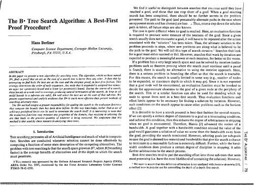
The B* Tree Search Algorithm: A Best-First Proof Proceduret - AITopics

The B* Tree Search Algorithm: A Best-FirstProof ProceduretHans BerlinerComputer Science Department, Carnegie—Mellon University,Pittsburgh, PA 15213, U.S.A.ABSTRACTIn this paper we present a new algorithm for searching trees. The algorithm, which we have namedB*, finds a proof that an arc at the root of a search tree is better than any other. It does this byattempting to find both the best arc at the root and the simplest proof, in best-first fashion. Thisstrategy determines the order of node expansion. Any node that is expanded is assigned two values:an upper (or optimistic) bound and a lower (or pessimistic) bound. During the course of a search,these bounds at a node tend to converge, producing natural termination of the search. As long as allnodal bounds in a sub-tree are valid, B* will select the best arc at the root of that sub-tree. Wepresent experimental and analytic evidence that B4. is much more effective than present methods ofsearching adversary trees.The B* method assigns a greater responsibility for guiding the search to the evaluation functionsthat compute the bounds than has been done before. In this way knowledge, rather than a set ofarbitrary predefined limits can be used to terminate the search itself It is interesting to note thatthe evaluation functions may measure any properties of the domain, thus resulting in selecting thearc that leads to the greatest quantity of whatever is being measured. We conjecture that thismethod is that used by chess masters in analyzing chess trees,1. IntroductionTree searching permeates all of Artificial Intelligence and much of what is computation.Searches are conducted whenever selection cannot be done effectively bycomputing a function of some state description of the competing alternatives. Theproblem with tree searching is that the search space grows as BD, where B (branchingfactor) is the average breadth of alternatives and D the depth to which the searchmust penetrate.This research was sponsored by the Defense Advanced Research Projects Agency (DOD),ARPA Order No. 3597, monitored by the Air Force Avionics Laboratory Under ContractF33615-78-C-1551.We find it useful to distinguish between searches that cor.iinue until they havereached a goal, and those that can stop short of a goal. When a goal reachingsearch has been completed, there should be no further secrets in the problempresented. The path to the goal (and presumably alternate paths in the case wherean opponent exists and has choices) are kno 1. Thus, once a step down the solutionpath is taken, all future steps are also known.The case is quite different when no goal is reached. Here, an evaluation functionis required to produce some measure of the nearness of the goal. Since a givensearch usually does not encounter a goal, it will have to be repeated after the actionassociated with the "solution" has been taken. Thus, the ultimate solution to theproblem proceeds in steps, where new problems are along what is believed to bethe path to the goal. We will call this type of search iterative.' Searches that lookfor a goal must either succeed or fail. However, searches that work by iteration areexpected to produce a meaningful answer at each iteration, for better or for worse.If a problem has a very large search space and can be solved by iteration (unlikeproblems such as theorem proving where the search must continue until a proofis found), there is usually no alternative to using the iterative approach. Here,there is a serious problem in bounding the effort so that the search is tractable.For this reason, the search is usually limited in some way (e.g., number of nodesto be expanded, or maximum depth to which it may go). Since it is not expectedthat a goal node will be encountered, an evaluation function must be invoked todecide the approximate closeness to the goal of a given node at the periphery ofthe search. This or a similar function can also be used for deciding which tipnode to sprout from next in a best—first search. Thus evaluation functions andeffort limits appear to be necessary for finding a solution by iteration. However,such conditions on the search appear to cause other problems such as the horizoneffect [2].It is desirable to have a search proceed in best—first fashion for several reasons.If we can specify a certain degree of closeness to a goal as a terminating condition,and achieve this condition, then this reduces the degree of arbitrariness in stoppingwhen no goal is encountered. Therefore, Harris [7] advanced the notion of abandwidth. A goal together with a bandwidth condition around the value of thegoal would guarantee a solution of value no worse than the bandwidth away fromthe goal, providing the search terminated. However, selecting goals (or sub-goalsin case the goal is deemed too remote) and bandwidths that give the search a chanceto terminate in a reasonable fashion is extremely difficult. Further, while the bandwidthcondition does produce a certain degree of discipline in stopping, it addsfurther arbitrariness to the search process.Best—first searches tend to put the searching effort into those suh-trees that seemmost promising (i.e. have the most likelihood of containing the solution). However,'We want to assure that this definition of iteration is not confused with iterative deepening 115].a method now in popular use for controlling the depth of a depth-first search.INH111:1001V .9CO

est-first searches require a great deal of bookkeeping for keeping track of allcompeting nodes, contrary to the great efficiencies possible in depth-first searches.Depth-first searches, on the other hand, tend to be forced to stop at inappropriatemoments thus giving rise to the horizon effect. They also tend to investigate hugetrees, large parts of which have nothing to do with any solution (since everypotential arc of the losing side must be refuted). However, these large trees sometimesturn up something that the evaluation functions would not have found werethey guiding the search. This method of discovery has become quite popular oflate, since new efficiencies in managing the search have been found [15]. At themoment the efficiencies and discovery potential of the depth-first methods appearto outweight what best-first methods have to offer. However, both methods havesome glaring deficiencies.FIG. 1.In the situation of Fig. I, both best-first and depth-first searches will expendtheir allotted effort and come to the conclusion that the arc labelled A is best.Clearly, no search is required for this conclusion, since it is the only arc from theroot. To overcome this waste of effort, the developers of performance programs(notably chess programs) test for this condition before embarking on any search_the other hand, would probably expend its entire effort in the sub-tree of arc A,and eventually come to the conclusion that it was best. These incongrqities requireno further explanation.2. The B* AlgorithmIn present methods for doing iterative searches, there is no natural way to stop thesearch. Further, for any given effort limit, the algorithm's idea of what is the bestarc at the root, may change so that each new effort increment could produce aradical change in the algorithm's idea of what is correct. To prevent this and toprovide for natural termination, the B* search provides that each node has twoevaluations: an optimistic one and a pessimistic one. Together, these provide arange on the values that are (likely) to be found in the node's sub-tree. Intuitively,these bounds delimit the area of uncertainty in the evaluation. If the evaluationsare valid bounds, the values in a given sub-tree will be within the range specifiedat the root of the sub-tree. As new nodes in a given sub-tree are expanded andthis information is backed up, the range of the root node of that sub-tree will begradually reduced until, if necessary, it converges on a single value. This featureof our method augurs well for the tractability of searches. In fact, a simple bestfirstsearch in the two valued system would converge if all bounds are valid.However, as we shall show, a B* search converges more rapidly.The domain of B* is both 1-person searches and 2-person (adversary) searches.We shall explain the B* algorithm using adversary searches, where one player triesto maximize a given function while the other tries to minimize it. In the canonicalcase where nodes have a single value [11, pp. 137-140], MAX is assumed to be onmove at the root, and the arc chosen at the root has a backed-up minimax valuethat is no worse than that of any other arc at the root. In the two valued systemthat we introduced above, this condition is slightly relaxed: MAX need only showthat the pessimistic value of an arc at the root is no worse than the optimistic value ofany of the other arcs at the root. This is the terminal condition for finding the bestarc.COSEARCH AND SEARCH REPRESENTATIONSFlo. 2.In Fig. 2 the situation is different as there Lae three legal successors to the rootnode. Numbers at the descendant nodes are intended to show how an evaluationfunction would appraise the relative merits of the three nodes. Here the depth-firstsearch has no recourse but to do its search, and (if the initial evaluation is reasonablycorrect) eventually report that arc A should be chosen. A best-first search onFio. 3. Start of a B* search.0710[30,15) [22, 83 [19,103We show the basic situation at the start of a 2-person ternary search tree inFig. 3. The optimistic and pessimistic values associated with any node are shownnext to it in brackets, the optimistic value being the leftmost of the pair. Thesevalues will be updated as the search progresses. In Fig. 3, it apvears that the leftmost

arc has the greatest potential for being the best. It should be noted that if this searchwere with single valued nodes and this were maximum depth, the search wouldterminate here without exploring the question of the uncertainty in the evaluation.In the case of B., there are no terminating conditions other than the one previouslyenunciated. When at the root, the B. search may pursue one of two strategies:(1) It may try to raise the lower bound of the leftmost (most optimistic) nodeso that it is not worse than the upper bound of any of its sibling nodes. We will callthis the PROVEBEST strategy.(2) It may try to lower the upper bounds of all the other nodes at depth 1, sothat none are better than the lower bound of the leftmost node. We will call thisthe DISPROVEREST strategy.In either case, the strategy will have to create a proof tree to demonstrate that ithas succeeded. We show the simplest cases of the alternate strategies in Figs. 4 and5. In the figures, the numbers inside the node symbols indicate the order of nodeFio. 4. The PROVEBEST strategy.Flo. 5. The DISPROVEREST strategy.15,30Es-6,9115 14-D o, is) [,6] [,

(1) The range (the number of discrete values) of the evaluation function wasvaried from 100 to 6400 by factors of four.(2) The width of branching was varied from 3 to 10 in increments of 1.Thus there are 32 basic conditions, and 50 tree searches were performed for eachcondition. For each such run a different search algorithm was tested. Any search thatpenetrated beyond depth 100, or which put more than 30,000 nodes into its nodesdictionary was declared intractable and aborted.Several observations could be made about the test data. In general, tree sizegrew with width. Range, on the other hand, turned out to be a non-monotonicfunction. Searches with the smallest and largest ranges required the least effort ingeneral. Searches of range 400 were hardly ever the largest for any given width andalgorithm, while searches of range 1600 were hardly ever the smallest for anygiven width and algorithm. We cannot interpret this result beyond it indicatingthat there seems to be a range value for which searches will require most effort andthat ranges above and below this will require less.We tested several distinct variations of the B* algorithm. These related to thecriteria for selecting the strategy at the root. The variations are explained below;although we did not test all combinations of these conditions.(I) Number of alternatives considered when making strategy decision at root.2 - Best plus one alternative.3 - Best plus two alternatives.A - All alternatives.(2) Criterion applied to decide strategy.D - If the sum of the squares of the depths from which the optimistic boundsof the alternatives had been backed up was less than the square of the depthfrom which the value of the best arc had been backed up, then the bestalternative was chosen, else the best arc. This favors exploring sub-trees whichhave not yet been explored deeply.R - Criterion information ("D" above or unity) was divided by the range ofthe node (thus favoring the searching of nodes with larger ranges).These alpha-numeric keys are used to label column headings in Table 1 to showwhich algorithm is being tested. BF indicates the results of running a best-firstsearch on the same data, and these are used as a base for comparison.The categories on the left are based upon how the best-first search did on a giventree. A given tree is in the intractable category, if any of the algorithms testedfound it intractable. The entries in the table indicate the ratio of effort, in terms ofnodes visited, compared to how the best-first search did on the set; e.g. 0.50 meansthat half the effort was required. All but the last row indicate the effort ratio; thelast row indicates the number of intractable searches for each version.TABLE 1. Effort compared to best-first for various implementations of B*Size/Alg BF 2D 2DR 3D AD 2DRX

and if the probability of this occurring is high enough, the probability of a stringof such occurrences can be quite high too. This was borne out when we did a runof the best algorithm with the additional proviso that any node for which the rangewas reduced to 2 or less, arbitrarily received a value equal to the mean of itsoptimistic and pessimistic value. For this change, the number of intractablesearches went from 71 to 4, and each of these was due to overflow of the nodesdictionary rather than exceeding the maximum depth. This method is somewhatreminiscent of Samuel's idea [12] of terminating search at a node when Alpha andBeta are very close together.To get another benchmark for comparing B*, we ran a depth—first alpha—betasearch on the same data. Here, we allowed the forward prune paradigm, since thebounds on any node were assumed valid. In a search without the two-value system,each node expansion could produce a value any distance from the value of itsparent. Since this cannot happen under the two-value scheme, it is logical to notsearch any node the range of which indicates it cannot influence the solution;thus the use of the forward prune paradigm. In order to prevent the search fromrunning away in depth, we used the iterative deepening approach [15] which goesto depth N, then to depth N+ 1, etc., until it finds a solution or becomes intractable.Searches were started with N = 1. The results showed that depth—first typicallyexpands three to seven times as many nodes as the BF algorithm. Although it didmanage to do a few problems in fewer nodes than the best B* algorithm, it wasunable to solve any problem of depth greater than 19, and became intractable onalmost twice as many searches as the BF algorithm. In contrast, the best B*algorithm solved some problems as deep as 94 ply, although it is conceivablethat shallower solutions existed.4. Considerations that Led to the Discovery of the AlgorithmIn the course of working on computer chess, we have had occasion to examinethe standard methods for searching adversary trees. The behavior of thesealgorithms appeared more cumbersome than the searches which I, as a chessmaster, believed myself capable of performing. The real issue was whether a welldefined algorithm existed for doing such searches.(1) Our initial motivation came from the fact that all searches that were notexpected to reach a goal required effort limits. Such effort limits, in turn, appearedto bring on undesirable consequences such as the horizon effect. While there arepatches to ameliorate such idiosyncracies of the search, the feeling that these werenot "natural" algorithms persisted.(2) There are two meaningful proposals to overcome the effort limit problem.Harris [7] proposed a bandwidth condition for terminating the search. However,this shifts the limiting quantity from a physical search effort limit, to a distancefrom the goal limit which, as indicated earlier, has other problems. Anotherattempt to avoid these problems was to use a set of maximum depths in a depthfirstsearch for terminating searches which qualified moves for other searches inthe chess program KAISSA (see [1]). For a set of maximum depths, first allmoves, then all material threatening moves plus captures, then all captures andchecks, and finally only captures were considered. With an effort limit for eachcategory of moves, it was hoped that everything of importance would somehow becovered. There are no reports of how this approach worked out, but it wouldappear to have the same essential limitations as all the other effort limited searches.This is borne out by the fact that the authors have now implemented another methodof searching for their program. In none of the existing tractable search proceduresis there a natural terminating condition without any parameters which specifyunder what conditions to halt.(3) We have noted that standard searches may at times investigate a very largenumber of nodes that have no apparent relevance to a solution. Consider thefollowing situation: If there is only one legal successor to the root node, anyiterative solution technique can easily check for this condition and indicate thisis the best successor without further analysis. However, if there is only one sensiblearc, a depth—first program will still insist on refuting all other arcs at the root tothe prescribed depth, while a best—first program may investigate the one good arcad infinitum. We have demonstrated these cases in Section 1. Usually, it is possibleto determine that the one sensible arc is best without going at all deep in thesearch. It appears that some essential ingredient is missing. We have felt for sometime that the notion of level of aspiration (as first put forward by Newell in [101)was the key to the proper construction. The alpha—beta search procedure appearsto have such a level of aspiration scheme. However, this scheme has an aspirationlevel for each side, and that only serves to bound those branches that can be apart of the solution. The correct level of aspiration specifies the value required fora "solution". We attempted such a construction in the search scheme of CAPS—II(see [3]), which relied heavily on notions of optimism, pessimism and aspiration.However, we performed depth limited depth—first searches in CAPS. Without thehest—first requirement there was no need to keep track of alternatives, nor tomaintain the optimistic and pessimistic values at each node.(4) We have always liked the way the search could be terminated at the rootnode, when the backed up (sure) value of one alternative is better than theoptimistic (static) values of all the other alternatives. This is the forward pruneparadigm, and while it can be used to keep the search from investigating branchesthat appear useless at any depth, it only terminates the search if applicable at theroot. In B*, the forward prune of all remaining alternatives at the root (whenPESSIM[CURNODE] OPTIM[ALTERN]) not only terminates the search,but it provides a logic for all actions taken in the search. Thus, when the final testsucceeds, a massive forward prune of all of the tree not connected with the solutionis effected.coSEARCH AND SEARCH REPRESENTATIONS

likelihood not measure what an optimality function would measure. Thus for chess,a good function might measure attack potential rather than distance to a mate,and for a graph traversal problem, ease of traversing a local sub-graph rather thantotal path length. This tends to partition the total task into small segments which(hopefully) would be bounded by what is being measured. Thus, in the chessexample the search would terminate when the attack issue is resolved (rather thancontinuing the analysis into the endgame), and in the path example the searchwould terminate once a local graph had been resolved with a convenient connectionto another part of the total graph. In this way the evaluation functions can keepmeasuring the next thing to be optimized, and thus lead the process through aseries of sub-optimal paths on the way to what is hoped to be the best ultimate goal.If new issues arise during a particular search, and De Groot presents some evidencethat they do in chess searches, humans change their aspiration level (which couldmean changing the evaluation function). We present analytic evidence for suchchanges in [4].We have constructed reasonable bounding functions for chess tactics, althoughwe did not then know of the B. algorithm [3]. The key for such constructions, isthat one side's optimism is the other's pessimism. For instance, our evaluationfunction calculates the optimistic value of a tactical move to be the current materialbalance plus the sum of all our recognized threats against material. The pessimisticvalue is the material balance minus the sum of all the opponent's recognized threats.When evaluation function estimates do not validly bound the actual value of anode, errors in arc selection can occur. However, there is no reason why these shouldbe more severe than errors produced by any other search technique using anestimating function which is applied at leaf nodes that are not terminal in thedomain per se. Thus, if an arc at the root is chosen because an estimate was in errorsomewhere in the tree, this would be no different than in searches with a singleevaluation function. If the error was detected prior to termination, data from oursimulations seem to indicate that small and infrequent intrusions of this type(which would happen when relatively good bounding functions do exist) have littleeffect on the magnitude of the search effort.The issue of when a B. search fails to terminate is more serious and could stillstand further investigation. In cases where the range of the best node at the rootremains overlapped with the ranges of at least one of its sibling nodes even aftera considerable search, several options are possible. One could select the arc withthe greatest average value, or temper this with some function of the depth ofinvestigation of each competing arc. Such contingencies probably arise in humansearches ard are resolved by humans in such situations by various means that wehave yet to understand. I am particularly struck by a quote from former WorldChess Champion Alexander Alekhin in [6, p. 409] : "Well, in case of timepressure I would play 1. B x N/5". A clear case of using an external criterion toresolve some small remaining uncertainty.Unfortunately, very little appears to have been done toward making a scienceof the construction of sensitive evaluation functions, since the highly significantwork of Samuels [12, 13]. We have been investigating how such evaluationfunctions can be constructed of many layers of increasingly more complex primitivesin connection with the 8-puzzle and backgammon [5]. In the latter greatamounts of knowledge need to be brought to bear, since search is not practicalbecause of a very large branching factor.6. Comparison to other Search AlgorithmsIt is interesting to compare the basic features of B. with those of well-known searchalgorithms. Consider the As search algorithm [II]. It could easily operate under thetwo value system in a mode that is satisfied to find the best arc at the root, and thecost of the path without finding the complete path itself. This algorithm would beequivalent to B. using only the PROVEBEST strategy, and being able to haltsearch on a branch only when a goal was reached or if the upper and lower boundson the branch became equal; i.e. the cost of the path is known. Another step in thedirection of iteration would be to only use the PROVEBEST strategy and allowthe search to halt when a best node at the root had been identified. In this mode theexact cost of the path would not be known. This produces the best—first algorithmused for the column headed BF in Table I. Finally, the full-fledged B. algorithmworking with both strategies discovers the best node without the exact cost of thepath. However, it does enough shallow searching so that it explores considerablyfewer nodes than any of the algorithms described above.Having the two strategies without the two value system has no meaning at all,since there is no way of pronouncing one node at the root better than any otherwithout having an effort limit. Just using a depth—first iterative deepening procedure,although it spreads the search over the shallower portions of the searchtree, investigates too many non-pertinent nodes.Finally, it should be noted that the optimistic and pessimistic values at a nodecorrespond exactly to alpha and beta in an alpha—beta minimax search. That isthey delimit the range of acceptable values that can be returned from their sub-tree.7. SummaryThere are two things that distinguish the B. algorithm from other known treesearch procedures:(1) The optimistic and pessimistic value system allows for termination of asearch without encountering a goal node, and without any effort limit.(2) The option to exercise either of two search strategies allows the search tospread its effort through the shallowest portion of a tree where it is least expensive,instead of being forced to pursue the best alternative to great depths, or pursue allalternatives to the same depth.I SEARCH AND SEARCH REPRESENTATIONS

In selecting a strategy, it is good to consider the present range of a node, and thedepth from which its current bounds have come. This allows some gauging of thecost of employing a particular strategy. Further, domain-dependent knowledgeassociated with an evaluation (not merely its magnitude), would no doubt also aidin strategy selection.I have had a number of discussion with colleagues about whether B. is a Branchand Bound (BB) algorithm. The view that it is has support in that some BBalgorithms do employ best-first methods and some do use upper and lowerbounds to produce their effects. The BB technique derives its main effect byeliminating the search of branches that can not contain the solution. B. will neverknowingly visit such branches either. In 13*, superceded nodes can be (and are inour implementation) permanently eliminated from the search as a matter of course.However, in our view, B. is definitely not a BB algorithm. The main strength ofthe 13* algorithm is the ability to pursue branches that are known to not be best,and no other algorithm that we know of can opt for such a strategy. Therefore, weassert 13* is quite different from the class referred to as BB algorithms. The readermay wish to judge for himself by perusing a comprehensive reference such as [9].There are a number of issues left for investigation: (1) it is important to discoverhow to construct good bounding functions; (2) more light should be shed on thequestion of how much of an effect is caused when the value of a new node is notwithin the bounds of its parent; (3) there seems to be a more optimal strategy thanalways pursuing the best branch lower in the tree.Given the fact that all search techniques are limited by the accuracy of the evaluationsof leaf nodes, B. appears to expand fewer nodes than any other techniqueavailable for doing iterative searches. B. achieves its results because it is continuallyaware of the status of alternatives and exactly what is required to prove one alternativebetter than the rest. In this it seems very similar to the underlying methodthat humans exibit in doing game tree searches, and we conjecture that it is indeedthis method that the 13* algorithm captures.Appendix I. How to Generate Canonical Trees of Uniform WidthWe here show how to generate canonical trees which are independent of the orderof search. We note that a tree can receive a unique name by specifying the rangeof values at its root, the width (number of immediate successors at each node),and the iteration number for a tree of this type. To find a unique name for eachnode in such a tree, we note that if we assign the name "0" to the root, and havethe immediate descendants of any node be named(parentname a width + 1),(parentname * width +2),-(parentname a width + width)then this provides a unique naming scheme. Now it is self-evident that the boundson a node that has not yet been sprouted from must be a function of its position inthe tree (name) and the name of the tree. Thus, if we initialize the random numbergenerator that assigns values to the immediate descendants of a node as a 11onof its original bounds, its name, the width, and the iteration number, then thedescendants of node "X" will look the same for all trees with the same initialparameters, regardless of the order of search or whether a node is actually everexpanded. The actual function we use to initialize the random number generatoris (parentname + width)* (iterationnumber +range). This avoids initializing atzero since width and range are never zero. The bounds of the parent node serve asbounds on the range of values that the random number generator is allowed toproduce.ACKNOWLEDGMENTThe author wishes to acknowledge the help of the following persons who provided assistance indiscussing the properties of the algorithm, improvement in its formulation, and improvement inthe readability of this paper: Allen Newell, Herbert Simon, Charles Leiserson, Andrew Palay,John Gaschnig, Jon Bentley, and the referees, whose comments were most helpful.REFERENCES1. Adelson-Velskiy, G. M., Arlasarov, V. L. and Donskoy, M. V., Some methods of controllingthe tree search in chess programs, Artificial Intelligence 6(4) (1975).2. Berliner, H. J., Some necessary conditions for a master chess program, Proceedings of the 3rdInternational Joint Conference on Artificial Intelligence (August 1973) 77-85.3. Berliner, H. J., Chess as problem solving: The development of a tactics analyzer, Dissertation,Comput. Sci. Dept., Carnegie-Mellon University (March 1974).4. Berliner, H. J., On the use of domain-dependent descriptions in tree searching, in: Jones,A. K. (Ed.), Perspectives on Computer Science (Academic Press, New York, 1977).5. Berliner, H. J., BKG - A program that plays backgammon, Comput. Sci. Dept., Carnegie-Mellon University (1977).6. De Groot, A. D., Thought and Choice in Chess (Mouton and Co., Der Haag, 1965).7. Harris, L., The heuristic search under conditions of error, Artificial Intelligence, 5 (1974)217-234.8. Harris, L. R., The heuristic search: An alternative to the alpha-beta minimax procedure,in: Frey, P. (Ed.), Chess Skill in Man and Machine (Springer-Verlag, Berlin, 1977).9. Lawler, E. L. and Wood, D. E., Branch-and-bounds methods: A survey, Operations Res. 14(1966) 699-719.10. Newell, A., The chess machine: An example of dealing with a complex task by adaptation,Proceedings Western Joint Computer Conference (1955) 101-108.11. Nilsson, N. J., Problem-Solving Methods in Artificial Intelligence (McGraw-Hill, New York,1971).12. Samuel, A. L., Some studies in machine learning using the game of checkers, IBM J. Res.. Develop. 3 (1959) 210-229.13. Samuel, A. L., Some studies in machine learning using the game of checkers, II - RecentProgress, IBM J. Res. Develop. (1967) 601-617.14. Schofield, P. D. A., Complete solution of the 'Eight-puzzle', in: Collins, N. L. and Michie, D.(Eds.), Machine Intelligence 1 (American Elsevier Publishing Co., New York, 1967).15. Slate, D. J. and Atkin, L. R., CHESS 4.5 - The Northwestern University Chess Program,in: Frey, P. (Ed.), Chess Skill in Man and Machine (Springer-Verlag, Berlin, 1977).WHIR:1091V .9 3H1