Physics 562: Statistical Mechanics Spring 2002, James P. Sethna ...

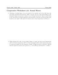
van der Waals WaterPressure (dynes/cm 2 )6×10 85×10 84×10 83×10 82×10 85005505756006256507007501×10 8050 100 150 200 250 300Volume per Mole (cm 3 )Figure 6.2.1: Pressure versus volume for a van der Waals approximation to H 2 O,with a =0.5507 Joules meter cubed per mole squared (a =1.51957 × 10 −35 ergscm 3 per molecule), and b =3.04×10 −5 meter cubed per mole (b =5.04983×10 −23cm 3 per molecule), from http://www.ac.wwu.edu/∼vawter/PhysicsNet/Topics/-Thermal/vdWaalEquatOfState.html.5

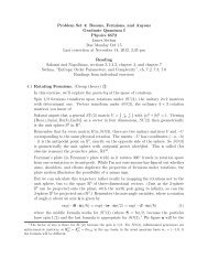
Chemical Potential µ(ρ) (10 -12 ergs/molecule)-0.6-0.61-0.62-0.63-0.64Coarse-Grained Free Energyµ(ρ) for H 20 at 373K, p=1.5x10 7 dynes/cm 2-0.650 0.005 0.01 0.015 0.02 0.025 0.03Density (moles/cm 3 )Figure 6.2.2: Chemical potential µ[ρ] of water fit with the van der Waals equation,as in figure 6.2.1, at T = 373K and P =1.5 × 10 7 dynes/cm 2 .(e) According to the caption to figure 6.2.2, what is the vdW approximation to the vaporpressure at 373K = 100C? Atmospheric pressure is around one bar = 0.1MPa =10 6 dynes/cm 2 . How close is the vdW approximation to the true vapor pressure ofwater? (Hint: what happens when the vapor pressure hits atmospheric pressure?)If µ 0 is the common chemical potential shared by the water and the vapor at this temperature,the extra Gibbs free energy for a density fluctuation ρ(x) is∫∆G = ρ(x)(µ[ρ(x)] − µ 0 ) d 3 x. (6.2.4)(f) At room temperature, the interface between water and water vapor is very sharp: perhapsa molecule thick. Use the vdW model for the chemical potential (figure (6.2.2))and equation (6.2.4) to roughly estimate the surface tension of water (the extra Gibbsfree energy per unit area, roughly the barrier height times thickness). How does youranswer compare with the measured value at the boiling point, 59 dynes/cm?6

(6.3) Hysteresis Model: Scaling and Exponent Equalities.Find a Windows machine. Download Matt Kuntz’ hysteresis simulation from our courseWeb site http://www.physics.cornell.edu/sethna/teaching/562/Work.html. ∗Run it with the default parameters (two dimensions, R =0.9, 1000×1000) You can usethe center buttons in the upper right of the subwindow and main window to make themexpand to fill the screen.The simulation is a simple model of magnetic hysteresis, described in detail in the CracklingNoise paper distributed in class; see also http://www.lassp.cornell.edu/sethna/hysteresis.The spins s i begin all pointing down, and flip upward as the external field H grows fromminus infinity, depending on the spins of their neighbors and a local random field h i .Theflipped spins are colored as they flip, with spins in the same avalanche sharing the samecolor. An avalanche is a collection of spins all triggered from the same original spin. Inthe parameter box, the Disorder is the ratio R of the root-mean-square width √ 〈h 2 i 〉 tothe ferromagnetic coupling J between spins:R = √ 〈h 2 〉/J. (6.3.1)(a) Examine the M(H) curve for our model (the fourth button, marked with the S curve)and the dM/dH curve (the fifth button, marked with a spiky curve). The individualavalanches should be visible on the first graph as jumps, and the second graph asspikes. This kind of time series (a set of spikes or pulses with a broad range of sizes)we hear as crackling noise. You can go to our site http://simscience.org/crackling/to hear the noise resulting from our model, as well as crackling noise we’ve assembledfrom crumpling paper, from fires and Rice Krispies c○ , and from the earth (earthquakesin 1995, sped up to audio frequencies).We claim in three dimensions that there is a phase transition in the dynamical evolutionin our model. Well below R c ∼ 2.16 (for the cubic lattice), one large avalanche flips mostof the spins. Well above R c all avalanches are fairly small: at very high disorder each spinflips individually. We measure the critical disorder as the point, as L →∞,whereonefirst finds spanning avalanches, which extend from one side of the simulation to the other.Does this transition also occur in two dimensions? We don’t know for sure, but let’s explorethe question.(b) Simulating two-dimensional systems of length L = 100, locate a rough estimate forR c . You can do multiple runs by setting the #Runs: watch them on the fly andcount the number that look mostly monochromatic. Now check your answer for the∗Source for an earlier version is available at http://www.lassp.cornell.edu/sethna/hysteresis/code/.7

critical disorder by going to a larger system size, say L = 1000: do a few runs at thecritical disorder you estimated for L = 100. Are there important finite size effects?Several papers calculate scaling exponents in two dimensions for small systems aroundL = 200. (They had computers that weren’t as fast as yours, and didn’t have clever, speedyalgorithms.) Just as you saw in part (b), their measured critical disorder was clearly wrong:when we simulated larger systems at their estimated R c , all of our avalanches were muchsmaller than the system size (although comparable in size to their entire simulation). Ourcurrent best guess is that the critical disorder may actually be zero in two dimensions (justlike the critical temperature for the one-dimensional Ising model is zero in one dimension),but we don’t have any definitive answers.For later use, in the directory where the program HysteresisWin.exe resides, add a foldernamed data and in it put a directory named average. The program will save data files intothose directories (but won’t create them for you). Check Output Data Files on the dialogbox before starting the long runs.Simulations in three dimensions are slower and less exciting: let’s explore the self-similarstructures in two dimensions. Do ten runs (setting Run # to ten so we can look at the averages)in two dimensions at L = 1000 and R =0.8. Take a look at the avalanche size distribution(the A button). The horizontal axis is the log of the size S of the avalanche (numberof spins flipped) and the vertical axis is the probability D(S) that a given avalanche is ofthat size. (Matt never worked out how to put axes on his graphs, but he did put in thelog-log grid: the left-hand side is at x =1.)(c) Does the avalanche size distribution look like a power law? Over how many decades?Estimate the power law relating the probability to the size D(S) ∼ S x .The C button shows the spin-spin correlation function: the horizontal axis is distance x,and the vertical axis is the probability C(x) that an avalanche initiated at a point x 0 willextend and flip a spin x 1 adistancex = √ (x 1 − x 0 ) 2 away.(d) Set Run # to two and run at R =1andR = 2. Plot the three average correlationfunctions, stored in the folder average. (The names of the files should tell you whichlength L and disorder R they simulated; the first column in the file gives the meansize S in the histogram, the second column gives the value of C(S, R), and the thirdcolumn is the statistical error estimated from the runs you did.)We need to do at least one scaling collapse. In two dimensions the scaling behavior stillconfuses us, so this could be considered research. Let’s scale the correlation function toextract the correlation length. We expect the correlation function in two dimensions tohave the scaling formC(x, R) =x −(2+β/ν) C (x/ξ(R)) , (6.3.2)where in three dimensions ξ(R) ∼ (R − R c ) −ν . In two dimensions, we believe β/ν =0.We don’t know the functional form of ξ(R) in two dimensions (we believe it might grow8

exponentially as exp(A/R 2 ), but it might be a conventional power law or something elseentirely). So, in our scaling collapse, we’ll treat each of the three ξ(R) valuesasanindependent variable, and use the collapse to measure the function.(e) Do a scaling collapse: plot x 2+β/ν C(x, R) versusx/ξ(R) for the three curves youplotted in part (d). Vary the three constants ξ(2.0), ξ(1.0), and ξ(0.8) to best collapsethe data: you might want, for example, to make the peaks line up at x/ξ =1. Plotξ(R). If you have the energy, compare it to what you would expect from an exponentialform ξ = ξ 0 exp(A/R 2 ) and a power-law form ξ = ξ 0 (R − R c ) −ν .9

(6.4A) The Renormalization Group and the Central Limit Theorem: ShortVersion.“A Mean-Field Spin Glass with Short-Range Interactions,” J. T. Chayes, L. Chayes, J. P.Sethna, and D. J. Thouless, Commun. Math. Phys. 106, 41 (1986).If you’re familiar with the renormalization group and Fourier transforms, this problem canbe stated very quickly. If not, you’re probably better off doing the long version (followingpage).Write a renormalization-group transformation T taking the space of probability distributionsinto itself, that takes two random variables, adds them, and rescales the width by thesquare root of two. Show that the Gaussian of width σ is a fixed point. Find the eigenfunctionsf n and eigenvectors λ n of the linearization of T at the fixed point. (Hint: it’seasy in Fourier space.) Describe physically what the relevant and marginal eigenfunctionsrepresent. By subtracting the fixed-point distribution from a binomial distribution, findthe leading correction to scaling, as a function of x. Which eigenfunction does it represent?Why is the leading irrelevant eigenvalue not dominant here?10

(6.4B) The Renormalization Group and the Central Limit Theorem: Long Version.“A Mean-Field Spin Glass with Short-Range Interactions,” J. T. Chayes, L. Chayes, J. P.Sethna, and D. J. Thouless, Commun. Math. Phys. 106, 41 (1986).In this problem, we will develop a renormalization group in function space. We’ll be usingmaps (like our renormalization transformation T ) that take a function ρ of x into anotherfunction of x; we’ll write T [ρ] as the new function, and T [ρ](x) as the function evaluatedat x. We’ll also make use of the Fourier transformF[ρ](k) =∫ ∞−∞e −ikx ρ(x) dx;F maps functions of x into functions of k.notation: ˜ρ = F[ρ], so for exampleWhen convenient, we’ll also use the tildeρ(x) = 1 ∫ ∞e ikx ˜ρ(k) dk; (6.4.1)2π −∞The central limit theorem states that the sum of many independent random variablestends to a Gaussian, whatever the original distribution might have looked like. Thatis, the Gaussian distribution is the fixed point function for large sums. When summingmany random numbers, the details of the distributions of the individual random variablesbecomes unimportant: simple behavior emerges. We’ll study this using the renormalizationgroup, largely created here at Cornell by Michael Fisher and Ken Wilson, with initial ideasby Leo Kadanoff (then at Brown). There are four steps in the procedure:1. Coarse grain. Remove some fraction (usually half) of the degrees of freedom. Here, wewill add pairs of random variables: the probability distribution for sums of N independentrandom variables of distribution f is the same as the distribution for sums of N/2 randomvariables of distribution f ∗ f, where∗ denotes convolution.(a.) Argue that if ρ(x) is the probability that a random variable has value x, that the probabilitydistribution of the sum of two random variables drawn from this distributionis the convolutionC[ρ](x) =(ρ ∗ ρ)(x) =∫ ∞−∞ρ(x − y)ρ(y)dy. (6.4.2)Show thatF[C[ρ]](k) =(˜ρ(k)) 2 , (6.4.3)the well-known statement that the Fourier transform of the convolution is the productof the Fourier transforms.11

(d) Show using equation (6.4.7) that the transforms of the eigenfunctions satisfyf˜n (k) =(2/λ n ) ˜ρ ∗ (k/ √ 2) f ˜ n (k/ √ 2). (6.4.9)4. Find the Eigenvalues and Calculate the Universal Critical Exponents.(e) Show that ˜f n (k) =k n ˜ρ ∗ (k) is the Fourier transform of an eigenfunction (i.e., thatitsatisfies (6.4.9).) What is the eigenvalue λ n ?All the relevant and marginal operators are dangerous! We need to make sure physicallythat they correspond to things we understand physically.(f) The eigenfunction f 0 (x) with the biggest eigenvector corresponds to an unphysicalperturbation: why? The next two eigenfunctions f 1 and f 2 have important physicalinterpretations. Show that ρ ∗ + ɛf 1 to lowest order is equivalent to a shift in the meanof ρ, andρ ∗ + ɛf 2 is a shift in the standard deviation σ of ρ ∗ .All other eigenfunctions should have eigenvalues λ n less than one. This means that aperturbation in that direction will shrink under the renormalization–group transformation:non-Gaussian wiggles f n (x) in the distribution will die out:T N (ρ ∗ + ɛf n ) − ρ ∗ ∼ λ N n ɛf n. (6.4.10)The next two eigenfunctions are easy to write in Fourier space, but slightly complicatedto Fourier transform into real space. They aref 3 (x) ∝ ρ ∗ (x)(3x/σ − x 3 /σ 3 ) (6.4.11)f 4 (x) ∝ ρ ∗ (x)(3 − 6x 2 /σ 2 + x 4 /σ 4 )Eigenvalues of the linearization about the fixed point of absolute value less than one areirrelevant. Microscopic deviations in these eigendirections will die away at long lengths.(h) How many relevant variables are there for our renormalization–group transformation?How many marginal variables (with eigenvalue one) are there?For second order phase transitions, temperature is typically a relevant direction, witheigenvalue greater than one. This implies that the deviation of the temperature from thecritical point grows under coarse–graining: on longer and longer length scales the systemlooks farther and farther from the critical point. Specifically, if the temperature is justabove the phase transition, the system appears “critical” on length scales smaller thanthe correlation length, but on larger length scales the effective temperature has moved farabove the transition temperature and the system looks fully disordered.In our problem, the relevant directions are simple: they change the width and the meansof the Gaussian. In a formal sense, we have a line of fixed points and an unstable direction:13

the renormalization group doesn’t tell us that by subtracting the mean and rescaling thewidth all of the distributions would converge to the same Gaussian.Corrections to Scaling and Coin Flips. Does anything really new come from all thisanalysis? One nice thing that comes out is the leading corrections to scaling. The fixedpoint of the renormalization group explains the Gaussian shape of the distribution of Ncoin flips in the limit N →∞, but the linearization about the fixed point gives a systematicunderstanding of the corrections to the Gaussian distribution for large but not infinite N.Usually, the largest eigenvalues are the ones which dominate. In our problem, consideradding a small perturbation to the fixed point f ∗ along the two leading irrelevant directionsf 3 and f 4 :ρ(x) =ρ ∗ (x)+ɛ 3 f 3 (x)+ɛ 4 f 4 (x). (6.4.12)What happens when we add 2 l of our random variables to one another (correspondingto l applications of our renormalization group transformation T )? The new distributionshould be given byT l (ρ)(x) ∼ ρ ∗ (x)+λ l 3 ɛ 3f 3 (x)+λ l 4 ɛ 4f 4 (x). (6.4.13)Since 1 >λ 3 >λ 4 , the leading correction should be dominated by the perturbation withthe largest eigenvalue.(i) Plot the difference between the binomial distribution of N coin flips and a Gaussianof the same mean and width, for N =10andN = 20. Does it approach one of theeigenfunctions?(j) Why didn’t a perturbation along f 3 (x) dominate the asymptotics? What symmetryforced ɛ 3 = 0? Should flips of a biased coin break this symmetry?We should mention that there are other fixed points for sums of many random variables.If the variance of the original probability distribution is infinite, one can get so-called Levydistributions.14