A Method to Estimate the Human Capital from Sample Surveys on ...
A Method to Estimate the Human Capital from Sample Surveys on ...
A Method to Estimate the Human Capital from Sample Surveys on ...

You also want an ePaper? Increase the reach of your titles
YUMPU automatically turns print PDFs into web optimized ePapers that Google loves.
A <str<strong>on</strong>g>Method</str<strong>on</strong>g> for The Estimati<strong>on</strong> of The Distributi<strong>on</strong> of<str<strong>on</strong>g>Human</str<strong>on</strong>g> <str<strong>on</strong>g>Capital</str<strong>on</strong>g> <str<strong>on</strong>g>from</str<strong>on</strong>g> <str<strong>on</strong>g>Sample</str<strong>on</strong>g> <str<strong>on</strong>g>Surveys</str<strong>on</strong>g> <strong>on</strong> Income andWealthGiorgio Vittadini, University of Bicocca Milan, Italy Camilo Dagum, University of Bologna, Italy and University ofOttawa, Canada, Pietro Giorgio Lovaglio, University of Bicocca-Milan, Italy, Michele Costa, University of Bologna,Italy.Giorgio Vittadini, Department of Statistics, University of Bicocca-Milan,Via Bicocca degli Arcimboldi 8, 20126MILAN, ITALY.KEY WORDS: <str<strong>on</strong>g>Human</str<strong>on</strong>g> <str<strong>on</strong>g>Capital</str<strong>on</strong>g>,Latent Variable, Pls, Lisrel,Optimal ScalingIntroducti<strong>on</strong>This paper proposes a method for estimating <str<strong>on</strong>g>the</str<strong>on</strong>g> 1983U.S. household distributi<strong>on</strong> of <str<strong>on</strong>g>Human</str<strong>on</strong>g> <str<strong>on</strong>g>Capital</str<strong>on</strong>g>. From<str<strong>on</strong>g>the</str<strong>on</strong>g> statistical point of view, <str<strong>on</strong>g>the</str<strong>on</strong>g> HC is defined as aLatent Variable measured by a set of observed mixedindica<str<strong>on</strong>g>to</str<strong>on</strong>g>rs in a Path Analysis Model. The HC estimatesc<strong>on</strong>sider <str<strong>on</strong>g>the</str<strong>on</strong>g> definiti<strong>on</strong>s advanced for a Latent Variablein a Path Analysis with respect <str<strong>on</strong>g>to</str<strong>on</strong>g> formative andreflective indica<str<strong>on</strong>g>to</str<strong>on</strong>g>rs.The set of indica<str<strong>on</strong>g>to</str<strong>on</strong>g>rs and <str<strong>on</strong>g>the</str<strong>on</strong>g>ir links with HCThe c<strong>on</strong>cept of <str<strong>on</strong>g>Human</str<strong>on</strong>g> <str<strong>on</strong>g>Capital</str<strong>on</strong>g> (HC), <str<strong>on</strong>g>the</str<strong>on</strong>g>oretically andsystematically developed over <str<strong>on</strong>g>the</str<strong>on</strong>g> last 50 years (Mincer1958, 1970; Becker 1962, 1964 and Schultz 1959,1961) has been estimated in literature by ei<str<strong>on</strong>g>the</str<strong>on</strong>g>r <str<strong>on</strong>g>the</str<strong>on</strong>g>retrospective (Kendrick 1976; Eisner, 1985) orprospective methods (Jorgens<strong>on</strong> and Fraumeni 1989).The first, dealing with <str<strong>on</strong>g>the</str<strong>on</strong>g> cost of producti<strong>on</strong>, isinsufficient for various reas<strong>on</strong>s, because it does nottake in<str<strong>on</strong>g>to</str<strong>on</strong>g> account <str<strong>on</strong>g>the</str<strong>on</strong>g> social costs, such as publicinvestment in educati<strong>on</strong>, <str<strong>on</strong>g>the</str<strong>on</strong>g> variables c<strong>on</strong>cerning homec<strong>on</strong>diti<strong>on</strong>s and community envir<strong>on</strong>ments, and <str<strong>on</strong>g>the</str<strong>on</strong>g>genetic c<strong>on</strong>tributi<strong>on</strong> <str<strong>on</strong>g>to</str<strong>on</strong>g> HC, including health c<strong>on</strong>diti<strong>on</strong>s(Dagum and Vittadini 1996). Moreover, <str<strong>on</strong>g>the</str<strong>on</strong>g> actualeffects of <str<strong>on</strong>g>the</str<strong>on</strong>g> investment in HC <strong>on</strong> <str<strong>on</strong>g>the</str<strong>on</strong>g> income andwealth of <str<strong>on</strong>g>the</str<strong>on</strong>g> households are not c<strong>on</strong>sidered.In <str<strong>on</strong>g>the</str<strong>on</strong>g> prospective method <str<strong>on</strong>g>the</str<strong>on</strong>g> HC can be defined as <str<strong>on</strong>g>the</str<strong>on</strong>g>present actuarial value of an individual’s expectedincome related <str<strong>on</strong>g>to</str<strong>on</strong>g> his skill, acquired abilities, andeducati<strong>on</strong> (Dagum and Slottje 2000). However, <str<strong>on</strong>g>the</str<strong>on</strong>g>prospective method reduces <str<strong>on</strong>g>the</str<strong>on</strong>g> HC investment <str<strong>on</strong>g>to</str<strong>on</strong>g> itsm<strong>on</strong>etary value in terms of an assumed flow of income,and it ignores <str<strong>on</strong>g>the</str<strong>on</strong>g> amount of investment in educati<strong>on</strong>,job training and o<str<strong>on</strong>g>the</str<strong>on</strong>g>r investments. It is also difficult <str<strong>on</strong>g>to</str<strong>on</strong>g>predict future income.We now present a new methodology <str<strong>on</strong>g>to</str<strong>on</strong>g> estimate <str<strong>on</strong>g>the</str<strong>on</strong>g>distributi<strong>on</strong> of HC in families, giving greater emphasis<str<strong>on</strong>g>to</str<strong>on</strong>g> ec<strong>on</strong>omic issues because <str<strong>on</strong>g>the</str<strong>on</strong>g> definiti<strong>on</strong> of HCinvolves both its investment amounts <strong>on</strong> families andits effect <strong>on</strong> income. In this case, instead of quantitativefinancial indica<str<strong>on</strong>g>to</str<strong>on</strong>g>rs, we have a composite set ofqualitative and quantitative indica<str<strong>on</strong>g>to</str<strong>on</strong>g>rs (Table 1) with<str<strong>on</strong>g>the</str<strong>on</strong>g> Path Analysis diagram showing <str<strong>on</strong>g>the</str<strong>on</strong>g>ir causal links.The ”indirect” set of indica<str<strong>on</strong>g>to</str<strong>on</strong>g>rs Γ =(x 2, x 3, x 6, y 8, y 9, y 10,y 11, y 12, y 13 ) involved in <str<strong>on</strong>g>the</str<strong>on</strong>g> Path Analysis is composedof a set of causal links between <str<strong>on</strong>g>the</str<strong>on</strong>g>mselves and a set ofindica<str<strong>on</strong>g>to</str<strong>on</strong>g>rs [Ψ=(x 1, x 4, x 5, x 7, y 1, y 2, y 3, y 4, y 5, y 6, y 7, y 15 )]and y 14 (<str<strong>on</strong>g>to</str<strong>on</strong>g>tal wealth), which measure <str<strong>on</strong>g>the</str<strong>on</strong>g> investment ineducati<strong>on</strong> and are directly c<strong>on</strong>nected with HC in (2).As proposed in statistical literature (Tenenhaus, 1995),<str<strong>on</strong>g>the</str<strong>on</strong>g>se indica<str<strong>on</strong>g>to</str<strong>on</strong>g>rs can be defined as formative indica<str<strong>on</strong>g>to</str<strong>on</strong>g>rsbecause <str<strong>on</strong>g>the</str<strong>on</strong>g>y “form” or “cause” <str<strong>on</strong>g>the</str<strong>on</strong>g> multidimensi<strong>on</strong>alc<strong>on</strong>struct HC in equati<strong>on</strong> (2). HC is a “c<strong>on</strong>sequence”of <str<strong>on</strong>g>the</str<strong>on</strong>g> investment in educati<strong>on</strong>. It is measured by a se<str<strong>on</strong>g>to</str<strong>on</strong>g>f formative indica<str<strong>on</strong>g>to</str<strong>on</strong>g>rs F = (y 14 ,Ψ)The most important formative indica<str<strong>on</strong>g>to</str<strong>on</strong>g>rs are years ofeducati<strong>on</strong>, years of full time and part time employment,and wealth. Marital status, gender, regi<strong>on</strong> and age areinvolved as well, because <str<strong>on</strong>g>the</str<strong>on</strong>g> actual value ofinvestment in HC is influenced by <str<strong>on</strong>g>the</str<strong>on</strong>g>se pers<strong>on</strong>al andenvir<strong>on</strong>mental c<strong>on</strong>diti<strong>on</strong>s.The effects <strong>on</strong> income of <str<strong>on</strong>g>the</str<strong>on</strong>g> households HC andwealth are presented in (3). Therefore y 17 can beclassified as reflective indica<str<strong>on</strong>g>to</str<strong>on</strong>g>r, because it reflects HC,in <str<strong>on</strong>g>the</str<strong>on</strong>g> sense that it is a c<strong>on</strong>sequence of <str<strong>on</strong>g>the</str<strong>on</strong>g> amount andtype of <str<strong>on</strong>g>the</str<strong>on</strong>g> investment in educati<strong>on</strong>. Wealth (y 14 ) isboth a formative indica<str<strong>on</strong>g>to</str<strong>on</strong>g>r and an independent cause ofincome.The ec<strong>on</strong>ometric specificati<strong>on</strong> and analysis was madeby Dagum (1994) and Dagum et al. (2003).
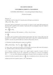
Indirect Indica<str<strong>on</strong>g>to</str<strong>on</strong>g>rs Γx 2 =H Gender; x 3 = H Race; x 6 = S Age; y 5 = H Yearsof Not Full-Time Work; y 7 = S Years of Not Full-Time Work; y 8 = H Job Status; y 9 = H Occupati<strong>on</strong>;y 10 = H Industry; y 11 = S Job Status; y 12 = S Occupati<strong>on</strong>y 13 = S IndustryFormative indica<str<strong>on</strong>g>to</str<strong>on</strong>g>rs F = (Ψ, y 14 )Ψ: x 1 = H Age; x 4 = Regi<strong>on</strong> ;x 5 = H Marital Status;x 7 = S Gender; y 1 = H Years of Schooling;y 2 = S Years of Schooling; y 3 = Number of Children;y 4 = H Years of Full-Time Work;y 6 = S Years of Full-Time Work; y 14 = HouseholdTotal Wealth; y 15 = Household Total Debts.Reflective indica<str<strong>on</strong>g>to</str<strong>on</strong>g>ry 17 = Household IncomeH: Household Head;S: SpouseTable 1 Observed indica<str<strong>on</strong>g>to</str<strong>on</strong>g>rsThe statistical definiti<strong>on</strong> of <str<strong>on</strong>g>the</str<strong>on</strong>g> LV HCWe have already stated (Dagum and Vittadini 1996)that, <str<strong>on</strong>g>from</str<strong>on</strong>g> <str<strong>on</strong>g>the</str<strong>on</strong>g> statistical point of view, HC can beexpressed as an LV. But <str<strong>on</strong>g>the</str<strong>on</strong>g>re are different ways an LVcan be defined. Traditi<strong>on</strong>ally, a variable can be definedas an LV if <str<strong>on</strong>g>the</str<strong>on</strong>g> equati<strong>on</strong>s cannot be manipulated in<str<strong>on</strong>g>to</str<strong>on</strong>g>expressing <str<strong>on</strong>g>the</str<strong>on</strong>g> variable as a functi<strong>on</strong> of manifestvariables (Bentler 1982). In o<str<strong>on</strong>g>the</str<strong>on</strong>g>r words, in thisdefiniti<strong>on</strong>, an LV is a fac<str<strong>on</strong>g>to</str<strong>on</strong>g>r that underlies and causesreflective indica<str<strong>on</strong>g>to</str<strong>on</strong>g>rs and accounts for <str<strong>on</strong>g>the</str<strong>on</strong>g>ir observedvariance in a measurement model (typically <str<strong>on</strong>g>the</str<strong>on</strong>g> fac<str<strong>on</strong>g>to</str<strong>on</strong>g>rmodel) given <str<strong>on</strong>g>the</str<strong>on</strong>g> effects of o<str<strong>on</strong>g>the</str<strong>on</strong>g>r explicative indica<str<strong>on</strong>g>to</str<strong>on</strong>g>rs(in this case <str<strong>on</strong>g>the</str<strong>on</strong>g> reflective indica<str<strong>on</strong>g>to</str<strong>on</strong>g>r Income, given <str<strong>on</strong>g>the</str<strong>on</strong>g>effect of <str<strong>on</strong>g>the</str<strong>on</strong>g> explicative indica<str<strong>on</strong>g>to</str<strong>on</strong>g>r wealth in equati<strong>on</strong>(3)). O<str<strong>on</strong>g>the</str<strong>on</strong>g>rwise we can define HC as a latent variablecaused and measured (with errors) by a linearcombinati<strong>on</strong> of <str<strong>on</strong>g>the</str<strong>on</strong>g> formative indica<str<strong>on</strong>g>to</str<strong>on</strong>g>rs F in equati<strong>on</strong>(2). Finally we can propose a third, more complete,definiti<strong>on</strong> of an LV, as in this case where it isc<strong>on</strong>nected with both formative and reflectiveindica<str<strong>on</strong>g>to</str<strong>on</strong>g>rs in a Path Diagram. Hence <str<strong>on</strong>g>the</str<strong>on</strong>g> latent variableHC can be defined as a linear combinati<strong>on</strong> offormative indica<str<strong>on</strong>g>to</str<strong>on</strong>g>rs F that best fits <str<strong>on</strong>g>the</str<strong>on</strong>g> reflectiveindica<str<strong>on</strong>g>to</str<strong>on</strong>g>r earning income, as in equati<strong>on</strong>s (2)-(3).The proposed methodologyThis approach completes <str<strong>on</strong>g>the</str<strong>on</strong>g> methodology proposed byDagum and Slottje (2000) where <str<strong>on</strong>g>the</str<strong>on</strong>g>y combine azerodimensi<strong>on</strong>al latent variable approach (part A) andan actuarial ma<str<strong>on</strong>g>the</str<strong>on</strong>g>matical approach (part B).The Latent Variable approach proposes a newmethodology able <str<strong>on</strong>g>to</str<strong>on</strong>g> obtain <str<strong>on</strong>g>the</str<strong>on</strong>g> zerodimensi<strong>on</strong>al HClatent variable, <str<strong>on</strong>g>the</str<strong>on</strong>g>n transforms <str<strong>on</strong>g>the</str<strong>on</strong>g> estimated latentvariable in<str<strong>on</strong>g>to</str<strong>on</strong>g> an accounting m<strong>on</strong>etary value, and finallyestimates <str<strong>on</strong>g>the</str<strong>on</strong>g> mean value of HC. The Path Analysisand <str<strong>on</strong>g>the</str<strong>on</strong>g> Latent Variable Approach are shown inFigure1.The Actuarial Ma<str<strong>on</strong>g>the</str<strong>on</strong>g>matical approach starts with <str<strong>on</strong>g>the</str<strong>on</strong>g>actuarial estimati<strong>on</strong>, in m<strong>on</strong>etary values, of <str<strong>on</strong>g>the</str<strong>on</strong>g> averagehuman capital by age of ec<strong>on</strong>omic units and finallyestimates <str<strong>on</strong>g>the</str<strong>on</strong>g> average of <str<strong>on</strong>g>the</str<strong>on</strong>g> populati<strong>on</strong> in m<strong>on</strong>etaryunits. The syn<str<strong>on</strong>g>the</str<strong>on</strong>g>sis gives <str<strong>on</strong>g>the</str<strong>on</strong>g> final HC estimati<strong>on</strong> anddistributi<strong>on</strong> of American Household.INDIRECTINDICATORS ΓINDICATORS OFHOUSEHOLD INVESTMENT INEDUCATION:FORMATIVE INDICATORS ΨH S YEARS OF SCHOOLING;H S YEARS OF TOTAL TIME WORK; HAGE;REGION; H MARITAL STATUS;S GENDER; NUMBER OF CHILDRENHCWEALTH y 14LATENT VARIABLE HUMAN CAPITALFigureINDICATOR OF EFFECTS OFHC: REFLECTIVEINDICATOR INCOME y 17Figure 1: Path Analysis and Latent Variablesapproachy 1 = g 1 (x 1 , x 3 , x 4 , x 5 ) + u 1y 2 = g 2 (x 1 , x 2 , x 3 , x 4 , x 5 , y 1 ) + u 2y 3 = g 3 (x 1 , x 3 , x 4 , x 5 , y 1 ) + u 3y 4 = g 4 (x 1 , x 2 , x 3 , x 4 , x 5 , y 2 , y 3 ) + u 4y 5 = g 5 (x 1 , x 2 , x 3 , x 4 , x 5 , y 1 , y 4 ) + u 5y 6 = g 6 (x 2 , x 3 , x 4 , x 5 , x 6 , y 2 , y 3 , y 4 ) + u 6y 7 = g 7 (x 2 , x 4 , x 5 , x 6 , y 2 , y 5 , y 6 )+ u 7y 8 = g 8 (x 1 , x 2 , x 3 , x 4 , x 5 , y 1 , y 3 , y 4 ) + u 8 (1)y 9 = g 9 (x 1 , x 2 , x 3 , y 8 ) + u 9(1)y 10 = g 10 (x 2 , x 3 , x 4 , y 1 , y 4 , y 5 , y 9 ) + u 10y 11 = g 11 (x 1 , x 2 , x 4 , x 5 , x 6 , y 2 , y 3 , y 6 , y 9 ) + u 11y 12 = g 12 (x 1 , x 2 , x 4 , x 5 , x 6 , y 2 , y 3 , y 9 , y 11 ) + u 12y 13 = g 13 (x 3 , x 4 , y 6 , y 12 ) + u 13y 14 = g 14 (x 4 , y 1 , y 2 , y 4 , y 7 , y 8 , y 9 , y 10 , y 11 , y 12 , y 13 )+ u 14y 15 = g 15 (x 1, x 3 , x 4 , y 1 , y 2 , y 3 , y 4 , y 9 , y 10 , y 12 , y 14 ) + u 15HC = Fg = [y 14 ,Ψ] g + u 16 (2)
y 17 = y 14 k 1 + HC k 2 + u 17 (3)The Latent Variable Approach: previous proposalThe traditi<strong>on</strong>al proposal in statistical literature is <str<strong>on</strong>g>to</str<strong>on</strong>g>obtain <str<strong>on</strong>g>the</str<strong>on</strong>g> latent variable HC as a latent cause whichunderlies observed indica<str<strong>on</strong>g>to</str<strong>on</strong>g>rs by means of Fac<str<strong>on</strong>g>to</str<strong>on</strong>g>rAnalysis . In this case starting <str<strong>on</strong>g>from</str<strong>on</strong>g> (3), we obtain:Q y14y 17 = HC k 2 # + u 17 (4)where Q y14=I– Py 14is <str<strong>on</strong>g>the</str<strong>on</strong>g> orthog<strong>on</strong>al complement of<str<strong>on</strong>g>the</str<strong>on</strong>g> column spaces of y14 with Py 14= y14 (y 14 ′ y 14 ) -1 y 14 ′.By means of Fac<str<strong>on</strong>g>to</str<strong>on</strong>g>r Analysis we obtain HC as <str<strong>on</strong>g>the</str<strong>on</strong>g>latent cause of <str<strong>on</strong>g>the</str<strong>on</strong>g> reflective indica<str<strong>on</strong>g>to</str<strong>on</strong>g>r earning income.First of all, in this way we define <str<strong>on</strong>g>the</str<strong>on</strong>g> HC withouttaking in<str<strong>on</strong>g>to</str<strong>on</strong>g> account <str<strong>on</strong>g>the</str<strong>on</strong>g> amount of investment ineducati<strong>on</strong> measured by <str<strong>on</strong>g>the</str<strong>on</strong>g> formative indica<str<strong>on</strong>g>to</str<strong>on</strong>g>rs F.Sec<strong>on</strong>dly, under general c<strong>on</strong>diti<strong>on</strong>s, given earningincome Wealth Q y14y17, <str<strong>on</strong>g>the</str<strong>on</strong>g> parameter k # 2 is notidentified and <str<strong>on</strong>g>the</str<strong>on</strong>g> scores of <str<strong>on</strong>g>the</str<strong>on</strong>g> latent variable HC arenot unique. In a Fac<str<strong>on</strong>g>to</str<strong>on</strong>g>rial or in a Structural model when<str<strong>on</strong>g>the</str<strong>on</strong>g> expected values of latent variables are null, <str<strong>on</strong>g>the</str<strong>on</strong>g>identificati<strong>on</strong> problem is essentially whe<str<strong>on</strong>g>the</str<strong>on</strong>g>r or notvec<str<strong>on</strong>g>to</str<strong>on</strong>g>r ϑ of parameters and of variances andcovariances of latent variables and errors is uniquelydetermined by <str<strong>on</strong>g>the</str<strong>on</strong>g> covariance matrix Σ of indica<str<strong>on</strong>g>to</str<strong>on</strong>g>rswhose elements are σ ij . In o<str<strong>on</strong>g>the</str<strong>on</strong>g>r words if a vec<str<strong>on</strong>g>to</str<strong>on</strong>g>r ϑ canbe uniquely determined <str<strong>on</strong>g>from</str<strong>on</strong>g> Σ ( and <str<strong>on</strong>g>the</str<strong>on</strong>g>refore if Σ isgenerated by <strong>on</strong>e and <strong>on</strong>ly <strong>on</strong>e vec<str<strong>on</strong>g>to</str<strong>on</strong>g>r ϑ) <str<strong>on</strong>g>the</str<strong>on</strong>g>n solving<str<strong>on</strong>g>the</str<strong>on</strong>g> equati<strong>on</strong>s σ ij = σ ij (ϑ), i ≤ j (with p manifestvariables, <str<strong>on</strong>g>the</str<strong>on</strong>g>re are ½ p(p + 1) equati<strong>on</strong>s in n(θ)unknown parameters), or a subset of <str<strong>on</strong>g>the</str<strong>on</strong>g>m, this vec<str<strong>on</strong>g>to</str<strong>on</strong>g>rof parameter is identified and <str<strong>on</strong>g>the</str<strong>on</strong>g> whole model is said<str<strong>on</strong>g>to</str<strong>on</strong>g> be identified; o<str<strong>on</strong>g>the</str<strong>on</strong>g>rwise it is not. Anders<strong>on</strong> andRubin showed that a necessary c<strong>on</strong>diti<strong>on</strong> foridentificati<strong>on</strong> is that <str<strong>on</strong>g>the</str<strong>on</strong>g> number of equati<strong>on</strong>s σ ij =σ ij (ϑ), i ≤ j must be greater than <str<strong>on</strong>g>the</str<strong>on</strong>g> order of <str<strong>on</strong>g>the</str<strong>on</strong>g> vec<str<strong>on</strong>g>to</str<strong>on</strong>g>rϑ: p ≥ 2t n(θ)+1. However, since <str<strong>on</strong>g>the</str<strong>on</strong>g> equati<strong>on</strong>s aboveare often n<strong>on</strong>-linear, <str<strong>on</strong>g>the</str<strong>on</strong>g> soluti<strong>on</strong> is often complicatedand tedious, and explicit soluti<strong>on</strong>s for all ϑ’s seldomexist. “No general and practically useful necessary andsufficient c<strong>on</strong>diti<strong>on</strong>s for identificati<strong>on</strong> are available”(Everitt 1984).If a model is not completely identified, appropriaterestricti<strong>on</strong>s may be imposed <strong>on</strong> ϑ <str<strong>on</strong>g>to</str<strong>on</strong>g> make itidentifiable. The choice of restricti<strong>on</strong>s may affect <str<strong>on</strong>g>the</str<strong>on</strong>g>interpretati<strong>on</strong> of <str<strong>on</strong>g>the</str<strong>on</strong>g> results of an estimated model.Under general c<strong>on</strong>diti<strong>on</strong>s for <str<strong>on</strong>g>the</str<strong>on</strong>g> Fac<str<strong>on</strong>g>to</str<strong>on</strong>g>r Model, if wedo not c<strong>on</strong>sider a few very restricted cases in whichc<strong>on</strong>diti<strong>on</strong>s for identifiability are studied analytically,e.g. where <str<strong>on</strong>g>the</str<strong>on</strong>g> endogenous variables are measuredwithout error (Geraci 1976), <str<strong>on</strong>g>the</str<strong>on</strong>g> problem cannot beresolved. In practice, it is suggested (Jöreskog, 1981b)that “The identificati<strong>on</strong> problem can be studied <strong>on</strong> acase by case basis by examining <str<strong>on</strong>g>the</str<strong>on</strong>g> equati<strong>on</strong>s”,choosing <str<strong>on</strong>g>the</str<strong>on</strong>g> restricti<strong>on</strong>, not <strong>on</strong>ly in number but also inpositi<strong>on</strong>, in order <str<strong>on</strong>g>to</str<strong>on</strong>g> obtain unique soluti<strong>on</strong>s. This isalso true in <str<strong>on</strong>g>the</str<strong>on</strong>g> case of local identifiability of <str<strong>on</strong>g>the</str<strong>on</strong>g>parameters (Wegge 1965, 1991 Fisher 1976,Ro<str<strong>on</strong>g>the</str<strong>on</strong>g>nberg 1971, Geraci 1976, Bekker and Pollock1986, Shapiro 1985, Bekker 1989, 1991, Wegge andFeldman, 1983).In our case, we have <strong>on</strong>e equati<strong>on</strong> σ ij = σ ij (ϑ):σ = (k 2 # ) 2 + σ u17 (5)y Q y1417With two unknown values, <str<strong>on</strong>g>the</str<strong>on</strong>g> square of <str<strong>on</strong>g>the</str<strong>on</strong>g>#parameter k 2 (k # 2 ) 2 and <str<strong>on</strong>g>the</str<strong>on</strong>g> variance of <str<strong>on</strong>g>the</str<strong>on</strong>g> error u 17(σ u17 ). Therefore, under general c<strong>on</strong>diti<strong>on</strong>s, when <str<strong>on</strong>g>the</str<strong>on</strong>g>Reliability Ratio between σ and (k2 # ) 2 isQ y14 y17unknown or <str<strong>on</strong>g>the</str<strong>on</strong>g> variance of <str<strong>on</strong>g>the</str<strong>on</strong>g> error σ u17 orInstrumental Variables are not available, <str<strong>on</strong>g>the</str<strong>on</strong>g> model (4)is not identifiable (Fuller, 1987).Regarding <str<strong>on</strong>g>the</str<strong>on</strong>g> problem of indeterminacy we can verifythat, under general c<strong>on</strong>diti<strong>on</strong>s, <str<strong>on</strong>g>the</str<strong>on</strong>g> matrix of observedindica<str<strong>on</strong>g>to</str<strong>on</strong>g>rs is less than <str<strong>on</strong>g>the</str<strong>on</strong>g> matrix of latent scores anderrors. Therefore, it can be dem<strong>on</strong>strated that even if<str<strong>on</strong>g>the</str<strong>on</strong>g> model is identified <str<strong>on</strong>g>the</str<strong>on</strong>g> latent scores areindeterminate. There are infinite sets of latent scoresfor <str<strong>on</strong>g>the</str<strong>on</strong>g> same identified model. It can be proved thatsome of <str<strong>on</strong>g>the</str<strong>on</strong>g>m can be ei<str<strong>on</strong>g>the</str<strong>on</strong>g>r negatively correlated <str<strong>on</strong>g>to</str<strong>on</strong>g>each o<str<strong>on</strong>g>the</str<strong>on</strong>g>r (Reiersol 1950; Guttmann 1955; Anders<strong>on</strong>and Rubin 1956; Lawley and Maxwell 1963; Joreskog1967; Sch<strong>on</strong>emann and Wang 1972; Sch<strong>on</strong>emann andSteiger 1978; Steiger 1979; Sch<strong>on</strong>emann and Haagen1987). In this case, given y17 and k # 2 , we canQ y14obtain infinite set of scores of HC; moreover some of<str<strong>on</strong>g>the</str<strong>on</strong>g>m can be negatively correlated.An alternative proposal is given by <str<strong>on</strong>g>the</str<strong>on</strong>g> Partial LeastSquares <str<strong>on</strong>g>Method</str<strong>on</strong>g> (<str<strong>on</strong>g>from</str<strong>on</strong>g> here <strong>on</strong> referred <str<strong>on</strong>g>to</str<strong>on</strong>g> as PLS):PLS provides estimates of parameters g in (2) definingand estimating an LV “by deliberate approximati<strong>on</strong> asa linear aggregate of its observed indica<str<strong>on</strong>g>to</str<strong>on</strong>g>rs” (Wold1982). In this definiti<strong>on</strong> <str<strong>on</strong>g>the</str<strong>on</strong>g> HC appearing in (2) is nota fac<str<strong>on</strong>g>to</str<strong>on</strong>g>r of <str<strong>on</strong>g>the</str<strong>on</strong>g> observed reflective indica<str<strong>on</strong>g>to</str<strong>on</strong>g>rs (3) but anunobserved <str<strong>on</strong>g>the</str<strong>on</strong>g>oretical c<strong>on</strong>struct, approximated by alinear combinati<strong>on</strong> of observed formative indica<str<strong>on</strong>g>to</str<strong>on</strong>g>rs,e.g. following equati<strong>on</strong> (2):H Ĉ = F ĝ(6)where HĈ is <str<strong>on</strong>g>the</str<strong>on</strong>g> proxy obtained by reducing <str<strong>on</strong>g>the</str<strong>on</strong>g> loss ofinformati<strong>on</strong> with respect <str<strong>on</strong>g>to</str<strong>on</strong>g> <str<strong>on</strong>g>the</str<strong>on</strong>g> unobservable HC.There are two alternatives for obtaining <str<strong>on</strong>g>the</str<strong>on</strong>g> soluti<strong>on</strong>s ofHĈ in (6) by means of <str<strong>on</strong>g>the</str<strong>on</strong>g> PLS. The PLS mode A isbased <strong>on</strong> iterative multivariate regressi<strong>on</strong>s of <str<strong>on</strong>g>the</str<strong>on</strong>g> LV’s<strong>on</strong> <str<strong>on</strong>g>the</str<strong>on</strong>g> observed indica<str<strong>on</strong>g>to</str<strong>on</strong>g>rs; <str<strong>on</strong>g>the</str<strong>on</strong>g>refore, if <str<strong>on</strong>g>the</str<strong>on</strong>g>re is a singleLV, it cannot be used, because it causes “circularsoluti<strong>on</strong>s” without improvements in <str<strong>on</strong>g>the</str<strong>on</strong>g> iterati<strong>on</strong>s. ThePLS mode B is based <strong>on</strong> simple iterative regressi<strong>on</strong>s <strong>on</strong><str<strong>on</strong>g>the</str<strong>on</strong>g> observed indica<str<strong>on</strong>g>to</str<strong>on</strong>g>rs F=(y 14 ; Ψ). It can be provedthat <str<strong>on</strong>g>the</str<strong>on</strong>g> estimate of HĈ is equivalent <str<strong>on</strong>g>to</str<strong>on</strong>g> <str<strong>on</strong>g>the</str<strong>on</strong>g> firstprincipal comp<strong>on</strong>ent of F (Wold 1982). Therefore wehave in (6):HĈ = Fv 1 = y 14 v 11 + Ψ v 12 (7)
where F =(y 14 , Ψ) and v 1 ′ =(v 11 , v 12 )′ is <str<strong>on</strong>g>the</str<strong>on</strong>g> firsteigenvec<str<strong>on</strong>g>to</str<strong>on</strong>g>r of F′F, HĈ is <str<strong>on</strong>g>the</str<strong>on</strong>g> first principal comp<strong>on</strong>en<str<strong>on</strong>g>to</str<strong>on</strong>g>f F after its standardizati<strong>on</strong> <str<strong>on</strong>g>to</str<strong>on</strong>g> unit variance(Var(HĈ)=1), v 11 c<strong>on</strong>tains <str<strong>on</strong>g>the</str<strong>on</strong>g> element of <str<strong>on</strong>g>the</str<strong>on</strong>g> firsteigenvec<str<strong>on</strong>g>to</str<strong>on</strong>g>r c<strong>on</strong>nected with y 14 , v 12 is <str<strong>on</strong>g>the</str<strong>on</strong>g> sub-vec<str<strong>on</strong>g>to</str<strong>on</strong>g>r ofv 1 c<strong>on</strong>nected with Ψ.First of all, <str<strong>on</strong>g>the</str<strong>on</strong>g> estimate HĈ of HC does not take in<str<strong>on</strong>g>to</str<strong>on</strong>g>account <str<strong>on</strong>g>the</str<strong>on</strong>g> actual effects of <str<strong>on</strong>g>the</str<strong>on</strong>g> investment in HC <strong>on</strong><str<strong>on</strong>g>the</str<strong>on</strong>g> income and wealth of <str<strong>on</strong>g>the</str<strong>on</strong>g> households.Sec<strong>on</strong>dly, also <str<strong>on</strong>g>from</str<strong>on</strong>g> <str<strong>on</strong>g>the</str<strong>on</strong>g> statistical point of view, <str<strong>on</strong>g>the</str<strong>on</strong>g>reare some general critique about <str<strong>on</strong>g>the</str<strong>on</strong>g> soluti<strong>on</strong>s obtainedby means of PLS (Garthwaite 1994).In this case, in particular, every soluti<strong>on</strong> that can beobtained in (3) starting <str<strong>on</strong>g>from</str<strong>on</strong>g> (7) is logicallyinc<strong>on</strong>sistent. In effect, substituting HC^ obtained by(7) in (4) we obtain:and <str<strong>on</strong>g>from</str<strong>on</strong>g> (7) we have:Q y14y 17 = HĈ k 2 # + u 17 (8)k # 2 = HC^′ Qy y17 =(y 14 v 11 + Ψ v 12 )′ 14Q y14y17=v 12 ′ Ψ ′ Qy y 17 (9)14#<str<strong>on</strong>g>from</str<strong>on</strong>g> which k 2 cannot c<strong>on</strong>sider <str<strong>on</strong>g>the</str<strong>on</strong>g> whole HCc<strong>on</strong>tributi<strong>on</strong> <str<strong>on</strong>g>to</str<strong>on</strong>g> earned income y17 because, byQ y14definiti<strong>on</strong>, <str<strong>on</strong>g>the</str<strong>on</strong>g> indirect c<strong>on</strong>tributi<strong>on</strong> of Wealth <strong>on</strong>Income y 17 by means of HĈ is null.However, if we c<strong>on</strong>sider equati<strong>on</strong> (3) where <str<strong>on</strong>g>the</str<strong>on</strong>g>dependent variable is Income y 17 we have, substitutingHĈ obtained by (7):y 17 = [y 14 , y 14 , Ψ] ⎜ ⎜⎛10⎜⎝00 ⎞⎟ ⎛ k1⎞v11⎟⎜⎟v⎟ ⎝k2 ⎠12 ⎠+ u 17 (10)In (10) we observe <str<strong>on</strong>g>the</str<strong>on</strong>g> presence of collinearity betweenregressors, and if we join <str<strong>on</strong>g>the</str<strong>on</strong>g> parameters, we cannotdivide <str<strong>on</strong>g>the</str<strong>on</strong>g> direct c<strong>on</strong>tributi<strong>on</strong> of Invested Wealth <strong>on</strong>Income and <str<strong>on</strong>g>the</str<strong>on</strong>g> indirect c<strong>on</strong>tributi<strong>on</strong> of Wealth bymeans of HĈ. In effect,y 17 = y 14 [ k 1 + v 11 k 2 ] + Ψv 12 k 2 + u 17 (11)The Latent Variable Approach: a new proposalIt has been shown that <str<strong>on</strong>g>the</str<strong>on</strong>g> soluti<strong>on</strong>s obtained by meansof <str<strong>on</strong>g>the</str<strong>on</strong>g> Fac<str<strong>on</strong>g>to</str<strong>on</strong>g>r Model are not unique and that <str<strong>on</strong>g>the</str<strong>on</strong>g>soluti<strong>on</strong>s obtained by <str<strong>on</strong>g>the</str<strong>on</strong>g> PLS <str<strong>on</strong>g>Method</str<strong>on</strong>g> are not logicallyc<strong>on</strong>sistent (Lovaglio 2003). In order <str<strong>on</strong>g>to</str<strong>on</strong>g> overcome thisproblem, a soluti<strong>on</strong> can be found in <str<strong>on</strong>g>the</str<strong>on</strong>g> use of all <str<strong>on</strong>g>the</str<strong>on</strong>g>informati<strong>on</strong> embedded in <str<strong>on</strong>g>the</str<strong>on</strong>g> Path Analysis model (2)(3). In this way, <str<strong>on</strong>g>the</str<strong>on</strong>g> HC is not previously obtained inequati<strong>on</strong> (3) but, respecting <str<strong>on</strong>g>the</str<strong>on</strong>g> ec<strong>on</strong>omic relati<strong>on</strong>shipsis simultaneously obtained <str<strong>on</strong>g>from</str<strong>on</strong>g> reflective andformative indica<str<strong>on</strong>g>to</str<strong>on</strong>g>rs. In this perspective, observing <str<strong>on</strong>g>the</str<strong>on</strong>g>Path Analysis model (2) and (3), HC can be defined asa multidimensi<strong>on</strong>al c<strong>on</strong>struct approximated by <str<strong>on</strong>g>the</str<strong>on</strong>g>linear combinati<strong>on</strong> of its formative indica<str<strong>on</strong>g>to</str<strong>on</strong>g>rs (y 14 ,Ψ)that better fits <str<strong>on</strong>g>the</str<strong>on</strong>g> <strong>on</strong>ly reflective indica<str<strong>on</strong>g>to</str<strong>on</strong>g>rthat we can define as <str<strong>on</strong>g>the</str<strong>on</strong>g> earned income effect.Therefore we have <str<strong>on</strong>g>from</str<strong>on</strong>g> (2) :Premultiplying <str<strong>on</strong>g>the</str<strong>on</strong>g> equati<strong>on</strong> (13) by F and taking in<str<strong>on</strong>g>to</str<strong>on</strong>g>account (2) we obtain:yQ y14 17,Q y14y 17 = Fgk 2 +u 17 =F k 3 +u 17 where k 3 = gk 2 (12)In (12) we obtain k * 3by means of an ordinary LeastSquares Regressi<strong>on</strong> of Q y y17 <strong>on</strong> F. The k * 143vec<str<strong>on</strong>g>to</str<strong>on</strong>g>rc<strong>on</strong>tains <str<strong>on</strong>g>the</str<strong>on</strong>g> effects of <str<strong>on</strong>g>the</str<strong>on</strong>g> formative indica<str<strong>on</strong>g>to</str<strong>on</strong>g>rs F <strong>on</strong>earned income yQ y14 17:k * -13= g k 2 = S F F′ Qy y17 where S F = F′F (13)14F k * 3= F g k 2 = HC k 2 (14)Remembering that Var(HC) = S HC =1 we reach:* *2k3′SF k3= k2 S HC k 2 = k 2(15)From (15) we obtain k 2 * , <str<strong>on</strong>g>the</str<strong>on</strong>g> effect of HC <strong>on</strong> incomenet of wealth yQ y14 17:k 2 * = [(y 17 ′ Q y14F SF -1 F′ Q y14y17] 1/2 == [y 17 ′ Qy PF y14Q y14 17] 1/2 (16)where P F =F(F′ F) -1 F′.Therefore, <str<strong>on</strong>g>from</str<strong>on</strong>g> (13) and (16), we obtain g*, <str<strong>on</strong>g>the</str<strong>on</strong>g> effec<str<strong>on</strong>g>to</str<strong>on</strong>g>f <str<strong>on</strong>g>the</str<strong>on</strong>g> formative indica<str<strong>on</strong>g>to</str<strong>on</strong>g>rs F <strong>on</strong> HC:g*= k * / k =3*2= [y 17 ′ Q y14PF Q y14y 17 ] -1/2 S -1 F F′ Q y14y17 (17)At this point <str<strong>on</strong>g>from</str<strong>on</strong>g> (2) and (17) we obtain <str<strong>on</strong>g>the</str<strong>on</strong>g> estimati<strong>on</strong>of HC scores (HC*) :HC* = F g* (18)The Latent Variable Approach: mixed indica<str<strong>on</strong>g>to</str<strong>on</strong>g>rsIn our case, some of <str<strong>on</strong>g>the</str<strong>on</strong>g> formative indica<str<strong>on</strong>g>to</str<strong>on</strong>g>rs arecategorical.Therefore we partiti<strong>on</strong> <str<strong>on</strong>g>the</str<strong>on</strong>g> vec<str<strong>on</strong>g>to</str<strong>on</strong>g>r of formativeindica<str<strong>on</strong>g>to</str<strong>on</strong>g>rs in<str<strong>on</strong>g>to</str<strong>on</strong>g> quantitative (c<strong>on</strong>tained in <str<strong>on</strong>g>the</str<strong>on</strong>g> column ofmatrix F q ) and categorical indica<str<strong>on</strong>g>to</str<strong>on</strong>g>rs F c in order <str<strong>on</strong>g>to</str<strong>on</strong>g>obtain c<strong>on</strong>sistent soluti<strong>on</strong>s with <str<strong>on</strong>g>the</str<strong>on</strong>g> quantitative case.We express <str<strong>on</strong>g>the</str<strong>on</strong>g> equati<strong>on</strong> (2) in <str<strong>on</strong>g>the</str<strong>on</strong>g> following way:HC = F c g c + F q g q + u 16 , (F c = x 3 , x 4 , x 5 , x 7 ) (19)where F = (F c ,F q ), g = (g c ,g q )
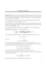
We avoid <str<strong>on</strong>g>the</str<strong>on</strong>g> approach of <str<strong>on</strong>g>the</str<strong>on</strong>g> Item Fac<str<strong>on</strong>g>to</str<strong>on</strong>g>r Model(Chris<str<strong>on</strong>g>to</str<strong>on</strong>g>fferss<strong>on</strong> 1975; Olss<strong>on</strong> 1979; Mu<str<strong>on</strong>g>the</str<strong>on</strong>g>n andChris<str<strong>on</strong>g>to</str<strong>on</strong>g>fferss<strong>on</strong> 1981) c<strong>on</strong>sisting of a Fac<str<strong>on</strong>g>to</str<strong>on</strong>g>r Modelwith qualitative and categorical indica<str<strong>on</strong>g>to</str<strong>on</strong>g>rs. In effect,this model increases <str<strong>on</strong>g>the</str<strong>on</strong>g> difficulties c<strong>on</strong>cerning <str<strong>on</strong>g>the</str<strong>on</strong>g>original fac<str<strong>on</strong>g>to</str<strong>on</strong>g>r model. The n<strong>on</strong> realistic hypo<str<strong>on</strong>g>the</str<strong>on</strong>g>sis of<str<strong>on</strong>g>the</str<strong>on</strong>g> normality of qualitative indica<str<strong>on</strong>g>to</str<strong>on</strong>g>rs, and somerestrictive assumpti<strong>on</strong>s, determine an underestimati<strong>on</strong>of <str<strong>on</strong>g>the</str<strong>on</strong>g> true correlati<strong>on</strong> between different indica<str<strong>on</strong>g>to</str<strong>on</strong>g>rs, <str<strong>on</strong>g>the</str<strong>on</strong>g>asymp<str<strong>on</strong>g>to</str<strong>on</strong>g>tical dis<str<strong>on</strong>g>to</str<strong>on</strong>g>rti<strong>on</strong>s of standard errors and <str<strong>on</strong>g>the</str<strong>on</strong>g> n<strong>on</strong>chi-square distributi<strong>on</strong> of goodness of fit statistics(Quiroga 1991; Vittadini 1999).We choose <str<strong>on</strong>g>the</str<strong>on</strong>g> multidimensi<strong>on</strong>al scaling methodALSOS, which alternatevely estimates, in separatesteps <str<strong>on</strong>g>the</str<strong>on</strong>g> parameter vec<str<strong>on</strong>g>to</str<strong>on</strong>g>r g and quantifies <str<strong>on</strong>g>the</str<strong>on</strong>g>categorical indica<str<strong>on</strong>g>to</str<strong>on</strong>g>rs F c by means of a uniquealgorithm., inside a specified model, <str<strong>on</strong>g>the</str<strong>on</strong>g> MultipleRegressi<strong>on</strong> Analysis (De Leeuw, Young and Takane1976; De Leeuw and Young 1978; De Leeuw and VanRijckevorsel 1980; Young 1981; Gifi 1981; Keller andWaansbeek 1983).We adapt this methodology in order <str<strong>on</strong>g>to</str<strong>on</strong>g> obtain <str<strong>on</strong>g>the</str<strong>on</strong>g> HC*,with <str<strong>on</strong>g>the</str<strong>on</strong>g> same methodology proposed in <str<strong>on</strong>g>the</str<strong>on</strong>g>quantitative case. If at <str<strong>on</strong>g>the</str<strong>on</strong>g> first step we arbitrarilychoose <str<strong>on</strong>g>the</str<strong>on</strong>g> parameters g c (0)* , we obtain <str<strong>on</strong>g>the</str<strong>on</strong>g> firstquantificati<strong>on</strong> of F c (0)* F cF c (0)* = F c g c (0)* with F (0)* = (F c (0* ,F q ) (20)At this point, we introduce F (0)* in (11) usingequati<strong>on</strong>s (13)-(17), we obtain <str<strong>on</strong>g>the</str<strong>on</strong>g> first estimates of <str<strong>on</strong>g>the</str<strong>on</strong>g>(1)* (1)*parameters k 2 , k 3 , g (1)* = (g (1)* c , g * q ) and bymeans of (18) <str<strong>on</strong>g>the</str<strong>on</strong>g> first estimates of HC, HC (1)* . Using(1)(1)g c in (19) we obtain a new quantificati<strong>on</strong> F c ofindica<str<strong>on</strong>g>to</str<strong>on</strong>g>rs F c . The iterative process c<strong>on</strong>tinues until we* *have no more changes in k 2 , k 3 , g * , HC*, F*Therefore, in this way, <str<strong>on</strong>g>the</str<strong>on</strong>g> case of mixed indica<str<strong>on</strong>g>to</str<strong>on</strong>g>rs istreated similarly <str<strong>on</strong>g>to</str<strong>on</strong>g> <str<strong>on</strong>g>the</str<strong>on</strong>g> case of quantitative indica<str<strong>on</strong>g>to</str<strong>on</strong>g>rs.<str<strong>on</strong>g>Human</str<strong>on</strong>g> <str<strong>on</strong>g>Capital</str<strong>on</strong>g> in m<strong>on</strong>etary units.As a quantitative multidimensi<strong>on</strong>al c<strong>on</strong>struct, <str<strong>on</strong>g>the</str<strong>on</strong>g>proposed methodology estimates HC* by a linearcombinati<strong>on</strong> of mixed formative indica<str<strong>on</strong>g>to</str<strong>on</strong>g>rs (y 14 ,Ψ) thatbest fits <str<strong>on</strong>g>the</str<strong>on</strong>g> reflective indica<str<strong>on</strong>g>to</str<strong>on</strong>g>rs Q y14y17. Itsestimati<strong>on</strong> is c<strong>on</strong>sistent with well established ec<strong>on</strong>omic<str<strong>on</strong>g>the</str<strong>on</strong>g>ory.Using <str<strong>on</strong>g>the</str<strong>on</strong>g> 1983 Federal Reserve Survey of 4,103households as a representative stratified sample of83,422,111 American households (Avery andElliehausen 1985) we obtain <str<strong>on</strong>g>the</str<strong>on</strong>g> HC* scores anddistributi<strong>on</strong> which represent <str<strong>on</strong>g>the</str<strong>on</strong>g> estimated HCstandardized scores and distributi<strong>on</strong> of <str<strong>on</strong>g>the</str<strong>on</strong>g> Americanhouseholds (Figure 2).6005004003002001000-3,5 - -3,2-2,8 - -2,5-2,1 - -1,8-1,4 - -1,1-,7 - -,4-,0 - ,3,7 - 1,01,4 - 1,72,1 - 2,42,8 - 3,1Figure 2: Standardized distributi<strong>on</strong> of HCAt this point, as shown in Dagum and Slottje (2000),we transform <str<strong>on</strong>g>the</str<strong>on</strong>g> estimated standardized latent variableHC* in<str<strong>on</strong>g>to</str<strong>on</strong>g> an accounting m<strong>on</strong>etary value applying <str<strong>on</strong>g>the</str<strong>on</strong>g>following transformati<strong>on</strong>Then we estimate its mean value :HC°(i) = exp [HC*(i) ] (21)∑ n 1 i=∑ n 1 i=µ(HC°) = HC°(i) f(i) / f(i) (22)where f(i) is <str<strong>on</strong>g>the</str<strong>on</strong>g> number of households in <str<strong>on</strong>g>the</str<strong>on</strong>g> entirepopulati<strong>on</strong> of American households that <str<strong>on</strong>g>the</str<strong>on</strong>g> i-thsampled household represents, HC°(i) is <str<strong>on</strong>g>the</str<strong>on</strong>g>accounting m<strong>on</strong>etary value of HC*(i) and n is <str<strong>on</strong>g>the</str<strong>on</strong>g>sample size.By an actuarial approach <str<strong>on</strong>g>the</str<strong>on</strong>g> authors estimate <str<strong>on</strong>g>the</str<strong>on</strong>g> realHC up<strong>on</strong> <str<strong>on</strong>g>the</str<strong>on</strong>g> idea that an individual’s expected meanincome at age x+t of a pers<strong>on</strong> of age x should be equal<str<strong>on</strong>g>to</str<strong>on</strong>g> <str<strong>on</strong>g>the</str<strong>on</strong>g> mean earned income of individuals being at <str<strong>on</strong>g>the</str<strong>on</strong>g>present x+t years old; <str<strong>on</strong>g>the</str<strong>on</strong>g>refore <str<strong>on</strong>g>the</str<strong>on</strong>g> average humancapital h(x) of households head of age x is equal <str<strong>on</strong>g>to</str<strong>on</strong>g> <str<strong>on</strong>g>the</str<strong>on</strong>g>average expected earned income by age of <str<strong>on</strong>g>the</str<strong>on</strong>g>households head actualised at a given discount rate andweighted by <str<strong>on</strong>g>the</str<strong>on</strong>g> survival probability. Hence, <str<strong>on</strong>g>the</str<strong>on</strong>g>average human capital h(x) of <str<strong>on</strong>g>the</str<strong>on</strong>g> households head ofage x (assumed <str<strong>on</strong>g>to</str<strong>on</strong>g> stay in <str<strong>on</strong>g>the</str<strong>on</strong>g> labour market until age70) is:h(x) = Σ t y x+t p x, x+t (1+ i) -t t =0,..70-x (23)where y x+t is <str<strong>on</strong>g>the</str<strong>on</strong>g> mean income (real) of <str<strong>on</strong>g>the</str<strong>on</strong>g> householdshead of age x + t, p x,x+t is <str<strong>on</strong>g>the</str<strong>on</strong>g> probability of survival atage x+t of a pers<strong>on</strong> of age x and, i is <str<strong>on</strong>g>the</str<strong>on</strong>g> discount rate(estimated <str<strong>on</strong>g>to</str<strong>on</strong>g> be 0.08). Therefore <str<strong>on</strong>g>the</str<strong>on</strong>g> estimati<strong>on</strong> of <str<strong>on</strong>g>the</str<strong>on</strong>g>average HC of <str<strong>on</strong>g>the</str<strong>on</strong>g> populati<strong>on</strong> of American families inm<strong>on</strong>etary units was obtained by Dagum and Slottje(2000) as <str<strong>on</strong>g>the</str<strong>on</strong>g> weighted mean of h(x):∑ 70 20 x =∑ 70 20 x =µ(h) = h(x)f(x) / f(x) (24)
Least Squares, Journal of American StatisticalAssociati<strong>on</strong>, 89, pp. 122-127.Geraci V. (1976) Identificati<strong>on</strong> of SimultaneousEquati<strong>on</strong> Models with Measurement Error,Journal of Ec<strong>on</strong>ometrics 4, 263-283.Gifi, A. (1981). N<strong>on</strong> linear Multivariate Analysis,Department of data Theory, University of Leiden,The Ne<str<strong>on</strong>g>the</str<strong>on</strong>g>rlands.Guttmann, L (1955). The determinacy of fac<str<strong>on</strong>g>to</str<strong>on</strong>g>r scoresmatrices with implicati<strong>on</strong>s for five o<str<strong>on</strong>g>the</str<strong>on</strong>g>r basicproblems of comm<strong>on</strong> fac<str<strong>on</strong>g>to</str<strong>on</strong>g>r <str<strong>on</strong>g>the</str<strong>on</strong>g>ory, BritishJournal of Statistical Psychology, 8, pp. 65-81.Joreskog, K. (1967). Some c<strong>on</strong>tributi<strong>on</strong>s <str<strong>on</strong>g>to</str<strong>on</strong>g> maximumlikelihood fac<str<strong>on</strong>g>to</str<strong>on</strong>g>r analysis, Psychometrika, 32, pp.443-482.Jöreskog, K. G. (1973) A general method forestimating a linear structural equati<strong>on</strong> system, inGoldeberger A. S. and Duncan O. D. (Eds.),Structural equati<strong>on</strong> models in <str<strong>on</strong>g>the</str<strong>on</strong>g> social sciences,Seminar Press, New York, 85-112.Jöreskog, K. G. (1981). Analysis of covariancestructures, Scandinavian Journal of Sstatistics, 8,65-91.Jöreskog, K. G. (1982). The Lisrel approach <str<strong>on</strong>g>to</str<strong>on</strong>g> causalmodel building in <str<strong>on</strong>g>the</str<strong>on</strong>g> social sciences. In K. G.Jöreskog, & H. Wold (Eds.). Sustems underindirect observati<strong>on</strong> Causality structure predicti<strong>on</strong>Vol 4 (pp81-99). New York: North HollandJorgens<strong>on</strong>, D. M. and Fraumeni, B. M. (1989). Theaccumulati<strong>on</strong> of human and n<strong>on</strong> human capital,1948-84. In Lipsey, R. E., S<str<strong>on</strong>g>to</str<strong>on</strong>g>ne Tice, H. (Eds),The Measurement of Saving, Investment, andWealth, NBER Studies in Income and Wealth,University of Chicago Press, Chicago, 53, pp. 227-282.Keller, W.J. and Waansbeek, T. (1983). Multivariatemethods for quantitative and qualitative data,Journal of Ec<strong>on</strong>ometrics, 22, pp. 91-111.Kendrick, J. W. (1976). The formati<strong>on</strong> and S<str<strong>on</strong>g>to</str<strong>on</strong>g>cks ofTotal <str<strong>on</strong>g>Capital</str<strong>on</strong>g>, Columbia University Press, NewYork.Lawley, D.N and Maxwell, A. E. (1963). Fac<str<strong>on</strong>g>to</str<strong>on</strong>g>ranalysis as a statistical method. L<strong>on</strong>d<strong>on</strong>:But<str<strong>on</strong>g>the</str<strong>on</strong>g>rworths.Lovaglio, P.G. (2001). The estimate of latent outcomesin Proceedings <strong>on</strong> Processes and Statistical<str<strong>on</strong>g>Method</str<strong>on</strong>g>s of evaluati<strong>on</strong>, Scientific Meeting ofItalian Statistic Society, Rome, Tirrenia, pp. 393-396.Lovaglio, P.G (2003). The estimate of cus<str<strong>on</strong>g>to</str<strong>on</strong>g>mersatisfacti<strong>on</strong> in a reduced rank regressi<strong>on</strong>framework, Total Quality Management, in press.Mincer, J., (1958).Investiment in <str<strong>on</strong>g>Human</str<strong>on</strong>g> <str<strong>on</strong>g>Capital</str<strong>on</strong>g> andPers<strong>on</strong>al Income Distributi<strong>on</strong>, Journal of PoliticalEc<strong>on</strong>omy, vol. LXVI, pp. 281-302.Mincer, J., (1970).The distributi<strong>on</strong> of Labor Income: ASurvey, Journal of Ec<strong>on</strong>omic Literature, vol. VII,n.1, pp.281-302.Muthén B. and Chris<str<strong>on</strong>g>to</str<strong>on</strong>g>fferss<strong>on</strong> A., (1981).Simultaneous fac<str<strong>on</strong>g>to</str<strong>on</strong>g>r analysis of dicho<str<strong>on</strong>g>to</str<strong>on</strong>g>mousvariables in several groups, Psychometrika, 46, pp.407-419.Olss<strong>on</strong>, U. (1979) Maximum Likelihood Estimati<strong>on</strong> ofPolychoric Correlati<strong>on</strong> Coefficient,Psychometrika, 44, pp. 443-460.Quiroga A., (1991). Studies of <str<strong>on</strong>g>the</str<strong>on</strong>g> polychoriccorrelati<strong>on</strong> and ano<str<strong>on</strong>g>the</str<strong>on</strong>g>r measures for ordinalvariables. PhD Dissertati<strong>on</strong>, Uppsala University,Department of Statistics.Reiersol, O. (1950). On <str<strong>on</strong>g>the</str<strong>on</strong>g> identifiability ofparameters in Thurs<str<strong>on</strong>g>to</str<strong>on</strong>g>ne’s multiple fac<str<strong>on</strong>g>to</str<strong>on</strong>g>r analysis.Psychometrika, 15, pp.121-149.Reiersol, O., (1950). On <str<strong>on</strong>g>the</str<strong>on</strong>g> identificability ofparameters in Thurs<str<strong>on</strong>g>to</str<strong>on</strong>g>ne’s multiple fac<str<strong>on</strong>g>to</str<strong>on</strong>g>r analysis,Psychometrika 15 121-149.Ro<str<strong>on</strong>g>the</str<strong>on</strong>g>nberg, T.J, (1971) Identificati<strong>on</strong> in ParametricModels, Ec<strong>on</strong>ometrica, Vol. 39 pp. 577-591.Sch<strong>on</strong>emann, P., and Steiger, J.H (1978). On <str<strong>on</strong>g>the</str<strong>on</strong>g>validity of indeterminate fac<str<strong>on</strong>g>to</str<strong>on</strong>g>r scores . Bulletin of<str<strong>on</strong>g>the</str<strong>on</strong>g> Psych<strong>on</strong>omic Society, 12, pp. 287- 290.Sch<strong>on</strong>emann, P., and Haagen, K. (1987). On <str<strong>on</strong>g>the</str<strong>on</strong>g> use offac<str<strong>on</strong>g>to</str<strong>on</strong>g>r scores for predicti<strong>on</strong>. Biometrical Journal29, pp.835-847Sch<strong>on</strong>emann, P., and Wang, M. M. (1972). Some newresults <strong>on</strong> fac<str<strong>on</strong>g>to</str<strong>on</strong>g>r indeterminacy, Psychometrika 37,pp. 61-91Schultz, T. W. (1959), Investiment in Man: AnEc<strong>on</strong>ominist’s View, Social Science Rewiew,vol.XXXIII, n. 2, pp. 109-117.Schultz, T. W. (1961). Investiment in <str<strong>on</strong>g>Human</str<strong>on</strong>g> <str<strong>on</strong>g>Capital</str<strong>on</strong>g>,American Ec<strong>on</strong>omic Rewiew, vol.LI, n.1, pp.1-17.Shapiro, A. (1985) Identifiability of Fac<str<strong>on</strong>g>to</str<strong>on</strong>g>r Analysis:Some Results and Open Problems, LinerarAlgebra and its Applicati<strong>on</strong>, 70, pp.1-7.Steiger, J H (1979). The relati<strong>on</strong>ship between externalvariables and comm<strong>on</strong> fac<str<strong>on</strong>g>to</str<strong>on</strong>g>rs, Psychometrika, 44pp. 93-97Tenenhaus, M. (1995). La Régressi<strong>on</strong> PLS: Théorie etPratique. Editi<strong>on</strong>s Technip, Paris..Tso, M.K.S., (1981). Reduced Rank Regressi<strong>on</strong> andCan<strong>on</strong>ical Analysis, Journal of <str<strong>on</strong>g>the</str<strong>on</strong>g> RoyalStatistical Society, Series B, 43, pp.183-189.Vittadini, G. (1999). Analysis of qualitative variablesin Structural Models with unique soluti<strong>on</strong>s. In: M.Vichi, O. Opitz, (eds.), Classificati<strong>on</strong>s and dataanalysis-Theory and Applicati<strong>on</strong>s, Springer andVerlag, pp. 203-210.Vittadini, G. and Lovaglio, P.G. (2001). The estimateof latent variables in a structural model: analternative approach <str<strong>on</strong>g>to</str<strong>on</strong>g> PLS. In PLS and Related<str<strong>on</strong>g>Method</str<strong>on</strong>g>s. Proceedings of <str<strong>on</strong>g>the</str<strong>on</strong>g> PLS Internati<strong>on</strong>alSymposium. CISIA CERESTA, M<strong>on</strong>treuil,France, 423-434.Wegge L. (1965) Identifiability Criteria for a Systemof Equati<strong>on</strong>s as a Whole, The Australian Journalof Statistics, 7, pp.67-77.Wegge L. (1991), Identificati<strong>on</strong> with Latent Variables,Statistica Neerlandica, 45, 2, pp121-144.Wegge L. and Feldman M. (1983), IdentifiabilityCriteria for Muth-Rati<strong>on</strong>al Expectati<strong>on</strong>s Models,Journal of Ec<strong>on</strong>ometrics, 21, pp. 245-254.