Lab-05-(Instantaneous & Average Velocity)

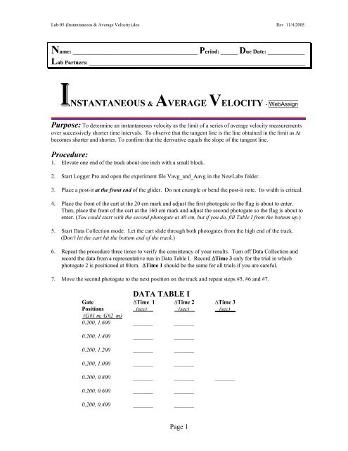
Lab-05-(Instantaneous & Average Velocity).doc Rev 11/4/2005Name: ____________________________________________ Period: ______ Due Date: _____________Lab Partners: ____________________________________________________________________________INSTANTANEOUS & AVERAGE VELOCITY - WebAssignPurpose: To determine an instantaneous velocity as the limit of a series of average velocity measurementsover successively shorter time intervals. To observe that the tangent line is the line obtained in the limit as ∆tbecomes shorter and shorter. To confirm that the derivative equals the slope of the tangent line.Procedure:1. Elevate one end of the track about one inch with a small block.2. Start Logger Pro and open the experiment file Vavg_and_Aavg in the NewLabs folder.3. Place a post-it at the front end of the glider. Do not crumple or bend the post-it note. Its width is critical.4. Place the front of the cart at the 20 cm mark and adjust the first photogate so the flag is about to enter.Then, place the front of the cart at the 160 cm mark and adjust the second photogate so the flag is about toenter. (You could start with the second photogate at 40 cm, but if you do, fill Table I from the bottom up.)5. Start Data Collection mode. Let the cart slide through both photogates from the high end of the track.(Don't let the cart hit the bottom end of the track.)6. Repeat the procedure three times to verify the consistency of your results. Turn off Data Collection andrecord the data from a representative run in Data Table I. Record ∆Time 3 only for the trial in whichphotogate 2 is positioned at 80cm. ∆Time 1 should be the same for all trials if you are careful.7. Move the second photogate to the next position on the track and repeat steps #5, #6 and #7.DATA TABLE IGate ∆Time 1 ∆Time 2 ∆Time 3Positions (sec) (sec) (sec)(G#1 m, G#2 m)0.200, 1.600 _______ _______0.200, 1.400 _______ _______0.200, 1.200 _______ _______0.200, 1.000 _______ _______0.200, 0.800 _______ _______ _______0.200, 0.600 _______ _______0.200, 0.400 _______ _______Page 1

Lab-05-(Instantaneous & Average Velocity).doc Rev 11/4/2005Elapsed Time: The elapsed time is the time interval from the moment the flag enters the first photogateuntil the moment it enters the second photogate. The time interval is the sum, ∆Time 1 + ∆Time 2.Table IIGate t = Elapsed Time = t Gate 2 – t Gate 1 = t Gate 2 – 0Positions (∆Time 1 + ∆Time 2)(G#1 m, G#2 m) (sec)#1 0.200, 1.600 ______________#2 0.200, 1.400 ______________#3 0.200, 1.200 _______ _______#4 0.200, 1.000 _______ _______Analysis:#5 0.200, 0.800 _______ _______ = t r#6 0.200, 0.600 _______ _______#7 0.200, 0.400 _______ _______#8 0.200 _____0.000_____1. Use Graphical Analysis to make a graph of 2 nd gate position vs elapsed time. Call it Graph #1.2. Click at the top of the first data column. Enter time for the name (t for short) and sec for the units. In thesecond column enter position for the name (x for short) and meters for the unit. Enter the elapsed time inthe time column (∆Time 1 + ∆Time 2), and the second gate position in the position column. Graph #1 is aPosition vs Time graph. Add an eighth point at time t = 0.000 sec; the first gate position is x = 0.200 m.3. Click on the graph window. Then click on the Options-GraphOptions menu. Click on Connect Points toturn OFF connecting lines.4. Select Analyze-CurveFit from the menu. The points in Graph #1 should fall on the line described by theposition equation; x = x 0 + v 0 *t + ½ a*t 2 . Click on the Define Function button and edit the box to read0.200 + B*t + 0.5*A*t^2. Click on Try Fit. You should get a parabolic curve that fits the points. ClickOK. Drag the box containing the function away from the curve. (Note: 0.200 m is the starting point for themeasurements, i.e., x 0 . The coefficient of t, B, is the instantaneous initial velocity, v 0 , and the coefficient oft 2 is one-half of the acceleration; thus, A = acceleration = a.) Move the square brackets to the edges.5. Include your name, your class period, the lab number, and the graph name in the text box. Change thecoordinates of the lower left-hand corner of Graph #1 to (–1.000 s , 0.00 m). Set t MAX = 3.0 sec. Setx MAX to 2.0 m. On the Options-GraphOptions menu set Minor Tick Style to “Dashed”. It is also a good ideato deselect (remove the check mark) the “Show Uncertainty” option in the curve fit box’s pop-up menu.6. Print the entire screen, Data, Text and Graph. Then print the Graph by itself. Make sure the printouts are allin landscape mode to make them as large as possible. You might print a couple of copies of the graph alonejust in case you mess up in section 7. Write your name on the graph alone, as there is no text box.Page 2

Lab-05-(Instantaneous & Average Velocity).doc Rev 11/4/20057. You will now attempt to draw the secant lines and the tangent line to a reference point (t r , x r ) on theparabola. The value of t r varies from group to group, but the value of x r , 0.800 meters, is the same for allgroups. Drawing these lines needs to be done carefully, so wait for specific instructions. The graph will be toomessy to read if you make more lines than are needed or if you draw them over too wide a range.Each secant line starts at a data point and then passes through the reference point, whose position is 0.800 m,and then continues for about two inches farther, but NOT to the edge of the graph. Make sure the secant linesonly extend across the parabolic curve at x r = 0.800 m. If you cross the curve at the other point your drawingwill be hard to read and it will be difficult to draw the correct tangent line and measure its slope.With a pencil and a ruler, draw seven straight secant lines each passing between the pairs of position pointsdefined below. The Line connecting each pair of points is called a secant line. If you like color-coding, thendraw the secant lines from the left in one color, and from the right in another. Each secant line should beextended about two inches past the x r = 0.800 m point. Note, all secant lines pass through the point wherex r = 0.800 m. This is the position, for which we hope to find v r , the true instantaneous velocity, at coordinates:(t r sec, x r = 0.800 m) = (__________s, 0.800 m) (Times vary by group, but should be close to t r ≈ 1.7 sec).Make sure your drawing has all the lines passing through this point. (Time is the horizontal axis in this graph.Position is the vertical axis. Think about what you are doing before you start doing it.)The four lines on the left side of the list below come from the upper right section of the graph. These drawnlines come down through the reference point, and are extended down to the left. The three lines on the rightside of the list come from the lower left section of the graph. These drawn lines come up through the referencepoint, and are extended up to the right. The tangent line also goes through the reference point, but it should bebelow the parabola and above all the secant extensions, as shown on the sample graph below. (If you mess upthe graph, reprint it and try again. This needs to be done carefully and correctly.) Make sure the tangent lineextends to the edges of the graph. The points in the list are defined only by their positions. Look to the left sideof the graph, at the vertical axis, when you need to locate one of these points.1.600→0.800 1.400→0.800 1.200→0.800 1.000→0.800 0.200→0.800 0.400→0.800 0.600→0.800The tangent line should be the only drawn-line that extends to the edges of the graph. This sets it apart from theextended secant lines, and makes it easier both to find it and to calculate its slope. Or, use a different color.Notice that the tangent line isconstrained to fall between thesecant line extensions and theparabolic curve. This narrowwindow makes it easier to drawan accurate tangent line. Thetangent line must go through thereference point and both gaps inthe secant line extensions.Below, you will compare theslope of the tangent line to themeasured velocity atx r = 0.800 m, and to the velocitypredicted by the velocityequation at time t r and positionx r = 0.800 m.Page 3

Lab-05-(Instantaneous & Average Velocity).doc Rev 11/4/20058. Calculate the slope of each of the seven, secant lines drawn on Graph #1 (Section 9) plus the slope of thetangent line drawn through the point at (t r , x r = 0.800) (Section 10). The information you need to calculate both∆x and ∆t for the secant lines is contained in Table II. Extensive instructions and sample calculations forcompleting Table III are given below in sections 9 – 12.Table IIIx r→x ∆x = x − x r ∆t = t − t r Slope = ∆x/∆t = average velocity0.800→1.600 +_______________ +_____________ +_____________ m/s0.800→1.400 +_______________ +_____________ +_____________ m/s0.800→1.200 +_______________ +_____________ +_____________ m/s0.800→1.000 +_______________ +_____________ +_____________ m/sManual estimate of the Slope of the tangent lineat x = 0.800 meters (From Graph #1) =v manual = +_____________ m/sCalculus based estimate of the Slope of the tangent line at x = 0.800 meters(From the derivative of the position equation of Graph #1) = v Calculus = +_____________ m/sDirect measurement of the instantaneous velocity at x = 0.800 meters(From the post-it note width and the measured ∆Time 3) = v measured = +_____________ m/s0.800→0.600 −_______________ −_____________ +_____________ m/s0.800→0.400 −_______________ −_____________ +_____________ m/s0.800→0.200 −_______________ −_____________ +_____________ m/s9. The slopes of the secant lines drawn on Graph #1 equal the displacement ∆x = (x − x r ) divided by the timeinterval ∆t = (t − t r ). ∆t is most simply calculated as the difference in elapsed times at the two positions.Adjust the signs accordingly. In the sample graph on the previous page, the elapsed time at 0.800 m was1.628 sec. The elapsed time at 0.200 m was 0.000 sec, therefore, the ∆t between 0.200 m and 0.800 m is0.000 – 1.628 = −1.628 sec. ∆x is (0.200 – 0.800). Thus, the slope of the secant line between 0.200 m and0.800 m = (0.200 – 0.800) / (0 – 1.628) = +0.369 m/s. The average velocity is therefore +0.369 m/s.Here is another example. The elapsed times at 1.600 m and 0.800 m are 2.780 sec and 1.628 sec,respectively. Thus, ∆t = (2.780 – 1.628) = +1.152 sec. ∆x is (1.600 – 0.800). Thus, the slope of the secantline between 1.600 m and 0.800 m = (1.600 – 0.800) / 1.152 = +0.694 m/s = average velocity.Complete section 9 and include the slope of the tangent line in Table III. It should lie between the averagevelocities calculated from the slopes of the secant lines. See section 9 for instructions10. On the graph, use a ruler to draw the tangent to the curve at the point (t r , x r = 0.800 m). Extend the tangentline to the bottom and right edges of the graph. Measure the rise and the run and calculate the slope of thetangent line. This is your manual estimate of the instantaneous velocity, v r , of the cart at (t r , x r = 0.800).Instantaneous Velocity at point (t r , x r = 0.800 m) = Slope of tangent = v manual = _________________ m/sEnter this value in Table III above.Page 4

Lab-05-(Instantaneous & Average Velocity).doc Rev 11/4/200511. The slope of the tangent line (the instantaneous velocity) can also be found by taking the derivative of theposition vs time equation. Graphical Analysis gave you this equation when you found the curve fit forGraph #1. The derivative is a mathematical operation that converts any equation into a new equation thatgives the slope of any line tangent to the original equation. The derivative of the position equation turns outto be the equation we have come to know as the velocity equation.Instantaneous Velocity (at any time t) = d / dt (x) = v = d / dt (0.200 + B t + ½ A t 2 ) = B + A tConsult the equation coefficients on your printed graph: B = v 0 = __________ and A = a = __________As the cart enters the 2 nd photogate at 0.800 m, find the elapsed time t r from your data table. Then find theinstantaneous velocity at that time using the velocity equation derived from the position equation.Instantaneous Velocity at point (t r , x r = 0.800 m) = v Calculus = __________________Enter this calculus-based estimate of the instantaneous velocity, v r , at (t r , x r = 0.800 m) into Table III.The slope of the hand-drawn tangent line on your graph and the calculated derivative give you twoindependent estimates for the instantaneous velocity at (t r , x r = 0.800 m).These two estimates should agree. Do they? ____________ (If not, find your error or see the instructor.)12. You measured ∆Time 3 when the 2 nd photogate was located at x r = 0.800 m, so you also have anopportunity to directly measure the instantaneous velocity at that position. We’ll call this the measuredInstantaneous Velocity at (t r , x r = 0.800 m). It is simply the width of the post-it note divided by ∆Time 3.Width of post-it note = d = ____________ mm = ____________ mInstantaneous Velocity at point (t r , x r = 0.800 m) = v measured = d / ∆Time 3 = ___________ m/sEnter this measured estimate of the instantaneous velocity, v r , at (t r , x r = 0.800 m) into Table III.All three estimates of the instantaneous velocity at point (t r , x r = 0.800 m) should agree. Any differencesshould be very small. Do they agree? ___________ (If not, find your error or see the instructor.)(Note: this measured estimate of v r will probably be a little high, because the cart does travel is little bitfurther than 0.800 m while we make the measurement. That is a bit of error we may just have to live with.)13. To make a quantitative comparison among the three estimates of v r at point (t r , x r = 0.800 m), you willcompute the percent difference between each of them and the mean value of the three estimates. Use themean value as the reference value in the percent difference calculation.First find the mean value = v mean = (v manual + v Calculus + v measured ) / 3 = ________________ m/s%Difference (in v manual ) = 100% | v manual − v mean | / v mean = ____________________ %%Difference (in v Calculus ) = 100% | v Calculus − v mean | / v mean = ____________________ %%Difference (in v measured ) = 100% | v measured − v mean | / v mean = ___________________ %Page 5

Lab-05-(Instantaneous & Average Velocity).doc Rev 11/4/200516. Now compare the y-intercept of the Average Velocity vs Time Interval graph with your three otherestimates of the instantaneous velocity at x = 0.800 m. You will discuss this below. Table III contains threeestimates of the instantaneous velocity, v r , at (t r , x r = 0.800 m). The y-intercept on Graph #2 provides you withyet another estimate of v r at (t r , x r = 0.800 m).b = v Graph #2 = ______________ m/sUse the space below and on the next page to compare your four independent estimates of the instantaneousvelocity, v r , at (t r , x r = 0.800 m), which you have obtained from these exercises. Think beyond your ownpersonal results and describe what general conclusions about instantaneous velocity and its measurement youhave learned through these exercises. Write neatly or type in a word processor and paste your essay into thespaces provided below and on the next page. (The discussion should be both qualitative and quantitative.)Page 7

Lab-05-(Instantaneous & Average Velocity).doc Rev 11/4/2005Page 8