CSE555: Introduction to Pattern Recognition Midterm ... - CEDAR

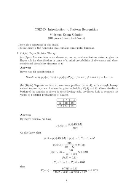
CSE555: Introduction to Pattern RecognitionMidterm Exam Solution(100 points, Closed book/notes)There are 5 questions in this exam.The last page is the Appendix that contains some useful formulas.1. (15pts) Bayes Decision Theory.(a) (5pts) Assume there are c classes w 1 , · · · ,w c , and one feature vector x, give theBayes rule for classification in terms of a priori probabilities of the classes and classconditionalprobability densities of x.Answer:Bayes rule for classification isDecide ω i if p(x|ω i )P(ω i ) > p(x|ω j )P(ω j ) for all j ≠ i and i,j = 1, · · · ,c.(b) (10pts) Suppose we have a two-classes problem (A, ∼ A), with a single binaryvaluedfeature (x, ∼ x). Assume the prior probability P(A) = 0.33. Given the distributionof the samples as shown in the following table, use Bayes Rule to compute thevalues of posterior probabilities of classes.A ∼ Ax 248 167∼ x 82 503Answer:By Bayes formula, we havewe also know thatP(A|x) = p(x|A)P(A)p(x)thusp(x) = p(x|A)P(A) + p(x| ∼ A)P(∼ A) andP(A|x) =p(x|A) = 248248 + 82 ≈ 0.7515167p(x| ∼ A) =167 + 503 ≈ 0.2493P(A) = 0.33P(∼ A) = 1 − P(A) = 0.670.7515 × 0.330.7515 × 0.33 + 0.2493 × 0.67 ≈ 0.59761

Similarly, we haveP(∼ A|x) ≈ 0.4024P(A| ∼ x) ≈ 0.1402P(∼ A| ∼ x) ≈ 0.85982. (25pts) Fisher Linear Discriminant.(a) (5pts) What is the Fisher linear discriminant method?Answer:The Fisher linear discriminant finds a good subspace in which categories are bestseparated in a least-squares sense; other, general classification techniques can thenbe applied in the subspace.(b) Given the 2-d data for two classes:ω 1 = [(1, 1), (1, 2), (1, 4), (2, 1), (3, 1), (3, 3)] andω 2 = [(2, 2), (3, 2), (3, 4), (5, 1), (5, 4), (5, 5)] as shown in the figure:65432100 1 2 3 4 5 6i. (10pts) Determine the optimal projection line in a single dimension.Answer:Let w be the direction of the projection line, then the Fisher linear discriminantmethod finds that the best w is the one for which the criterion functionJ(w) = wt S B ww t S wwis maximum, as followswhereandS i = ∑w = S −1w(m 1 − m 2 )Sw = S 1 + S 2x∈D i(x − m i )(x − m i ) t i = 1, 22

Thus, we first compute the sample means for each class and get[ ] [ ]11 236 62 3m 1 =m 2 =Then we subtract the sample mean from each sample and get[−5−x − m 1 =5 − 5 ]1 7 76 6 6 6 6 6−1 0 2 −1 −1 1thereforeS 1 =S 2 =[−11−x − m 2 =5 − 5 ]7 7 76 6 6 6 6 6−1 −1 1 −2 1 2[ 25+25+25+1+49+49365+0−10−1−7+7[ 121+25+25+49+49+493611+5−5−14+7+145+0−10−1−7+7661 + 0 + 4 + 1 + 1 + 111+5−5−14+7+14661 + 1 + 1 + 4 + 1 + 4and then[ ] 412Sw = S 1 + S 2 = 32 20S −1w = 1 [ ]20 −241 = 1 [ ]20 −2|Sw| −2808 41 =−23 3 3Finally we havew = S −1w =[15− 3202 404− 3 41404 808] [−2−1w (m 1 − m 2 )] [−57= 404− 29808]≈][=][ 2936−1−1 8=[ 53633 1215− 3202 404− 3 41404 808[−0.1411−0.0359ii. (10pts) Show the mapping of the points to the line as well as the Bayes discriminantassuming a suitable distribution.Answer:The samples are mapped by x ′ = w t x and we getw ′ 1 = [−0.1770, −0.2129, −0.2847, −0.3181, −0.4592, −0.5309]w ′ 2 = [−0.3540, −0.4950, −0.5668, −0.7413, −0.8490, −0.8849]and we compute the mean and the standard deviation asµ 1 = 0.3304 σ 1 = 0.1388µ 2 = 0.6485 σ 2 = 0.2106If we assume both p(x|ω 1 ) and p(x|ω 2 ) have a Gaussian distribution, then theBayes decision rule will beDecide ω 1 if p(x|ω i )P(ω 1 ) > p(x|ω 2 )P(ω 2 ); otherwise decide ω 2]]]]3

wherep(x|ω i ) = √ 1 [exp − 1 ( ) ] x − µi 22πσi 2 σ iIf we assume the prior probabilities are equal, i.e. P(ω ′ 1) = P(ω ′ 2) = 0.5, thenthe threshold will be about −0.4933. That is, we decide ω 1 if w t x > −0.4933,otherwise decide ω 2 .3. (20pts) Suppose p(x|w 1 ) and p(x|w 2 ) are defined as follows:p(x|w 1 ) = 1 √2πe − x22 , ∀xp(x|w 2 ) = 1 4, −2 < x < 2(a) (7pts) Find the minimum error classification rule g(x) for this two-class problem,assuming P(w 1 ) = P(w 2 ) = 0.5.Answer:(i) In case of −2 < x < 2, because P(ω 1 ) = P(ω 2 ) = 0.5, we have the discriminantfunction g(x) asg(x) = ln p(x|ω 1)p(x|ω 2 ) = ln √ 4 − x22π 2The Bayes rule for classification will beorDecide ω 1 if g(x) > 0; otherwise decide ω 2Decide ω 1 if − 0.9668 < x < 0.9668; otherwise decide ω 2(ii) In case of x ≥ 2 or x ≤ −2, we always decide ω 1 .(b) (10pts) There is a prior probability of class 1, designated as π ∗ 1, so that if P(w 1 ) >π ∗ 1, the minimum error classification rule is to always decide w 1 regardless of x.Find π ∗ 1.Answer:According to the question, π ∗ 1 will satisfy the following equationp(x|ω 1 )π ∗ 1 = p(x|ω 2 )(1 − π ∗ 1)when x = 2 or x = −2Therefore, we have1√2πe −4 2 π∗1 = 1 4 (1 − π∗ 1)π ∗ 1 ≈ 0.8224(c) (3pts) There is no π ∗ 2 so that if P(w 2 ) > π ∗ 2, we would always decide w 2 . Whynot?Answer:Because p(x|ω 2 ) is only defined for −2 < x < 2, therefore we would always decidew 1 for x ≥ 2 or x ≤ −2, no matter what is the prior probability p(w 2 ).4

4. (20pts) Let samples be drawn by successive, independent selections of a state of naturew i with unknown probability P(w i ). Let z ik = 1 if the state of nature for the kthsample is w i and z ik = 0 otherwise.(a) (7pts) Show thatn∏P(z i1 , · · · ,z in |P(w i )) = P(w i ) z ik(1 − P(w i )) 1−z ikk=1Answer:We are given that{1 if the state of nature for the kz ik =th sample is ω i0 otherwiseThe samples are drawn by successive independent selection of a state of naturew i with probability P(w i ). We have thenandThese two equations can be unified asPr[z ik = 1|P(w i )] = P(w i )Pr[z ik = 0|P(w i )] = 1 − P(w i )P(z ik |P(w i )) = [P(w i )] z ik[1 − P(w i )] 1−z ikBy the independence of the successive selection, we haveP(z i1 , · · · ,z in |P(w i )) ==n∏P(z ik |P(w i ))k=1n∏[P(w i )] z ik[1 − P(w i )] 1−z ikk=1(b) (10pts) Given the equation above, show that the maximum likelihood estimatefor P(w i ) isˆP(w i ) = 1 n∑z iknAnswer:The log-likelihood as a function of P(w i ) isk=1l(P(w i )) = lnP(z i1 , · · · ,z in |P(w i ))[ n]∏= ln [P(w i )] z ik[1 − P(w i )] 1−z ikk=1n∑= [z ik ln P(w i ) + (1 − z ik ) ln(1 − P(w i ))]k=1Therefore, the maximum-likelihood values for the P(w i ) must satisfy∇ P(wi )l(P(w i )) = 1P(w i )n∑z ik −k=1511 − P(w i )n∑(1 − z ik ) = 0k=1

We solve this equation and findwhich can be rewritten asThe final solution is then(1 − ˆP(wn∑i )) z ik = ˆP(wn∑i ) (1 − z ik )k=1k=1n∑z ik = ˆP(wn∑i ) z ik + n ˆP(w i ) − ˆP(wn∑i ) z ikk=1k=1k=1ˆP(w i ) = 1 n∑z iknk=1(c) (3pts) Interpret the meaning of your result in words.Answer:In this question, we apply the maximum-likelihood method to estimate the priorprobability. From the result in part (b), it can be observed that the estimate ofthe probability of category w i is merely the probability of obtaining its indicatoryvalue in the training data, just as we would expect.5. (20pts) Consider an HMM with an explicit absorber state w 0 and unique null visiblesymbol v 0 with the following transition probabilities a ij and symbol probabilities b jk(where the matrix indexes begin at 0):a ij =⎛⎜⎝1 0 00.2 0.3 0.50.4 0.5 0.1⎞⎟⎠ b jk =⎛⎜⎝1 0 00 0.7 0.30 0.4 0.6⎞⎟⎠(a) (7pts) Give a graph representation of this Hidden Markov Model.Answer:0.3ω0.210.3 0.7v2v110.50.5ω01v00.40.4v 1ω20.6v20.16

(b) (10pts) Suppose the initial hidden state at t = 0 is w 1 . Starting from t = 1, whatis the probability it generates the particular sequence V 3 = {v 2 ,v 1 ,v 0 }?Answer:The probability of observing the sequence V 3 is 0.03678. See the figure below forthe details.vv2 10vW0W1W20 0.036781*.3*.3 *.3*.70 0.30.09 0.1239*.5*.6*.5*.7 *.5*.4*.4*1*.1*.40.03*.2*1t=0 1 2 3(c) (3pts) Given the above sequence V 3 , what is the most probable sequence of hiddenstates?Answer:From the figure above and by using the decoding algorithm, one can observe thatthe most probable sequence of hidden states is {w 1 ,w 2 ,w 1 ,w 0 }.7

Appendix: Useful formulas.• For a 2 × 2 matrix,A =[a bc dthe matrix inverse isA −1 = 1 [ ]d −b=|A| −c a]1ad − bc[d −b−c a]• The scatter matrices S i are defined asS i = ∑x∈D i(x − m i )(x − m i ) twhere m i is the d-dimensional sample mean.The within-class scatter matrix is defined asS W = S 1 + S 2The between-class scatter matrix is defined asS B = (m 1 − m 2 )(m 1 − m 2 ) tThe solution for the w that optimizes J(w) = wt S B ww t S W w isw = S −1W (m 1 − m 2 )8