Null Controllability for Degenerate Parabolic Operators
Null Controllability for Degenerate Parabolic Operators
Null Controllability for Degenerate Parabolic Operators

You also want an ePaper? Increase the reach of your titles
YUMPU automatically turns print PDFs into web optimized ePapers that Google loves.
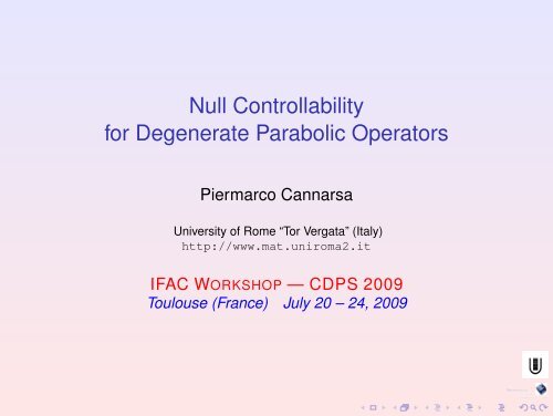
<strong>Null</strong> <strong>Controllability</strong><strong>for</strong> <strong>Degenerate</strong> <strong>Parabolic</strong> <strong>Operators</strong>Piermarco CannarsaUniversity of Rome “Tor Vergata” (Italy)http://www.mat.uniroma2.itIFAC WORKSHOP — CDPS 2009Toulouse (France) July 20 – 24, 2009
degenerate parabolic operatorsO ⊂ R nwherewithbounded⎧⎪⎨ u t − Lu = f in O×]0, T [u(x, 0) = u 0 (x) x ∈ O⎪⎩(possibly) + b. c. on ∂O×]0, T [⎧⎪⎨ div(A(x)∇u) + lower order tmsLu = or⎪⎩Tr [A(x)∇ 2 u] + lower order tmsA(x) > 0 in O but A(x) ≥ 0 on ∂O
degenerate parabolic operatorsO ⊂ R nwherewithbounded⎧⎪⎨ u t − Lu = f in O×]0, T [u(x, 0) = u 0 (x) x ∈ O⎪⎩(possibly) + b. c. on ∂O×]0, T [⎧⎪⎨ div(A(x)∇u) + lower order tmsLu = or⎪⎩Tr [A(x)∇ 2 u] + lower order tmsA(x) > 0 in O but A(x) ≥ 0 on ∂O
Outline1 Examples of degenerate parabolic problems2 <strong>Null</strong> controllability <strong>for</strong> degenerate parabolic operatorsintroduction to null controllabilityone dimensional case3 Higher dimensional problems
Outline1 Examples of degenerate parabolic problems2 <strong>Null</strong> controllability <strong>for</strong> degenerate parabolic operatorsintroduction to null controllabilityone dimensional case3 Higher dimensional problems
examples of degenerate problems• laminar flow on flat plates(Crocco type equations)• mathematical finance(Black & Scholes type equations)• climate models(Budyko-Sellers)• population genetics(Wrigth-Fisher, Fleming-Viot diffusion processes)• domain invariance <strong>for</strong> stochastic flow(Friedman & Pinsky, Da Prato & Frankowska)
examples of degenerate problems• laminar flow on flat plates(Crocco type equations)• mathematical finance(Black & Scholes type equations)• climate models(Budyko-Sellers)• population genetics(Wrigth-Fisher, Fleming-Viot diffusion processes)• domain invariance <strong>for</strong> stochastic flow(Friedman & Pinsky, Da Prato & Frankowska)
examples of degenerate problems• laminar flow on flat plates(Crocco type equations)• mathematical finance(Black & Scholes type equations)• climate models(Budyko-Sellers)• population genetics(Wrigth-Fisher, Fleming-Viot diffusion processes)• domain invariance <strong>for</strong> stochastic flow(Friedman & Pinsky, Da Prato & Frankowska)
examples of degenerate problems• laminar flow on flat plates(Crocco type equations)• mathematical finance(Black & Scholes type equations)• climate models(Budyko-Sellers)• population genetics(Wrigth-Fisher, Fleming-Viot diffusion processes)• domain invariance <strong>for</strong> stochastic flow(Friedman & Pinsky, Da Prato & Frankowska)
examples of degenerate problems• laminar flow on flat plates(Crocco type equations)• mathematical finance(Black & Scholes type equations)• climate models(Budyko-Sellers)• population genetics(Wrigth-Fisher, Fleming-Viot diffusion processes)• domain invariance <strong>for</strong> stochastic flow(Friedman & Pinsky, Da Prato & Frankowska)
examples of degenerate problems• laminar flow on flat plates(Crocco type equations)• mathematical finance(Black & Scholes type equations)• climate models(Budyko-Sellers)• population genetics(Wrigth-Fisher, Fleming-Viot diffusion processes)• domain invariance <strong>for</strong> stochastic flow(Friedman & Pinsky, Da Prato & Frankowska)
{ut − ( (1 − x 2 )u x)(1 − x 2 )u x|x=±1 = 0xa climate model= f (x) g(x, u) − h(u) x ∈ (−1, 1)Budyko-Sellers (1969)effect of solar radiation on climate✬✩x = sin α α✫✪• u(t, x) = sea-level zonally averaged temperature• f (x) = solar input• g(x, u) = co-albedo• h(u) = outgoing infrared radiation
{ut − ( (1 − x 2 )u x)(1 − x 2 )u x|x=±1 = 0xa climate model= f (x) g(x, u) − h(u) x ∈ (−1, 1)Budyko-Sellers (1969)effect of solar radiation on climate✬✩x = sin α α✫✪• u(t, x) = sea-level zonally averaged temperature• f (x) = solar input• g(x, u) = co-albedo• h(u) = outgoing infrared radiation
{ut − ( (1 − x 2 )u x)(1 − x 2 )u x|x=±1 = 0xa climate model= f (x) g(x, u) − h(u) x ∈ (−1, 1)Budyko-Sellers (1969)effect of solar radiation on climate✬✩x = sin α α✫✪• u(t, x) = sea-level zonally averaged temperature• f (x) = solar input• g(x, u) = co-albedo• h(u) = outgoing infrared radiation
{ut − ( (1 − x 2 )u x)(1 − x 2 )u x|x=±1 = 0xa climate model= f (x) g(x, u) − h(u) x ∈ (−1, 1)Budyko-Sellers (1969)effect of solar radiation on climate✬✩x = sin α α✫✪• u(t, x) = sea-level zonally averaged temperature• f (x) = solar input• g(x, u) = co-albedo• h(u) = outgoing infrared radiation
Fleming-Viot diffusion processevolution of genetic types in a populationu t − Tr ( A(x)∇ 2 u ) = · · ·in O = {(x 1 , x 2 ) ∈ R 2 | x i ∈]0, 1[ , x 1 + x 2 ≤ 1}❅❅❅❅O ❅❅❅withA(x 1 , x 2 ) =(x1 (1 − x 1 ) −x 1 x 2−x 1 x 2 x 2 (1 − x 2 ))notice det A(x 1 , x 2 ) = x 1 x 2 (1 − x 1 − x 2 ) = 0 on ∂O
Fleming-Viot diffusion processevolution of genetic types in a populationu t − Tr ( A(x)∇ 2 u ) = · · ·in O = {(x 1 , x 2 ) ∈ R 2 | x i ∈]0, 1[ , x 1 + x 2 ≤ 1}❅❅❅❅O ❅❅❅withA(x 1 , x 2 ) =(x1 (1 − x 1 ) −x 1 x 2−x 1 x 2 x 2 (1 − x 2 ))notice det A(x 1 , x 2 ) = x 1 x 2 (1 − x 1 − x 2 ) = 0 on ∂O
Fleming-Viot diffusion processevolution of genetic types in a populationu t − Tr ( A(x)∇ 2 u ) = · · ·in O = {(x 1 , x 2 ) ∈ R 2 | x i ∈]0, 1[ , x 1 + x 2 ≤ 1}❅❅❅❅O ❅❅❅withA(x 1 , x 2 ) =(x1 (1 − x 1 ) −x 1 x 2−x 1 x 2 x 2 (1 − x 2 ))notice det A(x 1 , x 2 ) = x 1 x 2 (1 − x 1 − x 2 ) = 0 on ∂O
Fleming-Viot diffusion processevolution of genetic types in a populationu t − Tr ( A(x)∇ 2 u ) = · · ·in O = {(x 1 , x 2 ) ∈ R 2 | x i ∈]0, 1[ , x 1 + x 2 ≤ 1}❅❅❅❅O ❅❅❅withA(x 1 , x 2 ) =(x1 (1 − x 1 ) −x 1 x 2−x 1 x 2 x 2 (1 − x 2 ))notice det A(x 1 , x 2 ) = x 1 x 2 (1 − x 1 − x 2 ) = 0 on ∂O
Fleming-Viot diffusion processevolution of genetic types in a populationu t − Tr ( A(x)∇ 2 u ) = · · ·in O = {(x 1 , x 2 ) ∈ R 2 | x i ∈]0, 1[ , x 1 + x 2 ≤ 1}❅❅❅❅O ❅❅❅withA(x 1 , x 2 ) =(x1 (1 − x 1 ) −x 1 x 2−x 1 x 2 x 2 (1 − x 2 ))notice det A(x 1 , x 2 ) = x 1 x 2 (1 − x 1 − x 2 ) = 0 on ∂O
• X(·, x)invariant sets <strong>for</strong> stochastic flowsunique solution{dX(t) = b(X(t))dt + σ(X(t)) dW (t) t ≥ 0X(0) = x ∈ R n• b : R n → R n , σ : R n → L(R n ; R m ) Lipschitz• W (t) m-dimensional Brownian (Ω, F, {F t } t , P)• K ⊂ R n invariantx ∈ K =⇒ X(t, x) ∈ K P − a.s. ∀t ≥ 0✬ K x✩✫✪
• X(·, x)invariant sets <strong>for</strong> stochastic flowsunique solution{dX(t) = b(X(t))dt + σ(X(t)) dW (t) t ≥ 0X(0) = x ∈ R n• b : R n → R n , σ : R n → L(R n ; R m ) Lipschitz• W (t) m-dimensional Brownian (Ω, F, {F t } t , P)• K ⊂ R n invariantx ∈ K =⇒ X(t, x) ∈ K P − a.s. ∀t ≥ 0✬ K x✩✫✪
• X(·, x)invariant sets <strong>for</strong> stochastic flowsunique solution{dX(t) = b(X(t))dt + σ(X(t)) dW (t) t ≥ 0X(0) = x ∈ R n• b : R n → R n , σ : R n → L(R n ; R m ) Lipschitz• W (t) m-dimensional Brownian (Ω, F, {F t } t , P)• K ⊂ R n invariantx ∈ K =⇒ X(t, x) ∈ K P − a.s. ∀t ≥ 0✬ K x✩✫✪
two invariance problemsProblemgiven O ⊂ R n open (∂O = Γ) to study invariance of• closed domain• open domainOOKolmogorov operator{D(L 0 ) = { ϕ ∈ C(O) ∣ ∣ ϕ ∈ H 2 loc (O) , L 0ϕ ∈ C(O) }L 0 ϕ(x) := 1 2 Tr [A(x)∇2 ϕ(x)] + 〈b(x), ∇ϕ(x)〉x ∈ Owhere A(x) = σ(x)σ ∗ (x) ≥ 0oriented{distance from Γ❅d Γdist(x, Γ) if x ∈ Od Γ (x) =Γ ❅−dist(x, Γ) if x ∈ O c ❅ O ❅
two invariance problemsProblemgiven O ⊂ R n open (∂O = Γ) to study invariance of• closed domain• open domainOOKolmogorov operator{D(L 0 ) = { ϕ ∈ C(O) ∣ ∣ ϕ ∈ H 2 loc (O) , L 0ϕ ∈ C(O) }L 0 ϕ(x) := 1 2 Tr [A(x)∇2 ϕ(x)] + 〈b(x), ∇ϕ(x)〉x ∈ Owhere A(x) = σ(x)σ ∗ (x) ≥ 0oriented{distance from Γ❅d Γdist(x, Γ) if x ∈ Od Γ (x) =Γ ❅−dist(x, Γ) if x ∈ O c ❅ O ❅
two invariance problemsProblemgiven O ⊂ R n open (∂O = Γ) to study invariance of• closed domain• open domainOOKolmogorov operator{D(L 0 ) = { ϕ ∈ C(O) ∣ ∣ ϕ ∈ H 2 loc (O) , L 0ϕ ∈ C(O) }L 0 ϕ(x) := 1 2 Tr [A(x)∇2 ϕ(x)] + 〈b(x), ∇ϕ(x)〉x ∈ Owhere A(x) = σ(x)σ ∗ (x) ≥ 0oriented{distance from Γ❅d Γdist(x, Γ) if x ∈ Od Γ (x) =Γ ❅−dist(x, Γ) if x ∈ O c ❅ O ❅
two invariance problemsProblemgiven O ⊂ R n open (∂O = Γ) to study invariance of• closed domain• open domainOOKolmogorov operator{D(L 0 ) = { ϕ ∈ C(O) ∣ ∣ ϕ ∈ H 2 loc (O) , L 0ϕ ∈ C(O) }L 0 ϕ(x) := 1 2 Tr [A(x)∇2 ϕ(x)] + 〈b(x), ∇ϕ(x)〉x ∈ Owhere A(x) = σ(x)σ ∗ (x) ≥ 0oriented{distance from Γ❅d Γdist(x, Γ) if x ∈ Od Γ (x) =Γ ❅−dist(x, Γ) if x ∈ O c ❅ O ❅
two invariance problemsProblemgiven O ⊂ R n open (∂O = Γ) to study invariance of• closed domain• open domainOOKolmogorov operator{D(L 0 ) = { ϕ ∈ C(O) ∣ ∣ ϕ ∈ H 2 loc (O) , L 0ϕ ∈ C(O) }L 0 ϕ(x) := 1 2 Tr [A(x)∇2 ϕ(x)] + 〈b(x), ∇ϕ(x)〉x ∈ Owhere A(x) = σ(x)σ ∗ (x) ≥ 0oriented{distance from Γ❅d Γdist(x, Γ) if x ∈ Od Γ (x) =Γ ❅−dist(x, Γ) if x ∈ O c ❅ O ❅
two invariance problemsProblemgiven O ⊂ R n open (∂O = Γ) to study invariance of• closed domain• open domainOOKolmogorov operator{D(L 0 ) = { ϕ ∈ C(O) ∣ ∣ ϕ ∈ H 2 loc (O) , L 0ϕ ∈ C(O) }L 0 ϕ(x) := 1 2 Tr [A(x)∇2 ϕ(x)] + 〈b(x), ∇ϕ(x)〉x ∈ Owhere A(x) = σ(x)σ ∗ (x) ≥ 0oriented{distance from Γ❅d Γdist(x, Γ) if x ∈ Od Γ (x) =Γ ❅−dist(x, Γ) if x ∈ O c ❅ O ❅
Theoremconditions <strong>for</strong> invariance(a) ⇐⇒ (b) ⇐⇒ (c)(a) O invariant{(i) L0 d Γ (x) ≥ 0(b) ∀x ∈ Γ(ii) 〈A(x)∇d Γ (x), ∇d Γ (x)〉 = 0(c) O invariantref Friedman & Pinsky (1975)Da Prato & Frankowska (2004)C & Da Prato & Frankowska (2009)stochastic viability . . .invariance =⇒ L 0 degenerate on Γ
Theoremconditions <strong>for</strong> invariance(a) ⇐⇒ (b) ⇐⇒ (c)(a) O invariant{(i) L0 d Γ (x) ≥ 0(b) ∀x ∈ Γ(ii) 〈A(x)∇d Γ (x), ∇d Γ (x)〉 = 0(c) O invariantref Friedman & Pinsky (1975)Da Prato & Frankowska (2004)C & Da Prato & Frankowska (2009)stochastic viability . . .invariance =⇒ L 0 degenerate on Γ
Theoremconditions <strong>for</strong> invariance(a) ⇐⇒ (b) ⇐⇒ (c)(a) O invariant{(i) L0 d Γ (x) ≥ 0(b) ∀x ∈ Γ(ii) 〈A(x)∇d Γ (x), ∇d Γ (x)〉 = 0(c) O invariantref Friedman & Pinsky (1975)Da Prato & Frankowska (2004)C & Da Prato & Frankowska (2009)stochastic viability . . .invariance =⇒ L 0 degenerate on Γ
Theoremconditions <strong>for</strong> invariance(a) ⇐⇒ (b) ⇐⇒ (c)(a) O invariant{(i) L0 d Γ (x) ≥ 0(b) ∀x ∈ Γ(ii) 〈A(x)∇d Γ (x), ∇d Γ (x)〉 = 0(c) O invariantref Friedman & Pinsky (1975)Da Prato & Frankowska (2004)C & Da Prato & Frankowska (2009)stochastic viability . . .invariance =⇒ L 0 degenerate on Γ
Theoremconditions <strong>for</strong> invariance(a) ⇐⇒ (b) ⇐⇒ (c)(a) O invariant{(i) L0 d Γ (x) ≥ 0(b) ∀x ∈ Γ(ii) 〈A(x)∇d Γ (x), ∇d Γ (x)〉 = 0(c) O invariantref Friedman & Pinsky (1975)Da Prato & Frankowska (2004)C & Da Prato & Frankowska (2009)stochastic viability . . .invariance =⇒ L 0 degenerate on Γ
Theoremconditions <strong>for</strong> invariance(a) ⇐⇒ (b) ⇐⇒ (c)(a) O invariant{(i) L0 d Γ (x) ≥ 0(b) ∀x ∈ Γ(ii) 〈A(x)∇d Γ (x), ∇d Γ (x)〉 = 0(c) O invariantref Friedman & Pinsky (1975)Da Prato & Frankowska (2004)C & Da Prato & Frankowska (2009)stochastic viability . . .invariance =⇒ L 0 degenerate on Γ
Outline1 Examples of degenerate parabolic problems2 <strong>Null</strong> controllability <strong>for</strong> degenerate parabolic operatorsintroduction to null controllabilityone dimensional case3 Higher dimensional problems
controlled parabolic equationsω ⊂⊂ O T > 0⎧⎪⎨ u t − div(A(x)∇u) = χ ω (x)f (t, x) in Q T := O×]0, T [u f → u(x, 0) = u 0 (x)x ∈ O⎪⎩(possibly + boundary conditions)• f controlχ ω characteristic function of ω• A(x) = ( a ij (x) ) ni,j=1• a ij = a ji ∈ C(O) ∩ C 1 (O)• positive definite in O (not in O)✬✩✓✏ω✒✑✫O✪
the null controllability problemwant to study null-controllability in time T > 0∀u 0 ∈ L 2 (O) ∃f ∈ L 2 (Q T ) :{u f (·, T ) ≡ 0∫Q T|f | 2 ≤ C T∫O |u 0| 2uni<strong>for</strong>mly parabolic equations∃ m > 0 : A(x) ≥ m I n =⇒ null-controllability ∀ T > 0• Fattorini and Russell (1971), Russell (1978)• Lebeau and Robbiano (1995)• Fursikov and Emanouilov (1996)• Tataru (1997)
the null controllability problemwant to study null-controllability in time T > 0∀u 0 ∈ L 2 (O) ∃f ∈ L 2 (Q T ) :{u f (·, T ) ≡ 0∫Q T|f | 2 ≤ C T∫O |u 0| 2uni<strong>for</strong>mly parabolic equations∃ m > 0 : A(x) ≥ m I n =⇒ null-controllability ∀ T > 0• Fattorini and Russell (1971), Russell (1978)• Lebeau and Robbiano (1995)• Fursikov and Emanouilov (1996)• Tataru (1997)
the null controllability problemwant to study null-controllability in time T > 0∀u 0 ∈ L 2 (O) ∃f ∈ L 2 (Q T ) :{u f (·, T ) ≡ 0∫Q T|f | 2 ≤ C T∫O |u 0| 2uni<strong>for</strong>mly parabolic equations∃ m > 0 : A(x) ≥ m I n =⇒ null-controllability ∀ T > 0• Fattorini and Russell (1971), Russell (1978)• Lebeau and Robbiano (1995)• Fursikov and Emanouilov (1996)• Tataru (1997)
oadmap to null controllability• show equivalence with observability inequality{adjoint v t +div(A(x)∇v) = 0 in Q Tproblem v = 0 on Γ×]0, T [=⇒∫O∫ T ∫v 2 (x, 0) dx ≤ C T• prove observability by Carleman’s estimates > 0 large∫∫Q Ts 3 θ 3 (t)v 2} {{ }e 2sφ(x,t) dxdt ≤ C+sθ(t)|Dv| 2 +···0ωv 2 (x, t) dxdt∫ T0∫ωv 2 dxdtφ(x, t) = θ(t) [ e rψ(x) − e 2r‖ψ‖∞] any Dψ(x) ≠ 0 in O \ ω
oadmap to null controllability• show equivalence with observability inequality{adjoint v t +div(A(x)∇v) = 0 in Q Tproblem v = 0 on Γ×]0, T [=⇒∫O∫ T ∫v 2 (x, 0) dx ≤ C T• prove observability by Carleman’s estimates > 0 large∫∫Q Ts 3 θ 3 (t)v 2} {{ }e 2sφ(x,t) dxdt ≤ C+sθ(t)|Dv| 2 +···0ωv 2 (x, t) dxdt∫ T0∫ωv 2 dxdtφ(x, t) = θ(t) [ e rψ(x) − e 2r‖ψ‖∞] any Dψ(x) ≠ 0 in O \ ω
oadmap to null controllability• show equivalence with observability inequality{adjoint v t +div(A(x)∇v) = 0 in Q Tproblem v = 0 on Γ×]0, T [=⇒∫O∫ T ∫v 2 (x, 0) dx ≤ C T• prove observability by Carleman’s estimates > 0 large∫∫Q Ts 3 θ 3 (t)v 2} {{ }e 2sφ(x,t) dxdt ≤ C+sθ(t)|Dv| 2 +···0ωv 2 (x, t) dxdt∫ T0∫ωv 2 dxdtφ(x, t) = θ(t) [ e rψ(x) − e 2r‖ψ‖∞] any Dψ(x) ≠ 0 in O \ ω
difficulties in degenerate case<strong>for</strong> degenerate parabolic equations:• observability (⇒ null controllability) may fail(<strong>for</strong> violent degeneracies)• φ in Carleman must be adapted to degeneracy• Carleman’s estimate up to higher order terms• Hardy’s inequality essential α ≠ 1∫∫d α−2Γw 2 dx ≤ C dΓ α |∇w|2 dxOO
difficulties in degenerate case<strong>for</strong> degenerate parabolic equations:• observability (⇒ null controllability) may fail(<strong>for</strong> violent degeneracies)• φ in Carleman must be adapted to degeneracy• Carleman’s estimate up to higher order terms• Hardy’s inequality essential α ≠ 1∫∫d α−2Γw 2 dx ≤ C dΓ α |∇w|2 dxOO
difficulties in degenerate case<strong>for</strong> degenerate parabolic equations:• observability (⇒ null controllability) may fail(<strong>for</strong> violent degeneracies)• φ in Carleman must be adapted to degeneracy• Carleman’s estimate up to higher order terms• Hardy’s inequality essential α ≠ 1∫∫d α−2Γw 2 dx ≤ C dΓ α |∇w|2 dxOO
difficulties in degenerate case<strong>for</strong> degenerate parabolic equations:• observability (⇒ null controllability) may fail(<strong>for</strong> violent degeneracies)• φ in Carleman must be adapted to degeneracy• Carleman’s estimate up to higher order terms• Hardy’s inequality essential α ≠ 1∫∫d α−2Γw 2 dx ≤ C dΓ α |∇w|2 dxOO
difficulties in degenerate case<strong>for</strong> degenerate parabolic equations:• observability (⇒ null controllability) may fail(<strong>for</strong> violent degeneracies)• φ in Carleman must be adapted to degeneracy• Carleman’s estimate up to higher order terms• Hardy’s inequality essential α ≠ 1∫∫d α−2Γw 2 dx ≤ C dΓ α |∇w|2 dxOO
Outline1 Examples of degenerate parabolic problems2 <strong>Null</strong> controllability <strong>for</strong> degenerate parabolic operatorsintroduction to null controllabilityone dimensional case3 Higher dimensional problems
one space dimensiona ∈ C([0, 1]) ∩ C 1 (]0, 1]) and a > 0 on ]0, 1]{u t − ( a(x)u x)x = f in Q T =]0, 1[×]0, T [u(x, 0) = u 0 (x)u 0 ∈ L 2 (0, 1) , f ∈ L 2 (Q T )Campiti, Metafune, Pallara (1998)weakly degenerate case: 1/a ∈ L 1 (0, 1)H 1 a(0, 1) ={u ∈ L 2 (0, 1) ∣ ∣∫ 1strongly degenerate case: 1/a /∈ L 1 (0, 1)H 1 a(0, 1) =0{u ∈ L 2 (0, 1) ∣ ∣}aux 2 dx < ∞ & u(0) = 0 = u(1)∫ 10}aux 2 dx < ∞ & u(1) = 0
one space dimensiona ∈ C([0, 1]) ∩ C 1 (]0, 1]) and a > 0 on ]0, 1]{u t − ( a(x)u x)x = f in Q T =]0, 1[×]0, T [u(x, 0) = u 0 (x)u 0 ∈ L 2 (0, 1) , f ∈ L 2 (Q T )Campiti, Metafune, Pallara (1998)weakly degenerate case: 1/a ∈ L 1 (0, 1)H 1 a(0, 1) ={u ∈ L 2 (0, 1) ∣ ∣∫ 1strongly degenerate case: 1/a /∈ L 1 (0, 1)H 1 a(0, 1) =0{u ∈ L 2 (0, 1) ∣ ∣}aux 2 dx < ∞ & u(0) = 0 = u(1)∫ 10}aux 2 dx < ∞ & u(1) = 0
one space dimensiona ∈ C([0, 1]) ∩ C 1 (]0, 1]) and a > 0 on ]0, 1]{u t − ( a(x)u x)x = f in Q T =]0, 1[×]0, T [u(x, 0) = u 0 (x)u 0 ∈ L 2 (0, 1) , f ∈ L 2 (Q T )Campiti, Metafune, Pallara (1998)weakly degenerate case: 1/a ∈ L 1 (0, 1)H 1 a(0, 1) ={u ∈ L 2 (0, 1) ∣ ∣∫ 1strongly degenerate case: 1/a /∈ L 1 (0, 1)H 1 a(0, 1) =0{u ∈ L 2 (0, 1) ∣ ∣}aux 2 dx < ∞ & u(0) = 0 = u(1)∫ 10}aux 2 dx < ∞ & u(1) = 0
one space dimensiona ∈ C([0, 1]) ∩ C 1 (]0, 1]) and a > 0 on ]0, 1]{u t − ( a(x)u x)x = f in Q T =]0, 1[×]0, T [u(x, 0) = u 0 (x)u 0 ∈ L 2 (0, 1) , f ∈ L 2 (Q T )Campiti, Metafune, Pallara (1998)weakly degenerate case: 1/a ∈ L 1 (0, 1)H 1 a(0, 1) ={u ∈ L 2 (0, 1) ∣ ∣∫ 1strongly degenerate case: 1/a /∈ L 1 (0, 1)H 1 a(0, 1) =0{u ∈ L 2 (0, 1) ∣ ∣}aux 2 dx < ∞ & u(0) = 0 = u(1)∫ 10}aux 2 dx < ∞ & u(1) = 0
well-posednessin both cases{D(A) ={u ∈ H1a (0, 1) ∣ ∣ au x ∈ H 1 (0, 1)}Au = ( au x)xgenerates analytic semigroup in L 2 (0, 1)(u• t − `a(x)u x´= f in Q xT =]0, 1[×]0, T [u(x, 0) = u 0 (x)unique solution u ∈ C(0, T ; L 2 (0, 1)) ∩ L 2 (0, T ; Ha(0, 1 1))• maximal regularityu 0 ∈ H 1 a(0, 1) =⇒ u ∈ H 1 (0, T ; L 2 (0, 1))∩L 2 (0, T ; D(A))• strongly degenerate caseu ∈ D(A) =⇒ au x(x→0)−→ 0
well-posednessin both cases{D(A) ={u ∈ H1a (0, 1) ∣ ∣ au x ∈ H 1 (0, 1)}Au = ( au x)xgenerates analytic semigroup in L 2 (0, 1)(u• t − `a(x)u x´= f in Q xT =]0, 1[×]0, T [u(x, 0) = u 0 (x)unique solution u ∈ C(0, T ; L 2 (0, 1)) ∩ L 2 (0, T ; Ha(0, 1 1))• maximal regularityu 0 ∈ H 1 a(0, 1) =⇒ u ∈ H 1 (0, T ; L 2 (0, 1))∩L 2 (0, T ; D(A))• strongly degenerate caseu ∈ D(A) =⇒ au x(x→0)−→ 0
well-posednessin both cases{D(A) ={u ∈ H1a (0, 1) ∣ ∣ au x ∈ H 1 (0, 1)}Au = ( au x)xgenerates analytic semigroup in L 2 (0, 1)(u• t − `a(x)u x´= f in Q xT =]0, 1[×]0, T [u(x, 0) = u 0 (x)unique solution u ∈ C(0, T ; L 2 (0, 1)) ∩ L 2 (0, T ; Ha(0, 1 1))• maximal regularityu 0 ∈ H 1 a(0, 1) =⇒ u ∈ H 1 (0, T ; L 2 (0, 1))∩L 2 (0, T ; D(A))• strongly degenerate caseu ∈ D(A) =⇒ au x(x→0)−→ 0
well-posednessin both cases{D(A) ={u ∈ H1a (0, 1) ∣ ∣ au x ∈ H 1 (0, 1)}Au = ( au x)xgenerates analytic semigroup in L 2 (0, 1)(u• t − `a(x)u x´= f in Q xT =]0, 1[×]0, T [u(x, 0) = u 0 (x)unique solution u ∈ C(0, T ; L 2 (0, 1)) ∩ L 2 (0, T ; Ha(0, 1 1))• maximal regularityu 0 ∈ H 1 a(0, 1) =⇒ u ∈ H 1 (0, T ; L 2 (0, 1))∩L 2 (0, T ; D(A))• strongly degenerate caseu ∈ D(A) =⇒ au x(x→0)−→ 0
well-posednessin both cases{D(A) ={u ∈ H1a (0, 1) ∣ ∣ au x ∈ H 1 (0, 1)}Au = ( au x)xgenerates analytic semigroup in L 2 (0, 1)(u• t − `a(x)u x´= f in Q xT =]0, 1[×]0, T [u(x, 0) = u 0 (x)unique solution u ∈ C(0, T ; L 2 (0, 1)) ∩ L 2 (0, T ; Ha(0, 1 1))• maximal regularityu 0 ∈ H 1 a(0, 1) =⇒ u ∈ H 1 (0, T ; L 2 (0, 1))∩L 2 (0, T ; D(A))• strongly degenerate caseu ∈ D(A) =⇒ au x(x→0)−→ 0
the simplest exampleω =]a, b[⊂⊂]0, 1[ a(x) = x α (α > 0)u t − ( x α u x)x = χ ωf , u(0, x) = u 0 (x)C & Martinez & Vancostenoble (2008)⎧⎪⎨ false α ≥ 2 (→{regional null controllability)n. c.any b.c. 0 ≤ α < 1 weak⎪⎩ true 0 ≤ α < 2Neumann b.c. 1 ≤ α < 2 strongTregional 0 ω 1Figure: regional null controllability
the simplest exampleω =]a, b[⊂⊂]0, 1[ a(x) = x α (α > 0)u t − ( x α u x)x = χ ωf , u(0, x) = u 0 (x)C & Martinez & Vancostenoble (2008)⎧⎪⎨ false α ≥ 2 (→{regional null controllability)n. c.any b.c. 0 ≤ α < 1 weak⎪⎩ true 0 ≤ α < 2Neumann b.c. 1 ≤ α < 2 strongTregional 0 ω 1Figure: regional null controllability
why null controllability fails <strong>for</strong> α ≥ 2• classical change of variable (Courant-Hilbert)y(x) =∫ 1xdss α/2 U(y(x), t) = x −α/4 u(x, t)trans<strong>for</strong>ms equation into˜ω =]˜b, ã[ boundedU t − U yy + V α (y)U = χ eω F0 < y < ∞V α (y) = α 2( 34 α − 1) 1[2−(2−α)y] 2 bounded <strong>for</strong> α ≥ 2• Escauriaza, Seregin, Sverak (2003, 2004)U(·, T ) = 0 ⇐⇒ spt ( U(·, 0) ) ⊂ [0, ã[• u t − ( x α u x)x = χ ωf{no [0, 1]yes if spt(u 0 ) ⊂]a, 1]
why null controllability fails <strong>for</strong> α ≥ 2• classical change of variable (Courant-Hilbert)y(x) =∫ 1xdss α/2 U(y(x), t) = x −α/4 u(x, t)trans<strong>for</strong>ms equation into˜ω =]˜b, ã[ boundedU t − U yy + V α (y)U = χ eω F0 < y < ∞V α (y) = α 2( 34 α − 1) 1[2−(2−α)y] 2 bounded <strong>for</strong> α ≥ 2• Escauriaza, Seregin, Sverak (2003, 2004)U(·, T ) = 0 ⇐⇒ spt ( U(·, 0) ) ⊂ [0, ã[• u t − ( x α u x)x = χ ωf{no [0, 1]yes if spt(u 0 ) ⊂]a, 1]
why null controllability fails <strong>for</strong> α ≥ 2• classical change of variable (Courant-Hilbert)y(x) =∫ 1xdss α/2 U(y(x), t) = x −α/4 u(x, t)trans<strong>for</strong>ms equation into˜ω =]˜b, ã[ boundedU t − U yy + V α (y)U = χ eω F0 < y < ∞V α (y) = α 2( 34 α − 1) 1[2−(2−α)y] 2 bounded <strong>for</strong> α ≥ 2• Escauriaza, Seregin, Sverak (2003, 2004)U(·, T ) = 0 ⇐⇒ spt ( U(·, 0) ) ⊂ [0, ã[• u t − ( x α u x)x = χ ωf{no [0, 1]yes if spt(u 0 ) ⊂]a, 1]
why null controllability fails <strong>for</strong> α ≥ 2• classical change of variable (Courant-Hilbert)y(x) =∫ 1xdss α/2 U(y(x), t) = x −α/4 u(x, t)trans<strong>for</strong>ms equation into˜ω =]˜b, ã[ boundedU t − U yy + V α (y)U = χ eω F0 < y < ∞V α (y) = α 2( 34 α − 1) 1[2−(2−α)y] 2 bounded <strong>for</strong> α ≥ 2• Escauriaza, Seregin, Sverak (2003, 2004)U(·, T ) = 0 ⇐⇒ spt ( U(·, 0) ) ⊂ [0, ã[• u t − ( x α u x)x = χ ωf{no [0, 1]yes if spt(u 0 ) ⊂]a, 1]
why null controllability fails <strong>for</strong> α ≥ 2• classical change of variable (Courant-Hilbert)y(x) =∫ 1xdss α/2 U(y(x), t) = x −α/4 u(x, t)trans<strong>for</strong>ms equation into˜ω =]˜b, ã[ boundedU t − U yy + V α (y)U = χ eω F0 < y < ∞V α (y) = α 2( 34 α − 1) 1[2−(2−α)y] 2 bounded <strong>for</strong> α ≥ 2• Escauriaza, Seregin, Sverak (2003, 2004)U(·, T ) = 0 ⇐⇒ spt ( U(·, 0) ) ⊂ [0, ã[• u t − ( x α u x)x = χ ωf{no [0, 1]yes if spt(u 0 ) ⊂]a, 1]
Carleman’s estimate 0 < α < 2w t + ( x α w x)x= f in ]0, 1[×]0, T [ + b. c.let φ(t, x) = θ(t)ψ(x) where(θ(t) =1t(T − t)) 4ψ(x) = x 2−α − 2(2 − α) 2Theorem∃ s 0 , C > 0 such that ∀s ≥ s 0∫∫Q T(sθx α w 2 x + s 3 θ 3 x 2−α w 2) e 2sφ dxdt∫∫∫ T≤ C |f | 2 e 2sφ {dxdt + C sθw2x e 2sφ} dt| x=1Q T 0
Carleman’s estimate 0 < α < 2w t + ( x α w x)x= f in ]0, 1[×]0, T [ + b. c.let φ(t, x) = θ(t)ψ(x) where(θ(t) =1t(T − t)) 4ψ(x) = x 2−α − 2(2 − α) 2Theorem∃ s 0 , C > 0 such that ∀s ≥ s 0∫∫Q T(sθx α w 2 x + s 3 θ 3 x 2−α w 2) e 2sφ dxdt∫∫∫ T≤ C |f | 2 e 2sφ {dxdt + C sθw2x e 2sφ} dt| x=1Q T 0
Carleman’s estimate 0 < α < 2w t + ( x α w x)x= f in ]0, 1[×]0, T [ + b. c.let φ(t, x) = θ(t)ψ(x) where(θ(t) =1t(T − t)) 4ψ(x) = x 2−α − 2(2 − α) 2Theorem∃ s 0 , C > 0 such that ∀s ≥ s 0∫∫Q T(sθx α w 2 x + s 3 θ 3 x 2−α w 2) e 2sφ dxdt∫∫∫ T≤ C |f | 2 e 2sφ {dxdt + C sθw2x e 2sφ} dt| x=1Q T 0
Carleman’s estimate 0 < α < 2w t + ( x α w x)x= f in ]0, 1[×]0, T [ + b. c.let φ(t, x) = θ(t)ψ(x) where(θ(t) =1t(T − t)) 4ψ(x) = x 2−α − 2(2 − α) 2Theorem∃ s 0 , C > 0 such that ∀s ≥ s 0∫∫Q T(sθx α w 2 x + s 3 θ 3 x 2−α w 2) e 2sφ dxdt∫∫∫ T≤ C |f | 2 e 2sφ {dxdt + C sθw2x e 2sφ} dt| x=1Q T 0
adjoint problem <strong>for</strong> 0 < α < 2 (⋆){v t + ( x α v x)+ b. c.x= 0 in ]0, 1[×]0, T [Carleman’s estimate → localization of v(sθx∫∫Q α vx 2 + s 3 θ 3 x} 2−α{{ } v 2) ∫ T ∫e 2sφ dxdt ≤ C TT 0→0• zero order estimate too weak• need Hardy’s inequality (α ≠ 1) ∀w ∈ H 1 α(0, 1)ω|v| 2 dxdt∫ 10x α−2 w 2 dx ≤∫4 1(α − 1) 2 x α wx 2 dx0
adjoint problem <strong>for</strong> 0 < α < 2 (⋆){v t + ( x α v x)+ b. c.x= 0 in ]0, 1[×]0, T [Carleman’s estimate → localization of v(sθx∫∫Q α vx 2 + s 3 θ 3 x} 2−α{{ } v 2) ∫ T ∫e 2sφ dxdt ≤ C TT 0→0• zero order estimate too weak• need Hardy’s inequality (α ≠ 1) ∀w ∈ H 1 α(0, 1)ω|v| 2 dxdt∫ 10x α−2 w 2 dx ≤∫4 1(α − 1) 2 x α wx 2 dx0
observability v t + ( x α v x)x = 0 (⋆)• t ↦→ ∫ 10 x α v 2 x dx increasing• integrate & use Carleman’s estimate∫ 10x α v 2 x (x, 0) dx ≤ 2 T∫ 3T /4 ∫ 1T /4 0x α v 2 x (x, t) dxdt• use Hardy’s inequality∫ 10≤ C T∫ ∫Q Tθ(t)x α v 2 x (x, t)e 2sφ(x,t) dxdtx α−2 v 2 (x, 0) dx ≤∫ 10∫ T ∫≤ C T0x α v 2 x (0, x) dxωv 2 (x, t) dxdt∫ T ∫≤ C v 2 (x, t)dxdt0 ω
observability v t + ( x α v x)x = 0 (⋆)• t ↦→ ∫ 10 x α v 2 x dx increasing• integrate & use Carleman’s estimate∫ 10x α v 2 x (x, 0) dx ≤ 2 T∫ 3T /4 ∫ 1T /4 0x α v 2 x (x, t) dxdt• use Hardy’s inequality∫ 10≤ C T∫ ∫Q Tθ(t)x α v 2 x (x, t)e 2sφ(x,t) dxdtx α−2 v 2 (x, 0) dx ≤∫ 10∫ T ∫≤ C T0x α v 2 x (0, x) dxωv 2 (x, t) dxdt∫ T ∫≤ C v 2 (x, t)dxdt0 ω
More general 1-d problems• divergence <strong>for</strong>m• Martinez & Vancostenoble (2006) u t − ( a(x)u x)x = χ ωf• Alabau & C Fragnelli (2006) u t − ( a(x)u x)x + g(u) = χ ωf• non-divergence C & Fragnelli & Rocchetti (2007, 2008)u t − a(x)u xx − b(x)u x = χ ω f• using (invariant) measure ρ(x)dx = 1Ra(x) e x b(s)1/2 a(s) ds dx[ ]operator trans<strong>for</strong>ms a(x)u xx + b(x)u x = 1ρ(x) ρ(x)a(x)ux( {self-adjoint L 2 ρ 0, 1) := u ∈ L 2 (0, 1) ∣ ∫ 10 u2 ρ dx < ∞ }• degenerate/singular problemsVancostenoble & Zuazua (2008), Vancostenoble (2009)u t − ( x α u x)x −λx β u = χ ωfx
More general 1-d problems• divergence <strong>for</strong>m• Martinez & Vancostenoble (2006) u t − ( a(x)u x)x = χ ωf• Alabau & C Fragnelli (2006) u t − ( a(x)u x)x + g(u) = χ ωf• non-divergence C & Fragnelli & Rocchetti (2007, 2008)u t − a(x)u xx − b(x)u x = χ ω f• using (invariant) measure ρ(x)dx = 1Ra(x) e x b(s)1/2 a(s) ds dx[ ]operator trans<strong>for</strong>ms a(x)u xx + b(x)u x = 1ρ(x) ρ(x)a(x)ux( {self-adjoint L 2 ρ 0, 1) := u ∈ L 2 (0, 1) ∣ ∫ 10 u2 ρ dx < ∞ }• degenerate/singular problemsVancostenoble & Zuazua (2008), Vancostenoble (2009)u t − ( x α u x)x −λx β u = χ ωfx
More general 1-d problems• divergence <strong>for</strong>m• Martinez & Vancostenoble (2006) u t − ( a(x)u x)x = χ ωf• Alabau & C Fragnelli (2006) u t − ( a(x)u x)x + g(u) = χ ωf• non-divergence C & Fragnelli & Rocchetti (2007, 2008)u t − a(x)u xx − b(x)u x = χ ω f• using (invariant) measure ρ(x)dx = 1Ra(x) e x b(s)1/2 a(s) ds dx[ ]operator trans<strong>for</strong>ms a(x)u xx + b(x)u x = 1ρ(x) ρ(x)a(x)ux( {self-adjoint L 2 ρ 0, 1) := u ∈ L 2 (0, 1) ∣ ∫ 10 u2 ρ dx < ∞ }• degenerate/singular problemsVancostenoble & Zuazua (2008), Vancostenoble (2009)u t − ( x α u x)x −λx β u = χ ωfx
More general 1-d problems• divergence <strong>for</strong>m• Martinez & Vancostenoble (2006) u t − ( a(x)u x)x = χ ωf• Alabau & C Fragnelli (2006) u t − ( a(x)u x)x + g(u) = χ ωf• non-divergence C & Fragnelli & Rocchetti (2007, 2008)u t − a(x)u xx − b(x)u x = χ ω f• using (invariant) measure ρ(x)dx = 1Ra(x) e x b(s)1/2 a(s) ds dx[ ]operator trans<strong>for</strong>ms a(x)u xx + b(x)u x = 1ρ(x) ρ(x)a(x)ux( {self-adjoint L 2 ρ 0, 1) := u ∈ L 2 (0, 1) ∣ ∫ 10 u2 ρ dx < ∞ }• degenerate/singular problemsVancostenoble & Zuazua (2008), Vancostenoble (2009)u t − ( x α u x)x −λx β u = χ ωfx
the simplest problem in 2dn = 2⎧⎪⎨ u t − div(A(x)∇u) = χ ω (x)f (t, x) in Q Tu(x, 0) = u 0 (x)x ∈ O⎪⎩(possibly) + boundary conditions on Γσ(A(x)) = {λ 1 (x), λ 2 (x)} eigenvectors ε 1 (x), ε 2 (x){λ 1 (x) = d Γ (x) α , ε 1 (x) = −Dd Γ (x) = ν Γ (Π Γ (x)) near Γλ 2 (x) ≥ m > 0✬✩∀x ∈ Oε 2 (x) O❅■❅ x✫ε 1 (x)✠ Π Γ (x)Γ✪
the simplest problem in 2dn = 2⎧⎪⎨ u t − div(A(x)∇u) = χ ω (x)f (t, x) in Q Tu(x, 0) = u 0 (x)x ∈ O⎪⎩(possibly) + boundary conditions on Γσ(A(x)) = {λ 1 (x), λ 2 (x)} eigenvectors ε 1 (x), ε 2 (x){λ 1 (x) = d Γ (x) α , ε 1 (x) = −Dd Γ (x) = ν Γ (Π Γ (x)) near Γλ 2 (x) ≥ m > 0✬✩∀x ∈ Oε 2 (x) O❅■❅ x✫ε 1 (x)✠ Π Γ (x)Γ✪
the simplest problem in 2dn = 2⎧⎪⎨ u t − div(A(x)∇u) = χ ω (x)f (t, x) in Q Tu(x, 0) = u 0 (x)x ∈ O⎪⎩(possibly) + boundary conditions on Γσ(A(x)) = {λ 1 (x), λ 2 (x)} eigenvectors ε 1 (x), ε 2 (x){λ 1 (x) = d Γ (x) α , ε 1 (x) = −Dd Γ (x) = ν Γ (Π Γ (x)) near Γλ 2 (x) ≥ m > 0✬✩∀x ∈ Oε 2 (x) O❅■❅ x✫ε 1 (x)✠ Π Γ (x)Γ✪
the simplest problem in 2dn = 2⎧⎪⎨ u t − div(A(x)∇u) = χ ω (x)f (t, x) in Q Tu(x, 0) = u 0 (x)x ∈ O⎪⎩(possibly) + boundary conditions on Γσ(A(x)) = {λ 1 (x), λ 2 (x)} eigenvectors ε 1 (x), ε 2 (x){λ 1 (x) = d Γ (x) α , ε 1 (x) = −Dd Γ (x) = ν Γ (Π Γ (x)) near Γλ 2 (x) ≥ m > 0✬✩∀x ∈ Oε 2 (x) O❅■❅ x✫ε 1 (x)✠ Π Γ (x)Γ✪
concluding remarks• <strong>for</strong> n = 1 null controllability yields strong Feller property oftransition semigroup associated to SPDEdu(t) = (au x (t)) x dt + χ ω dW (t)needed to study invariant measures• application to inverse problemsu t − ( x α u x)x = r(t, x)f (x) |r(t 0, ·)| > 0f (·)←−Tu(t 0 , ·)u x (·, 1)ref0 1C & Tort & Yamamoto (in progress)
concluding remarks• <strong>for</strong> n = 1 null controllability yields strong Feller property oftransition semigroup associated to SPDEdu(t) = (au x (t)) x dt + χ ω dW (t)needed to study invariant measures• application to inverse problemsu t − ( x α u x)x = r(t, x)f (x) |r(t 0, ·)| > 0f (·)←−Tu(t 0 , ·)u x (·, 1)ref0 1C & Tort & Yamamoto (in progress)
concluding remarks• <strong>for</strong> n = 1 null controllability yields strong Feller property oftransition semigroup associated to SPDEdu(t) = (au x (t)) x dt + χ ω dW (t)needed to study invariant measures• application to inverse problemsu t − ( x α u x)x = r(t, x)f (x) |r(t 0, ·)| > 0f (·)←−Tu(t 0 , ·)u x (·, 1)ref0 1C & Tort & Yamamoto (in progress)
concluding remarks• <strong>for</strong> n = 1 null controllability yields strong Feller property oftransition semigroup associated to SPDEdu(t) = (au x (t)) x dt + χ ω dW (t)needed to study invariant measures• application to inverse problemsu t − ( x α u x)x = r(t, x)f (x) |r(t 0, ·)| > 0f (·)←−Tu(t 0 , ·)u x (·, 1)ref0 1C & Tort & Yamamoto (in progress)
Thank you