Unsupervised Learning of Sequential Patterns

Unsupervised Learning of Sequential PatternsAndreas D. Lattner and Otthein HerzogTZI – Center for Computing TechnologiesUniversität Bremen, PO Box 330 440,28334 Bremen, Germany[adl|herzog]@tzi.deAbstractIn order to allow agents for acting autonomously andmaking their decisions on a solid basis an interpretation ofthe current scene has to be done. Scene interpretation canbe done by checking if certain patterns match to the currentbelief of the world. In some cases it is impossible to acquireall situations an agent might have to deal with laterat run-time in advance. Here, an automated acquisition ofpatterns would help an agent to adapt to the environment.Agents in dynamic environments have to deal with worldrepresentations that change over time. Additionally, predicatesbetween arbitrary objects can exist in their belief ofthe world. In this work we present a learning approach thatlearns temporal patterns from a sequence of predicates.1. IntroductionIn order to allow agents for acting autonomously andmaking their decisions on a solid basis, an interpretation ofthe current scene has to be done. Scene interpretation canbe done by checking if certain patterns match to the currentbelief of the world. If intentions of other agents or eventsthat are likely to happen in the future can be recognized theagent’s performance can be improved as it can adapt thebehavior to the situation. Example domains are intelligentvehicles or robots in the RoboCup leagues [10, 11].In some cases it is impossible or too time-consuming toacquire all situations an agent might have to deal with atrun-time in advance, or it is necessary that the agent adaptsto a certain situation. It might even not be known what situationsan agent will encounter in the future. In these casesan automated acquisition of patterns would help an agent toadapt to the environment.We focus on qualitative representations as they allow fora concise representation of the important information. Sucha representation allows to use background knowledge, toplan future actions, to recognize plans of other agents, andis comprehensible for humans the same time. In our approachwe map quantitative data to qualitative representations.Time series are divided into different segments whichsatisfy certain monotonicity or threshold conditions as it issuggested by Miene et al. [10, 11]. E.g., if the distancebetween two objects is observed it can be divided into increasingand decreasing distance representing approachingand departing relations (cf. [11]).Agents in dynamic environments have to deal with worldrepresentations that change over time. Additionally, predicatesbetween arbitrary objects can exist in their belief ofthe world. Current learning approaches do not handle theserequirements properly. In this work we present a learningapproach that learns temporal patterns from a sequence ofpredicates.The paper is organized as follows: Section 2 presentswork related to ours. The representation of scenes and patternsis described in Sections 3 and 4. Section 5 addressesthe learning of patterns. A first evaluation of our approach ispresented in Section 6. The paper closes with a conclusionand some ideas for future work.2. Related WorkThere are many approaches in the areas of associationrule mining, inductive logic programming, and spatial, temporal,or spatiotemporal data mining which are relevant tothe work presented here. The most important ones are presentedin this section.Association rule mining addresses the problem of discoveringassociation rules in data. One famous example isthe mining of rules in basket data [1]. Agrawal et al. andZaki et al. present fast algorithms for mining associationrules [2, 14]. These approaches have been developed for themining of association rules in item sets. Thus, no temporalrelationships between the items are represented.Mannila et al. extended association rule mining by takingevent sequences into account [8]. They describe al-

gorithms which find all relevant episodes which occur frequentlyin the event sequence.Höppner presents an approach for learning rules abouttemporal relationships between labeled time intervals [5].The labeled time intervals consist of propositions. Similarto our work interval relationships are described by Allen’sinterval logic [3]. The major difference is that predicateswhich represent relations between certain objects are notconsidered in their work.Other researchers in the area of spatial association rulemining allow for more complex representations with variablesbut do not take temporal interval relations into account(e.g., [6, 7, 9]).The work presented here combines ideas from differentdirections. Similar to Höppner’s work [5] the learned patternsdescribe temporal interrelationships with Allen’s intervallogic. Contrary to Höppner’s approach our representationallows for describing predicates between different objectssimilar to approaches like [7]. The generation of frequentpatterns comprises a top-down approach starting fromthe most general pattern and specializing it. At each level ofthe pattern mining just the frequent patterns of the previousstep are taken into account knowing that only combinationsof frequent patterns can result in frequent patterns again.This is a typical approach in association rule mining (e.g.,[8]).Tan et al. present different interestingness measures forassociation patterns [13]. In our work some new evaluationcriteria for the more complex representation are defined.3. Scene RepresentationA dynamic scene is represented by a set of objects andpredicates between these objects. The predicates are onlyvalid for certain time intervals and the scene can thus beconsidered as a sequence of (spatial or conceptual) predicates.These predicates are in specific temporal relationsregarding the time dimension. Miene et al. presented anapproach how to create such a representation [11].Each predicate r is an instance of a predicate definitionrd. We use the letter r for predicates/relations; the letter pis used for patterns. R schema = {rd 1 , rd 2 , . . .} is the set ofall predicate definitions rd i := 〈l i , a i 〉 with label l i and aritya i , i.e., each rd i defines a predicate between a i objects 1 .Predicates can be hierarchically structured. If a predicatedefinition rd 1 specializes another predicate definition rd 2all instances of rd 1 are also instances of the super predicaterd 2 .1 It would also be possible to specify more formally what objects areincludinginstance-of relations, attributes, etc.; this is omitted here in orderto reduce complexity for the moment. So far we just see objects as uniquelyidentifiable entities.If we have to handle more than one dynamic scene, letS = {s 1 , s 2 , . . .} be the set of the different sequences s i . Asingle sequence s i is defined ass i = (R i , T R i , C i )where R i is the set of predicates, T R i is the set of temporalrelations and C i is the set of constants representingdifferent objects in the scene. Each predicate is defined asr(c 1 , . . . , c n ) with r being an instance of rd i ∈ R schema ,having arity n = a i , and c i,1 , . . . , c i,n ∈ C i are representingthe objects where the predicate holds. The setof temporal relations T R i = {tr 1 , tr 2 , . . .} defines relationsbetween pairs of elements in R i . Each temporal relationis defined as tr i (r a , op, r b ) with r a , r b ∈ R i andop ∈ {, d, di, o, oi, m, mi, s, si, f, fi}, i.e., Allen’stemporal relations between intervals [3].Note that it can happen that the same set of objects appearsin different instances of an identical type of predicateat different times. These predicates must be representedby different predicate instances as they usually do not haveidentical temporal interrelations with other predicates, e.g.,two vehicles which are in the relation faster(v1, v2)in two different time intervals i 1 and i 2 . Therefore, we assignIDs r i to the different predicates. An example is:r1 = behind(obj1, obj2)r2 = accelerates(obj1)r3 = leftOf(obj2, obj3)tr1 = r1 o r2tr2 = r1 < r3tr3 = r2 < r3Here, three predicates exist between obj1, obj2, andobj3 (behind, accelerates, and leftOf). Thesepredicates have certain temporal restrictions: r1 must bebefore r3, r2 must be before r3, and r1 overlaps r2.4. Pattern DescriptionThis section introduces the representation of patterns,how patterns are to be matched in sequences, and how patternscan be specialized or generalized.4.1. Pattern RepresentationPatterns are abstract descriptions of sequence parts withspecific properties. A pattern defines what predicates mustoccur and how their temporal interrelationship has to be.Let P = {p 1 , p 2 , . . .} be the set of all patterns p i . A patternis (similar to sequences) defined asp i = (R i , T R i , V i ).R i is the set of predicates r ij (v ij,1 , . . . , v ij,n ) withv ij,1 , . . . , v ij,n ∈ V i . V i is the set of all variables used in

the pattern. T R i defines the set of the temporal relationswhich have already been defined above.An example for such a pattern description is the followingabstraction of the sequence above (capital letters standfor variables, lower case letters for constants):r1 = accelerates(X)r2 = behind(X, Y)tr1 = r1 o r2In this pattern there are two predicates and r1 overlapsr2.4.2. Pattern MatchingA pattern p matches in a (part of a) sequence sp if thereexists a mapping of a subset of the constants in sp to allvariables in p such that all predicates defined in the patternexist between the mapped objects and all time constraintsof p are satisfied by the time intervals in the sequence. Inorder to restrict the exploration region a window size canbe defined. Only matches within a certain neighborhood(specified by the window size) are valid. In our case thewindow size determines the number of adjacent start andend time points of different predicates which are taken intoaccount for matching a pattern.During the pattern matching algorithm a sliding windowis used, and at each position of the window all matches forthe different patterns are collected. A match consists of theposition in the sequence and an assignment of objects to thevariables of the pattern.4.3. Specialization and Generalization of PatternsDifferent patterns can be put into generalizationspecializationrelations. A pattern p 1 subsumes another patternp 2 if it covers all sequence parts which are covered byp 2 :p 1 ⊑ p 2 := ∀sp, matches(p 2 , sp) : matches(p 1 , sp).If p 1 additionally covers at least one sequence part whichis not covered by p 2 it is more general:p 1 ⊏ p 2 := p 1 ⊑ p 2 ∧ ∃sp x :matches(p 1 , sp x ), ¬matches(p2, sp x ).This is the case if p 1 ⊑ p 2 ∧ p 1 ⋣ p 2 .In order to specialize a pattern it is possible to add a newpredicate r to R i , add a new temporal relation tr to T R i ,unify two variables, or specialize a predicate, i.e., replacingit with another more special predicate. Accordingly itis possible to generalize a pattern by removing a predicater from R i , removing a temporal relation tr from T R i , insertinga new variable, or generalizing a predicate r, i.e.,replacing it with another more general predicate.Figure 1. Pattern generationAt the specialization of a pattern by adding a predicatea new instance of any of the predicate definitions can beadded to the pattern with variables which are not used inthe pattern so far. If a pattern is specialized by adding anew temporal relation for any pair of predicates in the pattern(which has not been constrained so far) a new temporalrestriction can be added. A specialization through variableunification can be done by unifying an arbitrary pair of variables.Another specialization would be to replace a predicateby a more special predicate. These different specializationsteps can be used at the top-down induction of rules asdescribed in Section 5.1.5. Unsupervised Learning of Sequential PatternsUnsupervised learning of patterns in a sequence S (or ina set of sequences S) is more difficult than learning fromexamples as there is no clear task to separate positive fromnegative examples. The task is to find “interesting” patternswhich appear repeatedly. Unless there is no more informationhow to identify the patterns of interest, it just can besearched for patterns that appear frequently in the sequenceof data.The following subsections present the learning algorithmand evaluation criteria how to estimate the quality of a pattern.

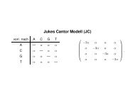
5.1. Top-down InductionIn order to create frequent patterns top-down induction isapplied. In the first step all frequent patterns of the desiredpattern size (i.e., number of used predicates) are created.Here, for all predicates new variables are created. In thesecond step, the patterns are specialized by the unificationof variables, i.e., the different predicates can be “connected”via identical variables after this step. In the third step temporalrestrictions are added to the patterns. If a maximumvalue for the number of patterns to keep (maxP atterns) isset, after each step only the best patterns are kept. The basicsteps are illustrated in Figure 1. The pattern generationalgorithm is:1. Basic pattern generation.(a) Create initial patterns (consisting of justone predicate each) and store them in thecurrentP atternsList. Set currentLevel to 1.(b) Remove all patterns from thecurrentP atternsList which do notsatisfy certain conditions (e.g., minimumfrequency). Add all patterns incurrentP atternsList to allP atternsListif currentLevel < minP atternLevel.(c) If currentLevel ≤ maxP atternLevelcreate next level patterns: ClearcurrentP atternsList, specialize all frequentpatterns by combining them with all predicatesof the frequent patterns of the previous stepand store them in the currentP atternsList.Keep the best maxP atterns patterns in theallP atternsList. Go to step 1b.2. Specialize by variable unification.(a) Set the currentP atternList toallP atternList.(b) For each pattern in currentP atternList createall possible variable unifications and store themin the cleared currentP atternList.(c) Remove all patterns from thecurrentP atternsList which do not satisfycertain conditions (e.g., minimum frequency).Add all patterns in currentP atternsList toallP atternsList.(d) If new patterns were created go to step 2b.(e) Keep the best maxP atterns patterns in theallP atternsList.3. Specialize by temporal relations.(a) Set the currentP atternList toallP atternList.(b) For each pattern create statistics about temporalrelations between predicates (i.e., count the occurrencesof the different interval relations foreach pattern pair).(c) If the creation of a temporal relation betweentwo predicates in a pattern does notviolate certain conditions (e.g., minimum frequency),the pattern is copied, specialized bythis temporal relation, and added to the clearedcurrentP atternList.(d) Add all patterns in currentP atternsList toallP atternsList. If new patterns were createdgo to step 3b.(e) Keep the best maxP atterns patterns in theallP atternsList.The parameters of the algorithm are:• minPatternLevel: The minimum size of the patterns(i.e., the minimum number of predicates appearing ineach pattern).• maxPatternLevel: The maximum size of the patterns(i.e., the maximum number of predicates appearing ineach pattern).• maxPatterns: The maximum number of patterns to bekept after each step of the algorithm.5.2. Pattern EvaluationIn order to evaluate the patterns (and to keep the k bestpatterns) an evaluation function was defined. Right now ourevaluation function takes five different values into account:relative pattern size, relative pattern frequency, coherence,temporal restrictiveness, and predicate preference. Furthercriteria can be added if necessary.The relative pattern size is the pattern size divided by themaximum pattern size:relP atSize =patSizemaxP atSizeThis measure prefers larger patterns. The assumption hereis that patterns with more predicates which are still frequentcontain more useful information than shorter ones.The relative pattern frequency is the number of matchesmultiplied by the pattern size relative to the length of thewhole sequence:relP atF rq =patSize · numMatchessequenceLength

Patterns which appear more often are assigned a highervalue.The coherence gives information how “connected” thepredicates in the pattern are by putting the number of usedvariables in relation to the maximum possible number ofvariables for a pattern:coh = 1 −numV ariablesmaxNumberV ariablesHere, the idea is that patterns which are highly connectedthrough variables provide more information because theyare interrelated by shared objects. Currently we just regardbinary predicates, thusmaxNumberV ariables = 2 · patSize.The temporal restrictiveness is the number of restrictedpredicate pairs in the pattern to the maximum number oftime restrictions:tmpRestr ==numRestrictedP redP airsmaxNumRestrictedP redP airsnumRestrictedP redP airspatSize·(patSize−1)2Again it is assumed to be advantageous if the pattern is morespecialized. A higher number of temporal restrictions leadsto a higher value.Predicate preference computes the mean of all used predicatepreferences:prP ref =patSize1 ∑preference(predicate i )patSizei=1This is needed if certain predicates should be privileged,e.g., if some predicates are assumed to be more useful thanothers.The overall evaluation function of a pattern computes aweighted sum of the five values:eval =a · relP atSize + b · relP atF rq + c · coh + d · tmpRestr + e · prP refa + b + c + d + eAll single measures and the overall pattern quality havevalues between 0 and 1.6. EvaluationThis section presents a first evaluation of our learning algorithm.First, the idea is shown by applying the algorithmto a simple example. After that experiments on some morecomplex data with varying parameters are presented. Finally,some statements about the complexity of the currentalgorithm are given.s; behind; a; bs; faster; x; ye; behind; a; bs; leftOf; a; be; leftOf; a; be; faster; x; ys; behind; b; ae; behind; b; as; behind; a; cs; approaches; x; ye; behind; a; cs; leftOf; a; ce; leftOf; a; ce; approaches; x; ys; behind; c; ae; behind; c; as; behind; a; ds; follows; x; ye; behind; a; ds; leftOf; a; de; leftOf; a; de; follows; x; ys; behind; d; ae; behind; d; as; faster; x; ze; faster; x; zFigure 2. Input for sequence exampleStep New patterns Kept patterns All patternsInitial patterns 5 5 0Pattern level 2 15 10 10Pattern level 3 28 13 23Unification 1 255 57 80Unification 2 393 51 131Unification 3 200 15 146Unification 4 32 1 147Unification 5 1 0 147Temp. Rest. 1 13 13 160Temp. Rest. 2 21 21 181Temp. Rest. 3 9 9 190Table 1. Number of patterns in the differentsteps of the algorithm6.1. Simple ExampleIn this subsection patterns for a simple artificial exampleare created. In the example there are seven different objects(a - d and x - z), five predicates (behind, faster,leftOf, approaches, and follows). The input datais shown in Figure 2. The first column gives the informationif the interval starts or ends in this row. The names of thepredicates are in the second column. The third and fourthcolumns show the IDs of the objects for which the predicateholds. The temporal order is represented by the rows fromtop to bottom.Figure 3 shows the different intervals in this example. Asit can be seen, object a has behind and leftOf relationsto the objects b, c, and d. The predicates with x, y, and zare not important; they are just “noise” in the example.The program was started with these parameters:• minP atternSize = 2,• maxP atternSize = 3, and• maxP atterns = ∞ (i.e., keep all created patterns).The weights of the evaluation function were set to: a =0.2, b = 0.4, c = 0.2, d = 0.2, and e = 0.0. The predicatepreference has not been realized so far and is thus not takeninto account here.Table 1 shows the number of patterns for the differentsteps. Note that patterns are just kept if they have more than

Figure 3. Example sequence and matched patternPatternbehind(X 9 X 29)[r 1], leftOf(X 9 X 29)[r 2], behind(X 29X 9)[r 3], r 1r 2: before, r 1r 3: before, r 2r 3:beforebehind(X 9 X 29)[r 1], leftOf(X 9 X 29)[r 2], behind(X 29X 9)[r 3], r 1r 2: before, r 1r 3: beforebehind(X 9 X 29)[r 1], leftOf(X 9 X 29)[r 2], behind(X 29X 9)[r 3], r 1r 3: before, r 2r 3: beforebehind(X 9 X 29)[r 1], leftOf(X 9 X 29)[r 2], behind(X 29X 9)[r 3], r 1r 2: before, r 2r 3: beforebehind(X 9 X 29)[r 1], leftOf(X 9 X 29)[r 2], behind(X 29X 9)[r 3], r 2r 3: beforeTable 2. Five best patternsOverallquality0.7800.7130.7130.7130.646one predicate. The five best patterns are shown in Table 2.The intended pattern in the example was a simplified overtakingscenario (first, the overtaking car is behind anothercar, then it is left of, and finally the objects in the behindpredicate are switched). As it can be seen, the intended patternwas found and evaluated best. Matched sequence partsare illustrated in Figure 3, enclosed by a dashed line.6.2. ExperimentsWe evaluated the algorithm on an artificial data set withdifferent settings. In order to create random data sets wewrote a program which generates input data for our learningprogram. Different parameters allow for creating differenttest sets. The parameters are: number of predicates,number of constants, fraction of “real patterns” in the randomdata, and the length of the sequence. As the “realpattern” the one above (behind(X, Y), leftOf(X,Y), behind(Y, X)) was used with varying constantsfor X and Y and some random predicates inside the pattern.For the experiments random sequences with 500 predicates(i.e., 1000 start and end time points) were created. Theevaluation function was the same as shown above in Section6.1. The window size was set to 15 (large enough to find theintended pattern). The number of constants (representingobjects) was five in all settings. The minimum frequency inorder to keep a pattern was 0.1. Figure 4 shows the numberof created and kept patterns for the different settings in theexperiments.The number of predicates was varied in the first experiment(5, 7, 9, and 11). One interesting fact is that with anincreasing number of predicates the number of created patternsdecreases. This seems counterintuitive at first glance.This phenomenon can be explained by the randomly createddata. The more predicates are used the less frequent patternswith (random) predicates are created. This explains the decreasingnumber of created patterns in the first experiment.In the second experiment the maximum size of the patternswas set to different values (2 - 5). This experimentshows the problem of complexity. With the increasing maximalsize of patterns the number of created patterns growsexponentially. Future modifications of the algorithm shouldaddress this problem.In the third experiment the number of patterns to keep aftereach step of the algorithm was varied (maxP atterns =5, 10, 15, 20). It shows how the number of created (andkept) patterns can be reduced by just keeping a certain numberof patterns after each step of the basic pattern generation.The number of kept patterns almost stays constant.This might be due to the fact that many of the bad performingpatterns are not created as their “parents” are prunedearly while the important patterns are kept after each step.6.3. ComplexityThe algorithm consists of three main steps. The basicpattern generation algorithm creates predicate combinationsup to an upper bound (the pattern size). If all predicatecombinations were created the number of created patternswould be equal to the number of possibilities to take k elementsout of n elements ignoring the order and allowingto draw elements repeatedly. Let n be the number of predicatesand k the maximum pattern size. Then the number ofbasic patterns to be created is:( ) n + k − 1#basicP atterns =kTable 3 shows the number of possible patterns for differentpattern sizes if five predicates exist, i.e., n = 5.The variable unification problem is similar to the problemof creating all possible clusters of arbitrary sizes for nobjects. This leads to the Bell number [4]. The number

Varying number of predicatesSize of pattern 1 2 3 4 5#possibleRestrictions 1 14 14 3 14 6 14 10#patterns#patterns#patterns0 500 1000 15000 10000 30000 500000 500 1000Generated patternsKept patterns5 6 7 8 9 10 11Generated patternsKept patterns#predicatesVarying pattern size2.0 2.5 3.0 3.5 4.0 4.5 5.0Generated patternsKept patternsPattern sizeVarying number of kept patterns5 10 15 20maxPatternsFigure 4. Evaluation resultsSize of pattern 1 2 3 4 5#possiblePatterns 5 15 35 70 126Table 3. Number of possible patterns with fivepredicatesof all possible variable combinations for n variables can becomputed by the formula (cf. [12]):n∑{ n#posV arUnific =k}=k=1n∑k=11k!k∑( ) k(−1) k−j j njj=1The Bell numbers for different n are shown in Table 4.The number of possible temporal restrictions for a patterndepends on the number of predicates used in the patternn 1 2 3 4 5 6 7 8 9 10B n 1 2 5 15 52 203 877 4140 21147 115975Table 4. Bell numbersTable 5. Number of possible temporal restrictionswith five predicatesand the number of temporal relations. It is possible to assignone of Allen’s 13 relations or no relation to each predicatepair. Of course, not all combinations are possible (e.g., ifp1 is before p2 and p2 is before p3 there p1 must be beforep3). For simplicity, we assume independency betweenthe predicate pairs for the moment. In that case for eachpredicate pair 14 variations are possible. Thus, we have tocalculate the power of 14 to the number of possible predicatepairs (n is the number of predicates in the pattern):numP redP airs#temporalRestrictions = 14= 14 n·(n−1)2Table 5 shows the number of temporal restrictions for differentpattern sizes if five predicates are used.Altogether the number of possible patterns grows veryhigh if the number of used predicates in patterns is large.First of all, many “basic patterns” are created in this case.For each of these patterns many variable unifications arepossible (depending on the number of variables in all predicatesof the pattern). In the last step for each of the unifiedpatterns many variations of temporal restrictions are possible.This shows that a modification of the algorithm hasto be done in order to make it applicable to more complexsituations.7. Conclusion and Future WorkThe approach presented here allows for learning patternsfrom sequential symbolic data. As the representation consistsof predicates which describe relations between differentobjects more complex patterns can be learned comparedto propositional event sequences. The unsupervised patternlearning algorithm performs a top-down search from themost general to more specific patterns. In the first step frequentbasic patterns are generated (similar to standard associationrule mining). In the second step variable unificationleads to an interconnection of predicates and thus to morecoherent patterns. In the third step the patterns are specializedby temporal constraints. Here, Allen’s interval logicis used to interrelate the predicates in the patterns temporarily.An evaluation function was introduced, which takes intoaccount the special properties of our pattern representation.The algorithm was implemented and tested on artificial datasets.Although the basic algorithm has been implemented alreadythere are many possibilities for future work. Even

though the incremental generation of new patterns just fromfrequent patterns excludes many unimportant patterns, thecomplexity of the algorithm is still very high. An interestingresearch direction is to find out which heuristics couldreduce complexity and still lead to good patterns. Anotherpossibility is to prevent the program from the generation ofcertain patterns by leaving out (temporal) relations whichare not possible due to some constraints. These constraintscould be identified e.g., by accessing a composition table asintroduced by Allen [3] as it was done by Höppner [5]. Insome cases it might be also possible to reduce the numberof temporal relations. If some of the 13 relations are notneeded (or do not appear in the data) they can be omitted inorder to reduce complexity.The creation of temporal restrictions is quite straightforwardso far as just one temporal relation is allowed betweentwo predicates. If the semantic is changed to “allowed temporalrelations”, more than one temporal relation could beallowed for each predicate pair. This would lead to a morepowerful representation of the temporal restrictiveness.In the current version of the algorithm just frequent patternsare generated. In future versions it would interestingto create (temporal) association rules, which can be appliedfor anticipating (possible) future events.In future work the pattern learning has to be evaluated insome application context with real data in order to evaluatehow beneficial such learned patterns can be. This can bedone in the context of intelligent agents which should uselearned patterns to improve their future behavior, e.g., byavoiding unfavorable or dangerous situations or by reusingpartial plans which have been computed in similar situationbefore to save time.8. AcknowledgementsThe content of this paper is a partial result of the ASKOFproject which is funded by the Deutsche Forschungsgemeinschaft(DFG, German Research Foundation) undergrant HE989/6-1. We would like to thank Björn Gottfried,Martin Lorenz, Ingo J. Timm, and Tom Wetjen for interestingdiscussions on the learning of patterns and complexitycalculations, and for their comments how to improve thispaper.ference on Very Large Data Bases, VLDB, pages 487–499,September 1994.[3] J. F. Allen. Maintaining knowledge about temporal intervals.Communications of the ACM, 26(11):832–843, November1983.[4] E. T. Bell. Exponential numbers. The American MathematicalMonthly, 41(7):411 – 419, August/September 1934.[5] F. Höppner. Learning temporal rules from state sequences.In Proceedings of the IJCAI’01 Workshop on Learning fromTemporal and Spatial Data, pages 25–31, Seattle, USA,2001.[6] K. Koperski and J. Han. Discovery of spatial associationrules in geographic information databases. In Proceedingsof the 4th International Symposium on Advances in SpatialDatabases, SSD, pages 47–66, Portland, Maine, 1995.[7] D. Malerba and F. A. Lisi. An ILP method for spatial associationrule mining. In Working notes of the First Workshop onMulti-Relational Data Mining, pages 18–29, Freiburg, Germany,2001.[8] H. Mannila, H. Toivonen, and A. I. Verkamo. Discoveryof frequent episodes in event sequences. Data Mining andKnowledge Discovery, 1:259–289, 1997.[9] J. Mennis and J. W. Liu. Mining association rules in spatiotemporaldata. In Proceedings of the 7th International Conferenceon GeoComputation, University of Southampton,UK, 8 - 10 September 2003.[10] A. Miene, A. D. Lattner, U. Visser, and O. Herzog.Dynamic-preserving qualitative motion description for intelligentvehicles. In Proceedings of the IEEE IntelligentVehicles Symposium (IV ’04), pages 642–646, June 14-172004.[11] A. Miene, U. Visser, and O. Herzog. Recognition and predictionof motion situations based on a qualitative motiondescription. In D. Polani, B. Browning, A. Bonarini, andK. Yoshida, editors, RoboCup 2003 – Proceedings of theInternational Symposium, July 10.-11., 2003, Padua, Italy,2003.[12] J. Pitman. Some probabilistic aspects of set partitions. TheAmerican Mathematical Monthly, 104(3):201–209, March1997.[13] P.-N. Tan, V. Kumar, and J. Srivastava. Selecting the right interestingnessmeasure for association patterns. In Proceedingsof the Eight International Conference on KnowledgeDiscovery and Data Mining (KDD’02), pages 32–41, 2002.[14] M. J. Zaki, S. Parthasarathy, M. Ogihara, and W. Li. Newalgorithms for fast discovery of association rules. In Proceedingsof the 3rd International Conference on KnowledgeDiscovery and Data Mining, pages 283–296, 1997.References[1] R. Agrawal, T. Imielinski, and A. N. Swami. Mining associationrules between sets of items in large databases. InProceedings of the 1993 ACM SIGMOD International Conferenceon Management of Data, pages 207–216, Washington,D.C., May 1993.[2] R. Agrawal and R. Srikant. Fast algorithms for mining associationrules. In Proceedings of the 20th International Con-