Multirate Anypath Routing in Wireless Mesh Networks - Leonard ...

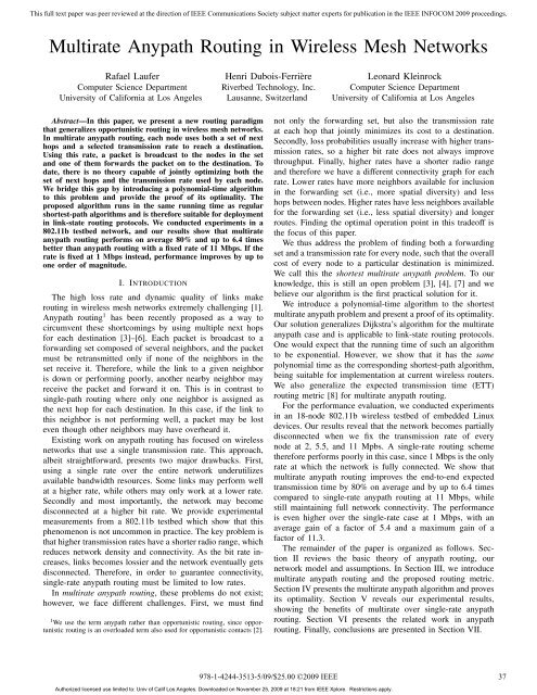
This full text paper was peer reviewed at the direction of IEEE Communications Society subject matter experts for publication in the IEEE INFOCOM 2009 proceedings.sFigure 3. A multirate anypath connecting nodes s and d is shown in boldarrows. Every packet sent from s traverses a path to reach d, such as thepath shown with dashed lines. Different dash lengths represent the differentbit rates used by each node, with a shorter dash for higher rates.In real wireless networks, we usually have different deliveryprobabilities and distances for each transmission rate, whichjustifies this model extension.The EATX metric described in Section II-C was originallydesigned considering that nodes transmit at a single bit rate.To account for multiple bit rates, we introduce the expectedanypath transmission time (EATT) metric. For EATT, thehyperlink distance d (r)iJfor each rate r ∈ R is defined asd (r)iJ = 1 × sp (r) r , (5)iJwhere p (r)iJis the hyperlink delivery probability defined in (1),s is the maximum packet size, and r is the bit rate. Thedistance d (r)iJis basically the time it takes to transmit a packetof size s at a bit rate r over a lossy hyperlink with deliveryprobability p (r)iJ. The EATT metric is a direct generalizationof the expected transmission time (ETT) metric [8] commonlyused in single-path wireless routing. Note that for each bit rater ∈ R, we have a different delivery probability p (r)iJ , whichusually decreases for higher rates. This behavior imposes atradeoff; a higher bit rate decreases the time of a single packettransmission (i.e., s/r decreases), but it usually increasesthe number of transmissions required for a packet to besuccessfully received (i.e., 1/p (r)iJ increases).The remaining-anypath cost D (r)Jnow also depends on thetransmission rate, since the delivery probabilities change foreach rate. Since both the hyperlink distance and the remaininganypath cost depend on the bit rate, node i has a differentanypath cost D (r)i = d (r)iJ+ D(r) Jfor each forwarding set Jand for each transmission rate r ∈ R.We address the problem of finding both the forwardingset and the transmission rate that minimize the overall costto reach a particular destination. We call this the shortestmultirate anypath problem, which generalizes the shortestanypathproblem [6] for the multirate scenario. Interestingly,the shortest multirate anypath will always have equal or lowercost than the shortest single path. Among all possible multirateanypaths between two nodes, we also have the single path withthe shortest ETT. As a result, the cost of the shortest multirateanypath can never be higher than the cost of the shortest path.Likewise, due to the same argument, the shortest multirateanypath will also have equal or lower cost than any shortestanypath using a single rate.dIV. FINDING THE SHORTEST MULTIRATE ANYPATHIn this section we introduce the proposed shortest-anypathalgorithms. In Section IV-A, we present the Shortest AnypathFirst (SAF) algorithm used in a single-rate network with theEATX metric. Our SAF algorithm, while derived independently,is similar to the single-rate algorithm proposed byChachulski [3]. Our main contribution is to provide a proofof its optimality. We also use the single-rate case as the basisfor the multirate generalization introduced in Section IV-B.Surprisingly, the Shortest Multirate Anypath First (SMAF)algorithm has the same running time as a shortest single-pathalgorithm for multirate, being suitable for deployment in linkstaterouting protocols. We only show the proof of optimalityof the SMAF algorithm, since by definition this also impliesthe optimality of the SAF algorithm.A. The Single-Rate CaseWe now present the Shortest Anypath First algorithm usedin the simpler single-rate scenario. Given a graph G = (V,E),thealgorithmcalculatestheshortestanypathsfromallnodestoa destination d. For every node i ∈ V we keep an estimate D i ,which is an upper-bound on the distance of the shortestanypath from i to d. In addition, we also keep a forwardingset F i for every node, which stores the set of nodes used asthe next hops to reach d. Finally, we keep two data structures,namely S and Q. The S set stores the set of nodes for whichwe already have a shortest anypath defined. We store eachnode i ∈ V − S for which we still do not have a shortestanypath in a priority queue Q keyed by their D i values.SHORTEST-ANYPATH-FIRST(G,d)1 for each node i in V2 do D i ← ∞3 F i ← ∅4 D d ← 05 S ← ∅6 Q ← V7 while Q ≠ ∅8 do j ← EXTRACT-MIN(Q)9 S ← S ∪ {j}10 for each incoming edge (i,j) in E11 do J ← F i ∪ {j}12 if D i > D j13 then D i ← d iJ + D J14 F i ← JAs in the shortest-path algorithm, the Shortest Anypath Firstalgorithm is composed of |V | rounds, dictated by the numberof elements initially in Q. At each round, the EXTRACT-MINprocedure extracts the node with the minimum distance tothe destination from Q. Let this node be j. At this point,j is settled and inserted into S, since the shortest anypathfrom j to the destination is now known. For each incomingedge (i,j) ∈ E, we check if the distance D i is larger than thedistance D j . If that is the case, then node j is added to theforwarding set F i and the distance D i is updated.Figure 4 shows the execution of Shortest Anypath Firstalgorithm using the EATX metric. We see in Figure 4(a) thegraph right after the initialization. Figures 4(b)–4(h) show40Authorized licensed use limited to: Univ of Calif Los Angeles. Downloaded on November 25, 2009 at 18:21 from IEEE Xplore. Restrictions apply.

8This full text paper was peer reviewed at the direction of IEEE Communications Society subject matter experts for publication in the IEEE INFOCOM 2009 proceedings.13881456588143827d0813881564452143727d08138715 26 142.54 35727d08135.216.55 26 142.54 35727d0(a)(b)(c)(d)6.2135.216.55 26 142.54 35727d06.2135.216.55 26 142.54 35727d06.2135.216.55 26 142.54 35727d06.2135.216.55 26 142.54 35727d0(e)(f)(g)(h)Figure 4. Execution of the Shortest Anypath First (SAF) algorithm from every node to d. The weight of each link is the expected number of transmissions(ETX), which is the inverse of the link delivery probability. (a) The situation just after the initialization. (b)–(h) The situation after each successive iterationof the algorithm. Part (h) shows the situation after the last node is settled.each iteration of the algorithm. At each step, the value insidea node i presents the distance D i from that node to thedestination d and the arrows in boldface present the shortestanypath to d.Nodes withtwocirclesarethesettlednodes in S.The graph in Figure 4(h) shows the result of SAF algorithmright after settling the last node.The running time of the Shortest Anypath First algorithmdepends on how Q is implemented. Assuming that we havea Fibonacci heap, the cost of each of the |V | EXTRACT-MINoperations inline 8takes O(log V ),withatotalof O(V log V )aggregated time. The running time to calculate both d iJ andD J in line 13 depends on the size of J; however, if we storeadditional state, it can be reduced to a constant time [10]. Thefor loop of lines 10–13 takes O(E) aggregated time and as aresult the total complexity of the algorithm is O(V log V +E),which is the same complexity of Dijkstra’s algorithm.B. The Multirate CaseWe now generalize the SAF algorithm to support multipletransmission rates, introducing the Shortest Multirate AnypathFirst (SMAF) algorithm. For each node i ∈ V, we nowkeep a different distance estimate D (r)i for every rate r ∈ R.The estimate D (r)i is an upper-bound on the distance of theshortest anypath from i to d using transmission rate r. Inaddition, we also keep its corresponding forwarding set F (r)i ,which stores the set of next hops used for i to reach dusing r. We use D i and F i without the indicated rates tostore the minimum distance estimate among all rates and itscorresponding forwarding set, respectively. We also keep atransmission rate T i for every node, which stores the rate usedto reach d.The key idea of the SMAF algorithm is that each nodei ∈ V has an independent distance estimate D (r)i for each rater ∈ R and we keep the minimum of these estimates as thenode distance D i . At each round of the while loop, the nodewith the minimum distance from Q is settled. Let this nodebe j. For each incoming edge (i,j) ∈ E, we check for everyrate r ∈ R ifthedistance D (r) islargerthanthedistance D j ofithe node just settled. If that is the case, then node j is added tothe forwarding set F (r)i of that specific rate and distance D (r)iis updated accordingly. If the new distance D (r) is shorter thanthe node distance D i , we update the node distance D i as welliSHORTEST-MULTIRATE-ANYPATH-FIRST(G,d)1 for each node i in V2 do D i ← ∞3 F i ← ∅4 T i ← NIL5 for each rate r in R6 do D (r)i ← ∞7 F (r)i ← ∅8 D d ← 09 S ← ∅10 Q ← V11 while Q ≠ ∅12 do j ← EXTRACT-MIN(Q)13 S ← S ∪ {j}14 for each incoming edge (i,j) in E15 do for each rate r in R16 do J ← F (r)i17 if D (r)i∪ {j}> D j18 then D (r)i19 F (r)i← d (r)iJ← J20 if D i > D (r)i+ D(r) J21 then D i ← D (r)i22 F i ← F (r)i23 T i ← ras the forwarding set F i and transmission rate T i to reflect thenew minimum.The running time of the Shortest Multirate Anypath Firstalgorithm also depends on the implementation of Q. Theinitialization in lines 1–10 takes O(V R) time. Assuming thatwe have a Fibonacci heap, the EXTRACT-MIN operations inline 12 take a total of O(V log V ) aggregated time. We assumethat the distance calculation of d (r)iJand D (r)Jin line 18 isoptimized to take a constant time [10]. As a result, the forloop in lines 15–23 takes O(ER) aggregated time. The totalrunning time is therefore O(V log V + (E + V )R), which isO(V log V +ER) if all nodes are able to reach the destination.This is the same running time of the shortest single-pathalgorithm for multiple rates. Compared to the SAF algorithm,the SMAF algorithm allows nodes to take advantage of theirmultiple transmission rates at the cost of just a small increasein the running time.41Authorized licensed use limited to: Univ of Calif Los Angeles. Downloaded on November 25, 2009 at 18:21 from IEEE Xplore. Restrictions apply.

This full text paper was peer reviewed at the direction of IEEE Communications Society subject matter experts for publication in the IEEE INFOCOM 2009 proceedings.In order to prove the optimality of the algorithm, we firstintroduce five lemmas that show a few properties of multirateanypath routing. We use δ (r)i as the distance of the shortestmultirate anypath from a node i to the destination d, when itransmits at a fixed rate r ∈ R. Likewise, φ (r)i represents thecorresponding forwarding set used in this multirate anypath.We use δ i without the indicated rate to represent the distanceof the shortest multirate anypath from i to d via the optimalforwardingset φ i andoptimaltransmissionrate ρ ∈ R.Thatis,δ i = min r∈R δ (r)i , ρ = argmin r∈R δ (r)i , and φ i = φ (ρ)i . Weuse D i as the distance of a particular multirate anypath from ito d, but not necessarily the shortest one. The proof for eachof these lemmas is available in [10].Lemma 1: For a fixed transmission rate, let D i be thedistance of a node i via forwarding set J and let D i ′ be thedistance via forwarding set J ′ = J ∪{n}, where D n ≥ D j forevery node j ∈ J. We have D i ′ ≤ D i if and only if D i ≥ D n .We use Lemma 1 for the comparisons in line 12 of theSAF algorithm and in line 17 of the SMAF algorithm. By thislemma, if the distance D i via J is larger than the distance D nof a neighbor node n, with D n ≥ D j for all j ∈ J, then thedistance D i ′ via J ′ = J ∪ {n} is always smaller than D i . Thatis, it is always beneficial to include node n in the forwardingset in order to obtain a shorter distance to the destination.Lemma 2: The shortest distance δ i of a node i is alwayslarger than or equal to the shortest distance δ j of any node jin the optimal forwarding set φ i . That is, we have δ i ≥ δ j forall j ∈ φ i .Lemma 2 guarantees that if a node i uses another node jin its optimal forwarding set φ i , then distance δ i can neverbe smaller than δ j . This is equivalent to the restriction thatall weights in the graph must be nonnegative in Dijkstra’salgorithm.Lemma 3: For any transmission rate, if a node i uses anode n in its optimal forwarding set φ i and δ i = δ n , we cansafely remove n from φ i without changing δ i . The link (i,n)is said to be “redundant.”By Lemma 3, if the distances δ i = δ n of two nodes i and nare the same, then the distance δ i via forwarding set φ i isthe same as the distance via forwarding set φ i − {n}. Thatis, the distance of node i does not change if it uses n in itsforwarding set or not.Lemma 4: If the shortest distances from the neighbors ofa node i to a given destination are δ 1 ≤ δ 2 ≤ ... ≤ δ n ,then φ (r)i is always of the form φ (r)i = {1,2,...,k}, for somek ∈ {1,2,...,n}.According to Lemma 4, the best forwarding set φ (r)i fortransmission rate r ∈ R is a subset of neighbors with theshortest distances to the destination. That is, given a setof neighbors with distances δ 1 ≤ δ 2 ≤ ... ≤ δ n , thebest forwarding set φ (r)i when using rate r ∈ R is alwaysone of {1}, {1,2}, {1,2,3},...,{1,2,...,n}. As a result,forwarding sets with gaps between the neighbors, such as{2,3} or {1,4}, can never yield the shortest distance to thedestination. This property is the key factor that allows usto reduce the complexity of the proposed algorithms fromexponential to polynomial time. For n neighbors, we do nothave to test every one of the 2 n − 1 possible forwarding sets.Instead, we only need to check at most n forwarding sets.Lemma 5: For a given transmission rate r ∈ R, assumethat φ (r)i = {1,2,...,n} with distances δ 1 ≤ δ 2 ≤ ... ≤ δ n .If D j i is the distance from node i using transmission rate r viaforwarding set {1,2,...,j}, for 1 ≤ j ≤ n, then we alwayshave Di 1 ≥ D2 i ≥ ... ≥ Dn i = δ (r)i .Lemma 5 explains another important property necessary forthe SMAF algorithm to converge. Assuming now that the bestforwarding set φ (r)i for transmission rate r ∈ R is defined as= {1,2,...,n} with distances δ 1 ≤ δ 2 ≤ ... ≤ δ n , thedistance D i monotonically decreases as we use each of theforwarding sets {1}, {1,2}, {1,2,3},...,{1,2,...,j}.We now present the proof of optimality of the algorithm.Theorem 1: Optimality of the algorithm.Let G = (V,E) be a weighted, directed, graph and let d bethe destination. After running the Shortest Multirate AnypathFirst algorithm on G, we have D i = δ i for all nodes i ∈ V.Proof: This proof is similar to the proof of Dijkstra’salgorithm [13]. We show that for each node s ∈ V, we haveD s = δ s at the time s is added to S.Forthepurposeofcontradiction,let sbethefirstnodeaddedto S for which D s ≠ δ s . We must have s ≠ d because d isthe first node added to S and D d = δ d = 0 at that time. Justbefore adding s to S, we also have that S is not empty, sinces ≠ dand S mustcontainatleast d.Weassumethattheremustbe a multirate anypath from s to d, otherwise D s = δ s = ∞,which contradicts our initial assumption that D s ≠ δ s . If thereis at least one multirate anypath, there is a shortest multirateanypath α from s to d. Let us consider a cut (V − S,S)of α, such that we have s ∈ V − S and d ∈ S, as shown inFigure 5. Let the set J be composed of nodes in V − S thathave an outgoing link to a node in S. Likewise, let the set Kbe composed of nodes in S that have an incoming link froma node in V − S.φ (r)isV − SJiFigure 5. The shortest multirate anypath α from s to d. Set S must benonempty before node s is inserted into it, since it must contain at least d.We consider a cut (V −S, S) of α, such that we have s ∈ V −S and d ∈ S.Nodes s and d are distinct but we may have no hyperlinks between s and J,such that J = {s}, and also between K and d, such that K = {d}.Without loss of generality, assume that node i ∈ J has theshortest distance to d among all nodes in V − S. That is,δ i ≤ δ j for all j ∈ V − S. We claim that every edge leavingnode i must necessarily cross the cut (V − S,S). Thus, forevery edge (i,j) leaving node i, we must have j ∈ S. Toprove this claim, let us assume that node i has an edge (i,j)to another node j ∈ V − S. By Lemma 2, we know that inthis case we must have δ i ≥ δ j . However, since we assumedthat node i has the shortest distance in V − S, then δ i ≤ δ jKSd42Authorized licensed use limited to: Univ of Calif Los Angeles. Downloaded on November 25, 2009 at 18:21 from IEEE Xplore. Restrictions apply.