Minitab Lab Answers

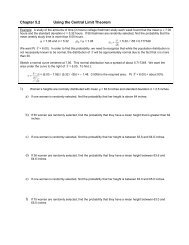
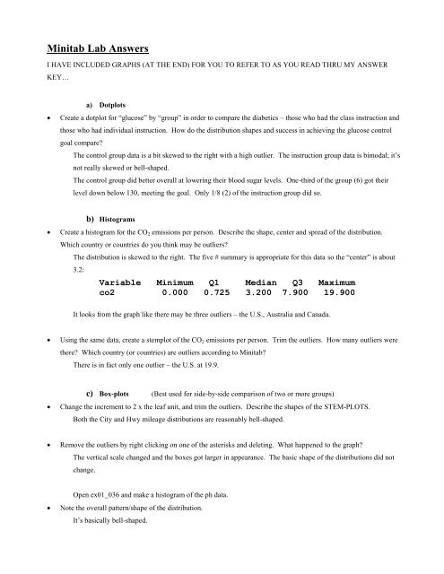
Minitab Lab AnswersI HAVE INCLUDED GRAPHS (AT THE END) FOR YOU TO REFER TO AS YOU READ THRU MY ANSWERKEY…a) DotplotsCreate a dotplot for “glucose” by “group” in order to compare the diabetics – those who had the class instruction andthose who had individual instruction. How do the distribution shapes and success in achieving the glucose controlgoal compare?The control group data is a bit skewed to the right with a high outlier. The instruction group data is bimodal; it’snot really skewed or bell-shaped.The control group did better overall at lowering their blood sugar levels. One-third of the group (6) got theirlevel down below 130, meeting the goal. Only 1/8 (2) of the instruction group did so.b) HistogramsCreate a histogram for the CO 2 emissions per person. Describe the shape, center and spread of the distribution.Which country or countries do you think may be outliers?The distribution is skewed to the right. The five # summary is appropriate for this data so the “center” is about3.2:Variable Minimum Q1 Median Q3 Maximumco2 0.000 0.725 3.200 7.900 19.900It looks from the graph like there may be three outliers – the U.S., Australia and Canada.Using the same data, create a stemplot of the CO 2 emissions per person. Trim the outliers. How many outliers werethere? Which country (or countries) are outliers according to Minitab?There is in fact only one outlier – the U.S. at 19.9.c) Box-plots (Best used for side-by-side comparison of two or more groups)Change the increment to 2 x the leaf unit, and trim the outliers. Describe the shapes of the STEM-PLOTS.Both the City and Hwy mileage distributions are reasonably bell-shaped.Remove the outliers by right clicking on one of the asterisks and deleting. What happened to the graph?The vertical scale changed and the boxes got larger in appearance. The basic shape of the distributions did notchange.Open ex01_036 and make a histogram of the ph data.Note the overall pattern/shape of the distribution.It’s basically bell-shaped.

Make a simple box-plot of the ph data and describe how the shape of the distribution is reflected in the box-plot.The whiskers are about the same length and the median line is about in the middle of the box. This is consistentwith the reasonably symmetric bell shape of the distribution.d) Time PlotsEdit the Y scale (right click on the vertical axis) and change the minimum to 54. What happened to the appearanceof the graph?The scale changed (of course), making the year to year changes less “drastic” looking.Make a histogram of the Pasadena temperatures. Describe the distribution (shape, center, spread, outliers).The data is bell-shaped with no outliers. The mean is 64.25° and the standard deviation is about 1.2°.Summarizing Quantitative Date with Basic StatisticsFind the mean and median for City and Hwy mileages (use Stat > Basic Statistics > Display Descriptive Statistics).How do they compare?City: mean is 18.18, median is 17.5 Hwy: mean is 25.18, median is 24.5In each case, the mean is a little higher than the median. This is due to the high outlier. Without the outlier, we haveCity: mean is 16.9, median is 17 Hwy: mean is 23.9, median is 24Now in each case the mean is very close to the median.Find the mean of the Pasadena average annual temperatures. Find the median as well. How do these two measuresof center compare? Why would you expect this after seeing the shape of the distribution?The mean is 64.25° and the median is 64.24° - they are very close. You expect this with a distribution that issymmetric and bell-shaped.NOTE: Because the distribution is symmetric we expect them to be close. BUT just because they are close does NOTmean that we can conclude the distribution is bell-shaped!!! There is a big difference!

Using the sole data (Ex10_034), make a time plot (use a Scatterplot (With Connect Line)). Use Time on the X axis.Describe the overall pattern seen in the time plot.The trend us upward until the number of recruits peaked in the mid-1980s; then the trend is downward so that thelevels have fallen back to levels similar to those in the 1970s.NOTE: IT IS not CORRECT TO USE TERMS LIKE “BELL-SHAPED”, UNIMODAL OR SKEWEDto describe a time plot! Also, there is NO seasonal variation in this plot. Now find the mean and median of the recruitment of rock sole in the Bering Sea data (use Stat > Basic Statistics >Display Descriptive Statistics).The mean is 1120 and the median is 702.Make a stem-plot of the data. Describe the shape of the distribution. Trim the outlier(s) in your stem-plot.The distribution is skewed to the right with one strong outlier.Remove the outlier(s) from your data as well and calculate the mean and median again. What effect does removingthe outlier(s) have on the values of the mean and the median?The mean went down to only 987; the median went down just a bit to 676. Both decreased, but the meanchanged more than the median did. (This illustrates the fact that the mean is a non-resistant measure whilethe median is a resistant measure.)Some of you said that the mean and median did not change – this is impossible!Some of you said that the mean went down but the median did not change. It DID change… but it did notgo down as much as the mean.Following are the graphs. I have included some normal probability plots as well – note how theyappear for skewed data, and for normal data.

PercentgroupDotplot of glucoseci80120160200 240glucose280320360Probability Plot of classNormal - 95% CI99959080706050403020Mean 163.3StDev 70.66N 18AD 0.911P-Value 0.01610510100200class300400

FrequencyPercentProbability Plot of individualNormal - 95% CI99959080706050403020Mean 190.1StDev 41.90N 16AD 0.426P-Value 0.277105150100150200individual25030035016Histogram of co21412108642004812co21620

Stem-and-leaf of co2 N = 48Leaf Unit = 1.020 0 00000000000000011111(9) 0 22223333319 0 44516 0 667712 0 8889996 1 0013 13 13 1 67HI 19Stem-and-leaf of City N = 34Leaf Unit = 1.02 0 994 1 018 1 222311 1 45517 1 66677717 1 88889911 2 0000015 2 233 2 52 2 6HI 60Stem-and-leaf of Hwy N = 34Leaf Unit = 1.01 1 32 1 55 1 6677 1 998 2 016 2 22333333(3) 2 45515 2 666711 2 88889994 3 13 3 22HI 66

DataData70Boxplot of City, Hwy605040302010TypeMCityTMHwyTBoxplot of City, Hwy353025201510TypeMCityTMHwyT

phFrequency18Histogram of ph16141210864204.44.85.25.6ph6.06.46.87.0Boxplot of ph6.56.05.55.04.54.0

Y-DataPercentProbability Plot of phNormal - 95% CI99.9999590Mean 5.426StDev 0.5379N 105AD 0.300P-Value 0.5778070605040302010510.1345ph67Scatterplot of pasadena, reading vs year6766Variablepasadenareading656463626160591950196019701980year19902000

FrequencyY-Data67.565.0Scatterplot of pasadena, reading vs yearVariablepasadenareading62.560.057.555.01950196019701980year19902000Histogram of pasadena9876543210626364pasadena6566

sole5000Scatterplot of sole vs year400030002000100001970197519801985year199019952000Descriptive Statistics: soleVariable N Mean StDev Minimum Q1 Median Q3 Maximumsole 28 1120 1006 173 430 702 1634 4700Stem-and-leaf of sole N = 28Leaf Unit = 1008 0 12233344(8) 0 5555667912 1 012447 1 7774 2 242 2 8HI 47Descriptive Statistics: soleVariable N Mean StDev Minimum Q1 Median Q3 Maximumsole 27 987 735 173 425 676 1431 2809