Physics Reports ChernâSimons modified general relativity

More documents

Recommendations

Info

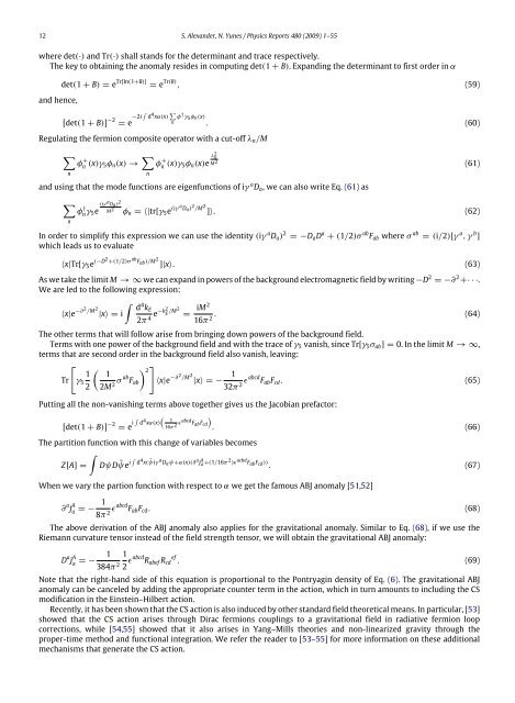
12 S. Alexander, N. Yunes / Physics Reports 480 (2009) 1–55where det(·) and Tr(·) shall stands for the determinant and trace respectively.The key to obtaining the anomaly resides in computing det(1 + B). Expanding the determinant to first order in αand hence,det(1 + B) = e Tr[ln(1+B)] = e Tr(B) , (59)∫[det(1 + B)] −2 = e −2i d 4 xα(x) ∑ φ Ď γ 5 φ n (x)n . (60)Regulating the fermion composite operator with a cut-off λ n /M∑φ + (x)γ n 5φ n (x) → ∑nnφ + (x)γ λ 2 nn 5φ n (x)e M 2 (61)and using that the mode functions are eigenfunctions of iγ a D a , we can also write Eq. (61) as∑nφ Ď γ (iγ a Da) 2Mn 5e2 φ n = 〈|tr[γ 5 e (iγ a D a ) 2 /M 2 ]〉. (62)In order to simplify this expression we can use the identity (iγ a D a ) 2 = −D a D a + (1/2)σ ab F ab where σ ab = (i/2)[γ a , γ b ]which leads us to evaluate〈x|Tr[γ 5 e (−D2 +(1/2)σ ab F ab )/M 2 ]|x〉. (63)As we take the limit M → ∞ we can expand in powers of the background electromagnetic field by writing −D 2 = −∂ 2 +· · ·.We are led to the following expression:∫〈x|e −∂2 /M 2 d 4 k E|x〉 = i2π 4 e−k2 E /M2 = iM216π . (64)2The other terms that will follow arise from bringing down powers of the background field.Terms with one power of the background field and with the trace of γ 5 vanish, since Tr[γ 5 σ ab ] = 0. In the limit M → ∞,terms that are second order in the background field also vanish, leaving:Tr[γ 512( 12M 2 σ ab F ab) 2]〈x|e −∂2 /M 2 |x〉 = − 132π 2 ɛabcd F ab F cd . (65)Putting all the non-vanishing terms above together gives us the Jacobian prefactor:∫ ([det(1 + B)] −2 = e i d 4 xα(x) 116π 2 ɛabcd F ab F cd). (66)The partition function with this change of variables becomes∫Z[A] = DψD ¯ψe ∫ i d 4 x( ¯ψiγ a D a ψ+α(x)(∂ a j A a +(1/16π 2 )ɛ acbd F ab F cd )) . (67)When we vary the partion function with respect to α we get the famous ABJ anomaly [51,52]∂ a j A a = − 18π 2 ɛabcd F ab F cd . (68)The above derivation of the ABJ anomaly also applies for the gravitational anomaly. Similar to Eq. (68), if we use theRiemann curvature tensor instead of the field strength tensor, we will obtain the gravitational ABJ anomaly:D a j A a = − 1384π 2 12 ɛabcd R abef R cd ef . (69)Note that the right-hand side of this equation is proportional to the Pontryagin density of Eq. (6). The gravitational ABJanomaly can be canceled by adding the appropriate counter term in the action, which in turn amounts to including the CSmodification in the Einstein–Hilbert action.Recently, it has been shown that the CS action is also induced by other standard field theoretical means. In particular, [53]showed that the CS action arises through Dirac fermions couplings to a gravitational field in radiative fermion loopcorrections, while [54,55] showed that it also arises in Yang–Mills theories and non-linearized gravity through theproper-time method and functional integration. We refer the reader to [53–55] for more information on these additionalmechanisms that generate the CS action.
S. Alexander, N. Yunes / Physics Reports 480 (2009) 1–55 133.2. String theoryIn the previous section, we derived the chiral anomaly in a 3 + 1 gauge field theory coupled to fermions. We saw that,while gauge and global anomalies can exist, gauge anomalies need to be cancelled to have a consistent quantum theory. Inwhat follows, we will show how the CS modification to general relativity arises from the Green–Schwarz anomaly cancelingmechanism in heterotic String Theory. The key idea is that a quantum effect due to a gauge field that couples to the stringinduces a CS term in the effective low energy four dimensional general relativity.Recall that the action of a free, one-dimensional particle can be described as the integral of the worldline swept out overa ‘‘target spacetime’’ X a (τ), parametrized by τ . The infinitesimal path length swept out isdl = (−ds 2 ) 1/2 = (−dX a dX b η ab ) 1/2 (70)where η ab is a 9 + 1D Minkowski target space-time and the action is then∫ ∫S = −mdl = −mdτ(−Ẋ a Ẋ a ) 1/2 . (71)We can easily extend the discussion of a point particle to a string by parametreizing the worldsheet with a target functionin terms of two coordinates (σ , τ). Consider then the string, world-sheet field X a (σ , τ) embedded in a D-dimensional spacetime,G ab that sweeps out a 1+1 world-sheet denoted by coordinates (σ , τ) and world-sheet line element ds 2 = h AB dX A dX B .The indices A, B here run over world-sheet coordinates. Analogous to the point particle, the free string action is describedbyS st = T ∫ds = T ∫dσ dτ √ −hh AB ∂ a X A (σ , τ)∂ b X B (σ , τ)G ab , (72)2 2where T is the string tension.This string is also charged under a U(1) symmetry and couples to the Neveu–Schwarz two-form potential, B µν , via∫S B = d 2 σ ∂ a X(σ , τ)∂ b X(σ , τ)B ab . (73)It is this fundamental string field B ab that underlies the emergence of CS modified gravity when String Theory is compactifiedto 4D. In a seminal work, Alvarez-Gaume and Witten [56] showed that GR in even dimensions will suffer from a gravitationalanomaly in a manner analogous to how anomalies are realized in the last section. The low-energy limit of superstringtheories are 10 dimensional supergravity (SUGRA) theories. As discussed in the previous section, a triangle loop diagrambetween gravitons and fermions will generate a gravitational anomaly; similarly hexagon loop diagrams generate anomaliesin 10 dimensions. Remarkably, Green and Schwarz [57,58] demonstrated that the gravitational anomaly is cancelled from aquantum effect of the string worldsheet B field, since the string worldsheet couples to a two form, B ab . The stringy quantumcorrection shifts the gradient of the B ab field by a CS 3-form. This all results in modifying the three-form gauge field strengthtensor H abc in 10D supergravity.H abc = (dB) abc → (dB) abc + 1 4(Ωabc (A) − α ′ Ω abc (ω) ) . (74)This naive shifting of H abc conspires to cancel the String Theory anomaly. We refer the interested reader to Vol II ofPolchinski’s book [59] for a more detailed discussion of the Green–Schwarz anomaly canceling mechanism.We begin our analysis from the compactification of the heterotic string to its 4D, N = 1 supergravity limit. Forconcreteness we consider the compactification to be on six dimensional internal space (i.e. a Calabi–Yau manifold). Similarto the Kaluza–Klein idea, when we dimensionally reduce a 10 dimensional system to four dimensions, many fields (moduli)which characterize the geometry emerge. These fields cause a moduli problem since their high energy density will overclosethe universe, hence, they need to be stabilized. The discussion of moduli stabilization is beyond the scope of this review andwe point the reader interested in this field of research to the work of Gukov et al. [60]. In what follows, we will assume thatall moduli except the axion are stabilized and will not explicitly deal with them in our analysis.Our starting point is the 10D Heterotic string action in Einstein frame [61] and we ignore the coupling to fermionic fieldssince they are not relevant for our discussion. In this theory the relevant bosonic field content is the 10D metric, g ab , a dilatonφ and a set of two and three form field strength tensors H 3 := H abc and F 2 := F ab respectively.∫S = d 10 x √ [g 10 R − 1 2 ∂ aφ∂ a φ − 112 e−φ H abc H abc − 1 ]4 e −φ2 Tr(F ab F ab ) , (75)whereH 3 = dB 2 − 1 4(Ω3 (A) − α ′ Ω 3 (ω) ) , (76)
Page 1 and 2: Physics Reports 480 (2009) 1-55Cont
Page 3 and 4: S. Alexander, N. Yunes / Physics Re
Page 11: S. Alexander, N. Yunes / Physics Re
Page 55: S. Alexander, N. Yunes / Physics Re

Physics Reports ChernâSimons modified general relativity

You also want an ePaper? Increase the reach of your titles

Delete template?

Save as template?

Physics Reports ChernâSimons modified general relativity