Physics Reports Chern–Simons modified general relativity

Physics Reports 480 (2009) 1–55Contents lists available at ScienceDirectPhysics Reportsjournal homepage: www.elsevier.com/locate/physrepChern–Simons modified general relativityStephon Alexander a,c , Nicolás Yunes b,c,∗a Department of Physics and Astronomy, Haverford College, Haverford, PA 19041, USAb Department of Physics, Princeton University, Princeton, NJ 08544, USAc Institute for Gravitation and the Cosmos, Department of Physics, The Pennsylvania State University, University Park, PA 16802, USAa r t i c l ei n f oa b s t r a c tArticle history:Accepted 25 July 2009Available online 29 July 2009editor: M.P. KamionkowskiPACS:11.30.Er04.60.Cf04.60.Bc04.50.Kd04.30.Tv04.80.CcChern–Simons modified gravity is an effective extension of general relativity that capturesleading-order, gravitational parity violation. Such an effective theory is motivated byanomaly cancelation in particle physics and string theory. In this review, we begin byproviding a pedagogical derivation of the three distinct ways such an extension arises: (1) inparticle physics, (2) from string theory and (3) geometrically. We then review many exactand approximate vacuum solutions of the modified theory, and discuss possible mattercouplings. Following this, we review the myriad astrophysical, solar system, gravitationalwave and cosmological probes that bound Chern–Simons modified gravity, includingdiscussions of cosmic baryon asymmetry and inflation. The review closes with a discussionof possible future directions in which to test and study gravitational parity violation.© 2009 Published by Elsevier B.V.Keywords:ChernSimonsString theoryLoop Quantum GravityParity violationContents1. Introduction............................................................................................................................................................................................. 22. The ABC of Chern–Simons and its tools................................................................................................................................................. 32.1. Formulation................................................................................................................................................................................. 32.2. Non-dynamical CS gravity and the Pontryagin constraint....................................................................................................... 62.3. Dynamical CS gravity.................................................................................................................................................................. 82.4. Parity violation in CS modified gravity...................................................................................................................................... 82.5. Boundary issues .......................................................................................................................................................................... 93. The many faces of Chern–Simons gravity ............................................................................................................................................. 103.1. Particle physics ........................................................................................................................................................................... 103.2. String theory ............................................................................................................................................................................... 133.3. Loop Quantum Gravity ............................................................................................................................................................... 144. Exact vacuum solutions .......................................................................................................................................................................... 154.1. Classification of general solutions ............................................................................................................................................. 154.2. Spherically symmetric spacetimes ............................................................................................................................................ 164.3. Why is the Kerr metric not a solution in CS modified gravity? ............................................................................................... 17∗ Corresponding address: Department of Physics, Princeton University, Institute for Gravitation and the Cosmos, Princeton, NJ 08544, USA.E-mail addresses: sha3@psu.edu (S. Alexander), nyunes@princeton.edu (N. Yunes).0370-1573/$ – see front matter © 2009 Published by Elsevier B.V.doi:10.1016/j.physrep.2009.07.002

2 S. Alexander, N. Yunes / Physics Reports 480 (2009) 1–554.4. Static and axisymmetric spacetimes ......................................................................................................................................... 174.5. Stationary and axisymmetric spacetimes ................................................................................................................................. 184.6. pp-waves and boosted black holes ............................................................................................................................................ 194.7. Non-axisymmetric solutions and matter .................................................................................................................................. 195. Approximate vacuum solutions ............................................................................................................................................................. 205.1. Formal post-Newtonian solution............................................................................................................................................... 205.2. Parameterized post-Newtonian expansion............................................................................................................................... 215.3. Rotating extended bodies and the gravitomagnetic analogy................................................................................................... 235.4. Perturbations of the Schwarzschild spacetime......................................................................................................................... 255.5. Slowly rotating Kerr-like black holes ........................................................................................................................................ 275.6. Gravitational wave propagation ................................................................................................................................................ 295.7. Gravitational wave generation .................................................................................................................................................. 326. Non-vaccum solutions and Fermionic interactions .............................................................................................................................. 326.1. First-order formalism ................................................................................................................................................................. 336.2. First-order formulation of CS modified gravity ........................................................................................................................ 346.3. Fermions and CS modified gravity............................................................................................................................................. 367. Astrophysical tests .................................................................................................................................................................................. 367.1. Solar System tests ....................................................................................................................................................................... 377.2. Binary pulsar test ........................................................................................................................................................................ 387.3. Galactic rotation curves.............................................................................................................................................................. 407.4. Gravitational wave tests............................................................................................................................................................. 408. Chern–Simons cosmology ...................................................................................................................................................................... 428.1. Inflation and the power spectrum ............................................................................................................................................. 428.1.1. Gravitational waves and the effective potential........................................................................................................ 428.1.2. CS corrected inflationary gravitational waves on large scales.................................................................................. 438.1.3. Power spectrum and tensor-to-scalar ratio ............................................................................................................... 448.2. Parity violation in the CMB ........................................................................................................................................................ 458.3. Leptogenesis and the Baryon asymmetry ................................................................................................................................. 488.3.1. Outline of the mechanism........................................................................................................................................... 488.3.2. Gravitational wave evolution during inflation .......................................................................................................... 498.3.3. The expectation value of the Pontryagin density ...................................................................................................... 508.3.4. Lepton and photon number density ........................................................................................................................... 508.3.5. Is Gravi-leptogenesis a viable model?........................................................................................................................ 519. Outlook .................................................................................................................................................................................................... 51References................................................................................................................................................................................................ 521. IntroductionOver the last two decades, we have experienced a wealth of observational data in the field of cosmology and astrophysicsthat has been critical in guiding physicists to our current fundamental theories. The combined CMBR [1], lensing [2], largescale structure [3] and supernovae data [4] all point to an early universe scenario where, at matter radiation equality, theuniverse was dominated by radiation and dark matter. Soon after, the universe underwent a transition where it becamedominated by a mysterious fluid, similar to a cosmological constant (if it is not evolving), named dark energy. Both darkmatter and dark energy might be a truly quantum gravitational effect or simply a modification of General Relativity (GR) atlarge distances.In the absence of a full quantum gravitational theory, how do we come about constructing a representative effectivemodel? One of the most important unifying concepts in modern physics is the gauge principle, which in fact played aseminal role in the unification of the strong, weak and electromagnetic interactions through the requirement that the actionbe invariant under a local SU(3) × SU(2) × U(1) Y gauge transformation. Given the success of the gauge principle, mucheffort has been invested in various branches of theoretical and mathematical physics, unveiling deep connections betweengauge theories and geometry. The modern route to such gauge geometrical picture is via the interpretation of Yang–Millsgauge fields as connections on a principal fiber bundle and the Riemann tensor as the curvature on the tangent bundle.Although the independent combination of the Standard Model of particle physics and GR accounts for all four observedforces, a complete unification is still lacking, in spite of their semblance as gauge theories.Gauge principles invariably point us in the direction of a peculiar, yet generic modification to GR that consists of theaddition of a Pontryagin or ‘‘Chern–Simons’’ (CS) term to the action. Due to its gauge principle roots, such an extensionconnects many seemingly unrelated areas of physics, including gravitational physics, particle physics, String Theory andLoop Quantum Gravity. This effective theory is in contrast with other GR modifications that are not motivated by predictiveelements of a more fundamental theoretical framework. One of the goals of this report is to explore the emergence of CSmodified gravity from these theoretical lenses and to confront model-independent predictions with astrophysics, cosmologyand particle physics experiments.Many have argued that studying an effective theory derived from String Theory or particle physics is futile because, ifsuch a correction to the Einstein–Hilbert action were truly present in Nature, it would be quantum suppressed. In fact, String

S. Alexander, N. Yunes / Physics Reports 480 (2009) 1–55 3Theory does suggest that the coupling constant in front of the CS correction should be suppressed, at least at the electroweakscale level, or even the Planck scale level. Indeed, if this were the case, the CS correction would be completely undetectableby any future experiments or observations.Other quantities exist, however, that String Theory predicts should also be related to the Planck scale, yet severalindependent measurements and observations suggest this is not the case. One example of this is the cosmological constant,which, according to String Theory, should be induced by supersymmetry breaking. If this breakage occurs at the electroweakscale, then the value of the cosmological constant should be approximately 10 45 eV 4 , while if it occurs at the Planck scale itshould be about 10 112 eV 4 . We know today that the value of the cosmological constant is close to 10 −3 eV 4 , nowhere nearthe String Theory prediction.A healthy, interdisciplinary rapport has since developed between the cosmology and particle communities. On the onehand, the astrophysicists continue to make more precise and independent measurements of the cosmological constant. Onthe other hand, the particle and String Theory communities are now searching for new and exciting ways to explain suchan observable value, thus pushing their models in interesting directions.Similarly, a healthy attitude, perhaps, is to view the CS correction as a model-independent avenue to investigate parityviolation, its signatures and potential detectability, regardless of whether some models expect this correction to be Plancksuppressed. In fact, there are other models that suggest the CS correction could be enhanced, due to non-perturbative instantoncorrections [5], interactions with fermions [6], large intrinsic curvatures [7] or small string couplings at late times [8–17].After mathematically defining the effective theory [Section 2], we shall discuss its emergence in the Standard Model,String Theory and Loop Quantum Gravity [Section 3]. We begin by reviewing how the CS gravitational term arises fromthe computation of the chiral anomaly in the Standard Model coupled to GR. While this anomaly is cancelled in theStandard Model gauge group, we shall see that it persists in generic Yang–Mills gravitational theories. We then present theGreen–Schwarz anomaly canceling mechanism and show how CS theory arises from String Theory, leading to a Pontryagincorrection to the action in four-dimensional gravity coupled to Yang–Mills theory. The emergence of CS gravity in LoopQuantum Gravity is then reviewed, as a consequence of the scalarization of the Barbero–Immirzi parameter in the presenceof fermions.Once the effective model has been introduced and motivated, we shall concentrate on exact and approximate solutionsof the theory both in vacuum and in the presence of fermions [Sections 4–6]. We shall see that, although sphericallysymmetric spacetimes that are solutions in GR remain solutions in CS modified gravity, axially-symmetric solutions do nothave the same fate. In the far field, we shall see that the gravitational field of a spinning source is CS modified, leadingto a correction to frame-dragging. Moreover, the propagation of gravitational waves is also CS corrected, leading to anexponential enhancement/suppression of left/right-polarized waves that depends on wave-number, distance travelled andthe entire integrated history of the CS coupling.With such exact and approximate solutions, we shall review the myriads of astrophysical and cosmological tests of CSmodified gravity [Sections 7 and 8]. We shall discuss Solar-System tests, including anomalous gyroscopic precession, whichhas led to the first experimental constraint of the model. We shall then continue with a discussion of cosmological tests,including anomalous circular polarization of the CMBR. We conclude with a brief summary of leptogenesis in the earlyuniverse as explained by the effective theory.This review paper consists of a summary of fascinating results produced by several different authors. Overall, we followmostly the conventions of [18,19], which are the same as those of [20,21], unless otherwise specified. In particular, Latinletters at the beginning of the alphabet a, b, . . . , h correspond to spacetime indices, while those at the end of the alphabeti, j, . . . , z stand for spatial indices only. Sometimes i, j, . . . , z will instead stand for indices representing the angular sectorin a 2 + 2 decomposition of the spacetime metric, but when such is the case the notation will be clear by context. Covariantderivatives in four (three) dimensions are denoted by ∇ a (D i ) and partial derivatives by ∂ a (∂ i ). The Levi-Civita tensor isdenoted by ɛ abcd , while ˜ɛ abcd is the Levi-Civita symbol, with convention ˜ɛ 0123 = +1. The notation [A] stands for the units ofA and L stands for the unit of length, while the notation O(A) stands for a term of order A. Our metric signature is (−, +, +, +)and we shall mostly employ geometric with G = c = 1, except for a few sections where natural units shall be moreconvenient h = c = 1.2. The ABC of Chern–Simons and its tools2.1. FormulationCS modified gravity is a 4-dimensional deformation of GR, postulated by Jackiw and Pi [22]. 1 The modified theory can bedefined in terms of its action:S := S EH + S CS + S ϑ + S mat , (1)1 Similar versions of this theory were previously suggested in the context of string theory [23,24], and three-dimensional topological massivegravity [25,26].

4 S. Alexander, N. Yunes / Physics Reports 480 (2009) 1–55where the Einstein–Hilbert term is given by∫S EH = κ√ d 4 x −gR, (2)the CS term is given by∫VS CS = +α 1 4the scalar field term is given by∫S ϑ = −β 1 2VVd 4 x √ −g ϑ ∗ R R, (3)d 4 x √ −g [ g ab (∇ a ϑ) (∇ b ϑ) + 2V(ϑ) ] , (4)and an additional, unspecified matter contribution are described by∫S mat =√ d 4 x −gL mat , (5)Vwhere L mat is some matter Lagrangian density that does not depend on ϑ. In these equations, κ −1 = 16πG, α and β aredimensional coupling constants, g is the determinant of the metric, ∇ a is the covariant derivative associated with g ab , R is theRicci scalar, and the integrals are volume ones carried out everywhere on the manifold V. The quantity ∗ R R is the Pontryagindensity, defined via∗ R R := R˜R =∗ Rab cd R b acd, (6)where the dual Riemann-tensor is given by∗ Rab cd := 1 2 ɛcdef R a bef , (7)with ɛ cdef the 4-dimensional Levi-Civita tensor. Formally, ∗ R R ∝ R ∧ R, but here the curvature tensor is assumed to be theRiemann (torsion-free) tensor. We shall discuss in Section 6 the formulation of CS modified gravity in first-order form.Unfortunately, since its inception, CS modified gravity has been studied with slightly different coupling constants. Wehave here attempted to collect all ambiguities in the couplings α and β. Depending on the dimensionality of α and β, thescalar field will also have different dimensions. Let us for example let [α] = L A , where A is any real number. If the action is tobe dimensionless (usually a requirement when working in natural units), it then follows that [ϑ] = L −A , which also forces[β] = L 2A−2 . Different sections of this review paper will present results with slightly different choices of these couplings,but such choices will be made clear at the beginning of each section. A common choice is α = κ and β = 0, leading to[α] = L −2 and [ϑ] = L 2 , which was used in [22,27–32,7,33–36]. On the other hand, when discussing Solar System tests ofCS modified gravity, another common choice is α = −l/3 and β = −1, where l is some length scale associated with ϑ [37],which then implies [α] = L, [ϑ] = L −1 and [β] = 1But is there a natural choice for these coupling constants? A minimal, practical and tempting choice is α = 1, which thenimplies that ϑ is dimensionless and that [β] = L −2 , which suggests β ∝ κ. 2 From a theoretical standpoint, the choice ofcoupling constant does matter because it specifies the dimensions of ϑ and could thus affect its physical interpretation. Forexample, a coupling of the form α ∝ κ −1 suggest S CS is to be thought of as a Planckian correction, since G = l 2 p , where l pis the Planck length. On the other hand, if one wishes to study the CS correction on the same footing as the Einstein–Hilbertterm, then it is more convenient to let α = κ and push all units into ϑ. By leaving the coupling constants unspecified withα and β free, we shall be able to present generic expressions for the modified field equations, as well as particular resultspresent in the literature by simply specifying the constants chosen in each study.The quantity ϑ is the so-called CS coupling field, which is not a constant, but a function of spacetime, thus serving as adeformation function. Formally, if ϑ = const. CS modified gravity reduces identically to GR. This is because the Pontryaginterm [Eq. (6)] can be expressed as the divergence∇ a K a = 1 2∗ R R (8)of the Chern–Simons topological current(K a := ɛ abcd Ɣ n bm∂ c Ɣ m + 2 )dn3 Ɣm cl Ɣl dn, (9)2 When working in geometrized units, a dimensionless ϑ can still be achieved if β ∼ κ, but here κ is dimensionless, thus pushing all dimensions into α,which now possess units [α] = L 2 .

S. Alexander, N. Yunes / Physics Reports 480 (2009) 1–55 5where here Ɣ is the Christoffel connection. One can now integrate S CS by parts to obtain∫S CS = α ( ϑ K a) | ∂V − α 2Vd 4 x √ −g (∇ a ϑ) K a , (10)where the first term is usually discarded since it is evaluated on the boundary of the manifold. 3 The second term clearlydepends on the covariant derivative of ϑ, which vanishes if ϑ = const. and, in that case, CS modified gravity reduces to GR.For any finite, yet arbitrarily small ∇ a ϑ, CS modified gravity becomes substantially different from GR. The quantity ∇ a ϑcan be thought of as an embedding coordinate, because it embeds a generalization of the standard 3-dimensional CS theoryinto a 4-dimensional spacetime. In this sense, ∇ a ϑ and ∇ a ∇ b ϑ act as deformation parameters in the phase space of alltheories. One can then picture GR as a stable fixed point in this phase space. Away from this ‘‘saddle point’’, CS modifiedgravity induces corrections to the Einstein equations that are proportional to the steepness of the ϑ deformation parameter.The equations of motion of CS modified gravity can be obtained by variation of the action in Eq. (1). Exploiting the wellknownrelationsandδR b acd = ∇ c δƔ b ad − ∇ dδƔ b ac(11)δƔ b ac = 1 2 g bd (∇ a δg dc + ∇ c δg ad − ∇ d δg ac ) , (12)one finds∫δS = κ√ (d 4 x −g R ab − 1V2 g abR + α κ C ab − 1 )2κ T ab δg ab∫+√ [ ]αd 4 ∗ dVx −g R R + β□ϑ − β δϑ + Σ EH + Σ CS + Σ ϑ (13)4dϑVwhere □ := g ab ∇ a ∇ b is the D’Alembertian operator and T ab is the total stress–energy tensor, defined viaT ab = −√ 2 ( )δLmat+ δLϑ, (14)−g δg ab δg abwhere L ϑ is the Lagrangian density of the scalar field action, i.e. the integrand equation (4) divided by √ −g, such thatS ϑ = ∫ V L ϑ d 4 x. Thus, the total stress–energy tensor can be split into external matter contributions T abmatand a scalar fieldcontribution, which is explicitly given byT ϑ = β ab[(∇ a ϑ) (∇ b ϑ) − 1 2 g ab (∇ a ϑ) ( ∇ a ϑ ) ]− g ab V(ϑ) . (15)The tensor C ab that appears in Eq. (13) is a 4-dimensional generalization of the 3-dimensional Cotton–York tensor, whichin order to distinguish it from the latter we shall call the C-tensor. 4 This quantity is given bywhereC ab := v c ɛ cde(a ∇ e R b) d + v cd∗ R d(ab)c , (16)v a := ∇ a ϑ, v ab := ∇ a ∇ b ϑ = ∇ (a ∇ b) ϑ (17)are the velocity and covariant acceleration of ϑ, respectively. The last line of Eq. (13) represents surface terms that arise dueto repeated integrations by parts. Such terms play an interesting role for the thermodynamics of black hole solutions, whichwe shall review in Section 2.5.The vanishing of Eq. (13) leads to the equations of motion of CS modified gravity. The equations of motion for the metricdegrees of freedom (the modified field equations) are simplyG ab + α κ C ab = 12κ T ab, (18)where G ab = R ab − 1 g 2 abR is the Einstein tensor. The trace-reversed form of the modified field equationsR ab + α κ C ab = 1 (T ab − 1 )2κ 2 g abT , (19)3 The implications of discarding this boundary term will be discussed in Section 2.5.4 In the original work of [22], the C-tensor was incorrectly called ‘‘Cotton tensor’’, but the concept of a higher-dimensional Cotton–York tensor alreadyexists [38] and differs from the definition of Eq. (16).

6 S. Alexander, N. Yunes / Physics Reports 480 (2009) 1–55can be derived by noting that the C-tensor is in fact symmetric and traceless, where T = g ab T ab is the trace of the totalstress–energy tensor. Thus, it follows that as in GR the modified field equations must also satisfyR = − 1T = 0, (20)2κwhere the right-hand side holds in the absence of matter.The vanishing of the variation of the action also leads to an extra equation of motion for the CS coupling field, namelyβ □ϑ = β dVdϑ − α ∗ R R, (21)4which we recognize as the Klein–Gordon equation in the presence of a potential and a sourcing term. One then sees that theevolution of the CS coupling is not only governed by its stress–energy tensor, but also by the curvature of spacetime. Onecan in fact also derive this equation from the requirement of energy–momentum conservation:∇ a (G ab + C ab ) = 12κ ∇a T ab , (22)where the first term on the left-hand side identically vanishes by the Bianchi identities, while the second is proportional tothe Pontryagin density via∇ a C ab = − 1 8 vb∗ R R. (23)Eq. (21) is then established from Eq. (22), provided external matter degrees of freedom satisfy ∇ a T abmat= 0. Alternatively,Eq. (22) also tells us that, provided the scalar field satisfies its evolution equation [ Eq. (21)], then the strong equivalenceprinciple is satisfied since matter follows geodesics determined by the conservation of its stress–energy tensor.At this junction, one might worry if this set of equations is well-posed as an initial value problem (i.e. that given genericinitial data, there exists a unique and stable solution that is continuous on the initial data (a small change in the initialstate leads to a small change in the final state)). A restricted class of modified CS theories have already been shown to bewell-posed as a Dirichlet boundary value problem [39], via the construction of a Gibbons–Hawking–York boundary term(see Section 2.5). In principle, these results can easily be generalized to initial or final boundaries (Cauchy hypersurfaces),by treating the case where the normal vector to the boundary is timelike, and to generic CS field ϑ, since the addition ofkinetic or potential terms should not modify the analysis of [40,39]. Such conclusions thus imply that given an initial state,there exists a unique final state in CS modified gravity.The issue well-posedness of the theory as an initial value problem, however, remains still formally open, since the abovearguments cannot necessarily be used to demonstrate that the theory is stable. Such instabilities are rooted in the potentialappearance of third time derivatives in the equations of motion. As regards to these higher-order derivatives, notice firstthat, for v a = const., such derivatives do not arise and the modified field equations remain second-order. Moreover, noticethat even for generic ϑ, third time derivatives also vanish in a linear stability analysis, as these derivatives are multipliedby terms at least quadratic in the metric perturbation. Non-linear stabilities, however, could arise upon the full non-linearevolution of the modified field equations, a topic that is currently being investigated.Formally, the CS modified equations of motion presented here [Eqs. (18) and (21)] represent a family of theories,parameterized by the couplings α and β. Of this family, two classes or formulations are particularly interesting: thenon-dynamical framework (α arbitrary, β = 0) and the dynamical framework (α and β arbitrary but non-zero). Thesetwo formulations are actually two distinct theories, because in the dynamical formulation the scalar field introducesstress–energy into the modified field equations, which in turn forces vacuum spacetimes to possess a certain amount of‘‘scalar hair’’. On the other hand, such hairy spacetimes are absent from the non-dynamical formulation, but this one insteadacquires an additional differential constraint that might overconstrain it.One of the benefits of introducing the coupling constants α and β is that we can easily specify if we are considering thedynamical (α ≠ 0 ≠ β) or the non-dynamical (α ≠ 0, β = 0) formulation. In this review article, we shall attempt topresent as many generic expressions with α and β unspecified as possible, but when summarizing existing results we willhave to focus on one specific formulation. On average, the non-dynamical formulation has been investigated much more thanthe fully-dynamical one, which is why the presentation might seem slightly biased toward the non-dynamical theory. Oneshould remember that this bias is not because the non-dynamical theory is preferred, but only because it is easier to studythan the fully-dynamical scenario. It is critical then to pay close attention to the beginning of each section in the remainderof this review article, as we shall specify whether the results that are being presented correspond to the dynamical or thenon-dynamical theory by specifying the choice of α and β (an issue that is particularly relevant when discussing solutionsto the modified theory in Sections 4 and 5).2.2. Non-dynamical CS gravity and the Pontryagin constraintThe non-dynamical framework is defined by setting β = 0 at the level of the action, such that the scalar field does notevolve dynamically, but is instead externally prescribed. Such was the formulation introduced by Jackiw and Pi [22], withthe particular choice α = κ and β = 0, which implies [ϑ] = L 2 .

S. Alexander, N. Yunes / Physics Reports 480 (2009) 1–55 7Within this non-dynamical model, there is a particular choice of ϑ, proposed by Jackiw and Pi [22], that has been usedextensively:ϑ = t [ ] 1µ → v µ =µ , 0, 0, 0 (24)where µ is some mass scale, such that [µ] = L −1 . We shall refer to Eq. (24) as the canonical CS coupling. This choice of CSscalar is popular because, for certain sufficiently symmetric line elements (eg. the Schwarzschild metric), the 4-dimensionalC-tensor reduces exactly to the ordinary 3-dimensional Cotton tensor. Moreover, with this choice, spacetime-dependentreparameterization of the spatial variables and time translation remain symmetries of the CS modified action [22]. In spiteof this, there is nothing truly ‘‘canonical’’ about this choice of embedding coordinate and other interesting choices are alsopossible.Irrespective of the choice ϑ, non-dynamical CS modified gravity, is a constrained theory, in the sense that all solutionsmust satisfy an additional differential condition, sometimes referred to as the Pontryagin constraint:∗ R R = 0. (25)This constraint arises directly from the variation of the action in Eq. (13) with β = 0. We shall see in Sections 4 and 5 thatthis constraint imposes severe restrictions on the dynamics of solutions of the non-dynamical theory.What does the Pontryagin constraint really mean physically? Some insight can be gained by reformulating this constraintin terms of its spinorial decomposition. Grümiller and Yunes [35] have realized that the trivial relation∗ R R =∗ C C, (26)where C is the Weyl tensorC ab cd := R ab cd − 2δ [a[c Rb] d] + 1 3 δa [c δb d] R (27)and ∗ C its dual∗ Cab cd := 1 2 ɛcdef C a bef , (28)opens the door to powerful spinorial methods that allows one to map the Weyl tensor into the Weyl spinor [41], whichin turn can be characterized by the Newman–Penrose (NP) scalars (Ψ 0 , Ψ 1 , Ψ 2 , Ψ 3 , Ψ 4 ). Following the notation of [42], thePontryagin constraint translates into a reality condition on a quadratic invariant of the Weyl spinor, I,I (I) = I ( Ψ 0 Ψ 4 + 3Ψ 2 2 − 3Ψ 1Ψ 3)= 0. (29)The reality condition of Eq. (29) directly implies that any spacetime of Petrov types III, N and O automatically satisfies thePontryagin constrain, while spacetimes of Petrov type D, II and I could violate it. Moreover, this reality condition also directlyimplies that not only the Kerr solution but also gravitational perturbations thereof violate the Pontryagin constraint. This isbecause, although Ψ 1,3 = 0 in this perturbed spacetime, R(Ψ 2 ) ≠ 0 ≠ I(Ψ 2 ) generically, which violates Eq. (29) [35,43].Another reformulation of the Pontryagin constraint can be obtained from the electro-magnetic decomposition of theWeyl tensor (cf. e.g. [44]), given by()C abcd + i 2 ɛ abef C ef cdu b u d = E ac + iB ac , (30)where u a is a normalized time-like vector, and E ac and B ac are the electric and magnetic parts of the Weyl tensor respectively.Grümiller and Yunes [35] have shown that in this decomposition [45], the Pontryagin constraint reduces toE ab B ab = 0. (31)Such a restriction forces certain derivatives of the Regge–Wheeler function in the Regge–Wheeler [46] decomposition ofthe metric perturbation to vanish, which has drastic consequences for perturbations of the Schwarzschild spacetime, as weshall discuss in Section 5.The electromagnetic decomposition of the Pontryagin constraint leads to three possible scenarios: purely electricspacetimes B ab = 0; purely magnetic spacetimes E ab = 0; orthogonal spacetimes, where E ab is orthogonal to B ab . In fact,Eq. (31) is a perfect analogue to the well-known electrodynamics condition ∗ F F ∝ E · B = 0. In electromagnetism, sucha condition is satisfied in electrostatics (B ab = 0), magnetostatics (E ab = 0) and electromagnetic waves (E ab B ab = 0). ThePontryagin constraint can thus be rephrased as ‘‘the gravitational instanton density must vanish’’, since the quantity ∗ F F issometimes also referred to as the ‘‘instanton density’’.The severe requirements imposed by the Pontryagin constraint on the space of allowed solutions, together with thearbitrariness in the choice of CS field, make the non-dynamical formulation rather contrived. First, different choices of ϑwill lead to sufficiently different solutions, each of these with different observables. Without an external prescription to

8 S. Alexander, N. Yunes / Physics Reports 480 (2009) 1–55decide what ϑ is, one loses the predictive power of the Einstein equations and replaces it by a family of possible solutions.Moreover, all choices of ϑ so far explored are rather unnatural or unphysical, in that they lead to a field with infinite energy,since the field’s kinetic energy is constant. Such fields are completely incompatible with the dynamical framework, whichimplies that results arrived at in the non-dynamical framework cannot be directly extended into the dynamical scheme.Second, the Pontryagin constraint can be thought of as a selection rule, that eliminates certain metrics from the space ofallowed solutions. Such a selection rule has been found to overconstrain the modified field equations, to the point that onlythe trivial zero-solution is allowed in certain cases [34].Having said this, the non-dynamical framework has been useful to qualitatively understand the effect of the CS correctionon gravitational parity violation. Only recently has there been a serious, albeit limited, effort to study the much more difficultdynamical formulation, and preliminary results seem to indicate that solutions found in this framework do share manysimilarities with solutions found in the non-dynamical scheme. The non-dynamical formulation should thus be viewed as atoy-model that might help us gain some insight into the more realistic dynamical framework.2.3. Dynamical CS gravityThe dynamical framework is defined by allowing β and α to be arbitrary, but non-zero constants. In fact, β cannot beassumed to be close to zero (or much smaller than α), because then the evolution equation for ϑ becomes singular. Thisformulation was initially introduced by Smith, et al. [37], with the particular choice α = −l/3 and β = −1, which implies[ϑ] = L −1 . In this model, the CS scalar field is thus not externally prescribed, but it instead evolves driven by the spacetimecurvature. The Pontryagin constraint is then superseded by Eq. (21), which does not impose a direct and hard constraint onthe solution space of the modified theory. Instead, it couples the evolution of the CS field to the modified field equations.The dynamical formulation, however, is not completely devoid of arbitrariness. Most of this is captured in the potentialV(ϑ) that appears in Eq. (4), since this is a priori unknown. In the context of string theory, the CS scalar field is a moduli field,which before stabilization has zero potential (i.e. it represents a flat direction in the Calabi–Yau manifold). Stabilization of themoduli field occurs via supersymmetry breaking at some large energy scale, thus inducing an (almost incalculable) potentialthat is relevant only at such a scale. Therefore, in the string theory context, it is reasonable to neglect such a potential whenconsidering classical and semi-classical scenarios.The arbitrariness aforementioned, however, still persists through the definition of the kinetic energy contained in thescalar field. For example, there is no reason to disallow scalar field actions of the form∫S new ϑ = − 1 2Vd 4 x √ −g [ β 1 (∂ϑ) 2 + β 2 (∂ϑ) 4] , (32)which leads to the following stress–energy tensorT new ϑab[= β 1 1 + 2β2 (∂ϑ) 2] (∇ a ϑ) (∇ b ϑ) − 1 [2 g ab β1 (∂ϑ) 2 + β 2 (∂ϑ) 4] , (33)where we have used the shorthand (∂ϑ) 2 := g ab (∇ a ϑ) (∇ b ϑ). The Pontryagin constraint would then be replaced byβ 1 □ϑ + 2β 2 ∇ a[(∇ a ϑ ) (∂ϑ) 2] = −α κ 4∗ R R. (34)Of course, the choice of Eq. (4) is natural in the sense that it corresponds to the Klein–Gordon action, but it should actuallybe the more fundamental theory, from which CS modified gravity is derived, that prescribes the scalar field Hamiltonian. Inthe string theory context, however, the moduli field possess a canonical kinetic Hamiltonian, suggesting that Eq. (32) is thecorrect prescription [27].Another natural choice for the potential of the CS coupling is the C-tensor itself. In other words, consider the possibilityof placing the C-tensor on the right-hand side of the modified field equations and treating it as simply a non-standardstress–energy contribution. Such a possibility was studied by Grümiller and Yunes [35] for certain background metrics,which are solutions in GR but not in CS modified gravity. The Kerr metric is an example of such a background, for which theyfound that the induced C-tensor stress–energy violates all energy conditions. No classical matter in the observable universeis so far known to violate all energy conditions, thus rendering this possibility rather unrealistic.2.4. Parity violation in CS modified gravityPrecisely what type of parity violation is induced by the CS correction? Let us first define parity violation as the purelyspatial reflection of the triad that defines the coordinate system. The operation ˆP [A] = λp A is then said to be even,parity-preserving or symmetric when λ p = +1, while it is said to be odd, parity-violating or antisymmetric if λ p = −1.[ ] [By definition, we then have that ˆP eIi = −eIi , where eI iis a spatial triad, and thus ˆP ] eaijk= −e aijk . Note that paritytransformations are slicing-dependent, discrete operations, where one must specify some spacelike hypersurface on whichto operate. On the other hand the combined parity and time-reversal operations is a spacetime operation that is slicingindependent.

S. Alexander, N. Yunes / Physics Reports 480 (2009) 1–55 9How does the CS modification transform under parity? First, applying such a transformation to the action one finds thatS is invariant (i.e. parity even) if and only if ϑ transforms as a pseudo-scalar ˆP [ϑ] = −ϑ. Applying such a transformation tothe modified Einstein equations one finds that the C-tensor is invariant if and only if the covariant velocity of ϑ transformsas a vector ˆP [va ] = +v a , or equivalently if ϑ is as a pseudo-scalar.The transformation properties of the CS scalar are not entirely free in the dynamical formulation. Since ϑ must satisfythe evolution equation ∇ a v a ∝ ∗ R R, we see that P [v a ] = +v a , and thus ϑ must be a pseudo-scalar. In the non-dynamicalframework, however, one is free to choose ϑ in whichever way desired and thus the transformation properties of the actionand field equations cannot be a priori determined. Of course, if one is to treat the modified theory as descending from stringtheory or particle physics, then ϑ is required to be a pseudo-scalar as the dynamical theory also requires.Statements about the parity-transformation properties of a theory do not restrict the parity-properties of the solutions ofthe theory. A clear example can be derived from Maxwell’s theory of electromagnetism. Propagating modes (electromagneticwaves) travel at the speed of light in vacuum but, in the presence of a dielectric medium, they become birefringent, leadingto Faraday rotation. Even though the Maxwell action and field equations are clearly parity-preserving, solutions exist wherethis symmetry is not respected. Another example can be obtained from GR, where the theory is clearly parity preserving,but solutions exist (such as the Kerr metric and certain Bianchi models) that do violate parity.Such symmetry considerations can be used to infer some properties of background solutions (i.e. representations ofthe vacuum state) in the dynamical formulation. First, if one is searching for parity-symmetric solutions (as in the case ofspherically symmetric line-elements), then ∗ R R = 0, which forces θ to be constant (assuming this field has finite energy).One then sees that parity-even line-elements will not be CS corrected. On the other hand, if one is considering parity-oddspacetimes (such as the Kerr metric), then the Pontryagin density will source a non-trivial CS scalar, which will in turnmodify the Kerr metric through the field equations. Such a correction will tend to introduce even more parity-violation inthe solution, as we shall discuss further in Section 5.Clear signals of parity violation can be obtained by studying perturbations about the background solutions. As in the caseof Maxwell theory, CS modified gravity has the effect of promoting the vacuum to a very special type of medium, in whichleft- and right- moving gravitational waves are enhanced/suppressed with propagation distance. Such an effect is sometimesreferred to as ‘‘amplitude birefringence’’, and it is analogous (but distinct) to electromagnetic birefringence (see Section 5for a more detailed discussion of amplitude birefringence). The modified theory then can be said to ‘‘prefer a chirality’’, sinceit will tend to annihilate a certain polarization mode.2.5. Boundary issuesContrary to common belief, GR does not admit a Dirichlet boundary-value problem as formulated in the previous section.This is so because the variation of the Ricci scalar in the Einstein–Hilbert action leads to boundary terms that depend both onthe variation of the metric and its first normal derivative. In order to become a well-posed, Dirichlet boundary value problem,the Einstein–Hilbert action must be supplemented by a boundary counterterm, the so-called Gibbons–Hawking–York (GHY)term. This term cancels the aforementioned boundary terms, thus yielding a well-posed boundary value problem.The issue of non-dynamical CS modified gravity as a well-posed boundary value problem has been addressed byGrumiller, et al. [39] with the conventions α = κ and β = 0. As in GR, the CS action as presented in Eq. (3) does not lead to awell-posed boundary value problem and counterterms must be added. Let us then concentrate on Σ CS and, in particular, onboundary terms involving normal derivatives of the variation of the metric, neglecting irrelevant terms. In [39] and in thissection, ‘‘irrelevant terms’’ are defined as those that are bulk terms but not total derivatives, or as those that are boundaryterms that vanish on the boundary.Let us then define the induced metric on the boundary ash ab := g ab − n a n b , (35)where the boundary is a hypersurface with spacelike, outward-pointing unit normal n a . The extrinsic curvature is thenK ab := h c a hd b ∇ cn d , (36)which is simply the Lie derivative along n a , where ∇ a stands for the four-dimensional covariant derivative operator. Notethat the variation of this quantity is given byδK ab = 1 2 hc a hd b ne ∇ e δg cd , (37)up to irrelevant terms.With this machinery, one then finds that the variation of the Einstein–Hilbert and CS actions lead to the followingboundary terms [39]:∫√δS EH = −2κδ d 3 x h K, (38)∫δS CS = −2αδ∂V∂V√d 3 x h ϑ CS(K), (39)

10 S. Alexander, N. Yunes / Physics Reports 480 (2009) 1–55up to irrelevant terms, where one defines [39]CS(K) := 1 2 ɛnijk K i l D j K kl . (40)In Eqs. (38)–(40), K := K a a is the trace of the extrinsic curvature, i, j, k and n stand for indices tangential and normal tothe hypersurface respectively, and D i is the covariant derivative along the boundary. Eq. (38) is in fact the GHY term, whileEq. (39) is analogous to this term in CS modified gravity. Note that Eq. (39) depends only on the trace-less part of the extrinsiccurvature, and thus, it can be thought of as complementary to the GHY term.The boundary terms introduced upon variation of the action can be cancelled by addition of the following counterterms:∫√S bEH = 2κ d 3 x hK,∫S bCS = 2α∂V∂V√d 3 x h ϑ CS(K). (41)Again, Eq. (41) is the GHY counterterm, while Eq. (41) is a new counterterm required in CS modified gravity in order toguarantee a well-posed boundary value problem. Interestingly, we could also have performed this analysis in terms of theCS current, using ∗ R R ∝ v a K a . Doing so [39]α 1 4∫Vd 4 x √ −g ϑ ∗ R R + 2∫∂V√d 3 x h ϑCS(K) = − 1 2up to irrelevant terms, where CS(γ ) is given byCS(Ɣ) := 1 (2 ɛnijk Ɣ l im ∂ j Ɣ m kl + 2 )3 Ɣm jpƔ p kl∫V√ ∫d 4 x −g v a K a +∂V√hϑCS(γ ), (42)with Ɣ i jk the Christoffel connection.The CS counterterm presented above, however, only holds in an adaptive coordinate frame, where the lapse is set to unityand the shift vanishes. In covariant form, Grumiller, et al. [39] have shown that the action∫S = κVd 4 x √ −g(R + α )4κ ϑ ∗ R R∫+ 2κ∂V√d 3 x h(K + α )2κ ϑn aɛ abcd K e b ∇ c K de + α∫∂V(43)√d 3 x h F (h ab , ϑ) , (44)has a well-posed Dirichlet boundary value problem. This action is a generalization of the counterterms presented above,which holds in any frame. The last integral is an additional term that is intrinsic to the boundary and does not affect thewell-posedness of the boundary value problem, yet it is essential for a well-defined variational principle when the boundaryis pushed to spatial infinity [47,48].3. The many faces of Chern–Simons gravity3.1. Particle physicsThe first place we encounter the CS invariant is in the gravitational anomaly of the Standard Model. In this chapter, weshall give a pedagogical review and derivation of anomalies that includes the gravitational one.An anomaly describes a quantum mechanical violation of a classically conserved current. According to Noether’s theorem,invariance under a classical continuous global symmetry group G yields the conservation of a global current j A a , with Alabelling the generators of the group G:∂ a j aA = 0. (45)An anomaly A A is a quantum correction to the divergence of j A a which renders it non-zero, ∂ aj aA = A A .On the one hand, gauge theories with chiral fermions usually have global anomalies in the chiral currents, j a 5 = ¯ψγ a γ 5 ψ.Such anomalies do not lead to inconsistencies in the theory, but they do possess physical consequences. Historically,precisely this type of anomaly led to the correct prediction of the decay rate of pions into photons, π o → γ γ , by includingthe anomalous interaction π 0 ɛ abcd F ab F cd .On the other hand, gauge anomalies are also a statement that the quantum theory is quantum mechanically inconsistent.Gauge symmetries can be used to eliminate negative norm states in the quantum theory, but in order to remain unitary, thepath integral must also remain gauge invariant. Quantum effects involving gauge interactions with fermions can spoil thisgauge-invariance and thus lead to a loss of unitarity and render the quantum formulation inconsistent. Therefore, if one isto construct a well-defined, unitary quantum theory and if gauge currents are anomalous, then these anomalies must becancelled by counterterms.A common example of a global anomaly in the Standard Model is the violation of the U(1) axial current by a one-looptriangle diagram between fermion loops and the gauge field external legs. Let us then derive the anomaly using Fujikawa’s

S. Alexander, N. Yunes / Physics Reports 480 (2009) 1–55 11approach in 1 + 1 dimensions [49,50], generalized to d + 1 dimensions. Since amplitudes and currents can be generatedfrom the path integral, Fujikawa realized that anomalies arise from the non-invariance of the fermionic measure in thepath integral under an arbitrary fermionic field redefinition. For concreteness let us consider a massless fermion coupled toelectromagnetism in 3 + 1 dimensions. The action and partition function for this theory are the following:∫ (S = d 4 x − 1)4e F abF ab + i ¯ψγ a D 2 a ψ(46)∫Z = DADψD ¯ψe iS[A a,ψ, ¯ψ] , (47)where ψ is a Dirac fermion, A a is a gauge field, F ab is the electromagnetic field strength tensor, e is the coupling constant orcharge of the Dirac fermions and γ a are Dirac matrices, where the overhead bar stands for complex conjugation. Such a toytheory is invariant under a chiral transformation of the formψ → e iαγ 5ψ = ψ + iαγ 5 ψ + · · · , (48)where α is a real number and γ 5 is the chiral Dirac matrix. Such an invariance leads to the U(1) global Noether currentj Axiala= ¯ψγ a γ 5 ψ. In the path integration approach, current conservation is exhibited by studying the Ward identities, whichcan be derived by requiring that the path integral be invariant under an arbitrary phase redefinition of the Dirac fermions.The non invariance of the fermionic measure is precisely the main ingredient that encodes the chiral anomaly. In orderto study this effect, we must first define the measure precisely. For this purpose, it is helpful to expand ψ in terms oforthonormal eigenstates of iγ a D a :andγ a D a φ m = λ m φ m (49)ψ(x) = ∑ ma m φ m (x), (50)where a m are Grassmann variable multiplying the c-number eigenfunctions φ m (x) and D a is the gauge covariant derivative.The measure is then defined asDψD ¯ψ = ∏ nda n dā n . (51)Let us now demand invariance of the partition function:∫∫DADψD ¯ψe iS[a,ψ, ¯ψ] = DA ′ Dψ ′ D ¯ψ ′ e iS′ [a,ψ, ¯ψ] , (52)where the fermions transform as followsψ(x) → ψ ′ (x) + ɛ(x), ¯ψ(x) → ¯ψ ′ (x) + ¯ɛ(x) (53)for a chiral transformation ɛ(x) = iα(x)γ 5 ψ(x). ¯ We see then that the Lagrangian transforms as∫∫d 4 x( ¯ψ ′ iγ a D a ψ ′ ) = d 4 x[ ¯ψiγ a D a ψ − (∂ a α) ¯ψiγ a γ 5 ψ]. (54)Assuming that the measure is invariant, integrating by parts and varying the action with respect to α, we recover the Wardidentity∂ a 〈 ¯ψγ a γ 5 ψ〉 = 0, (55)which is nothing but the statement of axial current conservation.Naively, we might conclude that the classical global current carries over to the quantum one, but Fujikawa [49,50] realizedthat such a reasoning assumes that the path integral measure is invariant. A more careful analysis then reveals that a changeof variables in the measure affects the coefficient of the Dirac fermion eigenstate expansion viaa ′ = ∑ mnwhere∫B mn = i(δ mn + B mn )a n (56)d 4 x φ Ď m αγ 5φ n . (57)Using the Grassmanian properties of a m , this transformation returns the Jacobian in the measureDψ ′ D ¯ψ ′ = [det(1 + B)] −2 DψD ¯ψ, (58)

12 S. Alexander, N. Yunes / Physics Reports 480 (2009) 1–55where det(·) and Tr(·) shall stands for the determinant and trace respectively.The key to obtaining the anomaly resides in computing det(1 + B). Expanding the determinant to first order in αand hence,det(1 + B) = e Tr[ln(1+B)] = e Tr(B) , (59)∫[det(1 + B)] −2 = e −2i d 4 xα(x) ∑ φ Ď γ 5 φ n (x)n . (60)Regulating the fermion composite operator with a cut-off λ n /M∑φ + (x)γ n 5φ n (x) → ∑nnφ + (x)γ λ 2 nn 5φ n (x)e M 2 (61)and using that the mode functions are eigenfunctions of iγ a D a , we can also write Eq. (61) as∑nφ Ď γ (iγ a Da) 2Mn 5e2 φ n = 〈|tr[γ 5 e (iγ a D a ) 2 /M 2 ]〉. (62)In order to simplify this expression we can use the identity (iγ a D a ) 2 = −D a D a + (1/2)σ ab F ab where σ ab = (i/2)[γ a , γ b ]which leads us to evaluate〈x|Tr[γ 5 e (−D2 +(1/2)σ ab F ab )/M 2 ]|x〉. (63)As we take the limit M → ∞ we can expand in powers of the background electromagnetic field by writing −D 2 = −∂ 2 +· · ·.We are led to the following expression:∫〈x|e −∂2 /M 2 d 4 k E|x〉 = i2π 4 e−k2 E /M2 = iM216π . (64)2The other terms that will follow arise from bringing down powers of the background field.Terms with one power of the background field and with the trace of γ 5 vanish, since Tr[γ 5 σ ab ] = 0. In the limit M → ∞,terms that are second order in the background field also vanish, leaving:Tr[γ 512( 12M 2 σ ab F ab) 2]〈x|e −∂2 /M 2 |x〉 = − 132π 2 ɛabcd F ab F cd . (65)Putting all the non-vanishing terms above together gives us the Jacobian prefactor:∫ ([det(1 + B)] −2 = e i d 4 xα(x) 116π 2 ɛabcd F ab F cd). (66)The partition function with this change of variables becomes∫Z[A] = DψD ¯ψe ∫ i d 4 x( ¯ψiγ a D a ψ+α(x)(∂ a j A a +(1/16π 2 )ɛ acbd F ab F cd )) . (67)When we vary the partion function with respect to α we get the famous ABJ anomaly [51,52]∂ a j A a = − 18π 2 ɛabcd F ab F cd . (68)The above derivation of the ABJ anomaly also applies for the gravitational anomaly. Similar to Eq. (68), if we use theRiemann curvature tensor instead of the field strength tensor, we will obtain the gravitational ABJ anomaly:D a j A a = − 1384π 2 12 ɛabcd R abef R cd ef . (69)Note that the right-hand side of this equation is proportional to the Pontryagin density of Eq. (6). The gravitational ABJanomaly can be canceled by adding the appropriate counter term in the action, which in turn amounts to including the CSmodification in the Einstein–Hilbert action.Recently, it has been shown that the CS action is also induced by other standard field theoretical means. In particular, [53]showed that the CS action arises through Dirac fermions couplings to a gravitational field in radiative fermion loopcorrections, while [54,55] showed that it also arises in Yang–Mills theories and non-linearized gravity through theproper-time method and functional integration. We refer the reader to [53–55] for more information on these additionalmechanisms that generate the CS action.

S. Alexander, N. Yunes / Physics Reports 480 (2009) 1–55 133.2. String theoryIn the previous section, we derived the chiral anomaly in a 3 + 1 gauge field theory coupled to fermions. We saw that,while gauge and global anomalies can exist, gauge anomalies need to be cancelled to have a consistent quantum theory. Inwhat follows, we will show how the CS modification to general relativity arises from the Green–Schwarz anomaly cancelingmechanism in heterotic String Theory. The key idea is that a quantum effect due to a gauge field that couples to the stringinduces a CS term in the effective low energy four dimensional general relativity.Recall that the action of a free, one-dimensional particle can be described as the integral of the worldline swept out overa ‘‘target spacetime’’ X a (τ), parametrized by τ . The infinitesimal path length swept out isdl = (−ds 2 ) 1/2 = (−dX a dX b η ab ) 1/2 (70)where η ab is a 9 + 1D Minkowski target space-time and the action is then∫ ∫S = −mdl = −mdτ(−Ẋ a Ẋ a ) 1/2 . (71)We can easily extend the discussion of a point particle to a string by parametreizing the worldsheet with a target functionin terms of two coordinates (σ , τ). Consider then the string, world-sheet field X a (σ , τ) embedded in a D-dimensional spacetime,G ab that sweeps out a 1+1 world-sheet denoted by coordinates (σ , τ) and world-sheet line element ds 2 = h AB dX A dX B .The indices A, B here run over world-sheet coordinates. Analogous to the point particle, the free string action is describedbyS st = T ∫ds = T ∫dσ dτ √ −hh AB ∂ a X A (σ , τ)∂ b X B (σ , τ)G ab , (72)2 2where T is the string tension.This string is also charged under a U(1) symmetry and couples to the Neveu–Schwarz two-form potential, B µν , via∫S B = d 2 σ ∂ a X(σ , τ)∂ b X(σ , τ)B ab . (73)It is this fundamental string field B ab that underlies the emergence of CS modified gravity when String Theory is compactifiedto 4D. In a seminal work, Alvarez-Gaume and Witten [56] showed that GR in even dimensions will suffer from a gravitationalanomaly in a manner analogous to how anomalies are realized in the last section. The low-energy limit of superstringtheories are 10 dimensional supergravity (SUGRA) theories. As discussed in the previous section, a triangle loop diagrambetween gravitons and fermions will generate a gravitational anomaly; similarly hexagon loop diagrams generate anomaliesin 10 dimensions. Remarkably, Green and Schwarz [57,58] demonstrated that the gravitational anomaly is cancelled from aquantum effect of the string worldsheet B field, since the string worldsheet couples to a two form, B ab . The stringy quantumcorrection shifts the gradient of the B ab field by a CS 3-form. This all results in modifying the three-form gauge field strengthtensor H abc in 10D supergravity.H abc = (dB) abc → (dB) abc + 1 4(Ωabc (A) − α ′ Ω abc (ω) ) . (74)This naive shifting of H abc conspires to cancel the String Theory anomaly. We refer the interested reader to Vol II ofPolchinski’s book [59] for a more detailed discussion of the Green–Schwarz anomaly canceling mechanism.We begin our analysis from the compactification of the heterotic string to its 4D, N = 1 supergravity limit. Forconcreteness we consider the compactification to be on six dimensional internal space (i.e. a Calabi–Yau manifold). Similarto the Kaluza–Klein idea, when we dimensionally reduce a 10 dimensional system to four dimensions, many fields (moduli)which characterize the geometry emerge. These fields cause a moduli problem since their high energy density will overclosethe universe, hence, they need to be stabilized. The discussion of moduli stabilization is beyond the scope of this review andwe point the reader interested in this field of research to the work of Gukov et al. [60]. In what follows, we will assume thatall moduli except the axion are stabilized and will not explicitly deal with them in our analysis.Our starting point is the 10D Heterotic string action in Einstein frame [61] and we ignore the coupling to fermionic fieldssince they are not relevant for our discussion. In this theory the relevant bosonic field content is the 10D metric, g ab , a dilatonφ and a set of two and three form field strength tensors H 3 := H abc and F 2 := F ab respectively.∫S = d 10 x √ [g 10 R − 1 2 ∂ aφ∂ a φ − 112 e−φ H abc H abc − 1 ]4 e −φ2 Tr(F ab F ab ) , (75)whereH 3 = dB 2 − 1 4(Ω3 (A) − α ′ Ω 3 (ω) ) , (76)

14 S. Alexander, N. Yunes / Physics Reports 480 (2009) 1–55B 2 := B ab , and where Ω 3 (A) := Ω abc (A) and Ω 3 (ω) = Ω abc (ω) are the gauge and gravitational CS three-forms respectively,which in exterior calculus form are given byΩ 3 (A) = Tr(dA ∧ A + 2 )3 A ∧ A ∧ A . (77)We now dimensionally reduce the 10D action to 4D, N = 1 supergravity coupled to a gauge sector by choosing a fourdimensionalEinstein frame metric, g S = MNg E MN e φ 2 . The 10D line element splits up into a sum of four and six dimensionalspacetime line elementsds 2 10 = ds2 4 + g mndy m dy n , (78)where g mn is a fixed metric if the internal 6-dimensions are normalized to have volume 4α ′3 . The compactified effectivegravitational action becomesS 4D = 1 ∫√ [d 4 x −g R − 2∂ µS ∗ ∂ µ ]S,2κ 2 (S + S ∗ (79))42where S = e −ψ + iθ, with ψ and θ the four dimensional dilaton and model-independent axion fields respectively. Thedilaton emerges as the four dimensional Yang–Mills coupling constant g 2 = YMeψ , which we can assume here to be fixed,while the axion derives from the spacetime and internal components of B ab .Let us now focus our attention on the axionic sector of the 4D heterotic string. The bosonic low energy effective actiontakes the formS 4d = 2 ∫√ (α ′ d 4 x −g R 4 + A − 1 12 e−φ H abc ∧ ∗H abc − 1 )4 e −φ2 Tr(F ab F ab ) . (80)When we explicitly square the kinetic term of the three-form field strength tensor,[(H abc ∧ ∗H abc = dB 2 − 1 (Ω3 (A) − α ′ Ω 3 (ω) ))] 24(81)we obtain the cross term ∗dB 2 ∧ Ω 3 , where the dual to the three-form dB 2 is equivalent to exterior derivative of the axiondθ = ∗dB 2 . After integrating by parts, one ends up with the sought after gravitational Pointryagin interaction [62]∫d 4 xf (θ)R ∧ R (82)where here f (θ) = θ V M 4pl α ′ and where V is a volume factor measured in string units and determined by thedimensionality of the compactification. Additionally, integration by parts also unavoidingly introduces a kinetic term forf (θ), which we did not write explicitly above. Alexander and Gates [27] used this construction to place a constraint on thestring scale provided that the gravitational CS term was responsible for inflationary leptogenesis.3.3. Loop Quantum GravityThe CS correction to the action also arises in Loop Quantum Gravity (LQG), which is an effort toward the quantization of GRthrough the postulate that spacetime itself is discrete [63–65]. In this approach, the Einstein–Hilbert action is first expressedin terms of certain ‘‘connection variables’’ (essentially the connection and its conjugate momenta, the triad), such that itresembles Yang–Mills (YM) theory [66] and can thus be quantized via standard methods. Currently, there are two versionsof such variables: a selfdual SL(2, C), ‘‘Ashtekar’’ connection, which must satisfy some reality conditions [67]; and a realSU(2), Barbero connection, constructed to avoid the reality conditions of the Ashtekar one [68]. Both these formalisms canbe computed from the so-called Holst action, which consists of the Einstein–Hilbert term plus a new piece that depends onthe dual to the curvature tensor [69], but which does not affect the equations of motion in vacuum by the Bianchi identities.Ashtekar and Balachandran [70] first analyzed parity (P) and charge-parity (CP) conservation in LQG [70], which led themessentially to CS theory with a constant CS parameter. Since LQG resembles YM theory, its canonical variables must satisfya Gauss-law like GR constraint D a E a I= 0, where D a is a covariant derivative operator and E a Iis the triad. This constraintgenerates internal gauge transformations in the form of triad rotations.Physical observables in any quantum theory must be invariant under both large and small, local gauge transformations.As in YM theory, the latter can be associated with unitary irreducible representations of the type e inθ , where n is the windingnumber and θ is an angular ambiguity parameter. Wavefunctions in the quantum theory must then be invariant under theaction of these representations, but this generically would lead to different wavefunctions on different θ-sectors. Instead,one can rescale the wavefunctions to eliminate this θ dependence, at the cost of introducing a B-field dependence on theconjugate momenta, which in turn force the Hamiltonian constraint to violate P and CP.

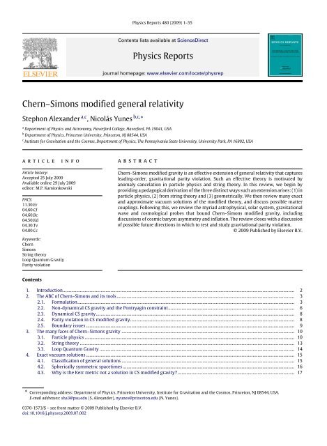
S. Alexander, N. Yunes / Physics Reports 480 (2009) 1–55 15Asthekar and Balachandran [70] noted that this ambiguity can be related, as in YM theory, to the possibility of adding tothe Einstein–Hilbert action the termS θ =iθ ∫d 4 x ∗ R R, (83)32π 2which is essentially the CS correction to the action when the scalar field ϑ = θ is constant and pulled out of the integral. Inthis sense a CS-like term arises naturally in LQG due to the requirement that wavefunctions, and thus physical observables,be invariant under large gauge transformations.But the θ-anomaly is not quite the same as CS modified gravity. After all, the above analysis is more reminiscent to thechiral anomaly in particle physics, discussed in Section 3.1. Recently, however, the connection between LQG and CS modifiedgravity has been completed, along a bit of an unexpected path. Taveras and Yunes [71] first investigated the possibility ofpromoting the Barbero–Immirzi (BI) parameter to a scalar field. This parameter is another quantization ambiguity parameterthat arises in LQG and determines the minimum eigenvalue of the discrete area and discrete volume operators [72]. At aclassical level, the BI parameter is a multiplicative constant that controls the strength of the dual curvature correction in theHolst action [69]. Taveras and Yunes realized that when this parameter is promoted to a field one essentially recovers GRgravity in the presence of an arbitrary scalar field at a classical level.Although the Holst action is attractive from a theoretical standpoint since it allows a construction of LQG in eitherAshtekar or Barbero form, this action has also been shown to lead to torsion and parity violation when one couples fermionsto the theory [73–75]. This issue can be corrected, while still allowing a mapping between GR and the Barbero–Ashtekarformalism, by adding to the Holst action a torsion squared term, essentially transforming the Holst term to the Nieh–Yaninvariant [76]. When one couples fermions to the Nieh–Yan modified theory, then the resulting effective theory remainstorsion free and parity preserving [77].Inspired by the work of Taveras and Yunes [71], Mercuri [78,79] and Mercuri and Taveras [80] considered the possibilityof promoting the BI parameter to a scalar field in the Nieh–Yan corrected theory. As in the Holst case, they found that the BIscalar naturally induces torsion, but this time when this torsion is used to construct an effective action they found that oneunavoidingly obtains CS modified gravity. In particular, one recovers Eq. (3) with ϑ = [3/(2κ)] 1/2 ˜β, with ˜β the BI scalarand α = 3/(32π 2 ) √ 3κ, while the scalar field action becomes Eq. (4) with β = 1 and vanishing potential.4. Exact vacuum solutionsOne of the most difficult tasks in any alternative theory of gravity is that of finding exact solutions, without the aid ofany approximation scheme. In the context of string theory, Campbell, et al. [23] showed that certain line elements, suchas Schwarzschild and FRW, lead to an exact CS three-form, which thus does not affect the modified field equations. In thecontext of CS modified gravity, Jackiw and Pi [22] showed explicitly that the Schwarzschild metric remains a solution ofthe non-dynamical modified theory for the canonical choice of CS scalar. Shortly after, Guarrera and Hariton [81] showedthat the FRW and Reissner–Nordstrom line elements also satisfy the non-dynamical modified field equations with the samechoice of scalar, verifying the results of Campbell, et al. [23]. Recently, Grumiller and Yunes [35] carried out an extensivestudy of exact solutions in the non-dynamical theory for arbitrary CS scalars, with the hope to find one that could representa spinning black hole. All of these investigations concern vacuum solutions in the non-dynamical framework (β = 0), withthe coupling constant choice α = κ. We shall also choose these conventions here.4.1. Classification of general solutionsLet us begin with a broad classification of general solutions in CS modified gravity. Grumiller and Yunes [35] classified thespace of solutions, a 2-dimensional representation of which is shown in Fig. 1, into an Einstein space, E, and a CS space, CS.Elements of the former satisfy the Einstein equations, while the elements of the later satisfy the CS modified field equations.The intersection of E with CS, P := E ∩ CS, defines the Pontryagin space, whose elements satisfy both the Einstein and theCS modified field equations independently. From the above definitions we can now classify solutions in CS modified gravity.Elements in P are GR solutions, because they satisfy the Einstein equations and possess a vanishing C-tensor and Pontryagindensity. Elements in CS \P are non-GR solutions, because they are not Ricci-flat but they do satisfy the Pontryagin constraintand the CS modified field equations.A full analytic study of exact solutions has been possible only regarding spacetimes with sufficient symmetries that allowfor the modify field equations to simplify dramatically. For such scenarios, however, the search for CS GR solutions have leadmostly to either Minkowski space or the Schwarzschild metric. This can be perhaps understood by considering the vacuumsector of P , where the C-tensor becomesC ab | Rab =0 = v cd∗ R d(ab)c = v cd∗ C d(ab)c = 0, (84)where C abcd and ∗ C are the Weyl tensor and its dual respectively [Eqs. (27) and (28)]. Such a condition implies the Weyltensor must be divergenceless via the contracted Bianchi identities, which leads to three distinct possibilities:(1) The (dual) Weyl tensor vanishes. In vacuum, elements of P are also Ricci flat, so this possibility leads uniquely toMinkowski space.

16 S. Alexander, N. Yunes / Physics Reports 480 (2009) 1–55Fig. 1. Space of solutions of Einstein gravity E and CS modified gravity CS. In this figure, we have set 2κ = 1 for simplicity of presentation.(2) The covariant acceleration of ϑ vanishes. Such a restriction imposes strong constraints on the geometry (cf. e.g. [42]),leading either to flat space or to the existence of a null Killing vector.(3) The contraction of the covariant acceleration and the dual Weyl tensor vanishes.Elements of P are very special, possessing a large number of symmetries and Killing vectors. On the other hand, elementsof CS \ P cannot possess too many symmetries, which explains why it has been so difficult to find them.4.2. Spherically symmetric spacetimesConsider first the most general, spherically symmetric spacetime, whose metric can be decomposed as the warpedproduct of two 2-dimensional metrics [82,83]: a Lorentzian one g αβ (x γ ) (α, β, . . . = t, r) with some coordinates x γ ; and themetric on the 2-sphere Ω ij (x i ) (i, j, . . . = θ, φ) with some coordinates x i . Such a line element can be written in the following2 + 2 form:ds 2 = g αβ (x γ ) dx α dx β + Φ 2 (x γ ) dΩ 2 S 2 , (85)where dΩ 2 S 2 is a line element of the round 2-sphere and the warped factor is the square of the scalar field Φ(x γ ), often called‘‘areal’’ radius.A spherically symmetric line element [eg. Eq. (85)] always leads to a vanishing Pontryagin density, ∗ R R = 0, and to adecoupling of the modified field equations [35]:R ab = 0, C ab = 0. (86)For the metric in Eq. (85), the only non-vanishing components of these tensors are R αβ , R ij and C αi , provided ϑ belongs tothe generic family [35,34]ϑ = F(x γ ) + Φ(x γ ) G(x i ). (87)In the non-dynamical framework, these results imply that spherically symmetric line elements are always pushed to P .Similar conclusions also hold for spherically symmetric line-elements in non-vacuum spacetimes.In the dynamical framework, one must also solve the evolution equation for the CS scalar, which here becomes a wavelikeequation without a source. In the absence of a potential, this wave-like equation need not necessarily have well-defineddecaying solutions that will lead to finite energy contained in the scalar field. If this is the case, the scalar field is forced tobe a constant, which reduces the modified theory to GR.The study of spherically symmetric line elements naturally leads to the study of Birkhoff’s theorem in CS modifiedgravity. This theorem states that the most general spherically symmetric solution to the vacuum Einstein equations is theSchwarzschild line element. For spherically symmetric line elements and the CS scalar of Eq. (87), the non-dynamical CSmodified field equations decouple and the C-tensor identically vanishes, which suffices to guarantee that Birkhoff’s theoremstill holds in the non-dynamical formulation [34].In spite of the clear persistence of Birkhoff’s theorem in the non-dynamical formulation, this theorem does not in fact holdin the dynamical framework. In this scheme, the dynamical field equations contain a scalar-field stress–energy contributionthat will unavoidingly lead to non-vacuum (i.e. hairy) solutions. Due to the presence of such a dynamical scalar field,spherical symmetry need not lead to staticity, and in fact, spherically symmetric spacetimes will in general be dynamical.Static solutions are, however, still present in dynamical CS modified gravity provided the CS scalar is a constant [84].The study of the spherically symmetric spacetimes in CS modified gravity leaves us with two important lessons:• The existence of specific solutions depends sensitively on the choice of the scalar field.• The satisfaction of the Pontryagin constraint is a necessary but not a sufficient condition for the C-tensor to vanish.In fact, it is simple to construct a CS scalar, such as a trigonometric function of spacetime, and show that for such a scalarthe C-tensor does not vanish, thus rendering the Schwarzschild metric not a solution of CS modified gravity, in spite of thevanishing of the Pontryagin density.

S. Alexander, N. Yunes / Physics Reports 480 (2009) 1–55 174.3. Why is the Kerr metric not a solution in CS modified gravity?Consider the Kerr metric in Boyer–Lindquist coordinates (t, r, θ, φ):ds 2 = − ∆ − a2 sin 2 ΘΣdt 2 − 4aMr sin2 Θdtdφ + (r 2 + a 2 ) 2 − a 2 ∆ sin 2 Θsin 2 Θdφ 2 + Σ ΣΣ∆ dr 2 + ΣdΘ 2 (88)where Σ = r 2 + a 2 cos 2 Θ and ∆ = r 2 + a 2 − 2Mr. When CS modified gravity was proposed, Jackiw and Pi [22] realizedthat the Kerr metric would not be a solution of the modified theory because the Pontryagin density is not vanishing:∗ R R = 96aM 2 rΣ 6 cos Θ ( r 2 − 3a 2 cos 2 Θ ) ( 3r 2 − a 2 cos 2 Θ ) . (89)This statement is also true in the dynamical frameworks, because the Pontryagin density will induce a non-constant CS scalarthat will lead to a non-vanishing C-tensor. One can show that the parity-odd quantity in Eq. (89), is also non-vanishing forthe Kerr–Newman and Kerr-NUT spacetimes [81,35], but it is is satisfied in certain interesting physical limits, namely a → 0(the Schwarzschild limit) and M → 0 (the pp-wave limit).Just because the Kerr metric is not a solution in CS modified gravity does not imply that a rotating BH solution is absent inthe modified theory. Modifications of the Kerr metric that do satisfy the CS modified field equations can be obtained be eitherconsidering approximate solutions or by studying the dynamical framework. For example, in the far field limit, M/r ≪ 1,the Pontryagin constraint is satisfied to O(M/r) 3 and approximate modified solutions can be derived. On the other hand,in the dynamical formalism equation (89) serves as a source term that drives the evolution of the CS scalar, which in turnsources corrections in the metric [84].An example of the latter can be found in the quantum-inspired studies of Campbell [85,86,24], Reuter [87] andKaloper [88]. For example, in [85,87], φ F ∗ ab F ab is added to the Einstein–Maxwell–Klein–Gordon action, with φ a scalar(axion) field and F ab the photon strength field tensor. The equations of motion for the scalar field acquire a source (theexpectation value of a chiral current), when one treats the photon quantum mechanically. Upon accounting for the oneloopfluctuations of the four-vector potential [89,90], one essentially finds Eq. (21), which on a Kerr background can besolved to find [87]φ = 5 ( )α a cos θ M3+ O . (90)8 β M r 2 r 3The scalar field presents a r −2 fall-off and a dipolar structure, identical to the Kalb–Ramond axion [85]. This field leads toa non-trivial C-tensor that corrects the Kerr line element, thus disallowing this metric as a solution of the modified theory.Nonetheless, the axion in Eq. (90) could (and has) been used to construct correction to the Kerr metric [84], as we shalldiscuss in Section 5.4.4. Static and axisymmetric spacetimesLet us now consider static and axisymmetric line elements in vacuum and in the non-dynamical framework. Bothstationary and static, axisymmetric spacetimes possess a timelike (∂ t ) a and an azimuthal ( ∂ φ) aKilling vector, but thedifference is that static metrics contain no cross-terms of type dtdφ. The most general such metric is diffeomorphic to [20]ds 2 = −V dt 2 + V −1 ρ 2 dφ 2 + Ω 2 ( dρ 2 + Λdz 2) , (91)where V(ρ, z), Ω(ρ, z) and Λ(ρ, z) are undetermined functions of two coordinates, ρ and z.Consider first the canonical choice of CS scalar. The modified field equations once more decouple, as in Eq. (86) and thespherically symmetric case, which implies all static and axisymmetric solutions are elements of P , identically satisfying thePontryagin constraint. Due to this, we can make choose Λ = 1 and put the metric into Weyl class [20,42]:ds 2 = −e 2U dt 2 + e −2U [ e 2k (dρ 2 + dz 2 ) + ρ 2 dφ 2] , (92)where U(ρ, z) and k(ρ, z) replace the functions V and Ω.The vanishing of the Ricci tensor reduces to∆U = 0, k ,ρ = ρ(U 2 ,ρ − U 2 ,z ), k ,z = 2ρU ,ρ U ,z , (93)where ∆ = ∂ 2 /∂ρ 2 + 1/ρ∂/∂ ρ + ∂ 2 /∂z 2 is the flat space Laplacian in cylindrical coordinates. The function k can be solvedfor through a line integral once U is determined [42].The vanishing of the C-tensor reduces to the vanishing of the contraction of the dual Weyl tensor and the covariantacceleration of the CS coupling field. For a canonical ϑ, one finds [35]Ɣ t ρt ∗ C t(ab)ρ + Ɣ t zt ∗ C t(ab)z = 0, (94)which leads to a set of nonlinear PDEs for U, in addition to the Laplace equation of Eq. (93).

18 S. Alexander, N. Yunes / Physics Reports 480 (2009) 1–55The set of equations imposed by Eq. (86) can be solved exactly, yielding either flat space, the Schwarzschild solution orthe following two solutions:ds 2 = − 1 z dt2 + zdz 2 + z 2 (dρ 2 + ρ 2 dφ 2 ) (95)and)( 2mds 2 = −z− 1( 2mdt 2 +z− 1) −1dz 2 + z 2 (dρ 2 + sinh 2 ρ dφ 2 ). (96)These solutions, however, contain undesirable, non-physical features, such as the existence of a naked singularity at z = 0[Eq. (95)], or the existence of a spacelike Killing vector k a = (∂ t ) a in the ‘‘outside’’ region z > 2m [Eq. (96)].The above results can also be obtained by noticing that the spatial sector of C ab reduces identically to the 3-dimensionalCotton–York tensor for static and axisymmetric line elements, which by the decoupling of the field equations must vanishexactly [35]. This implies the metric must be spatially conformally flat. Lukács and Perjés [91] have shown that such solutionsto the Einstein equations reduce to Minkowski, Schwarzschild or the line elements of Eqs. (95) and (96), as described above.The above results hold for any CS scalar in the familyϑ = ϑ 1 (t, ρ, z) + ϑ 2 (ρ, z, φ). (97)For even more general CS scalars, as would arise, for instance, in the dynamical formulation, the modified field equationsdo not necessarily decouple and, thus, new and interesting solutions could arise. Unfortunately, when this is the case, thesystem of partial differential equations becomes too difficult to study analytically and has not really been analyzed in detail.4.5. Stationary and axisymmetric spacetimesNow consider stationary and axisymmetric spacetimes [42]:ds 2 = −V (dt − wdφ) 2 + V −1 ρ 2 dφ 2 + Ω 2 ( dρ 2 + Λdz 2) , (98)where V , Ω, Λ and w depend on ρ and z, with the latter identified with angular velocity of rotation about the Killing axis.Let us first consider the canonical choice of CS scalar, for which the modified field equations decouple once more. TheEinstein equations can be used to set Λ to unity and put the line element in Lewis–Papapetrou–Weyl form [42]ds 2 = −e 2U (dt − wdφ) 2 + e −2U [ e 2k (dρ 2 + dz 2 ) + ρ 2 dφ 2] , (99)where U and k replace V and Ω.The vanishing of the Ricci tensor reduces to a set of partial differential equations similar to Eq. (93), with a non-trivialsource that depends on w and an additional equation for this function. The vanishing of the C-tensor, however, does notlead to a vanishing Cotton–York tensor, and thus, it does not necessarily imply spatial conformal flatness. Grumiller andYunes [35] have argued that it seems unlikely that other non-trivial and physically interesting solutions besides the staticones could arise, because R ab = 0 and C ab = 0 is a strongly over-constrained differential system. This is an example ofhow the non-dynamical theory can lead to an overconstrained system of equations when searching for physically relevantsolutions, but a strict proof remains elusive.The argument presented above holds for any ϑ in the familyϑ = t µ + φ ν , (100)with constants µ and ν. When the CS coupling is not of the form of Eq. (100), then the field equations do not decouple, thearguments presented above do not hold and the system become more difficult to analyze analytically.In the non-dynamical framework, another route to exact solutions for generic CS scalars is through the Pontryaginconstraint. For axisymmetric spacetimes, ∗ R R ≠ 0, and this leads to a complicated set of partial differential equationsfor w, U and k. Solutions of ∗ R R = 0 have been found to be of Petrov type II [35], which correspond to the Van Stockumclass [42]ds 2 = ρΩdt 2 − 2ρdtdφ + 1 √ ρ(dρ 2 + dz 2) , (101)where Ω = Ω(ρ, z) is arbitrary and there is no dφ 2 component.The reduced Van-Stockum class of metrics leads to a complete decoupling of the modified field equations, except forthe dt 2 component. The vanishing of the C-tensor can be achieved if ϑ = ϑ(ρ, z), while the dt 2 component of the fieldequations can be solved to findΩ = c, ϑ = ϑ(ρ, z), (102)Ω = c +d √ ρ, ϑ = 2 3√ ρ z + ˜ϑ(ρ), (103)

S. Alexander, N. Yunes / Physics Reports 480 (2009) 1–55 19where c and d are constants. Eq. (102) is non-flat, possessing a non-vanishing Riemann tensor and a third Killing vectort∂ t − φ∂ φ + ct∂ φ , but it satisfies R ab = 0 and C ab = 0 independently (i.e. it belongs to P ). Eq. (103) is Riemann and Riccinon-flat (R abcd ≠ 0, R ab = −C ab ≠ 0), belonging to CS \ P . This last solution can be interpreted as a BH solution in themathematical sense only, provided Ω vanishes for some ρ and a Killing horizon appears, because it allows for closed timelikecurves outside the Killing horizon [35].We see then that physically relevant, stationary and axisymmetry, exact solutions have not been found in non-dynamicalCS gravity, even when considering generic CS scalars fields. We say relevant solutions here, because non-physical oneshave been found, but they either contain naked singularities or closed time-like curves. In fact, as an example of the latter,recently [92] has shown that the Godel line element ds 2 = a 2 (dt 2 − dx 2 + e 2x dy 2 /2 − dz 2 + 2e x dtdy), which is a subclass ofthe metrics considered in this section, satisfies the non-dynamical modified field equations with the CS scalar ϑ = F(x, y),for some arbitrary function F. Such a solution is of class P because the C-tensor automatically vanishes with such choices.All evidence currently points at the modified field equations being over-constrained by the Pontryagin condition and thefield equations. Although this evidence is strong, no proof currently exists to guarantee that no solution can be found.Moreover, in the dynamical framework, the relaxation of the Pontryagin constrain suffices to allow the existence of Kerr-likesolutions [84].4.6. pp-waves and boosted black holesConsider line elements that represent exact gravitational wave solutions (pp-waves [93]):ds 2 = −2dvdu − H(u, x, y)du 2 + dx 2 + dy 2 , (104)where H is the only free function of u, x and y. The Aichelburg–Sexl limit [94] of various BHs is in fact an example of sucha line element. This limit consists of ultrarelativistically boosting the BH, while keeping its energy finite, by simultaneouslytaking the mass to zero as the boost speed approaches that of light [95,96].For such metrics, the Pontryagin constraint vanishes identically, which at first seems in contradiction with the results ofJackiw and Pi [22], who showed that generic linear GW perturbations lead to ∗ R R = O(h 2 ). In fact, these two results areactually consistent, because the line elements considered here and in [22] are intrinsically different and cannot be relatedvia diffeomorphism. The fact that the Pontryagin density vanishes for the metric of Eq. (104) is related to the fact that theCS velocity field v a = ∂ a ϑ is a null Killing vector v a v a = 0 for such spacetimes [35].The modified field equations decouple, except for the du 2 component. Consider first solutions that live in P [ Eq. (86)],which require the vanishing of the C-tensor, thus forcingϑ = λ(u)v + ˜ϑ(u, x, y). (105)The vanishing of the Ricci tensor forces∆H = 0, (106)2H ,yy ˜ϑ ,xy = H ,xy ( ˜ϑ ,yy − ˜ϑ ,xx ). (107)Therefore, for any H that solves the Laplace equation in Eq. (106), we can find a ˜ϑ such that Eq. (107) is also satisfied. Such ascheme allows one to lift any pp-wave solution of the vacuum Einstein equations to a pp-wave solution of non-dynamicalCS modified gravity of class P through a choice of ϑ that satisfies Eqs. (105) and (107) [35].Now consider solutions that live in CS \ P . All non-uu components of the modified field equations decouple, and thusthe vanishing of the C-tensor is satisfied by scalar field of the form of Eq. (105). Choosing λ(u) = 0 for simplicity, we findthat the uu component of the modified field equations reduces to a third order PDE(1 + ˜ϑ ,y ∂ ,x − ˜ϑ ,x ∂ ,y )∆H = ( ˜ϑ ,xx − ˜ϑ ,yy )H ,xy − (H ,xx − H ,yy ) ˜ϑ ,xy . (108)Simplifying this scenario further by choosing ˜ϑ = a(u)x + b(u)y + c(u), Eq. (108) reduces to the Poisson equation ∆H = f ,whose source satisfies a linear first order PDE bf ,x − af ,y − f = 0, with general solution [assuming b(u) ≠ 0]f (u, x, y) = e x/b(u) φ [a(u)x + b(u)y] (109)where φ is an arbitrary function. With such a source and two supplementary boundary conditions, we can now solve thePoisson equation and specify the full modified pp-wave solution [35]. Thus, generic CS \ P solutions do exist in nondynamicalCS modified gravity and can be found via the algorithm described above.4.7. Non-axisymmetric solutions and matterIn the non-dynamical framework, axisymmetry seems to limit the existence of solutions for a certain class of couplingfunctions. However, if either axisymmetry, the non-dynamical behavior of ϑ or the vacuum content assumption is relaxed,it is possible that solutions in fact do exist.Consider losing axisymmetry first. The general idea here is to add new degrees of freedom in the metric that couldcompensate for the overconstraining of the decoupling of the modified field equations. Such an idea is in fact inspiredfrom approximate far-field solutions found in non-dynamical modified CS gravity, which indeed require the presence of

20 S. Alexander, N. Yunes / Physics Reports 480 (2009) 1–55additional, non-vanishing, gravitomagnetic metric components. Up to the writing of this review, the only attempts to findsuch solutions have failed [35], due to the incredible complexity of the differential system.Consider next spacetimes with matter content. The Kerr BH is a ‘‘vacuum’’ solution in GR, but it does possess adistributional energy momentum tensor [97]. Moreover, in string theory and cosmology [28], CS modified gravity arisesfrom matter currents, so the inclusion of such degrees of freedom might in principle be important. In the dynamical scheme,for example, one could lift any GR solution to a solution of CS modified gravity by requiring thatR ab − 1 2 g abR = 8πT matab , (110)C ab = 8πT ϑ ab , (111)where T matabstands for the stress–energy of matter degrees of freedom (such as the distributional one associated with theKerr solution), while T ϑ abis the energy–momentum of the CS coupling. One would now have to solve the system of PDEsassociated with Eq. (111) for the background which satisfies Eq. (110). Such a task, however, would imply also solving theequation of motion for the CS scalar, thus reducing this analysis to the study of exact solutions in dynamical CS modifiedgravity, which has not yet been performed.5. Approximate vacuum solutionsApproximate schemes have been employed to solve the CS modified field equations in different limits. The first attemptalong these lines was that of Alexander and Yunes [32,7], who performed a far-field, PPN analysis of non-dynamical CSmodified gravity (α = κ, β = 0) with canonical ϑ. This study was closely followed by that of Smith, et al. [37] who carriedout a far-field investigation of non-dynamical solutions representing the gravitational field outside a homogeneous, rotatingsphere, taking careful account of the matching between interior and exterior solutions. Konno, et al. [98] investigated theslow-rotation limit of stationary and axisymmetric line elements in non-dynamical CS modified gravity with non-canonicalCS scalar fields. Finally, gravitational wave solutions of CS modified gravity have been studied by a number of authors, bothin Minkowski spacetime and in an FRW background [22,28,31,29,33,36]. The last two set of studies were carried out in thenon-dynamical formalism with the choices α = κ and β = 0. Little is known about GW propagation or generation indynamical CS modified gravity, although early efforts are being directed on that front [84,99].5.1. Formal post-Newtonian solutionThe PN approximation has seen tremendous success to model full general relativity in the slow-motion, weaklygravitating regime (for a recent review see [100]). This approximation is used heavily to study Solar System tests ofalternative theories of gravity in the PPN framework, as well as to describe gravitational waves from inspiraling compactbinaries, which could be observed in gravitational wave detectors in the near future. For these reasons, it is instructive tostudy the PN expansion of CS modified gravity, before submerging ourselves in other approximate solutions.The PN approximation is essentially a slow-motion and weak-gravity scheme in which the field equations of some theoryare expanded and solved perturbatively and iteratively. As such, this scheme makes use of multiple-scale perturbationtheory [101–104], where the perturbation parameters are the self-gravity of the objects (an expansion in powers of Newton’sconstant G) and their typical velocities v (an expansion in inverse powers of the speed of light). For example, matter densitiesρ are dominant over pressures p and specific energy densities Π, while spatial derivatives are dominant over temporal ones.The PN framework also requires the presence of external matter degrees of freedom, i.e. bodies that are self-gravitatingand slowly-moving. Such objects can be described in a point-particle approximation [100], or alternatively with a perfectfluid stress–energy tensor [105]:T ab = (ρ + ρΠ + p) u a u b + pg ab , (112)where u a is the object’s four-velocity. In GR, the internal structure of the gravitating objects can be neglected to rather largePN order [106], and thus one can effectively take the radius of the fluid balls to zero, which reproduces the point-particleresult. This statement is that of the effacing principle [106], which is the view we shall take in the next section when westudy CS modified gravity in the PPN framework. However, care must be taken, since the effacing principle need not holdin alternative theories of gravity. In fact, as we shall see later on, the effacing principle must be corrected in CS modifiedgravity due to modifications to the junction conditions [107–113,21,114].Perturbation theory, and thus the PN approximation, requires the use of a specific background and coordinate system.In the traditional PN scheme, one linearizes the field equation with the metric g ab = η ab + h ab , where η ab is the Minkowskibackground, since cosmological effects are usually subdominant. Moreover, a Lorentz gauge is usually chosen h ba,a = h ,b /2,which allows one to cast the field equations as a wave equation with non-trivial, non-linear source terms. One can showthat to first order in the metric perturbation, the linearized CS modified field equations in the non-dynamical formalism,with canonical CS scalar and in the Lorentz gauge, can be written as [32,7](□ η H ab = −16π T ab − 1 )2 g abT + O(h) 2 , (113)

S. Alexander, N. Yunes / Physics Reports 480 (2009) 1–55 21where the superpotential H ab captures the CS modification to the PN expansion to the modified field equations and it isgiven byH ab := h ab + ˙ϑ ˜ɛ 0cd (ah b)d,c , (114)where ˜ɛ abcd stands for the Levi-Civita tensor density. The 00 component, the symmetric spatial part and the trace of thesuperpotential are equal to that of the metric perturbation, because the Levi-Civita symbol forces the CS correction to vanish.The formal solution to the modified field equations then reduces toH ab = −16π □ −1η(T ab − 1 2 g abT)+ O(h) 2 , (115)where the inverse D’Alembertian operator stands for a Green function integral. This formal solution is in fact identical tothat of the PN expansion of GR in the limit ˙ϑ → 0.This formal solution can also be cast into a more practical form by perturbatively solving for the metric perturbation [32,7]. Let us then make the ansatzwhere h (GR)abh ab = h (GR)ab+ ˙ϑ ζ ab + O(h) 2 , (116)h (GR)abis the GR solution, which is ϑ-independent and satisfies(:= −16π □ −1ηT ab − 1 2 g abT), (117)and where ζ ab is an unknown function that is first order in ˙ϑ. When we combine Eqs. (115), (114) and (116) we find(ζ ab + ˙ϑ ˜ɛ 0cd (aζ b)d,c = 16π ˜ɛ 0 c d (a∂ c □ −1η T b)d − 1 )2 g b)dT , (118)which can be solved for to find(ζ ab = 16π ˜ɛ 0 c d (a∂ c □ −1η T b)d − 1 )2 g b)dT , (119)where we have neglected terms second order in ϑ. The metric perturbation then reduces to(h ab = −16π □ −1η T ab − 1 )2 η abT + 16π ˙ϑ ˜ɛ kli □ −1η(δ i(a T b)l,k − 1 )2 δ i(aη b)l T ,k , (120)where i, j, k stand for spatial indices only.5.2. Parameterized post-Newtonian expansionSolar system tests of alternative theories of gravity are best performed within the PPN framework. This framework wasfirst proposed by Eddington, Robertson and Schiff [115,116], but it matured with the work of Nordtvedt and Will [117–120](for a review see e. g. [115]). PPN theory proposes the construction of a model-independent super-metric that representsthe PN approximate solution to a family of gravity theories, parameterized by PPN parameters. Solar system experimentscan then measure these parameters, thus selecting a particular member of this family. Currently, many of these parametershave been experimentally determined with tight error bars, all of which are consistent with GR [121].The PPN framework allows for tests of alternative theories of gravity through such PPN parameters. Given an alternativetheory, one must first construct its PN solution and then compare it to the PPN super-metric. Through this comparison, onecan read off how the PPN parameters depend on fundamental parameters of the alternative theory. But since PPN parametershave been experimental constrained, one can propagate these constraints to the fundamental parameters of the alternativetheory under consideration, thus obtaining an automatic Solar System test.Solar System tests in the PPN framework require the PN solution to the modified field equations. In this framework,however, it is not sufficient to leave the solution expressed in terms of the inverse D’Alembertian operator, but instead itmust be parameterized in terms of PPN potentials, which are simply Green function integrals over the stress energy tensor.Moreover, the PN expansion must be carried out to slightly different orders in v for different components of the metric, soas to obtain a consistent Lagrangian formulation of the theory. 5 In the PPN framework, it suffices to compute g 00 to O(v 4 ),g 0i to O(v 3 ) and g ij to O(v 2 ). Finally, the Lorentz gauge differs slightly from the PPN gauge, related via an infinitesimal gaugetransformation, where the latter is perturbatively defined via [115]h jk, k − 1 2 h ,j = O(4), h 0k, k − 1 2 hk k,0 = O(5), (121)5 For example, such order counting is necessary in order to calculate the gravitational deflection of light consistently to first order.

22 S. Alexander, N. Yunes / Physics Reports 480 (2009) 1–55where i, j, k stand for spatial indices only in the remaining of this section, h k k is the spatial trace of the metric perturbationand the symbol O(A) stands for terms of O(ɛ A ), with ɛ the standard PN expansion parameter of O(1/c) [32,7].With this machinery at hand, we can now perturbatively expand the trace-reversed CS modified field equations. For theremaining of this chapter, we shall concentrate on the non-dynamical formalism of CS modified gravity, with the canonicalchoice of CS scalar. Expressions for the linearized Ricci and C-tensors to O(4) in an arbitrary gauge and for generic ϑ arelong and unilluminating, so we shall not present them here, but they can be found in [37]. On the other hand, in the PPNgauge and with the canonical choice for ϑ, the linearized Ricci tensor becomesR 00 = − 1 2 ∇2 h 00 − 1 2 h 00,ih 00, i + 1 2 hij h 00,ij + O(6),R 0i = − 1 2 ∇2 h 0i − 1 4 h 00,0i + O(5),R ij = − 1 2 ∇2 h ij + O(4), (122)while the linearized C-tensor is given byC 00 = O(6),C 0i = − 1 ˙ϑ ˜ɛ 0kl i∇ 2 h 0l,k + O(5),4C ij = − 1 ˙ϑ ˜ɛ 0kl (i∇ 2 h j)l,k + O(4), (123)2where ∇ = η ij ∂ i ∂ j is the flat-space Laplacian. As in Section 5.1, we find two distinct corrections due to the CS modification:one to the transverse-traceless part of the spatial metric and the other to the vector metric perturbation.Let us now solve the linearized CS modified field equations iteratively and perturbatively. To O(2), the 00 component ofthe metric is not modified by the C-tensor and the field equation becomes∇ 2 h 00 = −8πρ, (124)because T = −ρ. Eq. (124) is the Poisson equation, whose solution in terms of PPN potentials ish 00 = 2U + O(4), (125)where U is the Newtonian potential [32,7]. We shall not present these potentials here, but they can be found in [115].To this same order, the 0i component does not provide any information, while the ij sector leads to the following fieldequations:∇ 2 h ij + ˙ϑ ˜ɛ 0kl (i∇ 2 h j)l,k = −8πρδ ij , (126)where δ ij is the Kronecker delta. This equation can be rewritten in terms of the superpotential of Section 5.1 as∇ 2 H ij = −8πρδ ij , (127)whose solution is [32,7]H ij = 2Uδ ij + O(4). (128)Following the same procedure as in Section 5.1, we can use the decomposition of Eq. (116) to find thatζ ij + ˙ϑ ˜ɛ 0kl (iζ j)l,k = 0. (129)The second term on the left-hand side of Eq. (129) is a second order correction in ˙ϑ and can thus be neglected, which thenrenders h ij = H ij to O(2), where the latter is given in Eq. (128). The physical reason why the CS modification does notcorrect the spatial sector of the metric is related to the source studied here, together with the PPN gauge. In fact, we shallsee in Section 5.6 that when one studies gravitational wave propagation in vacuum, the spatial sector of the metric is indeedmodified. Moreover, if we were to study the O(4) corrections to the spatial sector of the metric, we would probably findnon-vanishing CS corrections, but such a study has not yet been carried out.To next order, O(3), the only relevant field equations are related to the gravitomagnetic sector of the metric. The fieldequations become [32,7]∇ 2 h 0i + 1 2 h 00,0i + 1 ˙ϑ ˜ɛ 0kl i∇ 2 h 0l,k = 16πρv i , (130)2which with the lower-order solution of Eq. (125) and the superpotential of Eq. (114) becomes∇ 2 H 0i + U ,0i = 16πρv i , (131)

S. Alexander, N. Yunes / Physics Reports 480 (2009) 1–55 23whose solution isH 0i = − 7 2 V i − 1 2 W i, (132)where V i and W i are PPN vector potentials. Combining Eq. (114) with Eq. (116), we can solve Eq. (132) to find [32,7]h 0i = − 7 2 V i − 1 2 W i + 2 ˙ϑ (∇ × V) i + O(5), (133)where (∇ × A) i = ˜ɛ ijk ∂ j A k is the standard curl operator of flat spaceFinally, to next order, O(4), we need only analyze the 00 component of the modified field equations. Since the 00component of the C-tensor does not contribute to the field equations to this order, the modified field equations reduceexactly to those of GR, as also does their solution. We therefore find that the PPN solution to the CS modified field equationsis given byg 00 = g (GR)00+ O(6),g 0i = g (GR)0i+ 2 ˙ϑ (∇ × V) i + O(5),g ij = g (GR)ij+ O(4), (134)where g (GR)abis the PPN solution of GR. This solution in fact satisfies the Pontryagin constraint ⋆ RR = 0 to leading orderbecause the contraction of the Levi-Civita symbol with two partial derivatives vanishes. Thus, the equations of motion forthe fluid can be obtained directly from the covariant derivative of the stress–energy tensor (the strong equivalence principleholds).By comparing this PPN solution to the super-metric of the PPN framework, we can now read off the PPN parameters ofCS gravity [32,7]. Doing so, one finds that all PPN parameters of CS gravity are identical to those of GR (γ = β = 1, ζ = 0and α 1 = α 2 = α 3 = ξ 1 = ξ 2 = ξ 3 = ξ 4 = 0), except for the new term in g 0i . This CS correction cannot be mimicked byany standard PPN parameter, and thus, in order to model parity-violating theories an additional PPN parameter χ must beintroduced, namelyg 0i = g (PPN)0i+ χ (M∇ × V) i , (135)where we have multiplied the curl operator by the total mass M, in order to make χ a proper dimensionless parameter. InCS modified gravity, this parameter is simply χ = 2 ˙ϑ/M.Canonical CS modified gravity can then be tested by experimentally constraining χ, which thus directly places aconstraint on the canonical CS scalar ˙ϑ = 1/µ. The only requirement for such a contribution to be non-vanishing is thatthe PPN vector potential V i be non-vanishing. This is satisfied by non-static sources (i.e. objects that are either moving orspinning relative to the PPN rest frame). Just because the correction to the gravitomagnetic sector of the metric is nonvanishing,however, does not imply that physical observables, such as the Lense–Thirring effect, will also be corrected. Infact, as we shall see in Section 7.1, for such corrections to emerge, the curl of the gravitomagnetic correction to the metricmust be non-vanishing, which holds only for moving point particles.A caveat should be discussed at this point. As we already alluded to, the point-particle approximation holds in GR formany sources, such as black holes, neutron stars or other regular stars, because the effacing principle holds and Birkhoff’stheorem also holds. In CS gravity, however, the former does not necessarily hold and the junction conditions are modified.One should then also be aware that a homogeneous solution to the linearized field equations might be lacking from thisanalysis. Such a solution is most likely oscillatory in nature and would not affect the average behavior of the correction,probably acquiring importance only when the latter vanishes. In the next section we shall see how such a boundary solutionarises and contributes significantly for spinning bodies, for which the homogeneous correction to the Lense–Thirring effectvanishes.5.3. Rotating extended bodies and the gravitomagnetic analogyThe analysis presented so far has dealt with the non-dynamical formalism, concentrating primarily on point particlesources. Approximate solutions, however, can be developed for extended objects as well. As already described, in GR theeffacing principle guarantees that for certain sources both the extended and point particle approach coincide up to ratherhigh PN order. This result somewhat relies on the junction conditions of GR, which here are modified due to the presenceof the C-tensor in the field equations. Moreover, the PN scheme is not the only formalism in which far field solution can beinvestigated. In particular, the gravitoelectromagnetic analogy [122,123] is also useful to obtain far field solutions, since itallows one to use machinery from the theory of electromagnetism.Smith, et al. [37] performed the first detailed analysis of rotating, extended objects in CS modified gravity in thegravitoelectromagnetic scheme, modeled via the stress–energy tensorT ab = 2t (a J b) − ρt a t b , (136)

24 S. Alexander, N. Yunes / Physics Reports 480 (2009) 1–55where the current J a := (−ρ,⃗ J) and ta = [1, 0, 0, 0] is a time-like unit vector. 6 Such a choice of stress–energy is equivalentot that of a pressureless perfect fluid in the limit as the fluid balls tend to particles. Moreover, Smith, et al. [37] focused onthe dynamical formulation of CS modified gravity, with the conventions α = −l/3 and β = −1. Such a study is forbiddenin the non-dynamical formalism, because the Pontryagin constraint does not allow for rotating solutions. In the dynamicalscheme, however, such solutions are allowed, provided the Pontryagin density is balanced by the dynamics of the scalarfield.In spite of working in the dynamical theory, Smith, et al. [37] chose a canonical ϑ, thus implicitly treating this field as nondynamical.Such a choice of scalar field is formally inconsistent with dynamical CS modified gravity, since the non-vanishingPontryagin constraint will force spatial variations on ϑ. Nonetheless, this choice could become a good approximation, if oneis only concerned with far-field solutions. This is because, as we have shown in Eq. (89) of Section 4.3, the exterior Pontryagindensity for a rotating source scales as ∗ R R ≈ aM 2 /r 7 , which then forcesβ□ϑ = −24α aM2r 7= 8l aM2 , (137)r 7with uncontrolled remainders of O(M/r) 4 . Thus, spatial variations will induce modifications to the canonical ϑ that are atmost of O(M/r) 3 , which is beyond the order considered in this section. A full dynamical study of this problem has yet to becarried out.Let us now return to the gravitoelectromagnetic formalism, in which certain components of the metric perturbation areidentified with a four-vector potential, namelyA a := − 1 ¯h ab t b , (138)4where ¯hab is the trace-reversed metric perturbation ¯hab := h ab − 1 2 η abh and h = η ab h ab is the trace of the latter. In analogywith electromagnetism, one can now define electric and magnetic fields viaE i = ∂ i A 0 − ∂ 0 A i , B i = ɛ 0ijk ∂ j A k , (139)where i, j stand for spatial indices only. The geodesic equations can then be written in terms of these fields asF i = −mE i − 4m (v × B) i , (140)where the cross product is that of flat Euclidean space, from which one can read off the Lorentz force acceleration a i = F i /m.We can now apply this formalism to the linearized CS modified field equations. In the Lorentz gauge, A a ,a= 0, the modifiedfield equations become [37]⃗∇ · ⃗ B = 0, (141)⃗∇ × E ⃗∂⃗ B = −∂t , (142)⃗∇ · E ⃗ = 4πG(ρ + Tϑ00 (143)⃗∇ × ⃗ B −∂⃗ E∂t − 1m cs□⃗ B = 4πG ⃗ J, (144)where m cs is a characteristic mass scale defined viam cs := 2κα ˙ϑ = − 6κl ˙ϑ . (145)In the above equations, the first two arise from the definitions of the four-vector potential, while the last two (Gauss’slaw in Eq. (143) and Ampère’s law in Eq. (144)) are modified in CS modified gravity, the former arising from the timetimecomponent of the modified field equation and the latter from the gravitomagnetic sector. Smith, et al. [37] neglect T ϑ 00because they associate it with the energy density of the scalar field, which they argue must be uniform throughout the SolarSystem, not larger than the mean cosmological energy density and negligible relative to ρ. Moreover, from Eq. (15), we seethat T ϑ 00 is at least quadratic in ˙ϑ and can thus be neglected, provided 3β/(2ρµ 2 ) ≪ 1.Let us now specialize the above treatment to that of homogeneous rotating source, with mass current⃗ J = ρ[⃗ω × ⃗r]Θ(R − r), (146)where R is the radius of the rotating body, ρ is its density, ⃗ω is its angular velocity, r is the distance from the origin, and Θis the Heaviside step function. One can now use this mass current in Ampère’s law to solve this equation for A i , imposing6 Recall that indices are raised and lowered with the Minkowski metric in the far-field approximation.

S. Alexander, N. Yunes / Physics Reports 480 (2009) 1–55 25continuity and finiteness at the origin. The actual expressions for the four-vector potential can be found in [37], but itsassociated gravitomagnetic field is given by B ⃗ = BGR ⃗ + BCS ⃗ , where the GR piece is simply⎧⎪⎨(5 − 3 r )2⃗ω + 3 r 2ˆr × (ˆr × ⃗ω), r ≤ R,⃗B GR = 4πGρR2 R 2 R2 (147)15 ⎪⎩ R 3 [ ]2⃗ω + 3ˆr × (ˆr × ⃗ω) , r ≥ R,r 3while the CS correction is given by⃗B CS = 4πGρR 2 { D 1 (r) ⃗ω + D 2 (r) ˆr × ⃗ω + D 3 (r) ˆr × (ˆr × ⃗ω) } . (148)The function D 1,2,3 (r) are actually functionals of spherical Bessel functions of the first j l (x) and second y l (x) kind, givenexplicitly in [37]. Remarkably, the gravitoelectromagnetic analogy allows for a solution to the linearized modified fieldequations for an extended rotating source, which possesses both a poloidal and toroidal gravitomagnetic field. In otherwords, the metric does not only contain gravitomagnetic components co-aligned with the spin axis of the rotating extendedbody, but also along other axis, perpendicular to the plane defined by ⃗ω and ⃗r. Such terms cannot indeed be removed via acoordinate transformation since B i φ is generically non-vanishing.The solution for the metric perturbation found in the gravitoelectromagnetic analogy for extended sources differs slightlyfrom that found in the PN scheme for point particles. Some of these differences arise because in the latter the point particleswere allowed to possess non-vanishing angular and linear momentum. The main difference, however, is not due to thestress–energy tensor studied, but to the fact that extended and point particle treatments are not equivalent in CS modifiedgravity. In the former, an additional oscillatory behavior is needed, encoded in the appearance of Bessel functions, in order toguarantee continuity across the surface of the sphere. Such terms are necessary because the C-tensor modifies the junctionconditions of GR [107–113,21,114].The gravitoelectromagnetic analogy also sheds some light on the study of exact solutions to CS modified gravity, reviewedin Section 4. The CS correction to Ampère’s law, Eq. (144) changes the character of the differential system, from a first-orderone to a second-order one. Such a result is in fact expected from the structure of the modified field equations [ Eq. (18)], sincethe C-tensor depends on third-order derivatives of the metric. One then could also expect that approximate solution to CSmodified theory need not be easily obtained as deformations of GR solutions. This is because, in principle, the CS correctioncould produce dramatic changes to the dynamical behavior of the solution (i.e. the solution, for example, could be an elementof CS \ P in the nomenclature of Section 4, which would hold little resemblance to GR solutions). CS modified theory andGR, however, have both now been sufficiently tested to allow for a perturbative treatment of the modified theory, at leastin the Solar System. Whether such treatment is allowed in more non-linear, strong field scenarios remains to be studiedfurther.5.4. Perturbations of the Schwarzschild spacetimeBlack hole perturbation theory has been incredibly important in GR, leading for example to a better understanding ofsubtle issues related to BH physics and the extraction of gravitational waves in dynamic spacetimes. Moreover, through thediscovery of quasinormal ringing, new tests of GR have been proposed (see eg. [124] for a review). These accomplishmentsalone suggest a study of BH perturbation theory in CS modified gravity could lead to interesting results. Such a study wascarried out by Yunes and Sopuerta [34] in the non-dynamical formalism with α = κ and β = 0.Let us begin by introducing the basics of BH perturbation theory, as developed in GR. Consider then the followingperturbed metricg ab = ḡ ab + h ab , (149)where ḡ ab is the background Schwarzschild metric and h ab is a generic metric perturbation. Henceforth, objects associatedwith the background will be denoted with an overhead bar. The spherical symmetry of the background allows one to expandthe metric perturbation in tensor spherical harmonics, thus separating the angular i = {θ, φ} and temporal-radial µ = {t, r}dependence in the perturbed field equations and yielding a 1 + 1 PDE system. This system can be further simplified bydistinguishing between polar and axial parity harmonics: polar (axial) modes acquire a (−1) l [(−1) l+1 ] prefactor upon paritytransformations. The aforementioned simplification comes about because in GR the perturbative field equations decoupleinto two subsystem that can be classified by their parity.With these considerations in hand, we split the metric perturbation into h ab = h a + ab hp ab, where each of these pieces isdecomposed in tensor spherical harmonics: the temporal-radial sector becomesh a µν = 0,hp µν = ∑ l,mh p,lmµν = ∑ h lmµν Y lm , (150)l,mthe temporal-angular sector is given byh a µi = ∑ l,mh a,lmµi= ∑ h lmµ Slm i, h p = ∑ µih p,lmµi= ∑ p lmµ Y lmi, (151)l,ml,ml,m

26 S. Alexander, N. Yunes / Physics Reports 480 (2009) 1–55and the angular–angular sector becomesh a ij = ∑ l,mh a,lmij= ∑ l,mH lm S lmij, h p = ∑ ijh p,lmij= ∑ ( r 2 K lm Y lmijl,ml,m)+ G lm Z lmij , (152)asterisks denote components given by symmetry and where Y lm are standard scalar spherical harmonics [see [125] forconventions], Y lmiand S lmiare polar and axial vector spherical harmonics respectively, and Y lmij, Z lmijand S lmijare polar, polarand axial, tensor spherical harmonics. Vector spherical harmonics are defined for l ≥ 1 viaY lmi≡ Y lm:i, S lmj≡ ɛ j i Y lmj(153)while tensor spherical harmonics are defined for l ≥ 2 viaY lmij:= Y lm Ω ij , Z lmij:= Y lm:ij+l(l + 1)Y lm Ω ij ,2S lmij:= S lm(i:j) , (154)where Ω ij and ɛ ij are the metric and Levi-Civita tensor on the 2-sphere respectively, while colon stands for covariantdifferentiation on the 2-sphere. All metric perturbations are functions of t and r only.The perturbative field equations can be decoupled in GR in terms of complex master functions, known as theCunningham–Price–Moncrief (CPM) master function [126] and the Zerilli–Moncrief (ZM) master function [127,128]. Theformer is given byΨ lm = − r (CPMh lmλ − r,t hlm + 2 )t,rl r hlm t, (155)where λ l = (l + 2)(l − 1)/2, while the latter is given byΨ lm = r {ZMK lm + (1 + λ l )G lm + f [fh lmrr− rK lm,r− 2 ]}1 + λ l Λ l r (1 + λ l)p lmr, (156)where f = 1 − 2M/r is the Schwarzschild factor and Λ l = λ l + 3M/r.The perturbative field equations can be written in terms of these master function, obtaining the so-called masterequations[]−∂ 2 t 2 + ∂ 2 r 2 ⋆ − V Polar/Axiall(r)Ψ lmCPM/ZM= 0, (157)where r ⋆ is the tortoise coordinate r ⋆ = r + 2M ln [r/(2M) − 1] and V Polar/Axiall are potentials, which depend on r, parity andharmonic number [125]. In principle, the right-hand side of the master equations is not zero, but depends on some mattersources, which we neglect here since we are searching for vacuum metric perturbations. Moreover, although the masterfunctions are gauge invariant, the analysis is simplified if one picks a gauge. Henceforth we choose the Regge–Wheelergauge in which H lm = 0 = G lm = p lmµ .With all this machinery, we can now study BH perturbation theory in CS modified gravity. Yunes and Sopuerta [125]studied the non-dynamical formalism, in which the Pontryagin plays a critical role. In terms of perturbation functions thisconstraint reduces to∗ 96M[R R = h lmr 6 t+ r (hlmr,t2− ) ]hlm t,rl (l + 1) Y lm . (158)Although this constraint is automatically satisfied by the background, it is not satisfied for generic metric perturbations.Remarkably, this precise combination of metric perturbations can be written in terms of the CPM function exactly:∗ R R = −24Mr 6 (l + 2)!(l − 2)! Ψ lmCPM Y lm . (159)The Pontryagin constraint then forces the CPM function to vanish for all harmonics l ≥ 2, which is not equivalent torequiring that all axial perturbations also vanish. One then arrives at the constrainth lmr,t= h lmt,r − 2 r hlm t. (160)The set of allowed solutions is thus reduced by this constraint, which in fact tends to lead to an overconstrained systemof perturbative field equations, as we shall see next. It is also in this sense that the non-dynamical framework leads to anoverconstrained system of partial differential equations.

S. Alexander, N. Yunes / Physics Reports 480 (2009) 1–55 27Let us now concentrate on the perturbative field equations in CS modified gravity. In order to simplify calculations, Yunesand Sopuerta [125] chose a scalar field of the form ϑ = ¯ϑ(t, r), which possesses the same symmetries as the background.After harmonically decomposing the perturbative field equations, one finds [125]G lm lmµν [U ] = Polar −Clm µνlm[U ], AxialG lm [U lmPolar ] = −Clm [U lmAxial ],Hµ lm lm[U ] = Axial −Dlm µlm[U ], PolarGlm lmµ [UµPolar ] = −Clmlm[UAxial ], (161)H lm [U lm ] = Polar −Dlm [U lmAxial], (162)where U lm lmPolarand UAxial denote polar and axial metric perturbations respectivelyIlm [U lm ] = Axial −E lm [U lmPolar]. (163)U lmPolar = (hlm µν , plm µ , K lm , G lm ), U lmAxial = (hlm µ , Hlm ), (164)and where the right hand sides of Eqs. (161) and (163) also depend on derivatives of ϑ. The functionals in Eqs. (161) and(163) are long and unilluminating, so we shall omit them here, but they are presented in full detail in [125]. Perhaps not toosurprisingly, the parity-violation induced by CS modified gravity breaks the axial-polar decoupling expected in GR. Instead,we now find that modes with opposite parity are coupled and cannot, in general, be treated separately.Due to the non-decoupling of the perturbative field equations, a generic study of their solution is a quixotic task. Yunesand Sopuerta [125] investigated several specific cases, from which one can then extrapolate generic conclusions. Let usthen first consider the canonical choice of ϑ and single-handed metric perturbations, i.e. purely polar or purely axialperturbations. In either of these cases, one can show that the Pontryagin constraint leads to an overconstrained PDE system,and thus, if one set of perturbations vanishes, then all metric perturbations must vanish. Moreover, these conclusions donot only hold for the canonical choice of ϑ but also for many other members of the family ¯ϑ(t, r) [125]. However, a genericresult for arbitrary ϑ or arbitrary axial and polar metric perturbations has not yet been produced, due to the incrediblecomplexity of the perturbative equations.The overconstraints of the non-dynamical formalism are mainly due to the Pontryagin condition, which is relaxed in thedynamical formalism. Yunes and Sopuerta [125] have studied BH perturbation theory in the dynamical formalism, where ϑand h ab are treated as independent perturbation parameters. Consider then the splitg ab = ḡ ab + ɛ h ab , (165)ϑ = τ( ¯ϑ + ɛ δϑ) = τ ¯ϑ + τɛ ∑ ˜ϑ lm Y lm , (166)l≥1,mwhere here ɛ and τ are bookkeeping, independent perturbation parameters. The expansion for ϑ is a bivariate expansion,where ¯ϑ is some background value for the CS coupling and is spherically symmetric, while ˜ϑ lm are harmonic coefficients ofthe ϑ perturbation.In the dynamical formalism, the Pontryagin constraint is replaced by an evolution equation for the scalar field, which toleading order is simply ¯□ ¯ϑ = 0, where we have set the potential to zero. To first order in ɛ, the evolution equations become− ɛ α 4 δ(∗ R R) = ɛτβ{¯□δϑ −[ ( √ ) ]¯ϑ ,ab + ln −ḡ ¯ϑ ,b h ab − ¯ϑ ,a h ab ,b + 1 },a2 h ,bḡ ab ¯ϑ ,bwhere δ( ∗ R R) is the functional coefficient of ∗ R R to O(ɛ) given explicitly in [125]. Similarly, to leading order in ɛ theperturbative field equations also become modified, with corrections that arise from the expansion of the stress–energytensor of ϑ. By relaxing the Pontryagin constraint, the PDE system ceases to be overconstrained and might allow genericmetric oscillations. However, since τ ≪ 1, the magnitude of the CPM master function will be constrained to be small, whichcould lead to interesting observational consequences, for example in the emission of energy by gravitational wave radiation.A full dynamical study of the solution to these equations has not yet been carried out.5.5. Slowly rotating Kerr-like black holesInstead of studying arbitrary perturbations, let us now concentrate on perturbations that represent slow-rotationdeformations of the Schwarzschild spacetime. By searching for such solutions, we might gain some insight on how to extendthe Kerr metric in CS modified gravity. In the previous section, we saw that a CS scalar of the form ϑ = ϑ(t, r) will lead toan overconstrained system of equations, so in this section we shall explore more general choices.The slow-rotation limit of stationary and axisymmetric line elements in non-dynamical CS modified gravity (α = κ andβ = 0) was first studied by Konno, et al. [98]. Consider then the following general, stationary and axisymmetric line elementds 2 = −f [1 + h(r, θ)] + f −1 [1 + m(r, θ)] + r 2 [1 + k(r, θ)] [ dθ 2 + sin 2 θ (dφ − ω(r, θ)dt) 2] (168)where f = 1 − 2M/r is the Schwarzschild factor, h, m, k, ω are unknown functions of r and θ. The metric perturbationsare assumed to be linear in the perturbation parameter: J/M 2 , the ratio of the angular momentum of the rotating compactobject to the squared of its mass. With this line element, the Pontryagin constraint leads to a condition on the function ω,(167)

28 S. Alexander, N. Yunes / Physics Reports 480 (2009) 1–55namely ω ,rθ + 2 cot θω ,r = 0, which leads to the solution ω = ¯ω(r)/ sin 2 θ. Such a result is so far independent of the choiceof CS scalar.The modified field equations can be now linearized in the unknown functions and solved, given some choice for ϑ. Whena canonical scalar field is chosen, Konno, et al. [98] showed that the linearized equations force these functions to vanish andthus a rotating solution cannot be found to first order. Note that this result is not in disagreement with the discussion inSections 5.2 and 5.3, since there the far-field solutions found cannot be put in the form of Eq. (168).A solution to the linearized CS modified field equation can in fact be obtained in the slow-rotation limit, provided weexplore other choices for ϑ. Konno, et al. [98] showed that with the scalarϑ = r cos θ/λ 0 , (169)a solution can indeed be found and it is given byh(r, θ) = m(r, θ) = k(r, θ) = 0,¯ω(r) = D 1r 2 f + D 2r 3 [r 2 − 2Mr − 4M 2 + 4Mrf ln(r − 2M) ] (170)which leads to the Schwarzschild metric, plus a new term in the tφ sector of the metric, namely,g tφ = D 3 f + D 4r[r 2 − 2Mr − 4M 2 + 4Mrf ln(r − 2M) ] , (171)where D i are constants of integration that are assumed linear in J. Note, however, that if D 4 ≠ 0, the gravitomagneticsector of the metric naively looks as if it could diverge in the limit as r → ∞ increases. On closer inspection, however,one finds that invariants and physically relevant observables do not diverge. For example, the scalar invariant R abccd R abcd ∝48M 2 /r 6 − 4D 2 4 /(r 4 sin 2 θ), which indeed vanishes at spatial infinity, where the divergence at θ = 0 or π presumably arisesdue to the first-order linear perturbation scheme [129]. The quantity λ 0 in ϑ is a constant with units of inverse length, whichcuriously does not appear in the solution for ¯ω. This is because the embedding coordinate can be factored out and does notenter into the linearized modified field equations to leading order in the angular momentum.Interestingly, the above solution cannot be interpreted as a small deformation of the Kerr line element. That is, thereis no choice of D i for which g tφ can be considered a small deformable correction to Kerr. Such an observation implies thatthe frame-dragging induced by such a metric will be drastically different from that predicted by the Kerr line element, infact sufficiently so to allow for an explanation of the anomalous velocity rotation curves of galaxies which we shall discussfurther in Section 7. At the same time, however, Solar System experiments have already measured certain precessionaleffects in agreement with the GR prediction [130–132], and thus a drastically different frame-dragging prediction might bein contradiction with these Solar System tests.Recently, Yunes and Pretorius [84] have extended and generalized this result. They showed that in fact the solution inEq. (170) is preserved for any ϑ in the familyϑ gen = A 0 + A x r cos φ sin θ + A y r sin φ sin θ + A z r cos θ, (172)where A i are constants. In fact, we can rewrite this CS coupling field as ϑ = δ ab A a x b , where x a = [1, x, y, z] and δ ab is theEuclidean metric. Note, however, that the stress–energy tensor associated with any member of this family [including Eq.(169)] is constant, and thus the energy associated with such a field is infinite. Because of this, the solution found here cannotbe extended to the dynamical framework.Moreover, Yunes and Pretorius [84] also found another solution to the slow-rotation limit of the modified field equations,if one considers a generic CS scalar field in the non-dynamical framework:∫ [ dr1ϑ = ¯f (r, φ) + rḡ(φ) + r ¯h (C1 φ − t) + r ¯k(θ, φ) + r −∂ r ¯f (r, φ) + ¯f (r, φ) + 1 ]¯j(r) ,rrr¯ω = − C 1r 2 f , (173)where ¯f , ḡ, ¯h, ¯j and ¯k are arbitrary functions and C1 is another integration constant. This arbitrary function can be chosen suchthat the new CS scalar possesses a sufficiently fast decaying stress–energy tensor with non-infinite energy. For example, if¯f = ḡ = ¯h = ¯k = 0 and ¯j = −3j0 /r 2 , then ϑ = j 0 /r 2 , for constant j 0 , and thus Eq. (173) is compatible with the dynamicalframework.The existence of two independent solutions to the modified field equations in the non-dynamical framework and in theslow-rotation limit suggests that there is a certain non-uniqueness in the framework encoded in the arbitrariness of thechoice of ϑ. This scenario is to be contrasted with the dynamical framework, where the CS scalar is uniquely determined byits evolution equation and there is no additional freedom (except for that encoded in initial conditions).In view of this problems with the non-dynamical framework, Yunes and Pretorius [84] studied the same scenario but inthe full dynamical framework. A new approximation scheme is employed on top of the slow-rotation requirement, which

S. Alexander, N. Yunes / Physics Reports 480 (2009) 1–55 29essentially demands that the CS correction be a small deformation of the Kerr line element, i.e. the CS coupling is assumedsmall relative to the GR one. In this way, one finds the solution 7 [84]:α 2ds 2 = ds 2 + 5 aKerr(1 + 128 βκ r 4 7ϑ = 5 α a cos(θ)(1 + 2M8 β M r 2 rMr + 27 )M 2sin 2 θ dφdt,10 r 2+ 18M25r 2 ), (174)where ds 2 Kerris the slow-rotation limit of the Kerr metric, M is the BH mass and J = a · M is the BH angular momentumto leading order. This solution is valid to second order in the slowly-rotation expansion parameter a/M, as well as in thestrength of the coupling α/(βκM 4 ). Notice that this solution, derived under the dynamical formulation, is perfectly wellbehavedat spatial infinity, remaining asymptotically flat.Eq. (174) is the first 8 rotating BH solution in dynamical CS modified gravity, and can be thought of as a small deformationof a Kerr black hole with additional CS scalar ‘‘hair’’ of finite energy. Although this is a ‘‘hairy’’ solution, Sopuerta andYunes [99] have shown that the solution is still entirely described by the mass and the angular momentum of the source. Theno-hair theorem is, however, violated in that the relation between higher-multipoles and the mass quadrupole and currentdipole is CS modified at l = 4 multipole due to the CS correction in Eq. (174) of the gravitomagnetic sector.The solution found in the dynamical theory presents interesting parity properties. Since the dynamics of the CS scalarfield are determined by the Pontryagin density, this field is parity-violating (i.e. it is a pseudo-scalar). Both the Kerr metricand the CS correction to it are also parity-violating, but the latter is induced by a curvature-scalar field interaction, instead ofdue to the Kerr distributional stress–energy. In fact, the parity violation introduced by the CS correction becomes dominantin regions of high curvature.Moreover, the dynamical solution presented above shows remarkable similarities with some of the far-field results foundin the non-dynamical framework. In particular, it is only the gravitomagnetic sector of the metric that is CS modified,thus implying that the frame-dragging effect will be primarily corrected. Notice, however, that the CS correction is highlysuppressed by large inverse powers of radius, which suggest that weak-field tests will not be able to constrain the dynamicalframework. We shall investigate this possibilities further in Section 7.5.6. Gravitational wave propagationGW solutions have been studied by a large number of authors [22,28,29,33,36,81,99], but mostly in the non-dynamicaltheory, which we shall concentrate on here. The first GW investigation in non-dynamical CS modified gravity was carried outby Lue, Wang and Kamionkowski [134], who studied the effect of GWs in the cosmic microwave background (see Section 8).Jackiw and Pi [22] also studied GWs in CS modified gravity, concentrating on the generation of such waves and the powercarried by them in the modified theory. Shortly after, such waves were used to explain baryogenesis during inflation [28] andto calculate the super-Hubble power spectrum [29]. The generation of GWs was also studied in the dynamical formalism [81]through the construction of an effective stress–energy tensor and the Isaacson scheme [99]. Recently, GW tests have beenproposed to constrain CS gravity with space-borne [33] gravitational wave interferometers.We shall here discuss GW solutions in non-dynamical CS modified gravity, and postpone any discussion of GW generationto the next section. Moreover, we shall not discuss, in this section, cosmological power spectra, since these will besummarized in Section 8. GW propagation in CS gravity has only been studied in the non-dynamical formalism with β = 0and α = κ. Let us begin with a discussion of GW propagation in a FRW background. Consider, then, the backgroundds 2 = a 2 (η) [ −dη 2 + ( δ ij + h ij)dχ i dχ j] , (175)where a(η) is the conformal factor, η is conformal time and χ i are comoving coordinates. The quantity h ij stands for thegravitational wave perturbation, which we take to be transverse and traceless (TT), h := h i i = δ ij h ij = 0 and ∂ i h ij = 0. Onecan show that a coordinate system exists, such that the gravitational wave perturbation can be put in such a TT form. Forthe remainder of this section, i, j, k stand for spatial indices only.With such a metric decomposition, one can linearize the action to find the perturbed field equations. In doing so, one mustchoose a functional form for the CS scalar and we shall here follow Alexander and Martin [29], who chose ϑ = ϑ(η). Onecan show that the linearized action (the Einstein–Hilbert piece plus the CS piece) to second order in the metric perturbationyieldsS EH + S CS = κ ∫[ d 4 x a 2 (η) ( h i j,η h j i,η − h i j,k h j k) i, − ϑ ,η ˜ɛ ( )] ijk h q i,ηh kq,jη − h q i, r h kq,rj + O(h)3(176)4V7 Notice that the solution for ϑ is identical to that found by Campbell [85] and Reuter [87] and discussed in Eq. (90), except that there the backreactionof this field on the metric was ignored.8 Shortly after publication of this result, Konno, et al. employed slightly different methods to verify that the solution found by Yunes and Pretorius indeedsatisfies the modified field equations [133].

30 S. Alexander, N. Yunes / Physics Reports 480 (2009) 1–55where α = κ, commas in index lists stand for partial differentiation, η is conformal time and ˜ɛ ijk = ˜ɛ ηijk . Variation of thelinearized action with respect to the metric perturbation yields the linearized field equations, namely [29]¯□h j i := 1 a 2 ˜ɛpk(j [( ϑ ,ηη − 2Hϑ ,η)hi)k,pη + ϑ ,η ¯□h i)k,p], (177)where ¯□ is the D’Alembertian operator associated with the background, namely¯□f = f ,ηη + 2Hf ,η − δ ij f ,ij , (178)with f some function of all coordinates and the conformal Hubble parameter H := a ,η /a. One could have, of course, obtainedthe same linearized field equations by perturbatively expanding the C-tensor.One can see from Eq. (177) that the evolution of GW perturbations is governed by second and third derivatives of theGW tensor. Jackiw and Pi [22] were the first to point out that for the canonical choice of ϑ the GW evolution is governedby the D’Alembertian of flat space only, if we neglect corrections due to the expansion history of the Universe (i.e. if thisvanishes, then the linearized modified field equations for the GW perturbation are satisfied to linear order). Such a resultimplies there are two linearly independent polarizations that propagate at the speed of light.Let us now concentrate on gravitational wave perturbations, for which one can make the ansatzh ij = A ija(η) exp [ −i ( φ(η) − κn k χ k)] , (179)where the amplitude A ij , the unit vector in the direction of wave propagation n k and the conformal wavenumber κ > 0 areall constant. It is convenient to decompose the amplitude into definite parity states, such asA ij = A R e R ij + A Le L ij(180)where the circular polarization tensors e R,Lijare given in terms of the linear ones e +,×ijby [21]e R = 1 (kl√ e+kl+ ie × )kl2(181)e L kl = 1 √2(e+kl− ie × kl). (182)These polarization tensors satisfy the conditionn i ɛ ijk e R,Lkl= iλ R,L(ejl) R,L, (183)where λ R = +1 and λ L = −1.With this decomposition, the linearized modified field equations [Eq. (177)] reduce to[iφ,ηη R,L + ( )φ,ηR,L 2] (+ H ,η + H 2 − κ 2 1 − λ )R,Lκϑ ,η= iλ R,Lκ ( ) (ϑ,ηη − 2Hϑ ,η φR,La 2 a 2,η − iH) . (184)Before attempting to solve this equation for arbitrary ϑ(η) and a(η), it is instructive to take the flat-space limit, that isa → 1, and thus, ȧ → 0. Assuming further that time derivatives of the CS scalar do not scale with H, one finds that theabove equation reduces to [29,33](i ¨φ R,L + ˙φ 2 R,L − k2) ( 1 − λ R,L k ˙ϑ ) = iλ R,L k ¨ϑ ˙φ R,L , (185)where k is the physical wavenumber 3-vector, t stands for cosmic time and overhead dots stand for partial differentiationwith respect to time. Let us further assume that the GW phase satisfies φ ,tt /φ 2 ,t≪ 1, which is the standard short-wavelengthapproximation, as well as ¨ϑ = ϑ 0 = const. Then the above equation can be solved to first order in ϑ to findφ(t) = φ 0 + kt + iλ R,Lϑ 0kt + O(ϑ) 2 , (186)2where φ 0 is a constant phase offset and the uncontrolled remainder O(ϑ) 2 stands for terms of the form k 2 ˙ϑ 2 or k ˙ϑ ¨ϑ. Theimaginary correction to the phase then implies an exponential enhancement/suppression effect of the GW amplitude, as thispropagates in CS modified gravity. Recall that here we are interested in the propagation of GWs, which is why the right-handside of Eq. (185) implicitly omits the stress–energy tensor. We shall see in the next section that if there is a stress–energytensor, then the CS correction depends both on the first and second derivatives of the CS scalar. Lastly, if we had not assumedthat ¨ϑ = const. then the solution would have becomeφ(t) = φ 0 + kt + iλ R,L2 k ˙ϑ(t) + O(ϑ) 2 , (187)which still exhibits the exponential suppression/enhancement effect.

S. Alexander, N. Yunes / Physics Reports 480 (2009) 1–55 31The exponentially growing modes could be associated with instabilities in the solution to gravitational wave propagation.One must be careful, however, to realize that the results above have been obtained within the approximation k 2 ˙ϑ 2 ≪ 1 ≫k ˙ϑ ¨ϑ. Thus, provided ˙ϑ is smaller than the age of the universe, then the instability time scale will not have enough time toset in. For larger values of ˙ϑ, the approximate solutions we presented above break down and one must account for higherorder corrections. A final caveat to keep in mind is that these results are derived within the non-dynamical formulation ofthe theory; GW solutions in the fully dynamical theory are only now being actively investigated.Let us now return to the field equation for the phase in an FRW background [Eq. (184)]. The solution to this equation isnow complicated by the fact that the scale factor also depends on conformal time, and thus, one cannot find a closed formsolution prior to specifying the evolution of a(η). Let us then choose a matter-dominated cosmological model, in whicha(η) = a 0 η 2 = a 0 /(1 + z), where a 0 is the value of the scale factor today and z is the redshift. It then follows that theconformal Hubble parameter is simply given by H = 2/η = 2(1 + z) 1/2 . With this choice, one can now compute the CScorrection to the accumulated phase as the plane-wave propagates from some initial conformal time to η, namely [33]∫ 1[ 1∆φ (R,L) = iλ R,L kH 04 ϑ ,ηη(η) − 1 ] dηη ϑ ,η(η)η + 4 O(ϑ)2 , (188)ηwhich one can check reduces to the flat space result of above in the right limit. Note that the exponentialenhancement/suppression effect now depends on an integrated measure of the evolution of the CS scalar and the scale factor.The CS correction to the GW amplitude derives from a modification to the evolution equations of the gravitationalperturbation, but it also leads to important observational consequences. One of these can be understood by considering aGW generated by a binary black hole system in the early inspiral phase. The GW produced by such a system can be describedas followsh R,L = √ 2 M ( )Mk0 (t) 2/3(1 + λR,L cos ι ) 2 [ ( )]exp −i Ψ (t) + ∆φR,L , (189)d L 2where d L = a 0 η (1 + z) is the luminosity distance to the binary’s center of mass, Ψ (t) is the GW phase described by GR,k 0 (t) is the instantaneous wave number of the gravitational wavefront passing the detector and M is the comoving chirpmass, which is a certain combination of the binary mass components. The inclination angle ι, the angle subtended by theorbital angular momentum and the observer’s line of sight, can be isolated ash R= 1 + cos ι [ ] 2k(t)1 − cos ι exp ζ = 1 + cos ῑ1 − cos ῑ , (190)h LH 0where we have defined∫ 1[ 1ζ := H 2 0η 4 ϑ ,ηη(η) − 1 ] dηη ϑ ,η(η)η . (191)4We see then that from an GW observational standpoint, the CS correction leads to an apparent inclination angle ῑ, whicheffectively modifies the actual inclination angle by a factor that depends on the integrated history of the CS correction:sinhcos ῑ =cosh(k 0 (t)ξ(z))H 0+ cosh( )k 0 (t)ξ(z)H 0+ sinh(k 0 (t)ξ(z))cosH 0ι( )k 0 (t)ξ(z)cosH 0ι∼ cos ι + k 0(t)ξ(z)H 0sin 2 ι + O ( ξ 2) . (192)We see then that the CS correction effectively introduces an apparent evolution of the inclination angle, which tracks thegravitational wave frequency.The interpretation of the CS correction as inducing an effective inclination angle should be interpreted with care. In GR, if agravitational wave propagates along the line of sight, such that the actual inclination angle is (eg. 0 or π), then the amplitudeis a maximum. In CS gravity, however, the amplitude can be either enhanced or suppressed, depending on whether the waveis right- or left-circularly polarized. When the CS effect suppresses the GW amplitude, one can think of this as an effectivemodification of the inclination angle away from the maximum. However, when the CS effect enhances the amplitude, thereis no real inclination angle that can mimic this effect (i.e. the effective angle would have to be imaginary).The evolution equation for the gravitational wave perturbation depends sensitively on the scale factor evolution[see, eg. Eq. (177)]. Alexander and Martin [29] have investigated gravitational wave solutions when the scale factorpresents an inflationary behavior. Suffice it to say in this section that Eq. (177) can be recast in the form of a parametricoscillator equation, with a non-trivial effective potential. In certain limits appropriate to inflation, one can solve thisdifferential equation in terms of Whittaker functions, which can be decomposed into products of trigonometric functionsand exponentials. In essence, the solutions present the same structure as that of a matter-dominated cosmology. Once thegravitational wave modes have been computed, one can proceed to calculate the power spectrum, but these results will bediscussed further in Section 8.1.

32 S. Alexander, N. Yunes / Physics Reports 480 (2009) 1–555.7. Gravitational wave generationThe issue of GW generation by dynamical matter sources in CS modified gravity was first studied by Jackiw and Pi [22].Once more, this problem has been treated only in the non-dynamical formalism (β = 0 and α = κ) and with the canonicalchoice of ϑ, although very recently the much more difficult problem of GW generation in dynamical CS modified gravity hasbegun to be investigated [99].In the presence of a stress–energy tensor, the modified field equations linearized about a Minkowski background(g ab = η ab + h ab ) become□ η h j i + ˙ϑ ˜ɛ pk(j □ η h i)k,p − ¨ϑ ˜ɛ pk(j ḣ i)k,p = − 1 κ T i j, (193)where t is the standard time coordinate of Minkowski spacetime, ˜ɛ pjk = ˜ɛ 0pjk , the D’Alembertian operator is □ :=−∂ 2 t+ δ ij ∂ i ∂ j and overhead dots stand for partial differentiation with respect to time. One can derive this equation simplyfrom Eq. (177) by taking the limit a → 1 and H → 0 and reinserting the stress–energy tensor T ij , which must now be TT,since so is h ij implicitly.Although the explicit solution to the above equation has not yet been computed for a general CS scalar field, this problemhas been studied for the canonical choice of ϑ. With the assumption that ¨ϑ = 0, we then obtain, to first order, the solutionfound in Eq. (120), which for a TT stress energy can be recast as□ η h ij = − 1 ¯T ij , (194)κwhere the effective stress–energy has been defined as¯T ij := T ij − ˙ϑ ˜ɛ kl (iT j)l,k . (195)We see then that GWs generation in non-dynamical CS gravity with a canonical ϑ is nothing but GR GWs in the presence ofsuch an effective stress–energy tensor [22].For concreteness, let us assume the stress–energy tensor represents a monochromatic source, with definite frequency ω,which is radiating GWs in the ẑ-axis with wave-vector k. The only non-vanishing components of the stress–energy tensorare then T xx = −T yy and T xy = T yx and its Fourier transform shall be denoted T + and T × respectively. We then find that theeffective stress–energy becomes( )T+ − ik ˙ϑT ˜T ij = × T × + ik ˙ϑT +, (196)T × + ik ˙ϑT + −T + + ik ˙ϑT ×which exhibits the natural mixture of polarizations of CS GWs.A natural next step is to compute the power carried by such CS modified GWs per unit angle dΩ. Since CS GW theory fora canonical ϑ is identically equivalent to GR with an effective stress–energy tensor, it follows that the GW power is given bydP R,LdΩ = 16κG2 ω 2 ˜T∗ij ˜T ij . (197)One is tempted to insert the solution for the effective stress–energy found in Eq. (196) into Eq. (197). This effectivestress–energy, however, is insufficient, since it is only a solution to first-order in ˙ϑ and the expression for the power emittedrequires a second-order solution. Jackiw and Pi [22] have found this solution, which reduces to Eq. (196) multiplied by(1 − k 2 ˙ϑ 2 ) −1 . One then finds that the power emitted is given by [22]dP R,LdΩ = 32κG2 ω ( 2 1 − k 2 ˙ϑ 2) −2 [(1 + k2 ˙ϑ 2) ( T+ 2 + ) T ×2 + 2ik ˙ϑ ( T + T× ∗ − T ×T+∗ )], (198)which when linearized to second order in ˙ϑ becomesdP R,LdΩ ∼ 32κG2 ω [( 2 1 − k 2 ˙ϑ 2) ( T+ 2 + ) T ×2 + 2ik ˙ϑ ( T + T× ∗ − T ×T+∗ )]. (199)The power carried by circularly polarized GWs (T + = iT × ) is corrected by CS gravity only to second order in ˙ϑ [22].The results presented above hold only for the canonical choice of ϑ. Had we allowed the second derivative of the CS scalarto be non-vanishing, we would have found a linear correction to the power carried by CS GWs. In the dynamical formalism,this effect is more clear, as the CS scalar also carries energy–momentum away from the system [99]. Such modifications toradiation-reaction would affect the inspiral and merger of binaries, as suggested in [99], which leads to a powerful test ofthe dynamical formulation that we shall discuss in Section 7.6. Non-vaccum solutions and Fermionic interactionsThe first-order formulation of CS modified gravity was first studied by Cantcheff [135], who realized that the modifiedtheory would lead to non-vanishing torsion for a canonical CS scalar. Such an idea was later generalized to arbitraryθ in the non-dynamical formalism and the torsion tensor was specialized to Earth’s gravitational field [6]. Such a

S. Alexander, N. Yunes / Physics Reports 480 (2009) 1–55 33formulation naturally allows for the coupling of fermions to the modified theory, thus permitting the study of non-vacuumspacetimes [6]. We shall summarize these results here, beginning with a description of the first-order formalism andEinstein–Cartan theory, following mainly [19,136,137]. We then continue with a discussion of the first-order formulation ofCS modified gravity.6.1. First-order formalismConsider a 4-dimensional manifold M with an associated 4-dimensional metric g ab . At each point on this manifold, letthere be a tetrad e I a , so that the metric can be recast as g ab = e I a eJ η b IJ, where η IJ is the Minkowski metric. Internal indicesrange I, J = (0, 1, 2, 3), just as spacetime indices do, and often, we will suppress spacetime ones and the tetrad shall bewritten e I . We can raise or lower spacetime and internal indices with the metrics g ab and η IJ respectively.The introduction and differentiation of internal versus spacetime indices is crucial to the first order formalism.Riemannian fields, like the metric tensor, exist on the base manifold M and have a finite dimension, but gauge fields can beinfinite dimensional and so they must exist on a different vector space. For example, the tetrad e I and the spin connectionω KL are 1-forms on the base manifold, while the curvature tensor associated with it, F KL , is a 2-form on the base manifold.On the other hand, the fermion field ψ is a 0-form on the internal vector space. A fiber bundle is defined as the union of thebase manifold and the internal vector space, with each fiber a different copy of the internal vector space. One can think ofthe Lie group associated with the fiber bundle as gluing all fibers and the base manifold together [19].The recovery of spacetime indices is sometimes achieved via the wedge product operator, defined via(A ∧ B) ab :=(p + q)!A [a1 ...ap!q!pB b1 ...b q ] (200)with A and Bp- and q-forms respectively. Note that we shall here follow the convention that spacetime indices always appearafter internal ones. The wedge product operator satisfies the following chain ruleD (ω) (A ∧ B) = ( D (ω) A ) ∧ B + (−1) p A ∧ ( D (ω) B ) , (201)and the following commutativity relationA ∧ B = (−1) pq B ∧ A. (202)Also note that since the wedge product acts on spacetime indices only, it exists on the base manifold and not on the internalspace.Now that the metric and tetrad have been defined, let us introduce the generalized covariant derivative operator D andthe spin connection ω IJ . Given a tensor A KL a we can define the covariant derivative asD (ω) A KL := dA KL + ω KM ∧ A M L + ω LM ∧ A K M, (203)D (ω) A KL := dA KL − ω K M ∧ A ML − ω L M ∧ A KM , (204)where the exterior derivative operator d acts on spacetime indices only:dA KL := 2∂ [a A KL b]. (205)The commutator of covariant derivatives allow us to define the curvature tensor associate with ω IJ , namelyF KL = dω KL + ω K M ∧ ω ML , (206)which reduces to the Riemann tensor if the spin connection is metric compatible and torsion-free, i.e. if the connection isthe Christoffel one. One can then show after some calculation thatδ ω F IJ = D (ω) δω IJ . (207)The spin connection has a certain degree of freedom that can be fixed by demanding that it be internally metriccompatible D (ω) η IJ = 0. This condition forces the connection to be completely antisymmetric on its internal indices ω (IJ) = 0.We can then define the torsion tensor asT I := D (ω) e I = de I + ω I M ∧ e M , (208)which is equivalent to T I ab = 2D [a e I b] . If we reinstate spacetime indices, we findT a bc = 2C a [bc], (209)where C a bc is the antisymmetric part of the connection, or contorsion tensor. Note that internal metric compatibility is notequivalent to a torsion-free condition.The contorsion tensor can be defined purely in terms of wedge products. Let us then decompose the spin connection intoa symmetric and tetrad compatible piece Ɣ I J and an antisymmetric piece C I J, the contorsion tensor. The torsion tensor isthen given in terms of the contorsion viaT I = C I J ∧ e J , (210)

34 S. Alexander, N. Yunes / Physics Reports 480 (2009) 1–55which can be inverted to findC IJK = − 1 ( )TIJK + T JKI + T KJI . (211)2The contorsion tensor is fully antisymmetric on its first two indices, while the torsion tensor is fully antisymmetric on itslast two indices. Eq. (209) can also be obtained from Eq. (208) in spacetime indices, if we use the transformation law fromspin to spacetime connection:ω ab e = e e Iω KIa e K b − ee I∂ a e I b , (212)which can be established from D (Ɣ) e I = 0. Eq. (212) is sometimes referred to as ‘‘the tetrad postulate’’.The curvature tensor can be expressed purely in terms of the Riemann tensor (that depends only on Ɣ I J) and terms thatdepend on the contorsion tensor:F IJ = R IJ + D (Ɣ) C IJ + C I M ∧ C MJ , (213)where D (Ɣ) is the connection compatible with the symmetric connection. The Bianchi identities in first-order form becomeD (ω) T I = R I K ∧ e K , D (ω) R IJ = 0. (214)6.2. First-order formulation of CS modified gravityLet us now apply the formalism of the previous section to GR and to the modified theory. The Einstein–Hilbert action canbe recast in terms of forms asS EH = κ ∫ɛ IJKL e I ∧ e J ∧ F KL . (215)2VOne can convert this into Eq. (2) by rewriting the curvature tensor as F IJ = (1/2)F IJ KLe K ∧ e L and using the identitye I ∧ e J ∧ e K ∧ e L = − ˜σ ɛ IJKL , (216)where ˜σ = √ −g d 4 x, as well as the Kronecker–Delta relationsɛ abcd ɛ abef = −4 δ [ce δd] f, (217)˜η abcd ɛ abef = +4 √ −g δ [ce δd] f, (218)˜η abcd ˜η abef = +4 δ [ce δd] f. (219)Note that full internal index contractions are identically equal to spacetime index contractions, if the quantities contractedare tensors.Similarly, we can attempt to recast the CS action in terms of forms viaS CS = α ∫ϑ F ∧ F, (220)2Vwhere the integrand reduces to R ∧ R = R IJ ∧ R IJ for a symmetric connection. Again, Eq. (220) can be converted into Eq. (3)in the same way as above, which then establishes that ˜σ ∗ R R = 2R∧R for a symmetric connection. We can now integrate byparts to obtain the CS action in terms of the Pontryagin current, but to do so we first must realize that F ∧ F = dΩ 3 , wherethe Chern–Simons 3-form is defined as [28,27,31]Ω 3 = ω IJ ∧ dω IJ + 2 3 ωI J ∧ ω J K ∧ ω K I. (221)We then find that Eq. (220) can be rewritten asS CS = − α ∫dϑ ∧ Ω 3 , (222)2Vwhere we have neglected the boundary contribution. Converting this expression to spacetime indices, one can check thatone recovers Eq. (10) if the connection is symmetric. In fact, the dual to this 3-form is actually the Pontryagin current in Eq.(9) in disguise, while ∗ (dΩ 3 ) = ∗ FF/2.We can now vary the action with respect to all degrees of freedom to obtain the modified field equations. The variationof the action with respect to the tetrad yieldsF ab − 1 2 g abF = 2 κ T ab, (223)since the CS current does not depend on the tetrad, but only the spin connection. Eq. (223) resembles the Einstein equations,except that the quantity F ab = F c acb and F = F a a are not the Ricci tensor and scalar, but contractions of the curvature tensor.

S. Alexander, N. Yunes / Physics Reports 480 (2009) 1–55 35The full curvature tensor can be reconstructed once one solves for the contorsion tensor via the torsion condition of themodified theory. This condition is arrived at by requiring that the variation of the action with respect to the spin connectionvanishes. Let us then rewrite the CS 3-form viaΩ 3 = ω I J ∧ F J I − 1 3 ωI J ∧ ω J K ∧ ω K I (224)such that its variation with respect to ω KL reduces to F KL . The variation of the action with respect to ω KL reduces toδS = − κ ∫( D ɛ IJKL e I ∧ e J) δω KL − α ∫dϑ ∧ F KL δω KL , (225)2 V 2 Vwhere we have set β = 0 for simplicity and we have integrated the first term by parts. Cantcheff [135] has shown thatδS == 0 is equivalent to the torsion constraintD ( ɛ IJKL e I ∧ e J) = − α κ dϑ ∧ F KL, (226)which is nothing but the CS modified second Einstein–Cartan structure equation. This equation can also be rewritten interms of the torsion tensor asɛ IJKL T I ∧ e J = − α 2κ dϑ ∧ F KL. (227)The torsion condition of Eq. (227) shows that, in CS modified gravity, the connection must be torsionfull. Solving for thetorsion in Eq. (227) is non-trivial, due to the implicit appearance of torsion itself through the curvature tensor on the righthandside of this equation. However, if we replace this tensor by the Riemann (torsionless) tensor, then we can solve for thetorsion tensor exactly to find 9T I = − α 4κ ɛIJKL v J R KL , (228)where here we have used the first Bianchi identity R [IJK]L = 0. Eq. (228) should be interpreted as an approximate solution tothe torsion constraint, where we have neglected higher than second powers of θ [135,6].One can now relate this torsion tensor to the gravitational field of a compact binary in the PPN formalism [6]. One canshow that this tensor is proportional to the product of v a with ∇ × V and ⃗∇U, where V i and U are the PPN vector andNewtonian potentials. In fact, there is no choice of θ for which all components of the torsion tensor vanish. Since this tensoraffects the motion of point particles (in particular the frame-dragging effect [6]), one concludes that non-dynamical CSmodified gravity generically leads to modified precession, irrespective of θ. Care must be taken, however, since in spite ofgenerically being non-zero, the torsion tensor is after all proportional to the dual to the Riemann tensor. Thus, Earth-basedexperiments that search for non-vanishing torsion [138–140] cannot measure this effect, since the Riemann tensor on Earthis prohibitively small.Are the first and second-order formulations of CS modified gravity equivalent? The modified field equations of Eq. (223)resemble the Einstein equations, except that the curvature tensor contains torsional pieces. When Eq. (228) is used as thetorsion, one can show that all these torsional pieces conspire to produce the C-tensor of Eq. (18) [135]. One then finds thatthe first and second-order formulations of CS gravity are equivalent if and only if the CS action in first-order form is definedin terms of the torsion-free curvature tensor (ie, in terms of the symmetric connection), such that Eq. (228) is the exactsolution to the torsional condition.The CS 3-form, however, has been introduced here in terms of the generalized spin connection, for which the torsioncondition is non-linear, depending explicitly on the curvature tensor. For such a torsion condition, the torsion tensor in Eq.(228) is still formally valid but only to linear order in θ, and thus, the first-order formalism is still equivalent to the secondorderone but only to O(ϑ). The O(ϑ) 2 corrections to Eq. (228) will modify the field equations, and thus, force them to not beequivalent to those of the second-order formalism. Cantcheff [135] has further shown that line elements that are solutionsin the second-order formulation of CS gravity (eg. the Schwarzschild metric, which leads to a vanishing C-tensor) are notnecessarily solutions to the field equations of the first-order formulation if higher-order in θ terms are included.The inequivalence between the first- and second-order formalism thus depends on quadratic or higher powers of theCS scalar. The CS modified action considered in Section 2.1, however, only considers linear terms in θ. In principle, therewill be θ 2 and higher-order terms in the action that one could have to include, since these will also generically break parity[eg. ϑ 2 ( ∗ R R) 2 ]. A consistent comparison between first- and second-order formalisms thus requires that such terms be takeninto account, if one wishes to define the CS action in first order form in terms of the torsionfull curvature tensor, instead ofthe Riemann tensor.9 This solution is the same as that found by [135] with α = 2 and shortly after by [6] with α = κ. We have further checked that Eq. (228) is indeed asolution to the torsion constraint of Eq. (227).

36 S. Alexander, N. Yunes / Physics Reports 480 (2009) 1–556.3. Fermions and CS modified gravityOne of the advantages of the first-order formalism is that it allows for the inclusion of fermions and bosons in the action.Let us then consider the inclusion of the following piece to the full action of Section 2.1∫S D = ɛ 2d 4 x √ −g ( i ¯ψγ I e a I D aψ + c.c. ) , (229)where c.c. stands for complex conjugation, ψ is a Dirac spinor, γ I are gamma matrices and ɛ is a coupling constant. Fermionsare here represented by Dirac spinors, which are gauge field that live naturally in SU(2). The tetrad and the spin connectionof GR, on the other hand, are fields that live in SO(1, 3). Thus, without the machinery of fiber bundle theory one could noteasily couple fermions to CS modified gravity.From the group structure of ψ, one can deduce how the generalized SU(2) covariant derivative acts on Dirac spinors:D a ψ := ∂ a ψ − (1/4)ω IJ aγ I γ J ψ, where we shall here follow the sign conventions of [73]. Variation of the full action withrespect to Dirac fermions then leads to the massless Dirac equation [6]:γ a D (Ɣ)aψ = 1 4 ea M C a KL γ M γ K γ L ψ, (230)where we notice that we have not included a mass term for the fermions for simplicity. We see then that the Dirac equationis modified in CS modified gravity by a source term that depends on the contorsion tensor. Eq. (230) implies that the CSeffects might be enhanced in spacetime regions where the momentum of Dirac fermions is large.Before we can vary the full action with respect to the connection it is convenient to recast it in first-order form. Doingso, Eq. (229) becomesS D = ɛ12∫ɛ IJKL e I ∧ e J ∧ e K ∧ ( i ¯ψγ L Dψ + c.c. ) . (231)Upon variation of the action with respect to the connection, Eq. (227) becomesɛ IJKL T I ∧ e J = − α 2κ dϑ ∧ F KL + ɛ4κ e K ∧ e L ∧ J (5) , (232)where J L 5 := ¯ψγ 5 γ L ψ is the fermion axial current, e is the determinant of the tetrad field and we have used the identityγ I γ [J γ K] = −iɛ IJKL γ 5 γ L + 2η I[J γ K] . (233)This equation can be solved for the torsion tensor if we once again replace the curvature tensor by the Riemann tensor onthe right-hand side. Doing so, we find [6]T I = − α 4κ ɛIJKL v J R KL − ɛ8κ ɛI JKLJ L 5 eJ ∧ e K , (234)which essentially is an approximate solution that neglects quadratic and higher powers of θ. From this, the contorsion tensorcan be calculated using Eq. (211) to findC IJ = 3α8κ v Nɛ [I NML R JK]ML + ɛ8κ ɛ IJKLJ L 5 eK . (235)Since the first- and second-order formalism are equivalent to leading order in θ, one can compute the interacting actionbe reinserting the torsion solution in the full action. Doing so, one finds [6]∫∫S = 3ɛ232κV˜σ J a 5 J 5 a + ɛα16κV˜σ ( 2J a 5 vb R ab − J a 5 v aR ) (236)where we have neglected other terms that are either higher-order in θ or in the gravitational coupling constant. The firstterm is the standard 4-fermion interaction that arises in Einstein–Cartan theory coupled with fermions. The second termis a new CS contribution that depends on the embedding coordinate, as well as the Ricci tensor and scalar. This new termrepresents a 2-fermion interaction and it is not suppressed by the gravitational coupling constant. We can then concludethat, at least to linear order, fermion current tend to enhance the CS correction, some of the implications of which shall bediscussed in Section 7.7. Astrophysical testsAll tests of CS modified gravity to date have been performed with astrophysical observations and concern the nondynamicalframework. After Alexander and Yunes [7,32] realized that the modified theory predicts an anomalous precessioneffect, Smith, et al. [37] tested the non-dynamical model with canonical CS scalar with LAGEOS [130–132] and Gravity ProbeB [141,142] observations, placing the first, albeit weak, bound on the CS scalar. In view of these results, Konno, et. al. [129]

S. Alexander, N. Yunes / Physics Reports 480 (2009) 1–55 37proposed that the CS correction could be used to explain the flat, rotation curves of galaxies, which in turn could yieldyet another constraint on the non-dynamical theory for non-canonical ϑ. Recently, Yunes and Spergel [143] used doublebinary pulsar data to place a bound on the non-dynamical model with canonical CS scalar that is eleven orders of magnitudestronger than the Solar System one.The dynamical model remains untested today, mainly due to the difficulty in calculating observable quantities ina consistent way. The only possible avenue to perform such a test seems currently to be through gravitational waveobservations [33]. Cosmological tests of the modified theory will be discussed in the next section.7.1. Solar System testsThe non-dynamical modified theory has been so far only tested through Solar System, frame-dragging experiments.Smith, et al. [37] studied the anomalous precession inherent to the non-dynamical model with the conventions α = −l/3and β = 1 and we shall summarize these results here. With these conventions, ϑ has units of inverse length or mass andm CS is a characteristic mass scale defined in Eq. (145). When testing CS modified gravity, we shall in fact place bounds onthis parameter, which can be trivially related to ϑ by the inversion of Eq. (145).Only Solar System tests that sample the gravitomagnetic sector of the gravitational field can be used to test CS modifiedgravity in the non-dynamical model. As shown in Section 5, the non-dynamical modified theory possesses the same PPNparameters as GR, except for the gravitomagnetic potential. This implies, in particular, that the perihelion shift of Mercuryor light deflection by the Sun cannot be used to constrain the modified theory. The only physical effect of the non-dynamicalCS modification is the induction of anomalous precession effects.Precession is a generic term used to address the change in the rotation 3-vector of some spinning object, i.e. a nonvanishing4-gradient of the spin angular momentum. Two types of precession can be distinguished: torque-free and torqueinduced.The former corresponds to situations in which the spin angular momentum is not coaligned with the axial Killingvector. The latter, also known as gyroscopic precession, occurs in situations where there is an additional torque (such asthat of a gyroscope) that pushes on the spin angular momentum vector, forcing it to wobble. Gyroscopic precession canbe studied in a Newtonian framework, but relativity adds three additional corrections: Thomas precession, an additionalspecial relativistic correction due to the observer’s non-inertial rotating frame; de Sitter or geodetic precession, a GR effectthat accounts for Schwarzschild-like deviations from flat spacetime; Lense–Thirring precession, a GR correction due to thegravitomagnetic sector of the Kerr metric.The CS modification can correct several different types of precession, depending on the physical scenario underconsideration. Torque-free precession can occur if one considers the far-field expansion of a non-dynamical CS spinningblack hole metric, where the axis of rotation seems not to be co-aligned with the axial axis of symmetry. In this one-bodyscenario, in the absence of external torques, the spin angular momentum of the black hole precesses around the symmetryaxis in a wobbling fashion. The evolution of the wobble angle requires the determination of the Killing axis, from whichone can obtain the frequency of precession, via ω f ≈ J/I 1 to Newtonian order, where I 1 is the moment of inertia aboutthe symmetry axis [144]. Since such an arrangement is asymmetric, one expects GW emission leading to spin-down andalignment. In the non-dynamical formalism, then, spinning black holes would tend to ‘‘unspin’’ themselves via interactionswith the CS scalar, thus relaxing to the Schwarzschild solution. If so, observations of spinning black holes could be used toconstrain the magnitude of the canonical scalar [145]. Such a possibility has not yet been studied in detail.Torque-induced precession is also modified by the CS correction through the correction to the gravitomagnetic sector ofthe metric. Consider, first, the motion of a test body in the external field of a CS spinning source. The far-field solution forsuch a source was summarized in Section 5 for extended bodies [37]. In such a field, the orbital elements of a test body willexperience Lense–Thirring precession [146], which will be different in CS gravity relative to GR. Smith, et al. [37] studied thesecular time variation of the longitude of the ascending node ˙Ω orb [147] in the non-dynamical modified theory and found itto be given by˙Ω orb = Ω GR + Ω CS , (237)where the GR Lense–Thirring drag is given by2GJ˙Ω GR =a 3 (1 − e 2 ) , (238)with eccentricity e, the magnitude of the spin angular momentum of the central body J and the CS correction ˙Ω CS given by˙Ω CS = 15a2j 2(m CS R)y 1 (m CS a), (239)R 2with the semi-major axis a, Earth’s radius R, and the spherical Bessel functions of the first and second kind j l (·) and y l (·).The LAGEOS satellites have measured ˙Ω and found it in agreement with GR up to experimental error, which thusallows for a test of non-dynamical CS gravity [37]. Fig. 2 shows the ratio of the GR and CS predictions as a function of thecharacteristic CS mass [37], where the shaded region corresponds to a 1σ deviation from the experimentally measured value.

38 S. Alexander, N. Yunes / Physics Reports 480 (2009) 1–550.40.2Ω . CS Ω. GR0–0.2–0.40.001 0.01| m cs | (km –1 )Fig. 2. This figure shows the ratio ˙Ω CS / ˙Ω GR as a function of CS characteristic mass for the LAGEOS satellites, with semi-major axis a ≈ 12,000 km. Theshaded region corresponds to a 10% experimental error bar with a 1σ detection confidence [130–132].The region where the CS prediction is in agreement with experiment is then all m CS 2.5 × 10 −3 km −1 . 10 A 2σ or 3σconstraint would increase the shaded region by roughly a factor of two or three, thus forcing m CS 2×10 −3 km −1 or m CS 1.5 × 10 −3 km −1 . Taking the most conservative estimate translates into a bound for the CS scalar of | ˙ϑ| ≤ 3000 (κ/α) kmwith more than 99% confidence.Another type of torque-induced precession is also affected by CS modified gravity, namely that experienced by agyroscope. Consider then a gyroscope with spin angular momentum S in circular orbit around the Earth. Neglecting geodeticprecession, which is unaffected in the non-dynamical modified theory, the rate of change S is given byṠ i = 2ɛ 0ijk B j S k , (240)where B i is the gravitomagnetic field. The precessional angular velocity is then given by ˙Φ := |Ṡ i |/|S i |, which is corrected inCS by˙Φ CS˙Φ GR= 15 a2R 2 j 2(m CS R) [y 1 (m CS a) + m CS ay 0 (m CS a)] , (241)where ˙Φ GR is the GR prediction [37]. In Eq. (241), R is the distance from the center of the Earth to the gyroscope (roughly7000 km for Gravity Probe B).Given an experimental verification of the Lense–Thirring gyromagnetic effect, one could then place a constraint on theCS scalar, as explained previously with the LAGEOS satellites. Gravity Probe B [141,142] was designed to measured preciselythis effect to percent accuracy, but since its launch it has faced certain difficulties that might degrade its accuracy [149].Smith, et al. studied the possibility that Gravity Probe B could place a stronger constraint than the LAGEOS satellites, but thiswas found to not be the case [37].The estimates of Smith, et al. [37] presented above assume a spherical Earth, where its internal structure is neglected. TheEarth, however is an oblate spheroid with layers of different density. These non-spherical corrections seem not to mattersince the CS correction is affected by them in the same way as GR. Thus, the relative difference between the GR and CS effectsremains roughly the same. Lastly, the estimates described above assume the Earth is not moving in the barycenter frame.In the point particle case, we saw that if their velocity is non-vanishing then the CS modification leads to a non-boundarycorrection to the gravitomagnetic field. These corrections remain to be studied further.7.2. Binary pulsar testNon-dynamical (and possible dynamical) CS modified gravity has been shown to modify only the gravitomagnetic sectorof the metric, which does not influence most astrophysical processes. This is particularly true outside the Solar system, where10 The relation in Eq. (239) is non-monotonic, and thus, many isolated islands exist for which the observed precession is consistent with the CS prediction.Nonetheless, it is always true that, for the range of values quoted here, the observed precession is always consistent with the CS prediction. The boundquoted by Smith, et al. are somewhat more stringent, thus including more island but also including regions of the parameter space that are inconsistentwith observations [148].

S. Alexander, N. Yunes / Physics Reports 480 (2009) 1–55 39stars inside some galaxy will possess randomly oriented velocities that will lead to a vanishing averaged CS correction. Oncosmological scales, the CS effect is also mostly irrelevant since, for example, the equations of structure formation are notcorrected, except for observations of the cosmic microwave background, which we shall discuss in the next chapter.Some astrophysical process, however, are CS modified. One example of this is the formation of accretion discs aroundprotoplanetary systems, but although non-zero the CS correction would be difficult to measure because it would be greatlysuppressed by the almost negligible compactness of such systems. Another, perhaps more interesting astrophysical scenarioare double binary pulsars, such as PSR J0737-3039A/B [150], which consist of two rapidly rotating neutron stars that are inorbit around each other. Neutron stars possess a mass of approximately 1.4M ⊙ , while its radius is on the order of 10 km,which implies their compactness is roughly 1/5. Such a large compactness leads to strong gravitational fields that can beused to test GR to an unprecedented level [151].Consider, then, double binary pulsars and let us model their orbital evolution via a geodesic study of a compact objectin the background of a rotating, homogeneous sphere. Under these assumptions, we can employ the gravitomagnetic fieldfound by Smith, et al. [37], where the motion is determined by the four-acceleration ⃗a = −4⃗v × ⃗ B, v is the velocity of oneof the binary components and ⃗ B is the gravitomagnetic field of the other [Eqs. (147) and (148)]. To leading order in ˙θ, 11 theCS correction to the gravitomagnetic field is⃗B CS = c 0r cos[ξ(r)] [ ⃗J − tan ξ ( ⃗J × ˆr ) − ( ⃗J · ˆr ) ˆr ] , (242)with ξ(r) = 2rκ/(˙θα), c 0 = 15α ˙θ/(4κR) sin[ξ(R)], ˆr = ⃗r/r, ⃗J = ⃗ J/R 2 and (·, ×) the Euclidean dot and cross products.Let us now parameterize the trajectory with equatorial coordinates, where [152]ˆr = [cos u, cos ι sin u, sin ι sin u] ,ˆt = [− sin u, cos ι cos u, sin ι cos u] ,ˆn = [0, − sin ι, cos i] , (243)are the radial, transverse and normal unit vectors relative to the comoving frame in the orbital plane. In Eq. (243), ι is theinclination angle, w is the argument of perigee, u = f + w with f the true anomaly and Ω = 0 is the right ascension of theascending node, where here this is co-aligned with the ˆx vector [152].The variation of the Keplerian orbital elements is determined by the perturbation equations, which can be obtained byprojection of the geodesic acceleration onto the above triad. To leading order, the radial projection a r := ⃗a · ˆr is the only oneCS modified, with [143]a CSr= −4c 0 ˙u J {cos ι cos [ξ(r)] + sin ι cos u sin [ξ(r)]} . (244)The precession of the perigee is given by the perturbation equation ẇ = −a r /(n a e) cos f , where the mean motionn = √ M/a 3 and e is the eccentricity.We shall consider next only the averaged rate of change of orbital elements, and in particular 〈ẇ〉. Averaging over oneorbital period [143]( ) 1 − e2 3/2〈 ˙ω〉 :=∫ T0∫˙ω2πP dt =0˙ωdf , (245)22π (1 + e cos f )during which we assume the pericenter is constant and the motion is Keplerian, such that˙u ∼ ḟ = n (1 + e cos f ) 2 ( 1 − e 2) −3/2,r = a ( 1 − e 2) (1 + e cos f ) −1 . (246)This last assumption is justified since in the weak field the CS-corrected motion of test particles about any backgroundremains CS unmodified [99].The CS correction to the averaged rate of change of the perigee is then, to linear order in the eccentricity [143],〈ẇ〉 CS = 15 ( ) ( )J ˙θ 2κR 2aκ2a 2 e R 2 R X sin sin , (247)α ˙θ α ˙θwhere X := a sin ι is the projected semi-major axis. Note that the limit e → 0 is meaningless because the orbital orientationis ill-defined for circular orbits. The scaling found here is consistent with the Solar System results presented in Eq. (239) [37].The ratio of CS correction to the GR expectation is proportional to a 2 ˙θ/R 3 , since 〈 ˙ω〉 GR ∼ J/a 3 . We see then that a Solar Systemtest will naturally be weak since a/R ∼ 1, while for binaries a/R ∼ O(10 4 ).Formally speaking, the sole calculation of perigee precession is not sufficient to constrain an alternative theory withbinary pulsar observations [124]. In principle, at least two other quantities must be computed and measured in order11 Employing ˙θ as an expansion parameter is not formally valid, since this quantity can be dimensional. Corrections are actually proportional to O(˙θ/R)or O(˙θ/a), both of which can be shown to be much less than unity here.

40 S. Alexander, N. Yunes / Physics Reports 480 (2009) 1–55to break the degeneracy in the determination of the individual component masses. In CS gravity, however, other binarypulsar-relevant quantities will not be corrected, because C 00 identically vanishes for the canonical choice of CS scalar, orthe correction becomes subleading, as in the case of the quadrupole gravitational wave emission formula. The only post-Keplerian parameters that is CS corrected to leading order is ˙ω in the non-dynamical theory with canonical CS scalar and allparameters can be obtained from [153].Yunes and Spergel [143] used this calculation to place a strong bound on the non-dynamical framework. Using therelevant system parameters of PSR J0737-3039A/B found in [153], the CS scalar was constrained to be˙θ 4 × 10 −9 km, → m CS 100 meV (248)which is 10 11 times stronger than current Solar System constraints. A similar analysis in the full, strong-field dynamicalformalism is still lacking. In particular, the coupling of fermions to the CS term might be relevant for calculations involvingneutron stars [6].7.3. Galactic rotation curvesThe only galactic study that has been currently carried out is related to the flat-rotation curves of galaxies [129]. Considera collection of stars in a spiral galaxy and measurements of their orbital velocity v and their distance to the galaxy centerr, through the shift of spectral lines. The plot of this velocity as a function of distance is the so-called galaxy rotation curve,which according to Newtonian mechanics should obey a square-root fall-off v ∝ r −1/2 . For a large number of such galaxies,with different luminosities, Rubin and Ford Jr. [154,155] have found that the galaxy rotation curve flattens with distance,which implies the existence of additional non-visible, or dark, matter.Konno, et al. [129] have attempted to explain the flatness of rotation curves through non-dynamical CS modified gravity(α = −lκ and β = 0, where l is a coupling constant) with a non-canonical CS scalar. We have already discussed theform of the metric obtained in the slow-rotation limit, when assuming ϑ ∝ r cos θ [see eg. Eq. (169) and Eq. (171)]. Withthis solution, Konno, et al. [129] studied circular, equatorial geodesic motion, and found that the orbital angular velocityv := rdφ/dt = −Lf /(rE), where E and L and the conserved energy and angular momentum, which for large radius becomesv = ±√Mr + C 22 + O(J)2 , (249)and we recall thatC 2 is a constant that depends on the spin angular momentum. This result is to be contrasted with the Kerrmetric, for which v = (M/r) 1/2 − J/r 2 .The solution found by Konno, et al. is interesting in that it sheds light on some of the effects of non-dynamical CS modifiedgravity on certain observables with a non-conventional CS scalar. But before victory can be claimed over the rotation curves,one must consider the solution more carefully. In doing so, one discovers that this solution possesses a few drawbacks thatrender it rather unphysical as a true spinning, BH solution. One of main problem is rooted in that the solution was found inthe non-dynamical formulation, which as we have argued is quite contrived, arbitrary and probably not well-posed.One then hopes that an embedding of this solution in the dynamical framework can be found but, as we explain below,this is impossible. The dynamical formulation requires that a well-defined scalar field couple to the field equations via astress–energy tensor. The scalar fields studied in the non-dynamical formulation, however, all possess the feature of leadingto infinite total energy in the scalar field. This issue cannot be bypassed by simply stating that the stress–energy contributionis second-order in the slow-rotation parameter, since the energy contribution is not large, but infinite. Thus, the solutiondiscussed above is not a self-consistent one in the dynamical framework.Moreover, on closer inspection, Yunes and Pretorius [84] have found additional solutions in the non-dynamicalformulation for other choices of CS scalar [see eg. Eq. (173)]. This family of solutions is better-behaved, in that they donot contain any logarithmic divergences in the metric, but they lead to an orbital angular velocity√Mv φ ∼r − M r , (250)2in the far-field limit M/r ≪ 1, which cannot explain the flat rotation curves.At this juncture, one could make the argument that the above analysis is nothing but evidence that Nature somehowselects the solution found by Konno, et al., but we shall here argue precisely the opposite. The non-dynamical frameworkdoes not suggest that either of the two solutions discussed here is more valid or less valid than the other. In fact, it is theimmense freedom in the choice of CS scalar the leads to two different observables and points at an incompleteness of theframework. This observation, coupled with the overconstraining feature of the non-dynamical framework, casts some doubtas to validity of suggesting the CS correction as an explanation of the flatness in galactic rotation curves.7.4. Gravitational wave testsSeveral tests have recently been proposed of the modified theory with GWs. All such tests have so far concentrated onwaves generated by binary systems in the early inspiral phase, where CS correction arises due to the propagation of the wave

S. Alexander, N. Yunes / Physics Reports 480 (2009) 1–55 41(instead of the mechanism). As we reviewed in Section 5, the main effect of the CS correction on the propagation of GWsis an amplitude birefringence, characterized by the parameter ζ defined in Eq. (191). Thus, if a GW detection can constrainthe magnitude of ζ , one can derive a bound on the CS scalar.Alexander, et al. [33] have proposed a GW test of non-dynamical CS modified with a generic CS scalar through the spaceborneGW detector LISA [156–160]. The sources in mind are supermassive black hole binaries located at redshifts z < 30. Inprinciple, in order to determine how good of a constraint LISA could place on CS modified gravity, one would have to carryout a full covariance (Fisher) matrix analysis, including all harmonics in the signal amplitude, since the CS correction affectsprecisely this amplitude.One can obtain an order-of-magnitude estimate, however, by making the following assumptions. First, let there be a GWdetection in two GW detectors, such that one can reconstruct both the right- and left-polarized amplitudes. Second, let usmodel the noise as white, with one-sided spectral noise density S 0 . Third, focus attention on the Fisher matrix Ɣ ij related tothe parameters that affect the amplitude of the GW signal, neglecting the phase parameters, namely [161,162]Ɣ ij = ∑ ∫2 tf( ) ( )∂mk ∂mkR R dt, (251)Sk=R,L 0 t i∂λ i ∂λ jwhere the observation period is (t i , t f ), λ i = (D, χ, ζ ) is a vector of parameters that affect the amplitude (the naturallogarithm of the luminosity distance to the source D = ln d L and the cosine inclination angle χ = cos ι) and m R,L is thescalar detector response. The ensemble average co-variance is then simply ν ij = ( Ɣ −1) , where the diagonal componentsijare a measure of the accuracy in the determination of the ii parameter.For a GW signal detected on plane (χ = 0), the accuracy in the determination of ζ is given by [33]ν ζ ζ = (MH 0) 24ρ 2 I 2IK − J(252)where M = m 1 m 2 /(m 1 + m 2 ) 2 is the chirp mass, with binary mass components m 1,2 , and ρ 2 is the squared signal-to-noiseratioρ 2 = 1 ∫ tf( dt A 2S + )R A2 L , (253)0t iwith A R,L the GW amplitudes. In Eq. (252), the noise moments are defined viaI :=J :=∫ tft i∫ tft i( ) 4/3 k0 (t)M dt2 S 0( ) 7/3 k0 (t)M dt2S 0= − 21/3 MS 0564 (kM)−4/3∣ ∣ k maxk min(254)= − 21/3 MS 0532 (kM)−1/3∣ ∣ k maxk min(255)K :=∫ tft i( ) 10/3 k0 (t)M dt2S 0= 21/3 MS 05128 (kM)2/3∣ ∣ k maxk min. (256)For a binary black hole system with total mass M = m 1 + m 2 = 10 6 M ⊙ (1 + z) −1 at redshift z, a GW one year beforecoalescence has a wavelength in the range λ = (10 2 , 10 4 )c Hz −1 . For such a system [33]( )10 5 h 100 10 −40ρ =1 + z − √ Hz −1 1/2(257)1 + z S 0( )ν ξξ = 3.1 × 10 −40 S (01 + z − √ ) 21 + z , (258)10 −40 Hz −1where h 100 = H 0 /100 s Mpc/km. Such a result implies a 1σ upper bound on ξ of order 10 −19 for a LISA GW detection atz = 15. With the canonical choice of ϑ, this translates to a constraint on the CS scalar of approximately α ˙ϑ/κ < 10 −2 km.Not only is the possible constraint on ˙ϑ five orders of magnitude better than with Solar System tests, a GW detection alsoconstrains a different sector of the modified theory, since it samples the temporal evolution of the CS scalar, instead of itslocal value. This is because a GW detection really constrains the evolution of the CS scalar from the time of emission of theGW to its detection on Earth.Perhaps a more interesting test of CS modified gravity can be performed using GWs emitted by extreme-mass ratioinspirals or binary black hole mergers [99]. These systems sample the strong-gravitational regime of spacetime, in whichthe CS correction is enhanced, as shown by the CS modified Kerr solution [84]. The generation of GWs would then also beCS modified, not only due to modifications in the trajectories due to corrections to the background metric, but also due tothe fact that the CS scalar must carry energy–momentum away from the system. Even ignoring the latter, Sopuerta and

42 S. Alexander, N. Yunes / Physics Reports 480 (2009) 1–55Yunes [99] have shown that the background modifications lead to extreme- and intermediate-mass ratio inspirals, whosewaveforms are sufficiently distinct from their GR counterpart to allow for a test of the radiative sector of the dynamicaltheory over a few-month integration period. A more detailed data analysis study is currently underway to determine theaccuracy to which the theory can be tested.8. Chern–Simons cosmologyAfter the quintessence model was proposed to account for the acceleration seen from Type Ia supernovae [4], Carrollproposed that the quintessence field can generically couple to parity violating terms in the electromagnetic sector [163,164].This was used as a constraint on the quintessence dark energy models since such parity violating, ‘‘birefringent’’ couplings aregeneric. Soon after, the cosmological study of CS modified gravity was first proposed by Lue, Wang and Kamionkowski [134]as a way to search for parity-violating effects from the GW sector of the CMB polarization spectrum. This was so because, inCS modified gravity, an asymmetry of left and right-handed GWs leads to an anomalous cross correlation in the GW powerspectrum. Such a pioneering study was then followed up by Saito, et. al. [165], who improved on their calculation.The possibility of parity violation in the gravitational sector led Alexander, Peskin and Sheikh-Jabbari (APS) [28,31] topropose an explanation for the observed matter-antimatter asymmetry in the universe. The lepton asymmetry is generatedfrom one simple and generic ingredient: the CS correction to the action, which leads to an asymmetric left/right productionof GWs, and due to the gravitational ABJ anomaly [51,52], chiral leptons are produced. APS were able to account for a correctamount of lepton asymmetry using the bounds placed on the GW power spectrum amplitude and the scale of inflation. Inwhat follows, we shall review the inflationary production of GWs with the CS term present. We show how the GW powerspectrum is modified and apply the GW solutions to the inflationary leptogenesis mechanism of Alexander, Peskin andSheikh-Jabbari. Following this, we will review the LWK analysis of constraining parity violation in the CMB.8.1. Inflation and the power spectrumIn this chapter we shall consider CS modified gravity in the context of inflation. The idea of inflation is quite simple:a period (t i , t f ) in which the scale factor a(t) ∼ e H(t f −t i ) grows exponentially. During such an epoch, the FRW equationsgovern the dynamics of the scale factor a(t) via( ) 2 ȧ= 8π a 3 Gρ + k and 2äa 2 a + ȧ2a + k = −8πGρ, (259)2 a2 where H := ȧa is the Hubble parameter. We see that inflation, a(t) ∼ etH , occurs when there is a fluid of negative pressurep = −ρ.In scalar field theories, this requirement can be obtained if the scalar field is slowly rolling down its false vacuumpotential, often referred to as slow-roll inflation. In what follows, we shall assume slow-roll inflation (see eg. [166] for furtherdetails) and we shall study the power spectrum of CS birefringent GWs during the inflationary epoch. We will then rederivethe consistency relation between the scalar to tensor ratio and the slow-roll index of inflation following Ref. [28].8.1.1. Gravitational waves and the effective potentialConsider inflation driven by a pseudoscalar field φ with a standard kinetic term and a potential V(φ, λ). Consider alsothe Einstein–Hilbert action coupled to the gravitational CS term, as given by Eq. (3) with the choices α = 2κ, β = 0 andf (φ) a functional of the inflation, which is identified with the CS scalar.Let us now linearize the action in an FRW background, as explained in Section 5. The field equations for the GW becomeessentially Eq. (177) and, concentrating on plane-wave solutions, we find the evolution equation for the phase in a left/rightbasis[Eq. (184)]. Let us now introduce the quantity z s via√z s (η, k) ≡ a (η) 1 − λ s k f ′a 2 (260)and the new amplitude µ s (η) k defined by µs k ≡ z sh s k , where s = {R, L}, λ R,L = ± and the subscript k reminds us of thewavenumber dependance. The evolution equation for the phase then becomes a parametric oscillator equation for µ s k :)( )µs ′′k +(k 2 − z′′ sµ s k= 0. (261)z swhere primes stand for derivatives with respect to conformal time η. The effective potential z ′′s /z s depends on time, onpolarization but also on wavenumber, which distinguishes this CS effect from the standard GR case, where the effectivepotential depends on conformal time only.Let us study the effective potential in more detail. Using Eqs. (260) and (261), this potential is given exactly by[ (f ′ /a 2) ] ′2z ′′sz s= a′′a − Hλs k(f ′ /a 2) ′1 − λ ( s k f ′ /a 2) − λs k2(f ′ /a 2) ′′1 − λ ( s k f ′ /a 2) − (λs k) 24[1 − λ s k ( f ′ /a 2)] 2 . (262)

S. Alexander, N. Yunes / Physics Reports 480 (2009) 1–55 43For convenience, we choose specify the CS coupling functional f [φ] via [28,31]N φf =. (263)16π 2 M 2 MPl Plwhere M Pl ≡ m Pl / √ 8π is the reduced Planck mass and N a number that can be related to the string scale. In terms of theslow-roll parameters ɛ ≡ −Ḣ/H 2 , δ ≡ − ¨φ/(H ˙φ) and ξ ≡ (˙ɛ − ˙δ)/H (an overhead dot means a derivative with respect tocosmic time), we have at leading order in these parameters (see also Ref. [167])a(η) ∼ (−η) −1−ɛ , φ ′ ≃ −M Pl H √ 2ɛ. (264)From these expressions, one deduces that to leading ordera = − N2 16π 2 M 2 Plf ′H √2ɛ ≃a 2N16π 2 (HinfM Pl) 2√2ɛη (265)because H ≃ −(1 + ɛ)/η.The equation of motion is still in a rather involved form, but it can be simplified further by introducing the characteristicscale k C and Θ parameter [28,31]k C ≡ kN ( ) 2 Hinf √2ɛ = k Θ 32π 2 M Pl 16 ,Θ ≡ N2π 2 ( HM Pl) 2√2ɛ. (266)Let us further introduce the variable x ≡ Θkη/8 < 0, such that Eq. (261) takes the form[ ]d 2 µ 64dx + 2 Θ − f s(x) µ = 0, (267)2withf s (x) = 2 + 3ɛx 2 +λ sx(1 − λ s x) − 1 14 (1 − λ s x) , (268)2Using slow-roll perturbation theory and the functional relations for f (φ), the equation of motion can be maximally simplifiedinto[d 2 µ L kdτ + − 1 2 4 + iΘ16τ + 1 ]µ L4τ 2 k= 0. (269)where we have defined τ ≡ 16i(1+x)/Θ. We recognize Eq. (269) as the Whittaker equation [see eg. Eq. 9.220.1 of Ref. [168]],whose corresponding, normalized solution isµ L = − 4√ [ ]πl Plk√ e ikη i16i(1 + x)e −πΘ/32 W iΘ/16,0 , (270)2k Θwhere W κ,µ (z) is the Whittaker function.8.1.2. CS corrected inflationary gravitational waves on large scalesLet us now concentrate on super-horizon scales, i.e. x ∼ 0, such that we can make contact with CMB observables. Theeffective potentials can then be approximated viaf s (x) ≃ 2 + 3ɛx 2+ λ sx − 1 4 , (271)where the first term gives the standard slow-roll term behavior, while the second term represents the birefringent CScorrection. With this potential, the equation of motion becomesd 2 µ s kdx 2 +[ 64Θ + 1 2 4 − λ sx − 2 + 3ɛ ]µ sx 2 k= 0. (272)Using results from Ref. [169], we define√y ≡ i 1 + 256Θ x, κ ≡ iλ s√1 2 + 256/Θ , ξ ≡ 3 + ɛ. (273)2 2

44 S. Alexander, N. Yunes / Physics Reports 480 (2009) 1–55and simplify the equation of motion in the limit 256/Θ 2 ≫ 1, which corresponds to large scale behavior, such that Eq. (272)becomesd 2 µ s k+[− 1dy 2 4 + κ ( ) ]1 1y + 4 − ξ 2 µ sy 2 k= 0. (274)The exact general solution to this equation is given in terms of Whittaker functionsµ s k (η) = C s 1 (k)W κ,ξ (y) + C s 2 (k)W −κ,ξ (−y) , (275)where C s(k) 1 and C s 2(k) are two constants of integration.Initial conditions are determined in the divergence-free region −1 < x ≪ 0, where we assume µ s kbehavior [169]has a plane waveC s (k) = − 4√ ( )πl Pl1√ e iqη iexp − λs πΘ, C s 2(k) = 0, (276)2k32where l Pl is the Planck length and we have used that W κ,ξ (y) ∼ e −y/2 y κ as y → +∞. This assumption is equivalent torequiring that non-linear phenomena occurring near the divergence of the effective potential does not affect the initialconditions in the region x > −1. Indeed, such an assumption is also made in inflationary cosmology, where the vacuumis assumed to be the correct initial state, in spite of the fact that modes of astrophysical interest today originate from thetrans-Planckian region [170]. A possible weakness of the above comparison is that, in the case of the trans-Planckian problemof inflation [170,171], one can show that (under certain conditions) the final result can be robust to changes in the shortdistance physics [170,171]. In the present context, however, it is more difficult to imagine that the non-linearities will notaffect the initial conditions. On the other hand, in the absence of a second-order calculations and as a first approach to theproblem, this seems to be quite reasonable.8.1.3. Power spectrum and tensor-to-scalar ratioThe power spectrum can be calculated either as the two-point correlation function in the vacuum state or as a classicalspatial average. We take here the latter view, since a fully consistent quantum formulation of the present theory is not yetavailable. The power spectrum is then defined as∫〈h ij (η, x) h ij (η, x)〉 = 1 Vdx h ij (η, x) h ij (η, x) , (277)with V = ∫ dx is the total volume. Using the properties of the polarization tensor, straightforward calculations show that〈h ij (η, x) h ij (η, x)〉 = 1π 2∑s=L,R∫ +∞dkfrom which we deduce the power spectrum∣k 3 P s k3 ∣∣∣∣h(k) =π 2∣µ s ∣∣∣∣2ka(η) √ 1 − λ s kf ′ /a 20∣ k k3 hs ∣ 2k, (278). (279)The power spectrum is usually proportional to 2k 3 /π 2 , where here the factor of 2 is missing because we have not summedover polarizations.The CS corrected power spectrum could be calculated exactly in terms of the Whittaker function, but only the large scalebehavior is needed so, in this regime, one hask 3 P s = 16 l 2 Plk −2ɛ Ɣ 2 (2ξ)hπ a 2 2 2ξ |Ɣ (1/2 + ξ − iλ0s Θ/16) | 2 e−λs πΘ/16 . (280)where Ɣ[·] is the Gamma function and α 0 is the value of the scale factor today. Eq. (280) can be expanded to first order inthe slow-roll parameter to obtainwith,k 3 P s h (k) = 16H2 infπm 2 Pl12 As (Θ)[1 − 2 (C + 1) ɛ − 2ɛ ln k ]− ɛB(Θ) , (281)k ∗(π π2A s ≡ 1 − λ s16 Θ + 384 − 1 )Θ 2 + O ( Θ 3) , B ≡ 4Ψ − 2Ψ (2), (282)256where Ψ is related to the derivative of the Gamma function via Ψ = Ɣ ′ /Ɣ. The amplitude of the CS corrected rightpolarizationstate is reduced while the one of the left-polarization state is enhanced. Moreover, at leading order in theslow-roll parameter, the spectral index remains unmodified, since n s = ( T d ln k 3 Ph) s /d ln k = −2ɛ for each polarizationstate.

S. Alexander, N. Yunes / Physics Reports 480 (2009) 1–55 45Let us now compute how the tensor to scalar ratio T/S in the modified theory. In CS theory, the scalar power spectrumis not modified (see also Ref. [172]) and reads [167][k 3 P ζ =H2 infπm 2 ɛ 1 − 2ɛ − 2C(2ɛ − δ) − 2(2ɛ − δ) ln k ], (283)kPl ∗while the tensor power spectrum is given by Eq. (281). The T/S ratio is then given by( )∣TS ≡ ( 1 ∑ ∣∣∣∣) k 3 P sk 3 h= 16ɛ × 1 [A L (Θ) + A R (Θ) ] (284)P ζ 2s=L,Rk=k∗[ ( π2≃ 16ɛ × 1 +384 − 1 ) ]Θ 2 , (285)256where we see that the linear corrections in Θ has canceled out, and one is left with a second-order correction only.Alternatively, we can express the above result as the fraction CS correction(T/S) Θ≠0(T/S) Θ=0≃ 1 + 0.022 × Θ 2 , (286)from which it is clear that the CS correction is not observable, since one has assumed here that Θ 10 −5 (i.e. for thedivergence of the effective potential to be in the trans-Planckian region).The super-Hubble power spectrum exhibits two interesting regimes: a linear and non-linear one. The non-linear regimeoccurs when kη ∼ Θ −1 , because the effective potential controlling the evolution of the linear perturbations divergesand linear cosmological perturbation theory becomes invalid. This divergence occurs for all modes (i.e. for all comovingwavenumber k) but at different times. The full non-linear regime has not yet been investigated.The linear regime is compatible with the stringy embedding of inflationary baryogenesis [27], part of which we discussedin Section 3.2. In this context, Θ is enhanced, possibly leading to resonant frequencies that could be associated withthe observed baryon asymmetry. Since Θ is completely determined by the string scale and string coupling in a modelindependentfashion, one obtains a direct link between stringy quantities and CMB anisotropies:(T/S) Θ≠0≃ 1 + 0.022(T/S) Θ=0 4where we have used thatN = π 2 √gs2(MPl(HinfM 10) 4g s ɛ, (287)M 10) 2, (288)M 10 is the ten-dimensional fundamental scale and g s is the string coupling. For reasonable values of string coupling (i.e. weak)and the string scale set to 10 16 GeV, Θ ∼ 10 −2 , but the stringy embedding admits much larger values of Θ, forcing theanalysis into the non-linear regime.Large values of Θ (eg. Θ 10 −5 ) require a non-linear calculation, through which one could hope to obtain a significantmodification to T/S that might lead to an observable CMB signature. Unfortunately, it is precisely in this observable regimewhere technical difficulties have prevented a full analysis of the cosmological perturbations.8.2. Parity violation in the CMBOne of the major issues in the standard model of particle physics is the origin of parity violation in the weak interactions.While we know that the other gauge interactions respect parity, it may be the case that the there is a definite handednesson cosmological scales. The polarization pattern in the CMB fluctuations can leave an imprint of parity violation in the earlyuniverse through a positive measurement of cross correlation functions that are not parity invariant.The measurement of parity violation from CMB polarization was first discussed by Lue, Wang and Kamionkowski [134].They realized that the presence of the CS term naturally leads to a rotation of the plane of polarization as a CMB photontravels to the observer. It was later realized by Alexander [30] that gravitational backreaction of parity violating modes canlead to loss of power for parity-odd spherical harmonics, which lacking a systematic explanation, is observed in the CMB forlow multipole moments.Such considerations can be understood by studying the polarization state of light as described through the Stokesparameters. Let us consider a classical electromagnetic plane-wave with electric field given by the following components:E 1 (t) = a 1 sin(ωt − ɛ 1 ) and E 2 (t) = a 2 sin(ωt − ɛ 2 ) (289)where we assume, for simplicity, that the wave is nearly monochromatic with frequency ω, such that a 1 , a 2 , ɛ 1 , and ɛ 2 onlyvary on time scales long compared to ω −1 . The Stokes parameters in the linear polarization basis are then defined as

46 S. Alexander, N. Yunes / Physics Reports 480 (2009) 1–55I ≡ 〈 (a 1 ) 2 + (a 2 ) 2〉 , Q ≡ 〈 (a 1 ) 2 − (a 2 ) 2〉 , (290)U ≡ 〈2a 1 a 2 cos δ〉 , V ≡ 〈2a 1 a 2 sin δ〉 , (291)where δ ≡ ɛ 2 − ɛ 1 and the brackets signify a time average over a time long compared to ω −1 . The I parameter measures theintensity of the radiation, while the parameters Q , U, and V each carry information about the polarization of the radiation.Unpolarized radiation (so-called natural light) is described by Q = U = V = 0. The linear polarization of the radiation isencoded in Q and U, while the parameter V is a measure of elliptical polarization with the special case of circular polarizationocurring when a 1 = a 2 and δ = ±π/2. From here on we will simply refer to V as the measure of circular polarization, whichis technically correct if Q = 0.While I and V are coordinate independent, Q and U depend on the orientation of the coordinate system used on the planeorthogonal to the light’s direction of propagation. Under a rotation of the coordinate system by an angle φ, the parametersQ and U transform according toQ ′ = Q cos(2φ) + U sin(2φ), and U ′ = −Q sin(2φ) + U cos(2φ),while the angle defined byΦ = 1 ( ) U2 arctan ,Qgoes to Φ − φ following a rotation by the angle φ. Therefore, Q and U only define an orientation of the coordinate systemand not a particular direction in the plane: after a rotation by π they are left unchanged.Physically, such transformations are simply a manifestation of the oscillatory behavior of the electric field, which indicatethat Q and U are part of a second-rank symmetric trace-free tensor P ij , i.e. a spin-2 field in the plane orthogonal to thedirection of propagation. Such a tensor can be represented as( )P 0P ij = , (292)0 −Pin an orthonormal eigenbasis, where P = (Q 2 + U 2 ) 1/2 is ususally called the magnitude of linear polarization. For example,in two-dimensional, spherical polar coordinates (θ, φ), the metric is Ω ij = diag(1, sin 2 θ) and the polarization tensor is()Q (ˆn) −U(ˆn) sin θP ij (ˆn) =−U(ˆn) sin θ −Q (ˆn) sin 2 , (293)θwhere we recall that (i, j) run over the angular sector only.The temperature pattern on the CMB can be expanded in a complete orthonormal set of spherical harmonics:whereT(ˆn)T 0= 1 +a T (lm) = 1 T 0∫∞∑l=1 m=−ll∑a T (lm) Y (lm)(ˆn) (294)dˆn T(ˆn)Y(lm) ∗ (ˆn) (295)are the coefficients of the spherical harmonic decomposition of the temperature/polarization map and T 0 is the mean CMBtemperature. Likewise, we can also expand the polarization tensor in terms of a complete set of orthonormal basis functionsfor symmetric trace-free 2 × 2 tensors on the 2-sphere,P ij (ˆn)T 0=∞∑l=2 m=−ll∑ [aG(lm)Y G (ˆn) + (lm)ij aC (lm) Y C (ˆn)] (lm)ij, (296)where the expansion coefficients are given bya G (lm) = 1 ∫dˆnP ij (ˆn)Y G ij ∗(lm)T (ˆn), aC (lm) = 1 ∫0 T 0anddˆn P ij (ˆn)Y C ij ∗(lm)(ˆn). (297)The basis functions Y G (ˆn) (lm)ij and Y C (lm)ij(ˆn) are given in terms of covariant derivatives of spherical harmonics by(Y G = (lm)ij N l Y (lm):ij − 1 )2 Ω kijY (lm):k , (298)Y C = N l( )(lm)ij Y(lm):ik ɛ k j + Y (lm):jk ɛ k i , (299)2

S. Alexander, N. Yunes / Physics Reports 480 (2009) 1–55 47where ɛ ij is the completely antisymmetric tensor on the 2-sphere, a colon in an index list stands for covariant differentiationon the 2-sphere, and N 2 l≡ 2(l − 2)!/(l + 2)! is a normalization factor. Since the Y (lm) ’s provide a complete basis for scalarfunctions on the sphere, the Y G (lm)ij and Y C (lm)ijtensors provide a complete basis for gradient-type (G) and curl-type (C) STFtensors, respectively. This G/C decomposition is also known as the scalar/pseudo-scalar decomposition, which is similar tothe tensor spherical harmonic decomposition of Section 5.Integration by parts transforms Eqs. (297) into integrals over scalar spherical harmonics and derivatives of thepolarization tensor:a G (lm) = N lT 0∫a C (lm) = N lT 0∫dˆn Y ∗ (lm) (ˆn) P ij :ij (ˆn), (300)dˆn Y ∗ (lm) (ˆn) P ij :ik (ˆn)ɛ k j , (301)where the second equation uses the fact that ɛ ij :k = 0. Given that T and P ij are real, all of the multipoles must obey thereality condition a X (lm) ∗ = (−1)m a X (l,−m) , where X = {T, G, C}. The spherical harmonics Y (lm) and Y G (lm)ij have parity (−1)l , butthe tensor harmonics Y C (lm)ij have parity (−1)l+1 .The two-point statistics of the temperature/polarization map is then given viaC XX′l≡ 〈a X (lm) (aX′ (lm) )∗ 〉, (302)where the averaging is over all 2l + 1 values of m and over many realizations of the sky. This two-point statistic is thuscompletely specified by the six (TT , GG, CC, TG, TC, and GC) sets of multipole moments. If the temperature/polarizationdistribution is parity invariant, then C TCland C GClmust vanish due to the symmetry properties of the G/C tensor sphericalharmonics under parity transformations.Parity conservation, however, is a theoretical bias. Lue, Wang and Kamionkowski [134] provided the first time physicalscenario where C TCl= C GCl≠ 0 due to parity violation in the GW power spectrum of the CMB 12 . This physical scenarioconsisted of GWs sourced by the CS interaction term in Eq. (3) with (α, β) = (1, 0) and ϑ = f (φ) some polynomial functionof the inflaton field φ. As we have discussed, CS modified gravity leads to amplitude birefringence in GW propagation, whichin turn leads to an excess of left- over right-cicularly polarized GWs that lead to a non-vanishing C TCl[134].In order to understand this, consider GWs during the inflationary epoch. These waves stretch and become classical atwavelengths on the order of λ ∼ 1/µ, where µ ∼ 1/f ′ is some CS energy scale, until they eventually freeze as they becomecomparable to the Hubble radius. When the waves exit this radius, the fraction of the accumulated discrepancy betweenleft- and right-polarized GWs can be estimated through the indexɛ ∼ (M p /µ)(H/M P ) 3 ( ˙φ/H 2 ) 2 , (303)where H is the Hubble scale and f ′′ ∼ 1/µ 2 . The factor H 2 / ˙φ ∼ 10 −5 is associated with the amplitude of scalar densityperturbations, while H/M P < 10 −6 is related to the amplitude of tensor perturbations [134].Since long wavelength GWs produce temperature anisotropies of curl type, an excess of left- over right-polarized GWsproduces a nonzero C TCl. This is because the multipole coefficients a T,C(lm)will be non-vanishing (right) for circularly polarizedGW{a T (lm) = (δm,2 + δ m,−2 )A T l(k) even l (+),−i(δ m,2 − δ m,−2 )A T (k) l odd l (×), (304){a C (lm) = (δm,2 + δ m,−2 )A C l(k) even l (×),−i(δ m,2 − δ m,−2 )A C (k) l odd l ( + ), (305)where A T,Clare temperature brightness functions and (+, ×) stand for plus or cross, linear GW polarizations (see eg. [173]).Likewise the multipole coefficients for the gradient component of the CMB polarization are similar, with the replacementof A T,Clfor polarization brightness functions. For a left, circularly polarized GW, the sign of the even-l moments is reversed.The above equations allow one to understand why parity is not violated with linearly polarized GWs. For example, let usassume that only + modes are present, then C TClby construction. However, a right or left, circularly polarized GW possessesboth + and x modes, and thus the cross-correction is non-vanishing:C TCl= 2(2l + 1) −1 A T l (k)AC l(k). (306)Lue, Wang and Kamionkowski [134] conclude that the parameter ɛ in Eq. (303) could in principle be measured by apost-Planck experiment with a sensitivity of 35 µK, a result that was later confirmed by the more detailed study of Saito,et. al. [165]. Such results have aroused interest in the polarization detection community, pushing them to improve their12 Lue et al. noticed that the CS term violates both parity and time reflections. Thus, since gravity is insensitive to charge, CPT is conserved.

48 S. Alexander, N. Yunes / Physics Reports 480 (2009) 1–55detection sensitivities to measure CS-inspired, CMB parity violation. For example, Keating et al. [174] have considered nonvanishingparity violating correlations induced by a class of telescope-beam systematics, which can mimic the birefringenceeffect. Furthermore, other authors have generalized the parity violation cross-correlations to CPT violating cross correlationsin the photon sector [175–178,1].8.3. Leptogenesis and the Baryon asymmetryCollider experiments have established a symmetry between matter and anti-matter, confirming the prediction of baryonnumber conservation in the Standard Model (SM) of elementary particle physics. In the visible Universe, however, thereis an excess of matter over antimatter supported by the recent CMB determinations of the cosmological parameters, inparticular by the WMAP experiment [1]. In view of this, one of the major puzzles in cosmology and particle physics is tounderstand why and how the matter asymmetry was generated during the course of the evolution of the Universe startingfrom a symmetric ‘‘soup’’ of matter and antimatter soon after the Big Bang. In this section we will show that if CS gravity isactive during the inflationary epoch, a novel mechanism of leptogenesis is generic.Quantitatively, the baryon asymmetry can be expressed in terms of the ratio of baryon density excess to photon densityexcess [179]n Bn γ= (6.5 ± 0.4) × 10 −10 , (307)where n B = n b − n¯b is the difference in number density of baryons and antibaryons and n γ is the number density ofphotons. This ratio is time independent, as the evolution of the n b and n γ with the cosmic Hubble expansion are identical.Such a large baryon excess cannot be explained within the SM [180], because baryon number violating interactions are hereloop suppressed. The only SM source of CP violation in the hadronic sector is in the Dirac phase of the CKM mixing matrix,which is not enough to explain the asymmetry of Eq. (307).One can map the problem of baryon asymmetry to that of lepton asymmetry. This is because the SM weak interactionscontain processes, mediated by sphalerons (SU(2) instantons), which interconvert baryons and leptons and are thermallyactivated at temperatures greater than 1TeV. Thus, a baryon asymmetry can be generated through the generation of netlepton number at high temperature through out-of-equilibrium and CP-asymmetric processes [181,182]. Such scenariosare commonly referred to as leptogenesis.Leptogenesis is a valid route to explain the baryon asymmetry, provided one can construct a model that fulfills the socalledSakharov conditions for leptons [183]:(1) Baryon number violating interactions should be present.(2) Charge and parity (CP) should be violated.(3) CP and baryon number violating interactions should be active when the Universe is out of thermal equilibrium.These three requirements constitute model-independent, necessary conditions to generate a baryon asymmetrydynamically from symmetric initial conditions. Within the SM, however, there are no such leptogenesis models, and henceone is forced to associate the observed baryon asymmetry to physics beyond the SM.8.3.1. Outline of the mechanismA mechanism for the creation of baryon asymmetry, associated with gravitational inflationary fluctuations, waspresented by Alexander, Peskin and Sheikh-Jabbari (APS) [28]. The key to this mechanism is CS modified gravity, wherewe shall here follow APS and set (α, β) = (8κ, 0), θ = f (φ) and associate φ with the inflaton field. Referring back toSection 2.4, the function f (φ) must be odd in φ, thus implying that f (φ) is odd under P and CP transformations, and allowingthe parameterization of Eq. (263).Let us first spell out how the three Sakharov conditions are realized in the APS model of baryon asymmetry, so-calledgravi-leptogenesis:(1) Lepton number violation is generated here via the triangle anomaly, discussed in Section 3.1. In the SM, the leptonnumber current (and hence the total fermion number density), has a gravitational anomaly [56]:∂ a J a l =N16π 2 ∗ R R (308)where the lepton number current is given by Jla = ∑ ¯l i=L,R i γ a l i + ¯ν i γ a ν i , N = N L − N R equals three in the SM, γ aare Dirac gamma matrices, and l, ν denote lepton and neutrino species respectively. In the SM, the anomaly is thus aconsequence of an imbalance between left- and right-handed leptons.(2) CP violation manifests itself naturally in CS modified gravity. Here, lepton number is generated due to a non-vanishingvacuum expectation value of the Pontryagin density in the evolution equation of the CS scalar, which is associated withthe inflaton. In turn, this density is generically non-vanishing during inflation due to GW perturbations.(3) Out-of-equilibrium conditions arise due to the (exponential) growth of the background spacetime. Such a growth leadsto lepton number production that is naturally out of equilibrium.

S. Alexander, N. Yunes / Physics Reports 480 (2009) 1–55 49The APS leptogenesis model can be naturally realized if the inflaton field is associated with a complex modulus field.In such a case, one must guarantee that the inflaton potential is sufficiently flat, such that the slow-roll conditions aresatisfied. The simplest model of this kind is that of single-field inflation and a pseudo-scalar φ as the inflaton, known asnatural inflation. Such a model can be expanded to include multiple axions, as in N-inflation models [184]. Such models fitinto extensions of the SM and in string-inspired inflationary models. 13In the remainder of this chapter, we shall use particle physics notation and conventions, where h = c = 1 andM Pl = (8πG) −1/2 ∼ 2.44 × 10 18 GeV is the reduced Planck mass. In particular, we shall follow [186] and choose α = 8κ,β = 0, and θ = f (φ), although we shall often work with the dimensionless functional F(φ) := f (φ)/M 2 Pl .8.3.2. Gravitational wave evolution during inflationAlthough GW solutions have already been discussed in Section 5, it is instructive to present the expansion of theLagrangian to second order in the metric perturbation. In the TT gauge, assuming a GW perturbed FRW metric and using aleft/right basis for the GW polarization, (see Eq. (175)):[( ∂2L = −(h L □h R + h R □h L ) + 16iF(φ)∂z h ∂ 22 R∂t∂z h L − ∂ )2∂z h ∂ 22 L∂t∂z h R( ∂2+ a 2 ∂t h ∂ 22 R∂t∂z h L − ∂ ) ( 2∂t h ∂ 2∂ 2 L∂t∂z h R + Ha 2 ∂t h ∂ 2R∂t∂z h L − ∂ )]∂t h ∂ 2L∂t∂z h R + O(h 4 ) (309)where t stands for cosmic time dt = a(η)dη and □ = ∂ 2 t+ 3H∂ t − ∂ 2 z /a2 . As is clear from Eq. (309), if h L and h R have thesame dispersion relation, ∗ R R vanishes, while otherwise ‘‘cosmological birefringence’’ is induced.From this Lagrangian, the equations of motion for h L and h R become□ h L = −2i Θ ḣ ′ La,□ h R = +2i Θ ḣ ′ Ra, (310)where dots denote time derivatives, and primes denote differentiation of F with respect to φ. The quantity Θ ∼ 2F ′ H ˙φ/M 2 Pl ,which with the functional form of F(φ) becomes Θ = √ 2ɛ/(2π 2 )H 2 /M 2 Pl N , where ɛ = ˙φ 2 /2 (HM Pl ) −2 is the slow-rollparameter of inflation [186]. We have here used the fact that the inflaton is purely time-dependent and we have neglectedterms proportional to ¨φ by the slow-roll conditions.Gravitational birefringence is present in the solution to the equations of motion. Let us focus on the positive frequencycomponent of the evolution of h L and adopt a basis in which h L depends on (t, z) only. In terms of conformal time, then, theevolution equation for h L becomesd 2dη h 2 L − 2 1 dη dη h L − d2dz h 2 L = −2iΘd2dηdz h L, (311)which is a special case of Eq. (177). If we ignore Θ for the moment and let h L ∼ e ikz , this becomes the equation of a sphericalBessel function, for which the positive frequency solution ish + L (k, η) = e+ik(η+z) (1 − ikη). (312)Let us now peel-off the asymptotic behavior of the solution with non-zero Θ. Let thenh L = e ikz · (−ikη)e kΘη g(η) (313)where g(η) is a Coulomb wave function that satisfies[d 2dη g + k 2 (1 − Θ 2 ) − 2 2 η − 2kΘ ]g = 0, (314)2 ηwhich in turn is the equation of a Schrödinger particle with l = 1 in a weak Coulomb potential. For h L , the Coulomb term isrepulsive, while for h R this potential is attractive. Such a fact leads to attenuation of h L and amplification of h R in the earlyuniverse, which is equivalent to the exponential enhancement/suppression effect discussed in Section 5.As we shall see, generation of baryon asymmetry is dominated by modes at short distances (sub-horizon modes) and atearly times. This corresponds to the limit kη ≫ 1. In this region, we can ignore the potential terms in Eq. (314) and take thesolution to be approximately a plane wave. More explicitly,g(η) = exp[ik(1 − Θ 2 ) 1/2 η(1 + α(η))], (315)where α(η) ∼ log η/η.13 For a concise review of string-inspired inflation see [185].

50 S. Alexander, N. Yunes / Physics Reports 480 (2009) 1–558.3.3. The expectation value of the Pontryagin densityLet us now compute use Eq. (313) to compute the expectation value of ∗ R R in an inflationary spacetime. This expectationvalue is dominated by the sub-horizon, quantum part of the GW evolution. Hence, to compute 〈 ∗ R R〉 we only need the twopoint (Green’s) function 〈h L h R 〉:∫G(x, t; x ′ , t ′ ) = 〈h L (x, t)h R (x ′ , t ′ d 3 k)〉 = eik·(x−x′ ) Gk (η, η ′ ). (316)(2π) 3For k parallel to z, the Fourier component G k satisfies Eq. (311) with a delta-function source[ ( ) ]d2 1 ddη − 2 2 η + kΘ dη + k2 G k (η, η ′ ) = i (Hη)2 δ(η − η ′ ). (317)M 2 PlLet us first consider the case where Θ = 0. The solution to Eq. (317) is{G k0 (η, η ′ ℵ h+) =(k, L η)h−(−k, R η′ ) η < η ′ℵ h − (k, L η)h+ (−k, R η′ ) η ′ < η,where ℵ ≡ (H 2 /M 2 Pl )k−3 /2, h − L is the complex conjugate of Eq. (312), and h+ R , h− R are the corresponding solutions of the h Requation. Since here Θ = 0, h +,−R= h +,−L. The leading-order effect of Θ ≠ 0 is to introduce an exponential dependencefrom Eq. (313). The generic solution to Eq. (317) is thenG k = e −kΘη e +kΘη′ G k0 (319)for both η > η ′ and η < η ′ .The Green’s function in Eq. (319) can now be used to contract h L and h R and evaluate the quantum expectation value of∗ R R. The result is〈 ∗ R R〉 = 16 ∫d 3 k H 2(kη) 2 · k 4 Θ (320)a (2π) 3 2k 3 M 2 Plwhere we have neglected subleading corrections in kη ≫ 1. This expectation value is nonzero because inflation is producinga CP asymmetry out of equilibrium. The above result and computations seem to depend on the choice of vacuum state andthe form of the Green’s function, but in fact this is not the case as one can verify by recalculating Eq. (320) using a differentmethod, such as fermion level-crossing [187].8.3.4. Lepton and photon number densityThe leptogenesis model can be completed by computing the net lepton/anti-lepton asymmetry generated duringinflation. Inserting Eq. (320) into Eq. (308) and integrating over the time period of inflation, we obtainn L =∫ H−10∫dη(318)d 3 k 1 8H 2 k 3 η 2 Θ, (321)(2π) 3 16π 2 M 2 Plwhere n L is the lepton number density. The k-integral runs over all of momentum space, up to the scale µ = 1/F ′ at whichthe effective Lagrangian description breaks down, but it is dominated by modes at very short distances compared to thehorizon scale. The η-integral is dominated by modes at large η and it represents a compromise between two competinginflationary processes: exponential expansion to large k and exponential dilution of the generated lepton number throughexpansion. The dominant contribution to lepton generation then arises from modes in the region kη ≫ 1.Eq. (321) can be integrated exactly to returnn L = 1 ( ) 2 H( µ) 6ΘH 3 . (322)72π 4 M Pl HThe factor (H/M Pl ) 2 is the magnitude of the GW power spectrum. We should stress that the usual GW power spectrumcomes from the super-horizon modes, while the main contribution to n here comes from sub-horizon modes. The factor ofΘ is a measure of the effective CP violation caused by birefringent GWs, while H 3 is the inverse horizon size at inflation,giving n appropriate units. The factor of (µ/H) 6 is an enhancement over one’s first guess due to the use of strongly quantum,short distance fluctuations to generate ∗ R R, rather than the super-horizon modes which effectively behave classically.The significance of the lepton number density can be understood by comparing it to the entropy density of the Universejust after reheating, or equivalently to the photon number density. Recall that almost all of the entropy of the Universe isgenerated during the reheating time and it is carried by the massless degrees of freedom, i.e. photons. Let us then employone of the simplest (and at the same time most naive) reheating model: instant reheating. We shall assume that all ofthe energy of the inflationary phase ρ = 3H 2 M 2 Pl is converted into the heat of a gas of massless particles ρ = π 2 g ∗ T 4 /30instantaneously. The entropy of this gas is s = 2π 2 g ∗ T 3 /45, where T is the reheating temperature, g ∗ is the effective number

S. Alexander, N. Yunes / Physics Reports 480 (2009) 1–55 51of massless degrees of freedom, s = 1.8g ∗ n γ [186], and we have assumed an adiabatic post-reheating evolution. With theseassumptions we obtain the photon number densityn γ = 1.28g −3/4∗ (HM Pl ) 3/2 .Recalling that the ratio of the present baryon number to the lepton number originally generated in leptogenesis isapproximately n B /n L = 4/11 [181], in this model we obtainn B= 4.05 × 10 −5 g∗3/4n γ( ) 7/2 H( µ) 6Θ . (323)M Pl HA less naive approach could be to follow the dilution of n L and ρ with the expansion of the universe to the end of reheating.The final result is the same (see, however, [188] for a comment on this point). With the adiabatic expansion assumption, Eq.(323) can be compared directly to the present value of n B /n γ given in Eq. (307).8.3.5. Is Gravi-leptogenesis a viable model?In order to answer this question, one must numerically estimate n B /n γ . Substituting for Θ, Eq. (323) becomes( )n B√ −1/2 ( ) H µ 6≃ 2.9 × 10 −6 g∗3/4 ɛ N . (324)n γ M Pl M PlClearly, this ratio depends on five dimensionless parameters: g ∗ , H/M Pl , µ/M Pl and the slow-roll parameter ɛ and N .Some of these parameters are already constrained or given by theoretical considerations. For example, within the usualsupersymmetric particle physics models, g ∗ ∼ 100 is a reasonable choice. Moreover, WMAP data, through the densityperturbation ratio δρ/ρ (for a single field inflation), leads to an upper bound on H/M Pl ratio [1] of H/M Pl 10 −4 andɛ 0.01, or H 10 14 GeV . Finally, the factor N ≃ 10 2 − 10 10 is inferred from the string theory compactification and isproportional to the square of the four dimensional M Pl to the ten dimensional (fundamental) Planck mass [27] (see also theAppendix in [27]). If the gravi-leptogenesis model is to be viable, we then have thatΘ ≃ 10 −8 − 10 0 , (325)assuming that H saturates its current bound.The physically viable range for the parameter µ depends on the details of the underlying particle physics model onwhich our gravi-leptogenesis is based. For example, within the SM plus three heavy right-handed neutrinos (and the seesawmechanism), µ could be of the order of the right-handed neutrino mass, in which case µ 10 12 GeV. If we do not restrict theanalysis to the seesaw mechanism, µ could be larger, up to perhaps approximately the energy scale at which the effectivefield theory analysis breaks down. Therefore, depending on the details of the model10 −6 µ M Pl 10 −2 − 10 −1 . (326)Combining all these considerations, one finds that the gravi-leptogenesis model predictsn Bn γ( ) µ 6≃ 10 +5 Θ . (327)M PlGravi-leptogenesis thus possesses a large parameter space to explain the observed baryon asymmetry of the Universe, but itsfinal prediction strongly depends on the ultraviolet cutoff of the effective theory [189,190]. In turn, this cutoff dependencearises because lepton number is generated by graviton fluctuations, which we know are non-renormalizable in GR. Thisissue and that of initial conditions are currently being investigated.9. OutlookWe have provided a comprehensive review of CS modified gravity from a particle physics, astrophysical, and cosmologicalperspective. From the particle physics point of view, the presence of the CS term leads to a gravitational anomalycancellationmechanism in the standard model. In cosmology, the chiral anomaly works together with inflation to amplifythe production of leptons, leading to a viable model of leptogenesis. The parity violation present in the Pontryagin densityleads to direct modifications to GW generation and propagation.While all of these avenues are promising directions of research, there is still much to understand. One important issuethat needs to be addressed in more detail is that of the coupling strength and the potential of the CS field. In string theory,the perturbative evaluation of this coupling suggests a Planck suppression, while in LQG it is related to a quantum (Immirizi)ambiguity. The potential of the CS field, on the other hand, cannot be evaluated with current mathematical methods. Thus,new non-perturbative techniques need to be developed to fully evaluate these terms. In lack of a concrete, accurate estimatefor these terms, we have taken an agnostic view in this review: to study the observational consequences of the CS term

52 S. Alexander, N. Yunes / Physics Reports 480 (2009) 1–55and its possible constrains as a function of the coupling strength. Such a view allows the possibility to search for CS effect,a detection of which would provide theorists with a strong motivation to develop the necessary tools to evaluate the CScoupling strength and the exact potential of the CS dynamical field.Another issue that remains open is that of backreaction and propagation effects of fermions in the modified theory.Massive sterile neutrinos may be a viable candidate for dark matter. In spiral galaxies, dark matter is expected to be at thecenter of the galaxy where a supermassive black hole might reside. In the context of CS gravity, the trajectory of sterileneutrinos would be controlled by the modified Dirac equation [6], which could now be studied in the new CS-modified,slow-rotating background of Yunes and Pretorius [84]. A modification in the behavior of fermions in highly-dense, stronglygravitatingsystems could change the rate of black hole formation, such as in the the symbiotic supermassive formationmechanism [191].A further avenue of future research that is worth exploring is that of an exact solution that represents the exteriorgravitational field of rapidly-rotating black holes and neutron stars in Dynamical CS modified gravity. The slow-rotatingsolution found by Yunes and Pretorius [84] has provided some hints as to what type of modification is introduced to themetric by the dynamical theory, but an exact rapidly rotating solution is still missing. Such a solution would allow for thestudy of extreme-mass ratio inspirals and their associated GWs in the modified theory, which could lead to interesting GWtests via observations with Advanced LIGO or LISA. Moreover, such a solution could also be used to study modifications to thelocation of the innermost stable circular orbit and the event horizon, which could have implications in X-ray astrophysics.A final avenue worth exploring is that of the connection of the dynamical formulation and GW theory. The formercould serve as a platform upon which to test well-defined and well-motivated alternative theories of gravity with GWobservations. An excellent source for such waves are binary systems, the detection of which requires accurate templates.GW tests of dynamical CS modified gravity would thus require the construction of such templates during both the inspiraland merger. Inspiral templates could be built through the post-Newtonian approximation, while the merger phase willprobably have to be modeled numerically. Such studies would then allow GW observatories to explore, for the first time,the non-linear quantum nature of spacetime.References[1] J. Dunkley, et al., Five-year Wilkinson microwave anisotropy probe (WMAP) observations: Likelihoods and parameters from the WMAP data. arXiv:0803.0586.[2] D.M. Wittman, J.A. Tyson, D. Kirkman, I. Dell’antonio, G. Bernstein, Detection of weak gravitational lensing distortions of distant galaxies by cosmicdark matter at large scales, Nature 405 (2000) 143–149. doi:10.1038/35012001. arXiv:astro-ph/0003014.[3] M. Markevitch, W.R. Forman, C.L. Sarazin, A. Vikhlinin, The temperature structure of 30 nearby clusters observed with ASCA. Similarity of temperatureprofiles, Astrophys. J. 503 (1998) 77. doi:10.1086/305976. arXiv:astro-ph/9711289.[4] A.G. Riess, Type Ia supernova discoveries at z > 1 From the Hubble space telescope: Evidence for past deceleration and constraints on dark energyevolution, Astrophys. J. 607 (2004) 665–687. doi:10.1086/383612. arXiv:astro-ph/0402512.[5] P. Svrcek, E. Witten, Axions in string theory, Journal of High Energy Physics 06 (2006) 051. arXiv:hep-th/0605206.[6] S. Alexander, N. Yunes, Chern–Simons modified gravity as a torsion theory and its interaction with Fermions. arXiv:0804.1797.[7] S. Alexander, N. Yunes, Parametrized post-Newtonian expansion of Chern–Simons gravity, Phys. Rev. D 75 (2007) 124022. arXiv:arXiv:0704.0299[hep-th].[8] C.-Y. Sun, D.-H. Zhang, A cyclic cosmological model in the landscape scenario. arXiv:hep-th/0611101.[9] D.H. Wesley, P.J. Steinhardt, N. Turok, Controlling chaos through compactification in cosmological models with a collapsing phase, Phys. Rev. D 72(2005) 063513. doi:10.1103/PhysRevD.72.063513. arXiv:hep-th/0502108.[10] R. Brandenberger, D.A. Easson, D. Kimberly, Loitering phase in brane gas cosmology, Nucl. Phys. B 623 (2002) 421–436. arXiv:hep-th/0109165.[11] T. Battefeld, S. Watson, String gas cosmology, Rev. Modern Phys. 78 (2006) 435–454. doi:10.1103/RevModPhys.78.435. arXiv:hep-th/0510022.[12] R.H. Brandenberger, A. Nayeri, S.P. Patil, C. Vafa, String gas cosmology and structure formation, Internat. J. Modern Phys. A 22 (2007) 3621–3642.doi:10.1142/S0217751X07037159. arXiv:hep-th/0608121.[13] R.H. Brandenberger, String gas cosmology and structure formation: A brief review, Modern Phys. Lett. A 22 (2007) 1875–1885. doi:10.1142/S0217732307025091. arXiv:hep-th/0702001.[14] P. Brax, C.de. Van bruck, A.-C. Davis, Brane world cosmology, Rep. Progr. Phys. 67 (2004) 2183–2232. doi:10.1088/0034-4885/67/12/R02. arXiv:hep-th/0404011.[15] S. Alexander, R.H. Brandenberger, D. Easson, Brane gases in the early universe, Phys. Rev. D 62 (2000) 103509. arXiv:hep-th/0005212.[16] A.A. Tseytlin, C. Vafa, Elements of string cosmology, Nucl. Phys. B 372 (1992) 443–466. doi:10.1016/0550-3213(92)90327-8. arXiv:hep-th/9109048.[17] A. Nayeri, R.H. Brandenberger, C. Vafa, Producing a scale-invariant spectrum of perturbations in a Hagedorn phase of string cosmology, Phys. Rev.Lett. 97 (2006) 021302. doi:10.1103/PhysRevLett.97.021302. arXiv:hep-th/0511140.[18] S.M. Carroll, Lecture notes on general relativity, arXiv:gr-qc/9712019.[19] S.M. Carroll, Spacetime and Geometry: An Introduction to General Relativity, Addison-Wesley, San Francisco, USA, 2004, p. 513.[20] R.M. Wald, General Relativity, The University of Chicago Press, 1984.[21] C.W. Misner, K. Thorne, J.A. Wheeler, Gravitation, W.H. Freeman Co., San Francisco, 1973.[22] R. Jackiw, S.Y. Pi, Chern-simons modification of general relativity, Phys. Rev. D 68 (2003) 104012. arXiv/gr-qc/0308071.[23] B.A. Campbell, M.J. Duncan, N. Kaloper, K.A. Olive, Gravitational dynamics with Lorentz Chern–Simons terms, Nucl. Phys. B 351 (1991) 778–792. doi:10.1016/S0550-3213(05)80045-8.[24] B.A. Campbell, N. Kaloper, R. Madden, K.A. Olive, Physical properties of four-dimensional superstring gravity black hole solutions, Nucl. Phys. B 399(1993) 137–168. doi:10.1016/0550-3213(93)90620-5. arXiv:hep-th/9301129.[25] S. Deser, R. Jackiw, S. Templeton, Topologically massive gauge theories, Ann. Phys. 140 (1982) 372–411. doi:10.1016/0003-4916(82)90164-6.[26] S. Deser, R. Jackiw, S. Templeton, Three-dimensional massive gauge theories, Phys. Rev. Lett. 48 (1982) 975–978. doi:10.1103/PhysRevLett.48.975.[27] S.H.S. Alexander, J. Gates, S. James, Can the string scale be related to the cosmic baryon asymmetry? Journal of Cosmology and Astroparticle Physics0606 (2006) 018. arXiv:hep-th/0409014.[28] S.H.-S. Alexander, M.E. Peskin, M.M. Sheikh-Jabbari, Leptogenesis from gravity waves in models of inflation, Phys. Rev. Lett. 96 (2006) 081301. doi:10.1103/PhysRevLett.96.081301. arXiv:hep-th/0403069.[29] S. Alexander, J. Martin, Birefringent gravitational waves and the consistency check of inflation, Phys. Rev. D 71 (2005) 063526. arXiv:hep-th/0410230.[30] S.H.S. Alexander, Is cosmic parity violation responsible for the anomalies in the WMAP data? arXiv:hep-th/0601034.

S. Alexander, N. Yunes / Physics Reports 480 (2009) 1–55 53[31] S.H.-S. Alexander, M.E. Peskin, M.M. Sheikh-Jabbari, Gravi-leptogenesis: Leptogenesis from gravity waves in pseudo-scalar driven inflation models,arXiv:hep-ph/0701139.[32] S. Alexander, N. Yunes, A new PPN parameter to test Chern–Simons gravity, Phys. Rev. Lett. 99 (2007) 241101. doi:10.1103/PhysRevLett.99.241101.arXiv:hep-th/0703265.[33] S. Alexander, L.S. Finn, N. Yunes, A gravitational-wave probe of effective quantum gravity. arXiv:arXiv:0712.2542[gr-qc].[34] N. Yunes, C.F. Sopuerta, Perturbations of Schwarzschild black holes in Chern–Simons modified gravity, Phys. Rev. D 77 (2008) 064007. doi:10.1103/PhysRevD.77.064007. arXiv:0712.1028.[35] D. Grumiller, N. Yunes, How do black holes spin in Chern–Simons modified gravity? Phys. Rev. D 77 (2008) 044015. doi:10.1103/PhysRevD.77.044015. arXiv:0711.1868.[36] S. Alexander, R. O’shaughnessy, B.J. Owen, N. Yunes, in progress.[37] T.L. Smith, A.L. Erickcek, R.R. Caldwell, M. Kamionkowski, The effects of Chern–Simons gravity on bodies orbiting the earth, Phys. Rev. D 77 (2008)024015. doi:10.1103/PhysRevD.77.024015. arXiv:0708.0001.[38] A. Garcia, F.W. Hehl, C. Heinicke, A. Macias, The Cotton tensor in Riemannian spacetimes, Classical Quantum Gravity 21 (2004) 1099–1118. arXiv:gr-qc/0309008.[39] D. Grumiller, R. Mann, R. Mcnees, Dirichlet boundary value problem for Chern–Simons modified gravity, arXiv:0803.1485.[40] D. Grumiller, Private communication.[41] R. Penrose, W. Rindler, Spinors and Space-Time II, Cambridge University Press, 1986.[42] H. Stephani, D. Kramer, M. Maccallum, C. Hoenselaers, E. Herlt, Exact Solutions of Einstein’s field Equations, Cambridge University Press, 2003.[43] N. Yunes, J.A. Gonzalez, Metric of a tidally perturbed spinning black hole, Phys. Rev. D 73 (2006) 024010. arXiv:gr-qc/0510076.[44] C. Cherubini, D. Bini, S. Capozziello, R. Ruffini, Second order scalar invariants of the Riemann tensor: Applications to black hole spacetimes, Internat.J. Modern Phys. D 11 (2002) 827–841. arXiv:gr-qc/0302095.[45] A. Matte, Sur de nouvelles solutions oscillatoires des équations de la gravitation, Canad. J. Math. 5 (1953) 1.[46] T. Regge, J.A. Wheeler, Stability of a schwarzschild singularity, Phys. Rev. 108 (1957) 1063–1069. doi:10.1103/PhysRev.108.1063.[47] R.B. Mann, D. Marolf, Holographic renormalization of asymptotically flat spacetimes, Classical Quantum Gravity 23 (2006) 2927–2950. arXiv:hep-th/0511096.[48] R.B. Mann, D. Marolf, A. Virmani, Covariant counterterms and conserved charges in asymptotically flat spacetimes, Classica Quantum Gravity 23(2006) 6357–6378. arXiv:gr-qc/0607041.[49] K. Fujikawa, Path integral measure for Gauge invariant Fermion theories, Phys. Rev. Lett. 42 (1979) 1195. doi:10.1103/PhysRevLett.42.1195.[50] K. Fujikawa, Path integral for Gauge theories with Fermions, Phys. Rev. D 21 (1980) 2848. doi:10.1103/PhysRevD.21.2848.[51] S.L. Adler, Axial-vector vertex in Spinor electrodynamics, Phys. Rev. 177 (1969) 2426–2438. doi:10.1103/PhysRev.177.2426.[52] J.S. Bell, R. Jackiw, A PCAC puzzle: pi0 → gamma gamma in the sigma model, Nuovo Cimento A 60 (1969) 47–61.[53] T. Mariz, J.R. Nascimento, E. Passos, R.F. Ribeiro, Chern–Simons-like action induced radiatively in general relativity, Phys. Rev. D 70 (2004) 024014.doi:10.1103/PhysRevD.70.024014. arXiv:hep-th/0403205.[54] T. Mariz, J.R. Nascimento, A.Y. Petrov, L.Y. Santos, A.J.da. Silva, Lorentz violation and the proper-time method, Phys. Lett. B 661 (2008) 312–318. doi:10.1016/j.physletb.2007.10.089. arXiv:0708.3348.[55] M. Gomes, On the ambiguities in the effective action in Lorentz- violating gravity, Phys. Rev. D 78 (2008) 025029. doi:10.1103/PhysRevD.78.025029.arXiv:0805.4409.[56] L. Alvarez-Gaume, E. Witten, Gravitational anomalies, Nuclear Phys. B 234 (1984) 269.[57] M.B. Green, J.H. Schwarz, E. Witten, Superstring Theory, Vol. 1: Introduction, Cambridge University Press, 1987.[58] M.B. Green, J.H. Schwarz, E. Witten, Superstring Theory. Vol. 2: Loop Amplitides Anomalies Phenomenology, in: Cambridge Monographs OnMathematical Physics, Cambridge University Press, Cambridge, UK, 1987.[59] J. Polchinski, String Theory. Vol. 2: Superstring Theory and Beyond, Univ. Pr., Cambridge, UK, 1998, p. 531.[60] S. Gukov, S. Kachru, X. Liu, L. Mcallister, Heterotic moduli stabilization with fractional Chern–Simons invariants, Phys. Rev. D 69 (2004) 086008. doi:10.1103/PhysRevD.69.086008. arXiv:hep-th/0310159.[61] E. Bergshoeff, M.de. Roo, B.de. Wit, P. Van nieuwenhuizen, Ten-dimensional Maxwell–Einstein supergravity, its currents, and the issue of its auxiliaryfields, Nuclear Phys. B 195 (1982) 97–136. doi:10.1016/0550-3213(82)90050-5.[62] M.B. Green, J.H. Schwarz, Anomaly cancellation in supersymmetric D = 10 Gauge theory and superstring theory, Phys. Lett. B 149 (1984) 117–122.doi:10.1016/0370-2693(84)91565-X.[63] A. Ashtekar, J. Lewandowski, Background independent quantum gravity: A status report, Classica Quantum Gravity 21 (2004) R53. doi:10.1088/0264-9381/21/15/R01. arXiv:gr-qc/0404018.[64] T. Thiemann, Introduction to modern canonical quantum general relativity, arXiv:gr-qc/0110034.[65] C. Rovelli, Quantum Gravity, Univ. Pr, Cambridge, UK, p. 455.[66] C.-N. Yang, R.L. Mills, Conservation of isotopic spin and isotopic gauge invariance, Phys. Rev. 96 (1954) 191–195. doi:10.1103/PhysRev.96.191.[67] A. Ashtekar, Lectures on Nonperturbative Canonical Gravity, in: Advanced Series in Astrophysics and Cosmology, vol. 6, World Scientific, Singapore,Singapore, p. 334.[68] J.F. Barbero, Real Ashtekar variables for Lorentzian signature space times, Phys. Rev. D 51 (1995) 5507–5510. doi:10.1103/PhysRevD.51.5507. arXiv:gr-qc/9410014.[69] S. Holst, Barbero’s Hamiltonian derived from a generalized Hilbert–Palatini action, Phys. Rev. D 53 (1996) 5966–5969. doi:10.1103/PhysRevD.53.5966. arXiv:gr-qc/9511026.[70] A. Ashtekar, A.P. Balachandran, S.Jo. The CP problem in quantum gravity, Internat. J. Modern Phys. A 4 (1989) 1493. doi:10.1142/S0217751X89000649.[71] V. Taveras, N. Yunes, The Barbero–Immirzi parameter as a scalar field: K -Inflation from loop quantum gravity? Phys. Rev. D 78 (2008) 064070. doi:10.1103/PhysRevD.78.064070. arXiv:0807.2652.[72] G. Immirzi, Real and complex connections for canonical gravity, Classica Quantum Gravity 14 (1997) L177–L181. arXiv:gr-qc/9612030.[73] A. Perez, C. Rovelli, Physical effects of the Immirzi parameter, Phys. Rev. D 73 (2006) 044013. arXiv:gr-qc/0505081.[74] L. Freidel, D. Minic, T. Takeuchi, Quantum gravity torsion parity violation and all that, Phys. Rev. D 72 (2005) 104002. doi:10.1103/PhysRevD.72.104002. arXiv:hep-th/0507253.[75] A. Randono, A note on parity violation and the Immirzi parameter, arXiv:hep-th/0510001.[76] S. Mercuri, From the Einstein–Cartan to the Ashtekar–Barbero canonical constraints, passing through the Nieh–Yan functional, Phys. Rev. D 77 (2008)024036. arXiv:0708.0037.[77] S. Mercuri, Nieh–Yan invariant and fermions in Ashtekar–Barbero- Immirzi formalism, arXiv:gr-qc/0610026.[78] S. Mercuri, Peccei–Quinn mechanism in gravity and the nature of the Barbero–Immirzi parameter, arXiv:0902.2764.[79] S. Mercuri, A possible topological interpretation of the Barbero–Immirzi parameter, arXiv:0903.2270.[80] S. Mercuri, V. Taveras, Interaction of the Barbero–Immirzi field with matter and pseudo-scalar perturbations, arXiv:0903.4407.[81] D. Guarrera, A.J. Hariton, Papapetrou energy–momentum tensor for Chern–Simons modified gravity, Phys. Rev. D 76 (2007) 044011. arXiv:gr-qc/0702029.[82] U.H. Gerlach, U.K. Sengupta, Gauge invariant perturbations on most general spherically symmetric space-times, Phys. Rev. D 19 (1979) 2268–2272.[83] U.H. Gerlach, U.K. Sengupta, Gauge invariant coupled gravitational, acoustical, and electromagnetic modes on most general spherical space-times,Phys. Rev. D 22 (1980) 1300–1312.[84] N. Yunes, F. Pretorius, Dynamical Chern–Simons modified gravity I: Spinning black holes in the slow-rotation approximation, Phys. Rev. D 79 (2008)084043. doi:10.1103/PhysRevD.79.084043. arXiv:0902.4669.

54 S. Alexander, N. Yunes / Physics Reports 480 (2009) 1–55[85] B.A. Campbell, M.J. Duncan, N. Kaloper, K.A. Olive, Axion hair for Kerr black holes, Phys. Lett. B 251 (1990) 34–38. doi:10.1016/0370-2693(90)90227-W.[86] B.A. Campbell, N. Kaloper, K.A. Olive, Axion hair for dyon black holes, Phys. Lett. B 263 (1991) 364–370. doi:10.1016/0370-2693(91)90474-5.[87] M. Reuter, A Mechanism generating axion hair for Kerr black holes, Classica Quantum Gravity 9 (1992) 751–756.[88] N. Kaloper, Lorentz Chern–Simons terms in Bianchi cosmologies and the cosmic no hair conjecture, Phys. Rev. D 44 (1991) 2380–2387. doi:10.1103/PhysRevD.44.2380.[89] A.D. Dolgov, I.B. Khriplovich, V.I. Zakharov, Chiral Boson anomaly in a gravitational field, JETP Lett. 45 (1987) 651–653.[90] A.D. Dolgov, I.B. Khriplovich, A.I. Vainshtein, V.I. Zakharov, Photonic chiral current and its anomaly in a gravitational field, Nuclear Phys. B 315 (1989)138. doi:10.1016/0550-3213(89)90451-3.[91] B. Lukács, Z. Perjés, Note on conformastat vacuum space-times, Phys. Lett. A 88 (1982) 267–268.[92] C. Furtado, T. Mariz, J.R. Nascimento, A.Y. Petrov, A.F. Santos, The Gódel solution in the modified gravity, Phys. Rev. D 79 (2009) 124039. doi:10.1103/PhysRevD.79.124039. arXiv:0906.0554.[93] P. Jordan, J. Ehlers, W. Kundt, Strenge Lösungen der Feldgleichungen der Allgemeinen Relativitätstheorie, Akad. Wiss. Lit. (Mainz) Abhandl. Math.-Nat.Kl. 2 (1960) 21.[94] P.C. Aichelburg, R.U. Sexl, On the gravitational field of a massless particle, Gen. Relativity Gravitation 2 (1971) 303–312.[95] C.O. Lousto, N.G. Sanchez, The Ultrarelativistic limit of the boosted Kerr–Newman geometry and the scattering of spin 1/2 particles, Nuclear Phys. B383 (1992) 377–394.[96] H. Balasin, H. Nachbagauer, The Ultrarelativistic Kerr geometry and its energy momentum tensor, Classica Quantum Gravity 12 (1995) 707–714.arXiv:gr-qc/9405053.[97] H. Balasin, H. Nachbagauer, Distributional energy momentum tensor of the Kerr–Newman space-time family, Classica Quantum Gravity 11 (1994)1453–1462. arXiv:gr-qc/9312028.[98] K. Konno, T. Matsuyama, S. Tanda, Does a black hole rotate in Chern–Simons modified gravity? Phys. Rev. D 76 (2007) 024009. arXiv:arXiv:0706.3080[gr-qc].[99] C.F. Sopuerta, N. Yunes, Extreme- and intermediate-mass ratio inspirals in dynamical Chern–Simons modified gravity, arXiv:0904.4501.[100] L. Blanchet, Gravitational radiation from post-newtonian sources and inspiralling compact binaries, Living Rev. Rel. 9 (2006) 4, and references therein.arXiv:gr-qc/0202016.[101] C.M. Bender, S.A. Orszag, Advanced Mathematical Methods for Scientists and Engineers 1, Asymptotic Methods and Perturbation Theory, Springer,New York, 1999.[102] J. Kevorkian, J.D. Cole, Multiple Scale and Singular Perturbation Methods, Springer, New York, 1991, and references therein.[103] N. Yunes, W. Tichy, B.J. Owen, B. Brügmann, Binary black hole initial data from matched asymptotic expansions, Phys. Rev. D 74 (2006) 104011.arXiv:gr-qc/0503011.[104] N. Yunes, W. Tichy, Improved initial data for black hole binaries by asymptotic matching of post-Newtonian and perturbed black hole solutions,Phys. Rev. D 74 (2006) 064013. arXiv:gr-qc/0601046.[105] C.M. Will, Generation of post-Newtonian gravitational radiation via direct integration of the relaxed Einstein equations, Progr. Theoret. Phys. Suppl.136 (1999) 158–167. doi:10.1143/PTPS.136.158. arXiv:gr-qc/9910057.[106] T. Damour, Gravitational Radiation, North-Holland, Amsterdam, 1983, pp. 59–144.[107] C. Lanczos, Bemerkung zur de sitterschen welt, Phys. Zeits. 23 (1922) 539.[108] C. Lanczos, Fl´’achenhafte verteilung der materie in der einsteinschen gravitationsheorie, Ann. Phys. 74 (1924) 528.[109] G. Darmois, Les éequations de la gravitation einsteinienne, Mémorial des sciences mathématique XXV.[110] A. Lichnerowicz, Théories Relativistes de la Gravitation et de l’Electromagnétisme, Masson, Paris, 1955.[111] C.W. Misner, D.H. Sharp, Relativistic equations for adiabatic spherically symmetric gravitational collapse, Phys. Rev. B 136 (1964) 571.[112] C. Barrabes, W. Israel, Thin shells in general relativity and cosmology: The lightlike limit, Phys. Rev. D 43 (1991) 1129–1142.[113] W. Israel, Singular hypersurfaces and thin shells in gr, Nuovo Cimento B 44 (1966) 1–14.[114] E. Poisson, A Relativist’s Toolkit: The Mathematics of Black-Hole Mechanics, Cambridge, New York, United States, 2004, and references therein.[115] C.M. Will, Theory and Experiment in Gravitational Physics, Cambridge University Press, Cambridge, UK, 1993.[116] L.I. Schiff, Motion of a gyroscope according to Einstein’s theory of gravitation, Proc. Natl. Acad. Sci. 46 (1960) 871.[117] K. Nordtvedt, Equivalence principle for massive bodies. 2. theory, Phys. Rev. 169 (1968) 1017–1025.[118] K.J. Nordtvedt, C.M. Will, Conservation laws and preferred frames in relativistic gravity. II. Experimental evidence to rule out preferred-frame theoriesof gravity, The Astrophysical Journal 177 (1972) 775.[119] C.M. Will, Theoretical frameworks for testing relativistic gravity. II. Parametrized post-Newtonian hydrodynamics, and the Nordtvedt effect, TheAstrophysical Journal 163 (1971) 611.[120] C.M. Will, Relativistic gravity tn the solar system. 111. Experimental disproof of a class of linear theories of gravitation, The Astrophysical Journal185 (1973) 31–42.[121] C.M. Will, The confrontation between general relativity and experiment, Living Rev. Rel. 9 (2005) 3. arXiv:gr-qc/0510072.[122] K.S. Thorne, R.H. Price, D.A. Macdonald, Black Holes: The Membrane Paradigm, Black Holes: The Membrane Paradigm, 1986.[123] B. Mashhoon, Gravitoelectromagnetism: A brief review, arXiv:gr-qc/0311030.[124] C.M. Will, The confrontation between general relativity and experiment, Living Reviews in Relativity 9 (3). http://www.livingreviews.org/lrr-2006-3.[125] C.F. Sopuerta, N. Yunes, P. Laguna, Gravitational recoil from binary black hole mergers: The close-limit approximation, Phys. Rev. D 74 (2006) 124010.arXiv:astro-ph/0608600.[126] C.T. Cunningham, R.H. Price, V. Moncrief, Radiation from collapsing relativistic stars. I — Linearized odd-parity radiation, The Astrophysical Journal224 (1978) 643–667.[127] F.J. Zerilli, Effective potential for even-parity regge-wheeler gravitational perturbation equations, Physical Review Letters 24 (1970) 737–738.[128] V. Moncrief, Ann. Phys. (N.Y.) 88 (1974) 323.[129] K. Konno, T. Matsuyama, Y. Asano, S. Tanda, Flat rotation curves in Chern–Simons modified gravity, arXiv:0807.0679.[130] I. Ciufolini, Gravitomagnetism, frame-dragging and lunar laser ranging, arXiv:0704.3338.[131] I. Ciufolini, E.C. Pavlis, A confirmation of the general relativistic prediction of the Lense-Thirring effect, Nature 431 (2004) 958–960. doi:10.1038/nature03007.[132] I. Ciufolini, A. Paolozzi, D.G. Currie, E.C. Pavlis, Lares/weber-Sat frame-dragging and fundamental physics, in: Prepared for International Workshopon Frontier Science: Physics and Astrophysics in Space, Frascati and Rome, Italy, 14–19 Jun 2004.[133] K. Konno, T. Matsuyama, S. Tanda, Rotating black hole in extended Chern–Simons modified gravity, arXiv:0902.4767.[134] A. Lue, L.-M. Wang, M. Kamionkowski, Cosmological signature of new parity-violating interactions, Phys. Rev. Lett. 83 (1999) 1506–1509. arXiv:astro-ph/9812088.[135] M.B. Cantcheff, Einstein–Cartan formulation of Chern–Simons Lorentz violating gravity and holographic structure, Phys. Rev. D 78 (2008) 025002.doi:10.1103/PhysRevD.78.025002. arXiv:0801.0067.[136] J.D. Romano, Geometrodynamics versus connection dynamics (in the context of (2 + 1) and (3 + 1) gravity, Gen. Relativity Gravitation 25 (1993)759–854. arXiv:gr-qc/9303032.[137] A.C. Randono, In search of quantum de Sitter space: Generalizing the Kodama state, arXiv:0709.2905.[138] V.A. Kostelecky, Gravity lorentz violation and the standard model, Phys. Rev. D 69 (2004) 105009. arXiv:hep-th/0312310.[139] A.S. Belyaev, I.L. Shapiro, M.A.B.do. Vale, Torsion phenomenology at the LHC, Phys. Rev. D 75 (2007) 034014. doi:10.1103/PhysRevD.75.034014. arXiv:hep-ph/0701002.

S. Alexander, N. Yunes / Physics Reports 480 (2009) 1–55 55[140] V.A. Kostelecky, N. Russell, J. Tasson, New constraints on torsion from Lorentz violation, Phys. Rev. Lett. 100 (2008) 111102. arXiv:0712.4393.[141] http://einstein.stanford.edu.[142] C.M. Will, Covariant calculation of general relativistic effects in an orbiting gyroscope experiment, Phys. Rev. D 67 (2003) 062003. doi:10.1103/PhysRevD.67.062003. arXiv:gr-qc/0212069.[143] N. Yunes, D.N. Spergel, Double binary pulsar test of dynamical Chern–Simons modified gravity, arXiv:0810.5541.[144] D.I. Jones, N. Andersson, Gravitational waves from freely precessing neutron stars, Mon. Not. Roy. Astron. Soc. 331 (2002) 203. doi:10.1046/j.1365-8711.2002.05180.x. arXiv:gr-qc/0106094.[145] M. Tegmark, S. Hughes, Private communication.[146] L. Iorio, An alternative derivation of the periodical and secular Lense–Thirring effect on the orbit of a test body, Nuovo Cimento B 116 (2001) 777–789.arXiv:gr-qc/9908080.[147] C.D. Murray, S.F. Dermott, Solar System Dynamics, Cambridge University Press, Cambridge, 1999.[148] R. O’shaughnessy, Private communication.[149] G. Brunfiel, Nature 444 (2006) 978.[150] M. Burgay, et al., An increased estimate of the merger rate of double neutron stars from observations of a highly relativistic system, Nature 426(2003) 531–533. doi:10.1038/nature02124. arXiv:astro-ph/0312071.[151] R.A. Hulse, J.H. Taylor, Discovery of a pulsar in a binary system, Astrophys. J. 195 (1975) L51–L53.[152] O. Montenbruck, E. Gill, Satellite Orbits. Models Methods Applications, Springer, Germany, 2000.[153] M. Kramer, et al., Tests of general relativity from timing the double pulsar, Science 314 (2006) 97–102. doi:10.1126/science.1132305. arXiv:astro-ph/0609417.[154] V.C. Rubin, W.K.J. Ford Jr., Rotation of the Andromeda Nebula from a spectroscopic survey of emission regions, The Astrophysical Journal 159 (1970)379.[155] V.C. Rubin, N. Thonnard, W.K. Ford Jr., Rotational properties of 21 SC galaxies with a large range of luminosities and radii, from NGC 4605 /R = 4kpc/to UGC 2885 /R = 122 kpc/, Astrophys. J. 238 (1980) 471.[156] P. Bender, et al., Laser interferometer space antenna for the detection and observation of gravitational waves: An international project in the field offundamental physics in space, LISA Pre-Phase A Report, Max-Planck-Institut für Quantenoptik, Garching, mPQ 233, July 1998.[157] K. Danzmann, LISA — an ESA cornerstone mission for a gravitational wave observatory, Classica Quantum Gravity 14 (1997) 1399–1404. doi:10.1088/0264-9381/14/6/002.[158] K. Danzmann, A. Rudiger, LISA technology — Concept status prospects, Classica Quantum Gravity 20 (2003) S1–S9.[159] T.J. Sumner, D.N.A. Shaul, The observations of gravitational waves from space using LISA, Modern Physics Letters A 19 (11) (2004) 785–800.[160] S.M. Merkowitz, J.C. Livas, Laser interferometer space antenna, in: Proceedings, 6th International LISA Symposium, Greenbelt, USA, June 19–23, 2006.Prepared for 6th International LISA Symposium, Greenbelt, Maryland, 19–23 Jun 2006.[161] L.S. Finn, Detection measurement and gravitational radiation, Phys. Rev. D 46 (1992) 5236–5249. doi:10.1103/PhysRevD.46.5236. arXiv:gr-qc/9209010.[162] L.S. Finn, D.F. Chernoff, Observing binary inspiral in gravitational radiation: One interferometer, Phys. Rev. D 47 (1993) 2198–2219. doi:10.1103/PhysRevD.47.2198. arXiv:gr-qc/9301003.[163] S.M. Carroll, G.B. Field, R. Jackiw, Limits on a Lorentz and parity violating modification of electrodynamics, Phys. Rev. D 41 (1990) 1231.[164] S.M. Carroll, Quintessence and the rest of the world, Phys. Rev. Lett. 81 (1998) 3067–3070. arXiv:arXiv:astro-ph/9806099.[165] S. Saito, K. Ichiki, A. Taruya, Probing polarization states of primordial gravitational waves with CMB anisotropies, Journal of Cosmology andAstroparticle Physics 0709 (2007) 002. doi:10.1088/1475-7516/2007/09/002. arXiv:0705.3701.[166] V.F. Mukhanov, H.A. Feldman, R.H. Brandenberger, Theory of cosmological perturbations. Part 1. Classical perturbations. Part 2. Quantum theory ofperturbations. Part 3. Extensions, Phys. Rept. 215 (1992) 203–333. doi:10.1016/0370-1573(92)90044-Z.[167] J. Martin, D.J. Schwarz, The precision of slow-roll predictions for the CMBR anisotropies, Phys. Rev. D 62 (2000) 103520. doi:10.1103/PhysRevD.62.103520. arXiv:astro-ph/9911225.[168] I.S. Gradshteyn, J.M. Ryshik, Table of Integrals Series Products, Academic Press, New York, 1980.[169] J. Martin, D.J. Schwarz, New exact solutions for inflationary cosmological perturbations, Phys. Lett. B 500 (2001) 1–7. doi:10.1016/S0370-2693(01)00071-5. arXiv:astro-ph/0005542.[170] J. Martin, R.H. Brandenberger, The trans-Planckian problem of inflationary cosmology, Phys. Rev. D 63 (2001) 123501. doi:10.1103/PhysRevD.63.123501. arXiv:hep-th/0005209.[171] M. Lemoine, M. Lubo, J. Martin, J.-P. Uzan, The stress–energy tensor for trans-Planckian cosmology, Phys. Rev. D 65 (2002) 023510. doi:10.1103/PhysRevD.65.023510. arXiv:hep-th/0109128.[172] K. Choi, J.-C. Hwang, K.W. Hwang, String theoretic axion coupling and the evolution of cosmic structures, Phys. Rev. D 61 (2000) 084026. doi:10.1103/PhysRevD.61.084026. arXiv:hep-ph/9907244.[173] M. Kamionkowski, A. Kosowsky, A. Stebbins, Statistics of cosmic microwave background polarization, Phys. Rev. D 55 (1997) 7368–7388. doi:10.1103/PhysRevD.55.7368. arXiv:astro-ph/9611125.[174] N.J. Miller, M. Shimon, B.G. Keating, CMB polarization systematics due to beam asymmetry: Impact on cosmological birefringence, arXiv:0903.1116.[175] P. Cabella, P. Natoli, J. Silk, Constraints on CPT violation from WMAP three year polarization data: A wavelet analysis, Phys. Rev. D 76 (2007) 123014.doi:10.1103/PhysRevD.76.123014. arXiv:0705.0810.[176] J.-Q. Xia, H. Li, X.-l. Wang, X.-M. Zhang, Testing CPT symmetry with CMB measurements, Astron. Astrophys. 483 (2008) 715–718. doi:10.1051/0004-6361:200809410. arXiv:0710.3325.[177] B. Feng, M. Li, J.-Q. Xia, X. Chen, X. Zhang, Searching for CPT violation with WMAP and BOOMERANG, Phys. Rev. Lett. 96 (2006) 221302. doi:10.1103/PhysRevLett.96.221302. arXiv:astro-ph/0601095.[178] M. Kamionkowski, How to de-rotate the cosmic microwave background polarization, Phys. Rev. Lett. 102 (2009) 111302. doi:10.1103/PhysRevLett.102.111302. arXiv:0810.1286.[179] D.N. Spergel, et al., First year Wilkinson microwave anisotropy probe (WMAP) observations: Determination of cosmological parameters, Astrophys.J. Suppl. 148 (2003) 175. doi:10.1086/377226. arXiv:astro-ph/0302209.[180] P. Huet, E. Sather, Electroweak baryogenesis and standard model CP violation, Phys. Rev. D 51 (1995) 379–394. doi:10.1103/PhysRevD.51.379. arXiv:hep-ph/9404302.[181] V.A. Kuzmin, V.A. Rubakov, M.E. Shaposhnikov, On the anomalous electroweak Baryon number nonconservation in the early universe, Phys. Lett. B155 (1985) 36. doi:10.1016/0370-2693(85)91028-7.[182] M. Fukugita, T. Yanagida, Baryogenesis without grand unification, Phys. Lett. B 174 (1986) 45. doi:10.1016/0370-2693(86)91126-3.[183] A.D. Sakharov, Violation of CP invariance c asymmetry and Baryon asymmetry of the universe, Pisma Zh. Eksp. Teor. Fiz. 5 (1967) 32–35.[184] S. Dimopoulos, S. Kachru, J. Mcgreevy, J.G. Wacker, N-flation, Journal of Cosmology and Astroparticle Physics 0808 (2008) 003. doi:10.1088/1475-7516/2008/08/003. arXiv:hep-th/0507205.[185] L. Mcallister, E. Silverstein, String cosmology: A review, Gen. Relativity Gravitation 40 (2008) 565–605. doi:10.1007/s10714-007-0556-6. arXiv:0710.2951.[186] R. Lyddle, D.H. Lyth, Cosmological Inflation and Large-Scale Structure, Cambridge University Press, Cambridge, 2000.[187] G.W. Gibbons, A.R. Steif, Anomalous fermion production in gravitational collapse, Phys. Lett. B 314 (1993) 13–20. doi:10.1016/0370-2693(93)91315-E. arXiv:gr-qc/9305018.[188] A. Linde, Private communication.[189] D.H. Lyth, C. Quimbay, Y. Rodriguez, Leptogenesis and tensor polarisation from a gravitational Chern–Simons term, Journal of High Energy Physics03 (2005) 016. doi:10.1088/1126-6708/2005/03/016. arXiv:hep-th/0501153.[190] W. Fischler, S. Paban, Leptogenesis from pseudo-scalar driven inflation, Journal of High Energy Physics 10 (2007) 066. doi:10.1088/1126-6708/2007/10/066. arXiv:0708.3828.[191] M.C. Richter, G.B. Tupper, R.D. Viollier, A symbiotic scenario for the rapid formation of supermassive black holes, Journal of Cosmology andAstroparticle Physics 0612 (2006) 015. arXiv:astro-ph/0611552.