Second-Order Cone Program (SOCP) Detection and ... - Ampl
Second-Order Cone Program (SOCP) Detection and ... - Ampl
Second-Order Cone Program (SOCP) Detection and ... - Ampl

Create successful ePaper yourself
Turn your PDF publications into a flip-book with our unique Google optimized e-Paper software.
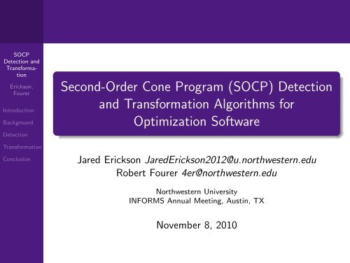
<strong>SOCP</strong><strong>Detection</strong> <strong>and</strong>TransformationErickson,FourerIntroductionBackground<strong>Detection</strong>TransformationConclusion<strong>Second</strong>-<strong>Order</strong> <strong>Cone</strong> <strong>Program</strong> (<strong>SOCP</strong>) <strong>Detection</strong><strong>and</strong> Transformation Algorithms forOptimization SoftwareJared Erickson JaredErickson2012@u.northwestern.eduRobert Fourer 4er@northwestern.eduNorthwestern UniversityINFORMS Annual Meeting, Austin, TXNovember 8, 2010
<strong>SOCP</strong><strong>Detection</strong> <strong>and</strong>TransformationErickson,FourerIntroductionBackground<strong>Detection</strong>TransformationConclusion1 Introduction2 Background3 <strong>Detection</strong>4 Transformation5 Conclusion
<strong>Second</strong>-<strong>Order</strong> <strong>Cone</strong> <strong>Program</strong>s (<strong>SOCP</strong>s)<strong>SOCP</strong><strong>Detection</strong> <strong>and</strong>TransformationErickson,FourerIntroductionBackground<strong>Detection</strong>TransformationConclusionCan be written as a quadratic programNot positive semi-definiteConvexEfficiently solvable with interior-point methods<strong>SOCP</strong> general form:minimize f T xsubject to ‖A i x + b i ‖ 2 ≤ (c T ix + d i ) 2 ∀ ic T ix + d i ≥ 0 ∀ i
Introduction<strong>SOCP</strong><strong>Detection</strong> <strong>and</strong>TransformationErickson,FourerIntroductionBackground<strong>Detection</strong>TransformationConclusionPrevious situation:<strong>SOCP</strong>s can be written in numerous equivalent formsThe form a modeler wants to use may not be the form asolver acceptsConverting the problem for a particular interior-pointsolver is tedious <strong>and</strong> error-proneIdeal situation:Write in modeler’s form in a general modeling languageAutomatically transform to a st<strong>and</strong>ard quadraticformulationTransform as necessary for each <strong>SOCP</strong> solver
Motivating Example<strong>SOCP</strong><strong>Detection</strong> <strong>and</strong>TransformationErickson,FourerIntroductionBackground<strong>Detection</strong>TransformationConclusionOriginal:minimizeTransformed:√√(x + 2) 2 + (y + 1) 2 + (x + y) 2minimize u + v(x + 2) 2 + (y + 1) 2 ≤ u 2(x + y) 2 ≤ v 2u, v ≥ 0
Motivating Example<strong>SOCP</strong><strong>Detection</strong> <strong>and</strong>TransformationErickson,FourerIntroductionBackground<strong>Detection</strong>TransformationConclusion<strong>Ampl</strong> model:var x; var y;var u >= 0; var v >= 0;minimize obj: u+v;s.t. C1: (x+2)^2+(y+1)^2
Motivating Example<strong>SOCP</strong><strong>Detection</strong> <strong>and</strong>TransformationErickson,FourerOriginal:minimize√√(x + 2) 2 + (y + 1) 2 + (x + y) 2IntroductionBackground<strong>Detection</strong>TransformationConclusionTransformed:minimize u + vr 2 + s 2 ≤ u 2t 2 ≤ v 2x + 2 = ry + 1 = sx + y = tu, v ≥ 0
TypologieL’habitat individuelArchitecturesa n c i e n n e sLES FORMES GROUPEESDestinées à l’origine à une population de classe moyenne ou modeste, les maisons groupées sont conçues dans unesprit d’économie. Alignées sur la rue ou en retrait derrière un jardinet, elles sont d’un gabarit réduit. Elles peuventêtre quasiment contemporaines à certaines maisons de bourg, mais s’en distinguent par le style d’architecture,refletant l’industrialisation, qui emploie les techniques modernes de la fin du XIXe siècle : la brique, l’enduit au ciment/chauxhydraulique. Ces maisons peuvent présenter différents modes d’implantation et types de modénatures.On distingue parmi ces maisons de ville populaires le type spécifique de la maison ouvrière Cacheux, et des petitsalignements de pavillons fin XIXe.La maison CacheuxLes maisons datent des années 1870. Témoignages trèsimportants des prémices de l’histoire du logement social,ces maisons sont des vestiges de l’oeuvre d’Emile Cacheux,pionnier du logement social en France.Elles sont groupées par deux ou par quatre, implantées àl’alignement sur rue ou en retrait avec clôture à l’alignement.Gabarit : généralement R+1 ; 2 travéesFaçade : Composition : régulièreMatériaux : maçonnerie de moellons enduite deciment et chaux hydrauliquePercements : baies régulières aux allèges bassesModénatures, décor : Modénatures simplesExceptionnellement, décor plâtre mouluré (ex.photo)Menuiseries : fenêtres bois peint à l’origineportes d’entrée soignées, souvent en bois, avec desjours en fer et verre, et des encadrements moulurés.Ferronneries : simples généralement en fontemoulée ou garde-corps ouvragés.ToitureVolumétrie : toit à deux pans, faîtage parallèle à larueMatériaux : tuile mécaniquePavillons alignés fin XIXeOn retrouve d’autres alignements dans le lotissement de Chassagnole. Leur caractéristique est de posséderdes façades élégantes revêtues d’enduit de plâtre et dotées d’un décor de plâtre mouluré reprenant les canonsde l’architecture classique : pilastres plats, linteaux à entablements… Elles sont implantées entre cour sur rueet jardin à l’arrière.PLU de la commune des Lilas - 6c6 - Cahier de recomm<strong>and</strong>ations architecturales - PLU approuvé le 14 Novembre 2007 - EspaceVille 9
Generally Accepted <strong>SOCP</strong> Form<strong>SOCP</strong><strong>Detection</strong> <strong>and</strong>Transformation<strong>SOCP</strong> general form:Erickson,FourerIntroductionBackground<strong>Detection</strong>TransformationConclusionminimize f T xsubject to ‖A i x + b i ‖ ≤ ciTwherex ∈ R n is the variablef ∈ R nA i ∈ R m i ,nb i ∈ R m ic i ∈ R nd i ∈ Rx + d i ∀i
St<strong>and</strong>ard Quadratic Form<strong>SOCP</strong><strong>Detection</strong> <strong>and</strong>TransformationErickson,FourerIntroductionBackground<strong>Detection</strong>TransformationConclusionObjective: a 1 x 1 + · · · + a n x nConstraints:Quadratic <strong>Cone</strong>: b 1 x 2 1 + · · · + b nx 2 n − b 0 x 2 0 ≤ 0where b i ≥ 0 ∀ i, x 0 ≥ 0Rotated Quadratic <strong>Cone</strong>: c 2 x 2 2 + · · · + c nx 2 n − c 1 x 0 x 1 ≤ 0where c i ≥ 0 ∀ i, x 0 ≥ 0, x 1 ≥ 0Linear Inequality: d 0 + d 1 x 1 + · · · + d n x n ≤ 0Linear Equality: e 0 + e 1 x 1 + · · · + e n x n = 0Variable: k L ≤ x
First Case: Sum <strong>and</strong> Max of Norms<strong>SOCP</strong><strong>Detection</strong> <strong>and</strong>TransformationErickson,FourerIntroductionBackground<strong>Detection</strong>TransformationConclusionAny combination ofsum,max, <strong>and</strong>constant multipleof norms can be represented as a <strong>SOCP</strong>.
Sum of Norms<strong>SOCP</strong><strong>Detection</strong> <strong>and</strong>TransformationErickson,FourerIntroductionBackground<strong>Detection</strong>TransformationConclusion=⇒minimizesubject tominimizep∑i=1q i∑j=1y iu 2 ij − y 2ip∑‖F i x + g i ‖i=1≤ 0, i = 1..p(F i x + g i ) j − u ij = 0, i = 1..p, j = 1..q iy i ≥ 0, i = 1..p
Max of Norms<strong>SOCP</strong><strong>Detection</strong> <strong>and</strong>TransformationErickson,FourerIntroductionBackground<strong>Detection</strong>TransformationConclusion=⇒minimize ysubject tominimize maxi=1..p ‖F ix + g i ‖q i∑uij 2 − y 2 ≤ 0, i = 1..pj=1(F i x + g i ) j − u ij = 0, i = 1..p, j = 1..q iy i ≥ 0, i = 1..p
Combination<strong>SOCP</strong><strong>Detection</strong> <strong>and</strong>TransformationErickson,FourerIntroductionBackground<strong>Detection</strong>TransformationConclusion=⇒minimize 4 max{3‖F 1 x + g 1 ‖ + 2‖F 2 x + g 2 ‖, 7‖F 3 x + g 3 ‖}minimize 4ysubject to 3u 1 + 2u 2 − y ≤ 07u 3 − y ≤ 0q i∑j=1v 2ij − u 2 i ≤ 0, i = 1, 2, 3(F i x + g i ) j − v ij = 0, i = 1, 2, 3, j = 1..q iu i ≥ 0, i = 1, 2, 3
Expression Tree Example<strong>SOCP</strong><strong>Detection</strong> <strong>and</strong>TransformationErickson,FourerIntroduction√√(x + 2) 2 + (y + 1) 2 + (x + y) 2+Background<strong>Detection</strong>TransformationConclusionsqrt+sqrt^2^2^2+++xyx2y1
Sum <strong>and</strong> Max of Norms (SMN) <strong>Detection</strong> Function<strong>SOCP</strong><strong>Detection</strong> <strong>and</strong>TransformationErickson,FourerIntroductionBackground<strong>Detection</strong>TransformationConclusion<strong>Detection</strong> Rules for SMN:Constant: f (x) = c is SMN.Variable: f (x) = x i is SMN.Sum: f (x) = ∑ ni=1 f i(x) is SMN if all the children f i are SMN.Product: f (x) = cg(x) is SMN if c is a positive constant <strong>and</strong>g is SMN.Maximum: f (x) = max{f 1 (x), . . . , f n (x)} is SMN if all thechildren f i are SMN.Square Root: f (x) = √ g(x) is SMN if g is NS.
Norm Squared (NS) <strong>Detection</strong> Function<strong>SOCP</strong><strong>Detection</strong> <strong>and</strong>TransformationErickson,FourerIntroductionBackground<strong>Detection</strong>TransformationConclusion<strong>Detection</strong> Rules for NS:Constant: f (x) = c is NS if c ≥ 0.Sum: f (x) = ∑ ni=1 f i(x) is NS if all the children f i are NS.Product: f (x) = cg(x) is NS if c is a positive constant <strong>and</strong> gis NS.Squared: f (x) = g(x) 2 is NS if g is linear.Maximum: f (x) = max{f 1 (x), . . . , f n (x)} is NS if all thechildren f i are NS.
<strong>Detection</strong> Example<strong>SOCP</strong><strong>Detection</strong> <strong>and</strong>TransformationErickson,FourerSum: f (x) = ∑ ni=1 f i(x) is SMN if all the children f i are SMN.+IntroductionBackgroundsqrtsqrt<strong>Detection</strong>Transformation+^2Conclusion^2^2+++xyx2y1
<strong>Detection</strong> Example<strong>SOCP</strong><strong>Detection</strong> <strong>and</strong>TransformationErickson,FourerSquare Root: f (x) = √ g(x) is SMN if g(x) is NS.+IntroductionBackgroundsqrtsqrt<strong>Detection</strong>Transformation+^2Conclusion^2^2+++xyx2y1
<strong>Detection</strong> Example<strong>SOCP</strong><strong>Detection</strong> <strong>and</strong>TransformationErickson,FourerSum: f (x) = ∑ ni=1 f i(x) is NS if all the children f i are NS.+IntroductionBackgroundsqrtsqrt<strong>Detection</strong>Transformation+^2Conclusion^2^2+++xyx2y1
<strong>Detection</strong> Example<strong>SOCP</strong><strong>Detection</strong> <strong>and</strong>TransformationErickson,FourerSquared: f (x) = g(x) 2 is NS if g is linear.+IntroductionBackgroundsqrtsqrt<strong>Detection</strong>Transformation+^2Conclusion^2^2+++xyx2y1
Transformation Process<strong>SOCP</strong><strong>Detection</strong> <strong>and</strong>TransformationErickson,FourerIntroductionBackground<strong>Detection</strong>TransformationConclusion1) Determine objective or constraint type with detection rules2) Apply corresponding transformation algorithmSeparate algorithm, starts at rootUses no information from detectionCreates new variables <strong>and</strong> constraintsNew constraints are formed by adding terms to functions
Transformation Conventions<strong>SOCP</strong><strong>Detection</strong> <strong>and</strong>TransformationErickson,FourerIntroductionBackground<strong>Detection</strong>TransformationConclusionx: vector of variables in the original formulationv: vector of variables in the original formulation <strong>and</strong> variablescreated during transformationf (x), g(x), h(x): functions from the original formulationFunctions created during transformation:o(v): objectives (linear)l(v): linear inequalitiese(v): linear equalitiesq(v): quadratic conesr(v): rotated quadratic conesc(v): expressions that could fit in multiple categories
Constraint Building Example<strong>SOCP</strong><strong>Detection</strong> <strong>and</strong>TransformationErickson,FourerIntroductionBackground<strong>Detection</strong>TransformationConclusionStep 1: l 1 (v) := 3x 1 + 2Step 2: l 1 (v) := l 1 (v) + v 3Step 3: l 1 (v) ≤ 0Result: 3x 1 + 2 + v 3 ≤ 0
Transformation Functions<strong>SOCP</strong><strong>Detection</strong> <strong>and</strong>TransformationErickson,FourerIntroductionBackground<strong>Detection</strong>TransformationConclusionnewvar(b)n + +Introduce new variable v n to variable vector vif b is specifiedSet lower bound of v n to belseSet lower bound of v n to −∞newfunc(c)m c + +Introduce new objective or constraint function of type cc mc (v) := 0
transformSMN<strong>SOCP</strong><strong>Detection</strong> <strong>and</strong>TransformationErickson,FourerIntroductionBackground<strong>Detection</strong>TransformationConclusiontransformSMN(f (x), c(v), k)switchcase f (x) = g(x) + h(x)transformSMN(g(x), c(v), k)transformSMN(h(x), c(v), k)case f (x) = ∑ i f i(x)transformSMN(f i (x), c(v), k) ∀ icase f (x) = αg(x)transformSMN(g(x), c(v), kα)
transformSMN<strong>SOCP</strong><strong>Detection</strong> <strong>and</strong>TransformationErickson,FourerIntroductionBackground<strong>Detection</strong>TransformationConclusioncase f (x) = max i f i (x)newvar()c(v) := c(v) + kv nnewfunc(l): l ml (v) := −v nfor i ∈ ItransformSMN(f i (x), l ml (v), 1)case f (x) = √ g(x)newvar(0)c(v) := c(v) + kv nnewfunc(q): q mq (v) := −v 2 ntransformNS(g(x), q mq (v), 1)
transformNS<strong>SOCP</strong><strong>Detection</strong> <strong>and</strong>TransformationErickson,FourerIntroductionBackground<strong>Detection</strong>TransformationConclusiontransformNS(f (x), q(v), k)switchcase f (x) = g(x) + h(x)transformNS(g(x), c(v), k)transformNS(h(x), c(v), k)case f (x) = ∑ i f i(x)transformNS(f i (x), c(v), k) ∀ icase f (x) = αg(x)transformNS(g(x), c(v), kα)
transformNS<strong>SOCP</strong><strong>Detection</strong> <strong>and</strong>TransformationErickson,FourerIntroductionBackground<strong>Detection</strong>TransformationConclusioncase f (x) = g(x) 2newvar()q(v) := q(v) + kv 2 nnewfunc(e): e me (v) := g(x) − v ncase f (x) = max i f i (x)newvar()q(v) := q(v) + kv 2 nfor i ∈ Inewfunc(q): q mq (v) := −v 2 ntransformNS(f i (x), q mq (v), 1)
Transformation Example<strong>SOCP</strong><strong>Detection</strong> <strong>and</strong>TransformationErickson,FourerIntroductionBackground<strong>Detection</strong>TransformationConclusionf (x) =√√(x + 2) 2 + (y + 1) 2 + (x + y) 2f (x) is SMN ⇒ apply corresponding transformation algorithmSet all index variables to 0o(v) := 0transformSMN(f (x), o(v), 1)
Transformation Example<strong>SOCP</strong><strong>Detection</strong> <strong>and</strong>TransformationErickson,FourerIntroductionBackground<strong>Detection</strong>TransformationConclusionf (x) =case f (x) = √ g(x)newvar(0)o(v) := o(v) + v 1newfunc(q): q 1 (v) := −v 2 1transformNS(g(x), q 1 (v), 1)√(x + 2) 2 + (y + 1) 2+sqrt+sqrt^2^2^2+++xyx2y1
Transformation Example<strong>SOCP</strong><strong>Detection</strong> <strong>and</strong>TransformationErickson,FourerIntroductionBackgroundf (x) = (x + 2) 2 + (y + 1) 2case f (x) = g(x) + h(x)transformNS(g(x), q 1 (v), k)transformNS(h(x), q 1 (v), k)<strong>Detection</strong>TransformationConclusionsqrt+sqrt+^2^2^2+++xyx2y1
Transformation Example<strong>SOCP</strong><strong>Detection</strong> <strong>and</strong>TransformationErickson,FourerIntroductionBackground<strong>Detection</strong>TransformationConclusionf (x) = (x + 2) 2case f (x) = g(x) 2newvar()q 1 (v) := q 1 (v) + v 2 2newfunc(e): e 1 (v) := g(x) − v 2+sqrt+sqrt^2^2^2+++xyx2y1
Current Functions<strong>SOCP</strong><strong>Detection</strong> <strong>and</strong>TransformationErickson,FourerIntroductionBackground<strong>Detection</strong>TransformationConclusiono(v) = v 1q 1 (v) = v2 2 − v12e 1 (v) = x + 2 − v 2v 1 ≥ 0
Final Functions<strong>SOCP</strong><strong>Detection</strong> <strong>and</strong>TransformationErickson,FourerIntroductionBackground<strong>Detection</strong>TransformationConclusiono(v) = v 1 + v 4q 1 (v) = v2 2 + v3 2 − v1 2 ≤ 0e 1 (v) = x + 2 − v 2 = 0e 2 (v) = y + 1 − v 3 = 0q 2 (v) = v5 2 − v4 2 ≤ 0e 3 (v) = x + y − v 5 = 0v 1 ≥ 0v 4 ≥ 0
Motivating Example<strong>SOCP</strong><strong>Detection</strong> <strong>and</strong>TransformationErickson,FourerOriginal:minimize√√(x + 2) 2 + (y + 1) 2 + (x + y) 2IntroductionBackground<strong>Detection</strong>TransformationConclusionTransformed:minimize u + vr 2 + s 2 ≤ u 2t 2 ≤ v 2x + 2 = ry + 1 = sx + y = tu, v ≥ 0
Other Objective Forms<strong>SOCP</strong><strong>Detection</strong> <strong>and</strong>TransformationErickson,FourerIntroductionBackground<strong>Detection</strong>TransformationConclusionNorm Squared:Fractional:minimizeminimizewhere a i x + b i > 0 ∀ iLogarithmic Chebyshev:p∑c i (a i x + b i ) 2i=1p∑i=1c i ‖F i x + g i ‖ 2a i x + b iwhere a i x > 0minimize maxi=1..p | log(a ix) − log(b i )|
Other Objective Forms<strong>SOCP</strong><strong>Detection</strong> <strong>and</strong>TransformationErickson,FourerIntroductionBackground<strong>Detection</strong>TransformationConclusionProduct of Positive Powers:p∏maximize (a i x + b i ) α ii=1where α i > 0, α i ∈ Q, a i x + b i ≥ 0Product of Negative Powers:p∏minimize (a i x + b i ) −π ii=1where π i > 0, π i ∈ Q, a i x + b i ≥ 0Combinations of these forms made by sum, max, <strong>and</strong>positive constant multiple, except Log Chebyshev <strong>and</strong>some cases of Product of Positive Powers. Example:minimize max{p∑(a i x+b i ) 2 ,i=1q∑j=1‖F j x + g j ‖ 2y j}+r∏(c k x) −π kk=1
Constraint Forms<strong>SOCP</strong><strong>Detection</strong> <strong>and</strong>TransformationErickson,FourerIntroductionBackground<strong>Detection</strong>TransformationConclusionSum <strong>and</strong> Max of Norms:p∑c i ‖F i x + g i ‖ ≤ ax + bi=1Norm Squared:p∑c i (a i x + b i ) 2 ≤ c 0 (a 0 x + b 0 ) 2i=1where c 0 ≥ 0, a 0 x + b 0 ≥ 0Fractional:p∑i=1where a i x + b i > 0 ∀ ik i ‖F i x + g i ‖ 2a i x + b i≤ cx + d
Constraint Forms<strong>SOCP</strong><strong>Detection</strong> <strong>and</strong>TransformationErickson,FourerIntroductionBackground<strong>Detection</strong>TransformationConclusionProduct of Positive Powers:∑− ∏ (a ji x + b ji ) π ji≤ cx + dj iwhere a ji x + b ji ≥ 0, π ji > 0, ∑ i π ji ≤ 1∀jProduct of Negative Powers:∑ ∏(a ji x + b ji ) −π ji≤ cx + dj iwhere a ji x + b ji ≥ 0, π ji > 0Combinations of these forms made by sum, max, <strong>and</strong>positive constant multiple
Conclusion<strong>SOCP</strong><strong>Detection</strong> <strong>and</strong>TransformationErickson,FourerIntroductionBackground<strong>Detection</strong>TransformationConclusionImplementation for AMPL <strong>and</strong> several solversPaper documenting algorithmsExtend to functions not included in AMPL
References<strong>SOCP</strong><strong>Detection</strong> <strong>and</strong>TransformationErickson,FourerAlizadeh, F. <strong>and</strong> D. Goldfarb. <strong>Second</strong>-order cone programming.Math. <strong>Program</strong>., Ser B 95:3–51, 2003.IntroductionBackground<strong>Detection</strong>TransformationConclusionLobo, M.S., V<strong>and</strong>enberghe, S. Boyd, <strong>and</strong> H. Lebret.Applications of second order cone programming. Linear AlgebraAppl. 284:193–228, 1998.Nesterov, Y. <strong>and</strong> A. Nemirovski. Interior Point PolynomialMethods in Convex <strong>Program</strong>ming: Theory <strong>and</strong> Applications.Society for Industrial <strong>and</strong> Applied Mathematics (SIAM),Philadelphia, 1994.
Thank You<strong>SOCP</strong><strong>Detection</strong> <strong>and</strong>TransformationErickson,FourerIntroductionBackground<strong>Detection</strong>TransformationConclusionJaredErickson2012@u.northwestern.eduThis work was supported in part by grant CMMI-0800662 fromthe National Science Foundation.