Harris Corner Detector - Multimedia Computing and Computer ...

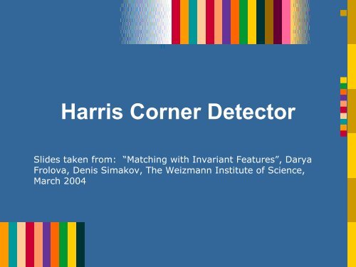
Harris Corner DetectorSlides taken from: “Matching with Invariant Features”, DaryaFrolova, Denis Simakov, The Weizmann Institute of Science,March 2004

An introductory example:C.Harris, M.Stephens. “A Combined Corner and Edge Detector”. 1988

The Basic Idea• We should easily recognize the point bylooking through a small window• Shifting a window in any direction shouldgive a large change in intensity

Basic Idea (2)“flat” region:no change inall directions“edge”:no change alongthe edge direction“corner”:significant changein all directions

MathematicsChange of intensity for the shift [u,v]:E u ,v=∑x , yHarris Detector:Mathematicsw x , y[I xu , yv−I x , y] 2WindowfunctionShiftedintensityIntensityWindow function w(x,y) =or1 in window, 0 outsideGaussian

MathematicsFor small shifts [u,v] we have a bilinear approximation:E u ,v≃[u v ]M[ u v]where M is a 2×2 matrix computed from image derivatives:M =∑x , yw x , y[ I 2xI xI y]2I xI yI y

(λ max) -1/2 (λ min) -1/2MathematicsIntensity change in shifting window: eigenvalue analysisM =∑x , yw x , y[ I 2xI xI y]2I xI yI yλ 1, λ 2– eigenvalues of MEllipse E(u,v) = constdirection of thefastest changedirection of theslowest change

MathematicsClassification ofimage points usingeigenvalues of M:λ 2“Edge”λ 2>> λ 1“Corner”λ 1and λ 2are large,λ 1~ λ 2;E increases in alldirectionsλ 1and λ 2are small;E is almost constantin all directions“Flat”region“Edge”λ 1>> λ 2λ 1

MathematicsMeasure of corner response:R=det M −k trace M 2det M = 1 2trace M = 1 2(k – empirical constant, k = 0.04-0.06)

Mathematics• R depends only oneigenvalues of Mλ 2“Edge”R < 0“Corner”• R is large for a corner• R is negative with largemagnitude for an edgeR > 0• |R| is small for a flatregion“Flat”|R| small“Edge”R < 0λ 1

Harris Detector• The Algorithm:– Find points with large corner responsefunction R (R > threshold)– Take the points of local maxima of R

Harris Detector: Workflow

Harris Detector: WorkflowCompute corner response R

Harris Detector: WorkflowFind points with large corner response: R>threshold

Harris Detector: Workflow

Harris Detector: Summary• Average intensity change in direction [u,v] can beexpressed as a bilinear form:E u ,v≃[u v ]M[ u v]• Describe a point in terms of eigenvalues of M:measure of corner responseR=det M −k trace M 2• A good (corner) point should have a large intensitychange in all directions, i.e. R should be largepositive

Harris Detector: Properties• Rotation invariance• Ellipse rotates but its shape (i.e. eigenvalues)remains the same

Harris Detector: Properties• Partial invariance to affine intensity change• Only derivatives are used => invariance tointensity shift I → I + b• Intensity scale: I → a I

Harris Detector: Properties• But: non-invariant to image scale!edgecorner

Face RecognitionSlides taken from Jeremy Wyatt(“www.cs.bham.ac.uk/~jlw/vision/face_recognition.ppt”)

Eigenfaces: The Idea• Think of a face as being a weighted combination of some“component” or “basis” faces• These basis faces are called eigenfaces…-8029 2900 1751 1445 4238 6193

Face Representation• These basis faces can be differently weighted to represent any face• So we can use different vectors of weights to represent differentfaces-8029 -1183 2900 -2088 1751 -4336 1445 -669 4238 -4221 6193 10549

Learning Eigenfaces• How do we pick the set of basis faces?• We take a set of real training faces…Then we find (learn) a set of basis faces which best represent thedifferences between themWe’ll use a statistical criterion for measuring this notion of “bestrepresentation of the differences between the training faces”We can then store each face as a set of weights for those basis faces

Using Eigenfaces: Recognition &Reconstruction• We can use the eigenfaces in two ways• 1: we can store and then reconstruct a face from a set of weights• 2: we can recognize a new picture of a familiar face

Learning Eigenfaces• How do we learn them?• We use a method called Principal ComponentAnalysis (PCA)• To understand it we will need to understand– What an eigenvector is– What covariance is• But first we will look at what is happening in PCAqualitatively

Subspaces• Imagine that our face is simply a (high dimensional) vector of pixels• We can think more easily about 2D vectors• Here we have data in two dimensions• But we only really need one dimension to represent it

Finding Subspaces• Suppose we take a line through the space• And then take the projection of each point onto that line• This could represent our data in “one” dimension

Finding Subspaces• Some lines will represent the data in this way well, some badly• This is because the projection onto some lines separates the datawell, and the projection onto some lines separates it badly

Finding Subspaces• Rather than a line we can perform roughly the same trick with avectorΦ =16ν32 νν⎡1⎤= ⎢1 ⎥⎣ ⎦• Now we have to scale the vector to obtain any point on the lineΦ =iµ ν

EigenvectorsAn eigenvector is a vectorvthat obeys the following rule:AAv= µ vWhere is a matrix, and µ is a scalar (called the eigenvalue)• Only square matrices have eigenvectors• Not all square matrices have eigenvectors• An n by n matrix has at most n distinct eigenvectors• All the distinct eigenvectors of a matrix are orthogonal

Covariance• Which single vector can be used to separate these points as much aspossible?x 2• This vector turns out to be a vector expressing the direction of thecorrelation• Here are two variables x1and x2• They co-vary (y tends to change in roughly the same direction as x)x 1

Covariance• The covariances can be expressed as a matrixx 1x 2.617 .615C = ⎡ ⎤⎢.615 .717 ⎥⎣⎦x 1x 2x 2• The diagonal elements are the variances e.g. Var(x 1)• The covariance of two variables is:cov( x , x ) =1 2n∑i = 1( x − x )( x − x )ii1 1 2 2n − 1x 1

Eigenvectors of the covariancematrix• The covariance matrix has eigenvectorscovariance matrixeigenvectorseigenvaluesν1.617 .615C = ⎡ ⎤⎢.615 .717 ⎥⎣⎦⎡ − .735⎤= ⎢.678 ⎥⎣ ⎦ν2⎡ .678⎤= ⎢.735 ⎥⎣ ⎦µ1= 0.049µ2= 1.284x 2x 1• Eigenvectors with larger eigenvaluescorrespond to directions in which thedata varies more• Finding the eigenvectors and eigenvalues ofthe covariance matrix for a set of data is calledprincipal component analysis

Expressing points• Suppose you think of your eigenvectors as specifying a new vectorspace• i.e. one can reference any point in terms of those eigenvectors• A point’s position in this new coordinate system is what we earlierreferred to as its “weight vector”• For many data sets you can cope with fewer dimensions in the newspace than in the old space

Eigenfaces• In the face case:– the face is a point in a high-dimensional space– the training set of face pictures is our set of points• Training:– calculate the covariance matrix of the faces– find the eigenvectors of the covariance matrix• These eigenvectors are the eigenfaces or basis faces• Eigenfaces with bigger eigenvalues will explain moreof the variation in the set of faces, i.e. will be moredistinguishing

Eigenfaces: image space to facespace• When we see an image of a face we can transform it to facespaceiwk=• There are k=1…n eigenfacesi• The i th face in image space is a vector x• The corresponding weight is w k• We calculate the corresponding weight for every eigenfacex.vv kk

Recognition in face space• Recognition is now simple. We find the euclidean distance dbetween our face and all the other stored faces in face space:( ) 2i in1 2 1 2d( w , w ) = w − w• The closest face in face space is the chosen match∑i = 1

Reconstruction• The more eigenfaces you have the better the reconstruction, but youcan have high quality reconstruction even with a small number ofeigenfaces82 70 5030 20 10

Summary• Statistical approach to visual recognition• Also used for object recognition• Problems• Reference: M. Turk and A. Pentland (1991). Eigenfacesfor recognition, Journal of Cognitive Neuroscience, 3(1):71–86.