True Triaxial Piping Test Apparatus for Evaluation of Piping Potential ...

True Triaxial Piping Test Apparatus for Evaluation of Piping Potential inEarth StructuresKevin S. RichardsGraduate Research Assistant, Department of Civil and Materials Engineering, University ofIllinois at Chicago, 842 West Taylor Street, Chicago, Illinois 60607, USA,e-mail: kevinlaurie@sbcglobal.netKrishna R. ReddyProfessor, Department of Civil and Materials Engineering, University of Illinois at Chicago, 842West Taylor Street, Chicago, Illinois 60607, USA, e-mail: kreddy@uic.eduFinal Manuscript Submitted to:Geotechnical Testing Journal, ASTM1

True Triaxial Apparatus Piping Test Apparatus for Evaluation ofPiping Potential in Earthen StructuresABSTRACT: Current methods available for testing the piping potential of soils in dams (pinholetest, hole erosion test, slot erosion test) are limited to cohesive soils that maintain an openhole within the sample. These tests do not adequately simulate conditions within a zonedembankment, where zones of noncohesive materials are present under relatively high confiningstresses. A new apparatus, called true triaxial piping test apparatus or TTPTA, was developedfor testing a wider variety of soils under a wider range of confining stresses, hydraulic gradients,and pore pressures than current tests allow. The TTPTA is capable of applying a range ofconfining stresses along three mutually perpendicular axes in a true-triaxial test apparatus. Porepressures are also controlled through regulated inlet and outlet pressures. The test determines thecritical hydraulic gradient and, more importantly, the critical hydraulic velocity at which pipingis initiated in non-cohesive soils. Detailed descriptions of the test apparatus and test method arepresented, as are initial test results using TTPTA. Three sets of initial tests were conducted usinguniform sand to (1) assess the repeatability of test results, (2) evaluate how the rate of change ofin-flow impacts the critical dischare rate at which piping is initiated, and (3) evaluate how theangle of seepage affects the critical velocity for piping initiation These initial tests wereconducted to evaluate the method and to help set test parameters for future testing. It is foundthat the TTPTA is capable of yielding fairly consistent results with 10% scatter in repeat tests.The seepage angle tests demonstrate that the angle between seepage flow direction and thedirection of gravity is an important factor to consider when evaluating piping potential. The rateof change in seepage also has a minor influence on test results, but a change in flow rate of 52

(ml/min)/min could produce reliable results. Based on the results, the hydraulic gradient is foundto be a less reliable indicator of piping potential than the hydraulic velocity for noncohesivesoils. The TTPTA is capable of simulating conditions within small to medium sizedembankments.KEYWORDS: piping potential, piping tests, critical hydraulic gradient, critical hydraulicvelocity, true triaxial piping testINTRODUCTIONNumerous earth structures, particularly earth dams, commonly fail by piping. In fact,approximately half of all dam failures are due to piping (Foster, Fell, and Spangle, 2000), withapproximately 33% of all piping failures possibly attributed to backwards erosion piping(Richards and Reddy, 2007). Different modes of piping failure have been recognized in theliterature and are defined by the mechanism causing the piping. The modes commonlyrecognized include backwards erosion, internal erosion, tunneling, suffusion, and heave(Richards and Reddy, 2007). In order to evaluate piping potential in earthen dams, the firststandardized laboratory piping tests were developed in the 1970’s; commonly known as thepinhole test, ASTM D4647-93, and the double hydrometer test, ASTM D4221-99 (Sherard et al.,1976, Decker and Dunnigan, 1977). The tests were originally developed to assess pipingpotential due to the dispersivity of soils. Dispersive soils are highly prone to piping failure(Aitchison, et al., 1963) and these tests were specifically developed to evaluate a soil’s pipingpotential in areas with dispersive soils. Prior to these early laboratory tests, empirical methodswere available to assess piping potential. Bligh (1910) recommended percolation factors for3

various types of non-cohesive soils based on empirical data. Bligh’s method was later improvedby the work of Lane (1934). These empirical methods have a significant shortcoming; they arebased on seepage flow paths consistent with internal erosion and do not adequately address thepotential for backwards erosion. Terzaghi (1922) developed the classic theory of heave, which isbased on theoretical application of soil mechanics. This theory is commonly used to evaluatepiping potential. However, Terzaghi’s theory does not consider the physico-chemical or otherproperties of soils that influence piping potential. It was originally based on the case whereseepage flow is vertically upward into a cofferdam, acting in direct opposition to the downwardforce of gravity. Does this theory apply equally to the case with seepage exiting at a downwardangle on the downstream slope of an embankment dam? No standardized laboratory tests havebeen developed to assess piping potential in non-cohesive soils that could be used to evaluatepiping potential in a way that would take all these other factors into account.Some new tests were recently developed to study erosion potential of cracks in embankmentdams. The Hole Erosion Test (HET) and Slot Erosion Test (SET) were developed for thispurpose in 2004 (Wan and Fell, 2002, 2004). These tests are designed to assess the erosion rateindex of soils subjected to concentrated leaks, for research into the rate of erosion for breachanalyses and also have application in risk assessments. However, the HET and SET may not bedirectly applicable to cases of backwards erosion piping since the mode of piping beingevaluated in these tests is interior erosion. A number of other tests have been developed toassess surficial erosion, such as occurs in cases of overtopping failures of embankment dams oraround bridge abutments; however, these also are not directly applicable to backwards erosion4

piping. These include the jet erosion and rotating cylinder tests (Moore and Masch, 1962) andthe erosion function apparatus (EFA) (Briaud et al., 2001).This paper first provides a critical review of current piping test methods, and then describes thedevelopment of true triaxial piping test apparatus and the sample preparation and testing. Finally,a series of experimental results are presented to investigate reproducibility of the test results andthe effects of rate of in-flow and angle of seepage on piping initiation.CURRENT PIPING TEST METHODSThe pinhole test (ASTM D4647-93) was developed by Sherard et al. (1976) to assess thepresence of dispersive clay in soils, which is known to increase the risk of piping in embankmentdams (Aitchison et al., 1963). The test is not applicable to soils with less than 12% fraction finerthan 0.005 mm and with a plasticity index less than or equal to 4. The test consists of a tubesealed at both ends with steel or aluminum plates and o-rings. Gravel drains are placed at eitherend of the tube with a 1.5 inch long section of compacted soil sandwiched between the drains. Amanometer or other device controls the inlet pressure at one end of the cylinder; the other end isopen to atmospheric pressure. The test is conducted with the cylinder in the horizontal position.Water is allowed to flow through the sample for anywhere from 5 to 10 minutes under each headcondition. To facilitate the erosion process, a 1.0 mm pinhole is punched through the center ofthe compacted soil. The test is conducted by gradually increasing the inlet pressure from 2-inch(50-mm), to 7-inch (180-mm), to 15-inch (380-mm), to 40-inch (1020-mm) head. The dischargerate is measured and visually inspected for clarity. The test is conducted until the clarity of thedischarge and flow rate indicate that piping has progressed. The soil is rated into one of five5

categories, based on the head at which the piping commenced, the amount of sediment in thedischarge (based on visual estimate of clarity) and the size of the eroded hole after the test.A recent advancement was the development of the HET and SET tests, developed by Wan andFell (2002). These tests were not specifically developed to assess soils for their backwardspiping characteristics. The HET and SET tests were designed to determine the erosion rate insoils subject to concentrated leaks, such as might occur in a crack through cohesive soils in thecore of a dam. The HET consists of compacting soil in a standard mold used for the compactiontest. A 6-mm hole is drilled through the sample and an increasing hydraulic head applied acrossthe sample with a constant 100 mm of water column applied at the outlet end of the sample. Thetest is done horizontally and is quite similar to the pinhole test, except for the dimensions of theapparatus and the hole diameter. The evaluation of the test is done differently than the pinholetest in that the hole diameter is computed from the flow rate rather than direct measurement. TheSET is similar to the HET with respect to evaluation of the data and computation of an erosionrate index, but the apparatus is a rectangular box 0.15 m wide, 0.1 m deep, and 1 m long. A slotis formed into the top of the soil, which is compacted into the box. In both the HET and SET,erosion occurs in a preformed pipe, similar to the pinhole test.Other tests, which may have application to suffusion and backwards erosion piping have beenreported in the literature. These tests were developed by a number of researchers (Valdes andLiang, 2006; Kakuturu, 2003; Tomlinson and Vaid, 2000; Skempton and Brogan, 1994; Bertram,1940) to evaluate various modes of piping behavior of soils. For example, Kakuturu, 2003developed tests and a method for prediction of the healing that occurs by self filtration.6

Skempton and Brogan, 1994 provided a method for evaluation of soils prone to suffusion (aprofound lack of self filtration). Valdes and Liang, 2006 and Bertram, 1940 evaluated theperformance of engineered filters. Tomlinson and Vaid, 2000 developed a test to evaluate theeffect of uniaxial stress on piping. Their test consisted of a uniaxially loaded sample of soilplaced in a vertical cylinder 10-cm in diameter and 10-cm long. There is a gravel drain(specifically designed to allow passage of sediments) at the bottom of the cylinder with a 1.5 mmmesh at the bottom. Soil piped through the coarse filter is allowed to collect in a pan at the baseof the apparatus. The soil is placed on top of the gravel drain with a 1.5 mm mesh at the top ofthe soil. Fluid is introduced in the top of the cylinder through holes drilled into a platen thatapplies a vertical load to the sample. The hydraulic head on the outlet side of the apparatus iscontrolled by submerging it in a large water bath with constant water level maintained.Hydraulic head to the inlet side is controlled by throttling a valve open to the water supplysystem line pressure. The maximum differential head achieved with this system is 100 cm ofwater. Flow rate was monitored by measuring the flow out of the water bath. The amount ofsediment in the fluid discharge is used to assess migration (piping) of particles. This test isunique in that it tests piping in a vertically oriented downward direction. They found that theconfining pressure, and the magnitude and rate of gradient increase may influence initiation ofpiping. Skempton and Brogan (1994) used a similar device but with flow being orientedvertically upward, to test piping potential in gap-graded soils. They were also interested incomparison of similar tests of internally unstable soils conducted on horizontally orientedsamples (Adel et al., 1988). These tests were used to assess the internal stability of gap gradedsoils.7

The pinhole test is a difficult test to run and is prone to premature clogging or self-healing of thepinhole. It works best in soils that can maintain an open pinhole under conditions of flow;hence, it works best in soils with cohesion and little self healing properties. The test is good fordiscerning dispersive from non-dispersive soils that meet these requirements, but it does notyield an erosion index or other parameters that might be useful for comparison between nondispersivesoils of wider gradations. The test is only applicable to internal erosion, erosion alongconcentrated leaks through pre-existing openings, and does not provide evaluation of backwardserosion piping potential. The hole and slot erosion tests are designed to yield specific erosionparameters, such as the erosion rate index, that can be used to assess the erodibility and rate oferosion of non-dispersive soils subjected to concentrated leaks through pre-existing openings.However, the hole erosion test is limited to cohesive soils that maintain an open hole under flowconditions. Since the diameter of the hole is greater than in the pinhole test, it is less prone toself healing or clogging. The slot erosion test can be used for soils with a wider range ofcohesion, but due to the proximity of the slot against the top of the cell, may be more indicativeof internal erosion potential (erosion along a soil-structure contact).Other tests discussed in the literature have similar limitations with respect to backwards erosionpotential in non-cohesive soils. For example, some are limited to testing suffusion or heave(Skempton and Brogan, 1994), and others are limited to testing internal erosion (Adel et al.,1988). Tomlinson and Vaid, 2000, presented a test that may have some application to backwardserosion potential. However, the geometry of the apparatus is limited to vertically downwardflow and therefore does not provide an adequate analog to backwards erosion piping in dams.8

In light of the drawbacks with current methods for testing piping in non-cohesive soils, a newinstrument was developed that could test a wider range of soils. The new instrument allows fortesting piping characteristics of soils within a range of hydraulic conditions and confiningstresses. An important difference between this new test and currently available tests is that thenew test is specifically designed to evaluate backwards erosion piping potential rather thanerosion along a pre-existing opening (internal erosion).TRUE TRIAXIAL PIPING TEST APPARATUS (TTPTA)General System Description and DiagramThe TTPTA was developed to permit testing a wider range of soil types, particularly noncohesivesoils, for backwards-erosion piping potential under variable confining pressureconditions. The TTPTA was perfected after two earlier prototypes were tested andimprovements made to the overall design and instrumentation. The apparatus is capable ofsimulating conditions within a small to medium sized zoned embankment dam. The apparatusprovids the critical hydraulic gradient and the critical hydraulic velocity required to initiatepiping, while recording such variables as the inlet flow rate, inlet and outlet pressure heads, massof discharged effluent per second, and differential pressure every 100 milliseconds. Theapparatus is constructed around a true-triaxial load cell capable of initiating backwards erosiontype piping under variable pore and confining pressures. The complete apparatus consists of anInlet-Outlet Pressure Control Panel, an Inlet-flow Control Panel, the True Triaxial Load Cell, anOutlet Tube, Inlet/Outlet Valve Trees, a Flow-Through Turbidimeter, and Pressurized WaterSource and Pressurized Receiving Vessels, and the Instrumentation and Data Logging9

Equipment. A photograph of the True Triaxial test cell, which is the heart of the system, isshown in Figure 1 and a diagram of the overall system is shown in Figure 2.Inlet-Outlet Pressure Control PanelThe purpose of the Inlet-Outlet Pressure Control Panel is to provide finely regulated air pressuresto the Pressurized Water Source, and Receiving Vessels. The panel is connected to a standard aircompressor/storage tank capable of supplying 100 psi (689 kPa) compressed air. The airpressure supplied through the control panel to the source and receiving vessels is regulated withair regulators capable of supplying constant air pressure from 0 to 15 psi (0 to 103 kPa). It alsois used to create and supply a vacuum to the True Triaxial Load Cell prior to saturating a loadedsample. The vacuum is also used to evacuate the Pressurized Water Source Vessel the nightbefore tests are run. This is done to ensure air is removed from the source water before runningthe test. The Inlet-Outlet Pressure Control Panel vacuum generator is capable of creating a -8.7psi (-60 kPa) vacuum. A water trap and a 0-90 psi (0-620 kPa) pressure regulator that suppliesair pressure to the Air Bladder Control Panel are also included on the panel, as are the varioustubing and quick release connectors required to connect all the equipment. A diagram of theInlet-Outlet Pressure Control Panel is shown in Figure 3, and a photograph of the Inlet-OutletPressure Control Panel in Figure 4a.Inlet-flow Control PanelThe Inlet-flow Control Panel (Figure 4b and Figure 5) conveys water from the Pressurized WaterSource Vessel to the True-Triaxial Load Cell through either a high-volume flow gage, or a lowvolumeflow gage, depending on what the sample requires. There is also a granular filter to10

further remove any entrained air (Bertram, 1940). A water filter is also used to remove anysediment or other impurities in the water. The inlet-flow control panel is also equipped withthree-way valves for switching between the high and low flow gages, and for switching to gageor bypass mode. The bypass mode allows tapping into the Pressurized Water Source whendeaired water is needed during the soil saturation procedure.True-Triaxial Load Cell SystemSeveral components make up the true-triaxial load cell system. There is the outer case, whichmakes up the load cell. Inside the load cell are three air bladder pistons, which provide theconfining stresses to the soil sample along three orthogonal directions. The stresses applied byeach of these air bladder pistons can be independently controlled; hence, it is a true-triaxial loadcell.Triaxial Load Cell ComponentsThe outer case of the Load Cell also serves as the reaction frame. It is composed of 1-inch (25mm) thick aluminum or Lexan plate. The outer case is held together with a flexible adhesive toseal the contacts (except along the bottom plate), and ¼ inch (6.3 mm) diameter stainless steelbolts. A rubber gasket is used along the bottom plate to allow its removal for loading the cell. A¼ inch (6.3 mm) hole is at one end of the top plate to provide an inlet for water, and a ½ inch(12.7 mm) hole is provided at the downstream end plate to provide an outlet. This outlet hole islocated near the bottom of the load cell and has a recessed flange for fitting a ½ inch (12.7 mm)diameter washer with an inside-hole sized for the outside diameter of the outlet pipe. Thewasher is attached to the pressure vessel with a flexible adhesive and when in-place should be11

flush with the inside face of the load cell. The outlet pipe should easily slide into the washerwith minimal space between the outside of the outlet pipe and inside of the washer. The end ofthe outlet pipe should fit flush with the inside face of the pressure vessel. Three sides of thepressure vessel have threaded ¼ inch (6.4 mm) holes to provide inlets for compressed air, whichfills the Air Bladder Pistons located inside the pressure vessel. The holes are fully penetratingand are threaded on both sides. These three holes are located along the primary axes of the soilsample and will provide the σ1, σ2, and σ3 stresses to the soil. The holes are offset to allowsome space for the bladders to inflate without interfering with each other. One of the bladders islocated at the top of the cell so that when inflated, it will help fill any voids between the cell walland soil due to minute settlement of the soil. The bottom piece also has a neoprene pad that alsohelps to prevent voids from forming by applying some pressure to the soil when the cover is puton after loading the sample. Finally, there are grooves cut on the inside walls of the left andright sides of the pressure vessel. The grooves allow a steel or aluminum plate to be temporarilyinserted prior to filling the vessel with gravel drain materials and the soil sample. The platesupports the gravel drain and screen prior to placing soil into the pressure vessel. Two other ¼inch (6.4 mm) diameter threaded holes are provided for monitoring the internal pore pressure atthe outlet and for monitoring differential pressure across the load cell.Air Bladder Control PanelFigure 4c shows the Air Bladder Control Panel. The air bladders are typically guaranteed to amaximum fill pressure that must not be exceeded during the test. This maximum pressure is thelimiting factor in the magnitude of loads and pore pressures that can be evaluated under this test.The compressed air that is supplied by the Inlet-Outlet Pressure Control Panel is conveyed to a12

manifold within the Air Bladder Control Panel. The manifold provides a three-way split of thesupplied air to three pressure regulators and equipped with glycerin-filled stainless steel gauges.The air bladders used in this research were guaranteed to a maximum 30-psi internal pressure;hence, the pressure regulators and gages in the Air Bladder Control Panel were designed for anoperating range of 0 to 30 psi (0 to 207 kPa), which is adequate for simulating internal stresseswithin small embankments or levees. The air regulators and gages could be changed if higherpressure air bladders are used in the Air Bladder Pistons for evaluations of conditions withinlarger embankments.Air Bladder PistonThe soil sample is subjected to stress by steel plates driven by air bladders. The steel plates andair bladders are enclosed in a flexible membrane to prevent seepage from bypassing the soilsample. The arrangement of a top and bottom steel plate sandwiching an air bladder, allenclosed in a latex cover, is what makes up an air bladder piston. A standard 4-inch (100 mm)triaxial membrane, 0.012 inches (0.3 mm) thick and 12 inches (305 mm) long will serve thispurpose. The piston components are assembled and inserted into the membrane sleeve. The twoends of the sleeve are glued and folded onto the bottom of the piston and attached to the insidewall of the Pressure Vessel with a flexible adhesive. The air bladders are equipped with maleNPT fittings for air inlet that screw into the load cell wall. Neoprene pads are also provided onthe steel plates that make contact with the soil to accommodate any small voids or bumps thatmay be present at the soil/piston surface and to help form a seal between the pistons and soil.The air bladders can be acquired from companies specializing in fabrication of custom airbladders, commonly used for lifting large heavy objects. There are a variety of materials that can13

e used to fabricate the air bladders depending on the amount of pressure that will be containedwithin the bladder. Higher pressure air bladders are generally more expensive. The dimensionsand cross sectional view of the Air Bladder Piston (air bladders, steel plates, neoprene pads, andlatex sleeve) are shown in Figure 6.Outlet TubeThe outlet pipe is a thin walled aluminum pipe cut to length to fit into the apparatus.For these tests, an ultra-corrosion resistant aluminum tube with 0.319 inch (8.1 mm) insidediameter and 0.028 inch (0.7 mm) wall thickness used. This diameter was selected asapproximately the smallest diameter pipe that would yield unimpeded piping for medium sizedgranular materials. A smaller diameter outlet pipe may lead to bridging at the outlet for mediumsand soils and would also be difficult to equip with the Light Emitting Diode in the Flow-Through Turbidimeter (discussed in a following section). A small diameter outlet was selectedsince it will provide a critical hydraulic velocity to initiate piping in the smallest soil-pipepossible within the test limitations, and would therefore provide a closer approximation of thetrue critical velocity required to initiate a soil-pipe within the embankment. Another size ofoutlet pipe could be used depending on the gradation of soil particles being tested.Inlet/Outlet Valve TreesA diagram of the inlet and outlet valve trees is shown in Figure 7. There are three requirementsto run this test; 1) evacuating air from the loaded soil before saturating the sample, 2) flushing airfrom the differential pressure gage monitoring lines, and, 3) after setting desired pore pressure,equalizing the pressure inside the load cell with the pressure in the outlet valve tree. The14

pressures must be equalized prior to allowing water to flow through the apparatus or the test willfail. The inlet/outlet valve trees serves these purposes. The inlet valve tree consists of two ballvalves at either end of a T-connection. The inlet valves allow isolating the load cell from theinlet source, and for isolating the inlet pressure transducer from the load cell and inlet source, ifneeded. However, the more important valve tree is the outlet valve tree. The outlet valve treealso consists of two ball valves at either end of a T-connection. The valves allow flushing waterthrough the inlet monitoring line (which is attached to the T) without disturbing the sample andfor isolating the load cell from the outlet tree until the internal and external pressures areequalized. A pressure transducer is used in the inlet valve tree to monitor inlet pressures. Theflow-through turbidimeter is attached to the upstream end of the outlet valve tree.Flow-Through TurbidimeterA flow through turbidimeter monitors the clarity of water at the outlet end of the load cell. Theturbidimeter consists of an infrared detector, a wavelength-matched, narrow beam, infrared lightemitting diode, and a signal amplifier. The infrared sensor and signal amplifier are based on theHOBS turbidimeter (Orwin and Smart, 2005); however, the detector/emitter arrangement is inlinerather than parallel. Hence, when the turbidity increases, the detector amperage goes downdue to occlusion and scattering of the infrared source beam. The turbidimeter sensor is integralwith the outlet tube, as shown in Figure 8.Detector/Emitter LED’sThe detector is an 880 nm hermetically sealed infrared detector with a mA output. A highprecision resistor is used to convert the amperage signal to a D.C. mV signal, which is sent to an15

amplifier and data recorder. The detector is excited by an in-line 880 nm infrared emitter with anarrow beam angle of 8 degrees. The narrow beam is used to minimize backscatter. Theturbidity is measured as a function of how much light is occluded during the test. The detectorand emitter are placed very close together at opposite sides of the outlet tube and effluent fromthe load cell flows between them during the test. Holes are drilled into opposite sides of theoutlet tube to receive the detector and emitter, which are glued into place. The entirearrangement is encapsulated in an NPT threaded, Schedule 40, PVC fitting that attaches to thethreaded outlet hole of the load cell. The detector and emitter, outlet pipe, and most of the PVCfitting are encased in clear acrylic to help seal the sensor and prevent damage to thedetector/emitter wiring. The PVC fitting is used to electrically isolate the LED and Detectorfrom the aluminum load cell.Signal AmplifierThe signal amplifier circuit diagram is presented in Orwin and Smart (2005). However, only theoutput signal from the first IC amplifier was measured and an external D.C. power source wasused in lieu of the D.C. inverter. Only one IC amplifier was used to limit the increase in the mVsignal from the detector to a maximum of 10 volts, which was the limit of the data logger used inthe experiments.The turbidimeter is calibrated with a 4000 NTU Formazin standard. Dilutions of 5, 10, 20, 50,100, and 200 ppm were prepared and allowed to flow through the outlet pipe. Readings ofvoltage and calibration standard concentrations are plotted on a graph, which is used to interpretthe results of the tests. For this testing, the calibration standards were also checked against an16

Orbeco-Hellige Digital-Reading Turbidmeter. However, in the case of clean sand, calibrationwas not necessary as piping is indicated when the sand enters the outlet tube en-masse,effectively occluding the detector immediately upon pipe initiation. Hence, the figures report thedirect turbidimeter readings in units of mV, rather than turbidity units.17

Pressurized Water Source, and Pressurized Receiving VesselsAny water-compatible tank capable of withstanding internal pressures up to +30 psi (207 kPa)and a vacuum of -8.7 psi (-60 kPa) is sufficient for the pressurized water source. The receivingvessel must be small enough and light weight enough to fit on a scale and be capable ofcontaining volume of water of 2 to 3 liters.Instrumentation and Data Logging EquipmentThe instrumentation consists of two high accuracy pressure transmitters capable of reading arange of pressures of from 0 to 25 psi (0 to 172 kPa) with output signal ranging from 0.1 to 5.1VDC. These transducers are used to monitor the inlet and outlet pressures and for evaluation ofthe internal pore pressures rather than to determine the hydraulic gradient. Pressure transducersfor this pressure range (psi) are not sensitive enough to be used to evaluate the hydraulic head(inches). The drop in head across the load cell is measured with a wet/wet differential pressuretransmitter, capable of monitoring differential pressures of 0 to 10 inches (0 to 254 mm) of water(+/- 1% full scale accuracy) under fluid pressures up to 20 psi (138 kPa). A gram scale with amaximum of 4000 g and accuracy of 0.01 grams is used to monitor the total amount of effluentbeing discharged during the test. The flow rate into the load cell is controlled using a glasspanel-mount flow meter with valve, with an operating range of 4.95 to 44.60 mL/min (+/-3%accuracy) for low-flow tests. For tests requiring higher flow rates, a polycarbonate panel mountflow meter with valve (+/-4% accuracy), with an operating range of 12.6 mL/min (0.2 gph) to157.7 mL/min (2.5 gph) was used. These rate of in-flow readings are manually recorded. Ananalog data logger is used to capture the data from the pressure transmitters, the turbidimeter,18

and the differential pressure gage. The signal from the data logger was processed using acommercial software package. The data from the scale was captured using another softwarepackage compatible with the type of scale used in the experiments. Signals to the data loggerwere sampled every 100 milliseconds, while data from the scale were sampled every second. Alldata were recorded on a 500 MHz Pentium PC in a format that could be further processed withcommercially available spreadsheet software.SAMPLE AND EQUIPMENT PREPARATIONSource waterDeionized water was used in these experiments. Deionized water was selected to provide themost conservative estimate of piping potential. Although none of the soil samples tested weredispersive, deionized water would yield the most conservative estimate of pipe initiation ifdispersive soils were encountered. The deionized water was pretreated by applying a vacuum of-8.7 psi (-60 kPa) for 24 hours before the test. A micro-pore filter was used to filter anycontaminants from the Source Vessel before it passed through the final granular deairing filterand entered the soil sample.General Soil CharacterizationThe samples were characterized using standard ASTM methods. Characterization conformed tothe Unified Soil Classification System. If necessary, the soils should also be tested fordispersivity. The Double Hydrometer and Pinhole Test can be used to evaluate dispersivity. Thesoil used in these initial tests is non-dispersive.19

Sample PreparationThe samples were screened through a No. 4 sieve to remove over-sized particles prior toperforming the piping tests. Although not done here, in widely or gap graded materialscontaining gravels, it is necessary to keep the coarser materials in the sample in order to testsusceptibility to suffusion. However, in samples with internally stable gradations, such as in ourtest soil, the minus No. 4 fraction was used.Loading the Soil into Load CellSoil is loaded into the load cell by inverting the cell and removing the bottom. Prior to loadingthe soil, the thin steel plate must be temporarily inserted into the grooves on the inside of theload cell. The screen is placed against the steel plate and pea gravel is worked into the inlet sideof the load cell into a compact arrangement. The steel plate will hold the gravel and screen inplace.The soil was then be placed into the load cell, and after it is placed at its desired density,the steel plate is removed, the gravel drain topped off with more gravel if needed, the bottom(with rubber gasket) reattached to the load cell, and the load cell carefully inverted and placed ona stand in its test position. The sample is loaded from the bottom of the cell because it is easierthan loading from the top of the cell, which has an air bladder attached to it. Finally, the inletand outlet valve trees are then connected, the differential pressure gage monitoring linesconnected, and the turbidimeter and pressure transducers plugged in and the data logger and PCturned on.20

Samples can be compacted to simulate field conditions while loading the cell. However, in thecase of these initial tests, the sample was placed in its loosest state using the funnel methoddescribed in ASTM D4254. When testing samples for a specific work site, they should becompacted in the load cell in a similar moisture/density condition as the in-situ soil.Evacuating Air and Saturating SoilAfter the load cell was filled with soil and inverted to its test position and all other equipmentattached to the load cell, the vacuum line was attached (using a quick-release fitting) from theInlet-Outlet Pressure Control Panel to the inlet valve tree. The inlet-outlet pressure control panelvalves are configured for vacuum generation. An 8.7 psi (60 kPa) vacuum was applied to theload cell for 10 minutes to help remove air from the soil sample. After the 10 minutes, the lowervalve on the inlet valve tree was closed and the vacuum line removed.The pressurized receiving vessel is allowed to remain open to atmospheric pressure and theoutlet valve tree valves opened slightly to allow water to gradually fill the vacuum and saturatethe soil sample in the load cell. The rate of filling should not exceed the flow rate at whichpiping is triggered. A rate of 0.1 gallons per hour was sufficient for the samples tested here.A pressure of 10 psi (69 kPa) was applied to the pressurized water source vessel. The receivingvessel is then attached to the outlet valve tree via a quick release fitting, and a 5 psi (34 kPa)pressure is then applied to the pressurized receiving vessel. The valves on the outlet valve treeare opened slightly to allow water to fill the remaining part of the load cell and the inlet valvetree with deaired water. Once the load cell and inlet valve tree are completely filled with deaired21

water, close the valve closest to the load cell in the outlet valve tree and flush any air out of thetwo monitor lines for the differential pressure gage.At this point, the soil sample should be completely saturated with deaired water and the inlet andoutlet valve trees and differential monitoring lines filled with deaired water and free of any airbubbles. The only valve in the closed position is the valve closest to the load cell in the outletvalve tree. The load cell is open to atmospheric pressure through the quick connect fitting at theend of the inlet valve tree.Applying Confining PressuresThe sample is now ready to be loaded by application of confining stress through the air bladderpistons. During this operation, some water will be discharged out the inlet valve tree. If thevolume change of the soil is needed, this discharge should be collected and measured. Theconfining pressures are applied by connecting the air lines to the load cell and conveyingcompressed air from the inlet-outlet pressure control panel to the manifold in the air bladderpressure control panel. The actual air pressures within the air bladders are not the same pressurethat is applied to the soil. Since the air bladders deform and curve when filled with the air, thecontact area between the bladder and the steel plate is slightly less than the total area of the plate.Hence, the actual force applied to the steel plate should be computed. The required air pressurewas determined by previous calibration of the area of contact of the air bladders versus pressurewithin the air bladders. The area of contact was used to compute the force being applied to thesteel plate in the air bladder piston. The area of contact was approximately 85% of the totalbladder area under the pressures used in these tests. This force is then distributed by the steel22

plate over the internal cross sectional area of the load cell. The pressures applied to the soil wascomputed as the applied force divided by the cross sectional area of the steel plates in the airbladder pistons. The required air pressure was applied to each of the air bladders throughgradual, incremental adjustments so as not to quickly disturb the sample. It is important that theoutlet valve tree valve remained closed throughout this operation.Equalizing Pressures, Opening Outlet ValveOnce the soil is under the appropriate confining stresses, air is bled from the inlet flow tube thatconveys water from the inlet flow-control panel and the male quick release connection at the endof the inlet flow tube connected to the quick release connection at the end of the inlet valve tree.With the outlet valve tree valve still in the closed position, the flow regulator is opened on theflow control panel to allow water to flow into the load cell. The pore pressures within the loadcell are monitored until the pore pressure in the load cell increases and levels off to the valuedesired for the test. The load cell now contains saturated soil with set confining stresses and porepressure.Before the valve on the outlet valve tree can be opened, the pressure in the pressurized receivingvessel must be carefully increased until the differential pressure gage indicates a near-zerodifferential pressure across the load cell. Once the differential pressure is near zero, the valvemay be opened on the outlet valve tree to begin the test.23

TEST PROCEDUREAdjust Flow Through Load CellAfter initiating the data logging equipment, the flow regulator is adjusted upwards in incrementsof 5 (ml/min)/min, gradually increasing the rate of flow through the soil. After a number of tests,it was found that there was no advantage to allowing the flow to remain steady for long periodsof time between incremental increases to the rate of flow. One of the initial tests was to furtherassess the impact of the rate of change of the flow rate. We found that allowing the flow tostabilize for 45 seconds was sufficient. During the next 15 second period, the flow rate wasincreased another 5 ml/min. The total rate of increase was then 5 (ml/min)/min. This confirmsthe work of Tomlinson and Vaid (2000), who also found no benefit in allowing flow to remainsteady for a long period between increases. However, we also found that sudden large increasesin flow rate can affect the critical velocity at which piping initiates (as did Tomlinson and Vaid,2000). This effect was observed during sudden opening or closing of valves, which may inducea water-hammer effect within the apparatus that can trigger premature movement of soil. Toavoid a water hammer, the adjustments to flow rate must be made slowly and incrementally.These slow increases in flow rate, with a 45 second rest resulted in stable differential headconditions up to the time piping initiated.Data Recording RequirementsThe data logging equipment and software record the inlet and outlet pressures, the voltage acrossthe turbidimeter (which can be correlated to NTU’s based on the calibration graph), and the24

differential pressure gage. Only three items need be manually recorded during the test. Theseare 1) time, 2) in-flow rate, 3) comments. While running the test it is best to have a real-timegraphical presentation of the turbidimeter readings so the onset of piping can be noted. This willhelp to determine when to end the test.Data InterpretationThe instrument data is consolidated and plotted on an X-Y plot for each test. The data plotsallow correlation of the various parameters to better evaluate the overall quality of the test and todetermine the conditions at the onset of piping. Figure 9 is an example of the test output fromrepeatability Test Number 3. Once piping initiates, the differential head across the instrumentbegan to increase rapidly as more and more soil enters the outlet tube. The outlet pressure alsobegan to increase at a slightly different rate after pipe initiation and the turbidimeter showed asudden drop in voltage as the sand occludes the detector. Evaluation of these three parametersallowed the determination of the exact conditions at the onset of piping. Pipe initiation was thenevaluated from the measured discharge rate at which piping commenced (Richards and Reddy,2008).Other ConsiderationsFrom set-up to clean-up, a test requires about three to four hours to complete. Care must betaken while inverting the load cell to prevent soil from prematurely entering the Outlet Tube. Itis important to keep the valve next to the turbidimeter in the closed position once the sample hasbeen saturated, until the pressures inside the cell are equalized to the pressure in the outlet tube.Any time a valve is opened, it should be opened carefully and slowly to avoid creating a water25

hammer. The turbidimeter will periodically need to be cleaned and generally must be treatedwith care, as it is the most fragile instrument and due to the instrument set-up requires frequenthandling. Overall, the true triaxial piping test is an easy test to run and provides easilyinterpreted results.INITIAL TEST RESULTSThree sets of tests were run on a uniform fine SP sand. The purpose of these initial tests was to1) to assess the repeatability of test results, 2) to evaluate how the rate of change of in-flow rateimpacts the critical discharge rate at which piping is initiated, and 3) to evaluate how the angle ofseepage affects the critical velocity for piping initiation. Tables 1-3 provide a summary of thetests that were run and the test results. All the tests were run with uniform, fine-grained quartzsand, classified as SP in the Unified Soil Classification System. The sand was manufactured byU.S. Silica and is their F-series sand commonly used in laboratories. The gradation is 99.9percent passing the No. 20 sieve with only 3.0 percent passing the No. 40 sieve, and only 0.06percent passing the No. 60 sieve. It contains less than 0.005 percent fines (passing the No. 200sieve), and has a Coefficient of Uniformity of 1.1. The sand was placed dry, in its loosest stateand was tested under similar pore pressure conditions. This material was chosen for the initialtests because it was possible to place the soil at a uniform density during each test, withoutsegregation, and the test results would be free of interference from variations in soil texture,moisture, or density.Repeatability Tests26

As can be seen in Table 1, the critical velocity for pipe initiation in the repeatability tests fellwithin a range of 1.1 cm/sec to 0.81 cm/sec, with a mean of 0.98 cm/sec and an average of 0.97cm/sec and standard deviation of 0.10 cm/sec (approximately 10% of the average value). Therepeatability tests were conducted using similar void ratios, confining stresses, and porepressures. The rate of change to inflow during the tests was a steady 5 (ml/min)/min as wasdescribed above. One important finding is that the critical hydraulic gradient (as computed fromthe critical differential heads) was not the best predictor of piping potential and that the criticvelocity yielded more consistent results. Both the computed hydraulic conductivity and thehydraulic gradient were found to vary in the repeat tests, which may be indicative of somewhatvariable amount of swelling of the soil from test to test. It has previously been observed that soiltends to swell as it approaches its critical piping condition, at which point its void ratio appearsto be a constant (Terzaghi, 1943). When soil swells to its critical piping state, its hydraulicconductivity increases. The critical flow (Q) when piping is initiated is the product of thehydraulic conductivity (k), the cross sectional area of seepage (A), and the hydraulic gradient (i)according to Darcy’s law. The critical gradient and critical hydraulic conductivity were observedto change irregularly in these tests while the cross sectional area of seepage was constant. Theproduct of critical gradient and critical hydraulic conductivity was fairly constant from test totest; hence, the critical flow and critical velocity varied little (Richards and Reddy, 2008). Weconclude that the critical velocity is the fundamental property responsible for piping innoncohesive materials and as such, is a better measure to use when evaluating piping problems.The 0.10 standard deviation within the data set can be partially explained by the cumulativeaccuracy of the various gages and regulators used in TTPTA, some which have an accuracy of3% to 4%. Some of the error may also be due to the placement method yielding slightly27

different void ratios and minute variations in seepage paths within the sample from test to test.Pore pressures may also have influenced the results but more testing would be required toevaluate this effect, as the data obtained during these tests do not show a systematic variationwithin the small ranges of pore pressure tested. For example, test number 5 had the lowest porepressure but did not yield the highest critical velocity as might be expected.A standard deviation of 10% is not unheard of in geotechnical testing; however, the test resultsfrom these initial tests are much better if the one outlier (test no 4) is thrown out. If this test isremoved, the standard deviation drops to 0.057 (approximately 5.6%, which is in-line with thecumulative accuracy of the instrumentation). It should be possible, with a minimum number ofrepeat tests, to determine the value of the critical piping velocity for a cohesionless soil withconfidence using the TTPTA.Rate of Change TestsAs was previously discussed, during development of the test we were concerned that the rate ofchange to the inflow might influence the test results. We noted that when the inflow rate issuddenly increased, as when a valve was suddenly opened, piping could be triggered at lowercomputed flow velocities. However this effect may be due to water hammer causing a hydraulicpressure transient. In nature, we would not expect this type of a transient force to occur. Thereare cases of dam failures by piping when a reservoir is raised rapidly, which may induce a fastbut more gradual increase in seepage flow rates than that caused by suddenly opening a valve.Several trials were run to determine the potential magnitude of any effect of rapidly increasingflow rates. Table 2 shows the tests that were run to assess this impact (note that we have28

excluded the outlier Test Number 4 that was discussed in the previous section). Figure 10summarizes the results for the rate of change tests graphically. There is an apparent non-linearrelationship with an apex around 6 (ml/min)/min, although the data points for rates of change (ς )equal to and less than 5 (ml/min)/min fall within the ±10% error envelope of anticipatedvariation found in our repeatability tests. The data for the 11 (ml/min)/min tests indicate theremay be an effect that reduces the critical velocity to induce piping for more rapid changes to theinflow rates. Overall, we found a rate of increase of in-flow of 5.0 (ml/min)/min adequate.Testing at this rate may yield a slightly higher critical velocity than tests conducted at faster orslower rates. However, it is a more realistic rate of increase than the 11 (ml/min)/min rate. It isalso a more efficient rate to conduct the tests than the much slower rate of 1.25 (ml/min)/min yetyields approximately the same result.Seepage Angle TestsSeepage angle tests were designed to determine if the seepage angle has any effect on the criticalvelocity at pipe initiation. Current piping evaluation methods consider how the hydraulicgradient at the toe of a dam compares to a critical hydraulic gradient computed from the effectiveunit weight of soil. Skempton & Brogan (1994) proposed that there is a reduction factor,depending on the amount of stresses carried by an unstable fraction of soil, that reduces thecritical hydraulic gradient necessary to commence piping;ic= αγ '/γwWhere:i c = critical hydraulic gradientα = reduction factorγ ' = effective unit weight of soil29

γ w = unit weight of waterThis equation is based on the earlier work of Terzaghi (1943) that was based on uplift at thebottom of a cofferdam. The equation does not consider the seepage direction, perhaps becausethe seepage direction in Terzaghi’s problem is directly upward, acting against gravity. What iseffect when the seepage direction has a component that acts with gravity to destabilize the soil.One would expect that if the seepage path is downhill, the component of gravity parallel to theseepage path is acting to help destabilize the soil grains. In contrast, if the seepage path is uphill,the component of gravity parallel to the seepage path is acting to stabilize the soil grain.Intuitively, gravity should have a significant effect on the critical velocity to induce piping. Ifthis is true, then the orientation of piping tests is very critical and should mirror the conditions inthe field. Tests conducted with seepage acting vertically downward should not be comparable totest acting vertically upward, and neither sets of test are comparable to tests conducted withseepage acting horizontally because the effects of gravity are different in all these cases.Table 3 shows the tests that were run to evaluate how the orientation of the test may impact thecritical velocity at pipe initiation. The tests were run at similar confining stresses and porepressures. Only two angles (β) were tested; -10˚ from horizontal and +10 degrees fromhorizontal. Each test was run twice to confirm the previous result. The TTPTA was tilted foreach test but was otherwise conducted in the same way as described previously. Figure 11provides the graphical results for the seepage angle test. There is a trend of increasing criticalvelocity with increasing the seepage angle above horizontal. In fact, the critical velocity requiredto induce piping in one test (1.33 cm/sec) was significantly greater than the 0.97 cm/sec average30

value we obtained in the horizontal, repeatability tests. Conversely, in the two tests that were runwith the seepage angle 10˚ below the horizontal, the critical velocity was as low as 0.65 cm/sec.These initial test apparently confirm that gravity, and the seepage direction have a significantinfluence on the critical velocity required to induce piping.CONCLUSIONSThe TTPTA is a relatively low cost apparatus for evaluating a wide variety of soils prone tobackwards erosion. It can be used to evaluate non-cohesive as well as pervious cohesivematerials subjected to a variety of loading conditions, and is therefore capable of simulatingconditions within a zoned embankment. Confining stresses along three mutually perpendicularaxes can be varied in the test, as can the internal pore pressure and seepage flow rate. This testhas some advantages over the pinhole test and the hole erosion and slot erosion tests in that it iscapable of handling a wider variety materials, including cohesionless soil. The apparatus can beoriented to test a range of seepage orientations, ranging from vertical to horizontal flow.Repeatability tests conducted under horizontal flow conditions found that the data results have astandard deviation of about 10% of the average test value. However, if the outlier sample isremoved from the data set, the standard deviation is reduced to about 5.6%. Overall, the methoddemonstrates a reasonable reproducibility and appears to be a good method to determine thecritical velocity required to induce backwards erosion piping. A set of tests were conducted toevaluate the rate of increase using the TTPTA. The results indicate that rates less than about 6(ml/min)/min fall within the expected range of expected values. A rate of increase of 11(ml/min)/min resulted in a slightly lower value for the critical velocity at pipe initiation, but maybe too fast a rate to simulate real conditions at a dam. Additional tests are being done to further31

define other critical parameters that influence pipe initiation using the TTPTA.32

REFERENCESAdel, H., Baker, K.J., and Breteler, M.K., 1988, “Internal Stability of Minestone”, Proc. Int.Symp. Modelling Soil-Water-Structure Interaction, Balkema, Rotterdam, pp 225-231.Aitchison. G.D., Ingles, O.G., and Wood, C.C., 1963, “Post-Construction Deflocculation as aContributory Factor in the Failure of Earth Dams”, Proc. of the Fourth ANZ Conf. on SoilMech. and Found. Engrg., Institution of Engineers, Australia, pp 275-279.Bertram, G.E., 1940, “An Experimental Investigation of Protective Filters”, Soil MechanicsSeries No. 7, Graduate School of Engineering, Harvard University, Cambridge, Mass.,pp. 7-8.Bligh, W.G., 1910, “Dams, Barrages and Weirs on Porous Foundations”, Engineering News,ASCE, p. 708.Briaud, J.L., Ting, F.C.K., Chen, H.C., Cao, Y., Han, S.W., and Kwak, K.W., 2001. “ErosionFunction Apparatus for Scour Rate Predictions”, J. of Geot. And Geoenv. Eng., ASCE,Vol. 127(2), pp. 105-113.Decker, R.S., and Dunnigan, L.P., 1977, “Development and Use of the Soil Conservation ServiceDispersion Test”, Dispersive Clays, Related Piping, and Erosion in GeotechnicalProjects, ASTM STP 623, pp. 94-109.Kakuturu, S.P., 2003, “Modeling and Experimental Investigations of Self-healing or ProgressiveErosion of Earth Dams”, Ph.D. Dissertation, Kansas State University, Manhattan, KS, pp.75-166.Moore, W.L., and Masch, F.D., 1962, “Experiments On the Scour Resistance of CohesiveSediments”, J. Geophys. Res., Vol 67(4), pp. 1437-1449.33

Orwin, J.F., and Smart, C.C., 2005, “An Inexpensive Turbidimeter for Monitoring SuspendedSediment”, Geomorphology, Vol. 68, pp. 3-15.Richards, K.S., 2008, “Piping Potential of Unfiltered Soils in Existing Levees and Dams”, Ph.D.Thesis, University of Illinois at Chicago, Illinois.Richards, K.S., and Reddy, K.R., 2007, “Critical Appraisal of Piping Phenomena in EarthDams”, Bull. Eng. Geol. Environ., Vol.66, pp.381-402.Richards, K.S., and Reddy, K.R., 2008, “Experimental Investigation of Piping Potential inEarthen Structures”, GeoCongress 2008, New Orleans, ASCE GeoInstitute ConferenceProceedings.Sherard, J.L., Dunnigan, L.P., Decker, R.S., and Steele, E.F., 1976, “Pinhole Test for IdentifyingDispersive Soils”, Jour. of the Geot. Engrg. Div., ASCE, pp. 69-85.Skempton, A.W., and Brogan, J.M., 1994, “Experiments on Piping in Sandy Gravels”,Geotechnique, Vol. 44(3), pp. 449-460.Terzaghi, K. (1922) “Der Grundbruch an Stauwerken und seine Verhutung (The failure of damsby piping and its prevention)”, Die Wasserkraft, Vol. 17, 1922, pp. 445-449. Reprintedin “From theory to practice in soil mechanics”, John Wiley and Sons, New York, 1960.Terzaghi, K. (1943) “Theoretical Soil Mechanics”, John Wiley and Sons, Inc., New York, pp. 1-510.Tomlinson, S.S., and Vaid, Y.P., 2000, “Seepage Forces and Confining Pressure Effects onPiping Erosion”, Can. Geotech. J., Vol. 37, pp. 1-13.Valdes, J.R., and Liang, S.H., 2006, “Stress-controlled filtration with compressible particles”, J.Geotech. Engrg., July, pp. 861-868.34

Wan, C.F., and Fell, R., 2002, “Investigation of Internal Erosion and Piping of Soils inEmbankment Dams by the Slot Erosion Test and the Hole Erosion Test”, UNICIV Rept.R-412, Univ. of New South Wales, Sydney, Australia.Wan, C.F., and Fell, R., 2004, “Investigation of Rate of Erosion of Soils in Embankment Dams”,Jour. of Geotech. and Geoenvir. Engrg., ASCE, pp. 373-380.35

TestNo.Table 1. Initial Tests - Repeatability Tests (outlet tube diameter 0.52 cm 2 )σ 1(kPa)Test Conditionsuσ 2(kPa)σ 3(kPa)(kPa)ςml/min/minCriticalVelocity(cm/sec)Test Results at Pipe InitiationCritical CriticalFlow Differential(cm3/sec) HeadCriticalGradient(cm)1 79.2 60.5 42.0 29.1 5 1.1 0.55 2.4 0.182 79.2 60.5 42.0 28.1 5 0.98 0.51 1.8 0.133 79.2 60.5 42.0 28.0 5 0.98 0.51 2.5 0.194 79.2 60.5 42.0 26.9 5 0.81 0.42 2.9 0.225 79.2 60.5 42.0 24.7 5 1.0 0.54 3.3 0.24Table 2. Initial Tests – Inflow Rate Tests (No. 4 test is not included in this data set)TestNo.σ 1(kPa)Test Conditionsσ 2(kPa)σ 3(kPa)u(kPa)ςml/min/minTest Results atPipe InitiationCritical Velocity(cm/sec)1 79.2 60.5 42.0 29.1 5 1.12 79.2 60.5 42.0 28.1 5 0.983 79.2 60.5 42.0 28.0 5 0.985 79.2 60.5 42.0 24.7 5 1.06 79.2 60.5 42.0 25.6 11 0.837 79.2 60.5 42.0 25.1 1.25 0.878 79.2 60.5 42.0 24.8 2.5 0.969 79.2 60.5 42.0 28.0 5 0.9836

Table 3. Initial Tests – Seepage Angle Tests (β=degrees from horizontal)Test Test ConditionsTest Results atPipe InitiationNo. σ 1(kPa)σ 2(kPa)σ 3(kPa)u(kPa)βangleCritical Velocity(cm/sec)10 80.8 42.0 42.0 26.8 10 1.0511 80.8 42.0 42.0 24.4 -10 0.6512 80.7 42.0 42.0 24.9 10 1.3313 80.7 42.0 42.0 24.9 -10 0.8737

Figure CaptionsFigure 1. Photograph of true triaxial load cell at the heart of the TTPTA with the load cell loadedand in its test position.Figure 2. The TTPTA system layout consists of several components, which are outlinedschematically in Figures 3-8.Figure 3. Inlet-Outlet Pressure Control Panel diagram.Figure 4a. Photograph of the Inlet-Outlet Pressure Control Panel and Vacuum GeneratorFigure 4b. Photograph of the Inlet-flow Control PanelFigure 4c. Photograph of the Air Bladder Control PanelFigure 5. Schematic of the Inlet-flow Control PanelFigure 6. Schematic of the Air Bladder Piston.Figure 7. Schematic of the Inlet/Outlet Valve Trees.Figure 8. General schematic of the Flow-Through Turbidimeter sensor with in-line LED emitterand detector.Figure 9. Example of graphed TTPTA output for a clean, uniform sand sample. Note how theturbidimeter is suddenly occluded when sand begins piping into the outlet tube. This isindicative of pipe initiation.Figure 10. Inflow rate of change TTPTA results show a non-linear response, with an apex around6 (ml/min)/min.Figure 11. Seepage angle test results show a reduction in the critical velocity required to initiatepiping when seepage is in a downward direction (-β angles are downward from horizontal). Inthis orientation, gravity is assisting with the piping process.38

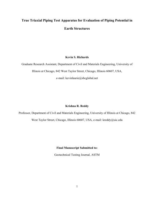
1-inch (2.54 cm)

Water FlowControl PanelPressurized WaterSource VesselTrue Triaxial CellPressurizedReceiving VesselInlet-OutletPressureControlPanelAir Bladder Pressure Control PanelTo Air CompressorKeyAir LineWater Line

To AirCompressorTo Pressurized WaterSourceTo Triaxial Cellor PressurizedWater Source(when needed)Water TrapTo AirBladderPressureControlPanel0-90 psi0-15psiWater TrapToPressurizedReceivingVessel0-15psiVacuumGenerator(-) 0-10 psi

1‐inch (2.54 cm) 1‐inch (2.54 cm) 1‐inch (2.54 cm)Fig. 4a – Inlet-Outlet Pressure Control Panel Fig. 4b – Inlet Flow-Control Panel Fig. 4c – Air Bladder Control Panel

Triaxial CellTo PressurizedWater SourceBypassGranular DeairingFilterMicro-poreFilterLow FlowRegulatorHigh FlowRegulator

Air Bladder(Inflated)Neoprene PadSteel PlatesFlexibleMembrane¼ inch NPTMale Fitting

T-fitting forDifferentialPressure GageQuick-release FittingsPressureTransducerTurbidimeterBall ValvesOutlet Valve TreeInlet Valve Tree

Outlet Tube880 nmDetectorOutlet TubeWiringPVC Nipple880 nm LEDEmitterAcrylicFilled BoxEnd View Side View

Soil Test No. 3356Soil QS305Outlet Pressure (kPa)Outlet, Inlet Pressure (kPa), Differential Pressure (cm)252015104321Turbidity (volts), Outflow (cm3/sec)Inlet Pressure (kPa)Differential PressureTurbidity (volts)5010 per. Mov. Avg. (Outflow(cm3/sec))00 0.001 0.002 0.003 0.004 0.005 0.006 0.007 0.008 0.009‐1Elapsed Time (hr:min:sec)

1.21Vcrit ‐Critical Velocitycm/sec0.80.6y = ‐0.007x 2 + 0.0807x + 0.7882R² = 0.7836vcritPoly. (vcrit)0.40.200 2 4 6 8 10 12ς‐Rate of Change of Inflow(ml/min)/min

1.401.201.00Critical Velocity, v critcm/sec0.800.60y = 0.024x + 0.974R² = 0.7196Seepage Angle vs vcritLinear (Seepage Angle vs vcrit)0.400.200.00‐15 ‐10 ‐5 0 5 10 15Seepage Angle β (degrees)