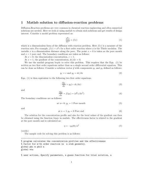
1 Matlab solution to diffusion-reaction problems

The boundary condition at x = 0 (pore mouth) depend on the bulk concentrations of A and B. Theboundary condition at x = 1 (pore end) is the no flux condition for both A and B.The solution vector y has size of four and consists of:⃗y =⎛⎜⎝y 1 = c Ay 2 = dc A /dxy 3 = c By 4 = dc B /dx⎞⎟⎠ (10)The system is now formulated as four first order ODEs for the four components of the solutionvector and solved by bvp4c in exactly the same way. Details are left out as homework problem.An important consideration in this type of problem is how the selectivity is affected by porediffusion. The yield of B is defined as:Yield = flux of B out of the pore mouth / flux of A into the porewhich can be stated as:Yield = −(dc b /dx) x=0 /(dc a /dx) x=0 (11)The relative concentration gradients of A and B at the pore mouth determines the local yield of B.A smaller catalyst size is favorable to B production. A larger particle traps B in the interior of thepores allowing it to react further and form C. This reduces the yield.Maximum yield = (k 1 C A0 − k 2 C B0 )/k 1 C A0 which is also equal tomaximum yield = 1 − k 2C B0k 1 C A0with C A0 and C B0 representing the pore mouth concentrations.Pore diffusion resistance causes the yield to decrease from the above maximum value. Maximumyield is realized only at low values of the Thiele parameters.Example simulated with matlab for a particular case illustrates this point. ).Consider φ 1 = 2 and φ 2 = 1. Also c a0 = 1 and c b0 = 0 which may correspond to the inlet of thereactor (with no recycle), Yield is found as 0.8067.Now let the catalyst size be reduced to one half the original size. Then both φ 1 and φ 2 decrease.The new value of yield is found to be 0.8764. Maximum yield is 1 for both of these cases. The porediffusion resistance has decreased the yield but the reduction is even more for the larger particles..Students should verify these using matlab.2 Asymptotic Solution to diffusion-reaction problemsFor a single non-linear reaction problem, a solution can be obtained analytically for large values ofThiele modulus. This asymptotic solution can then be used to define a generalized Thiele modulusand can be extended to obtain approximate analytical solutions even for low Thiele modulus. Thisavoids solution by numerical methods and is useful in reactor design where repeated calculation ofthe effectivness factor at different points in the reactor is often needed. The procedure is illustratedbelow.Consider a model problem represented as:d 2 cD e = f(C) (12)dx2 3

where f(C) is the rate (dimensional) of consumption of species. The order of the differential equationcan be reduced by one by using the transformation p = dC/dx. Noting thatwe find that Eq. (12) can be written asd 2 Cdx 2= p dpdCD e p dp = f(C) (14)dCThe above equation can be solved by separation of variables. Two limits are needed to obtainthe value of the concentration gradient at the surface, p s . At the pore end, the value of the gradientp is zero. Also for large values of Thiele modulus the concentration drops to nearly zero at someinterior point in the catalyst. Hence the concentration can be set as zero at the pore end. Thus wecan set C = 0 at p =0 as one of the limits for integration of Eqn. (14). Let the surface gradient bedesignated as p s and the concentration at the surface as c s . This sets another limit for integrationof Eqn 13 which can be now be written as:Integrating and rearranging∫ psD e pdp =0∫ Cs0(13)f(C)dC (15)[ ( ∫ 1/2 Csp s = − 2/D e f(C)dC)](16)0The minus sign is used for the square root since the concentration is decreasing with increase in x.The effectiveness factor is given by the ratio of the actual rate to that based on surface concentration.Actual rate = − D e p s S p (17)by Ficks law applied at the surface. Hence the effectiveness factor is given by:η = −D e p s S p /V p f(C s ) (18)Using the Eq. 16 for p s we find[ ∫ 1/2 Csη =(S p /V p )f(C s ) 2D e f(C)dC](19)The above result is applicable for any kinetics provided we are in the asymptotic region. For a firstorder reaction η =1/Λ for large Thiele modulus. In order to make the results in the same format itis convenient to define a Thiele modulus for any kinetics as:[ ∫ −1/2 CsΛ=(V p /S p )f(C s ) 2D e f(C)dC](20)which is known as the generalized Thiele modulus. Now we have η =1/Λ for any kinetics but onlyin the asymptotic case. The expression for η is now generalized as:η = tanh(Λ)(21)ΛThe above expression is strictly valid only in the asymptotic region where tanh(Λ) tend one but isused for the entire range of Λ values as an approximate solution.004

5 Stefan-Maxwell model for multicomponent diffusionMass transport in isothermal multicomponent systems in the gas phase is described by the followingconstitutive equation.− dC n idx =∑ y j N i − y i N j(28)D ijj=1where n is the number of components and D ij is the binary pair diffusivity in the gas phase.For porous catalysts the equation is modified by including both Knudsen and bulk diffusion.− dC idx = N i+D Ke,in∑j=1y j N i − y i N jD ij,e(29)The mass balance for a differential control volume (for a 1-D slab geometry) givesnrdN idx = ∑ν ji r j (30)where the RHS is the total rate of production of species i from the various reactions. The term r j isthe rate function for the j-th reaction which is the function of the local concentrations of the variousspecies. Eqn. (29 and 30 have to be integrated together now.Note that Eqn. 29 can be written in terms of the component partial pressures as:− 1R G Tdp idx = N i+D Ke,iin∑j=1p j N i − p i N jP t D ij,e(31)where P t is the total pressure and R G is the gas constant. Since the rates of reactions are usuallycorrelated as a function of partial pressures, the above form is often more convienient. The viscouscontribution to flow is neglected in these equations. It does not mean that the catalyst pellets areisobaric; pressure gradients can exist in the pellets and they are implicitly accounted for by the useof the constitutive equations in terms of the partial pressures rather than in terms of componentmole fractions.A structure of a matlab program for solving these equations is presented here.function StefanMaxwell ()% program calculates the concentration profiles and the effectiveness% factor based on Stefan-Maxwell model.% 3-07-05 written by P. A. Ramachandran% test problem 1 in the paper by Haynes% user actions, Specify parameters, a guess function for trial solution, a% function odes to define the set of first order differential equations% and a function bcs to specify the boundary conditions.% also define rate in the function ratemodel.global ns neqns = 4 % four speciesneq = 8 % 4*2 equations% Eight variables Y(1) to y(4) are the concentrations of CO, H2O, CO2 and7

% H2, y(5) to y(8) are the flux values.% parameters used are as follows:global temp pressureglobal ctottemp = 400+273.;pressure = 25.0 ; % atmRgas = 82.06 % gas contant in cm^3 atm /g-mole Kctot = pressure/Rgas/temp; % total concentration mole/c.c% surface (pore mouth) mole fractionglobal ysys(1) = 0.1; ys(2) = 0.6; ys(3) = 0.08; ys(4) = 0.22 ;ys = ys * ctot % surface molar concentrations.% rate and other parametersglobal k rhop Keqk = 2.05e-04 ;rhop = 1.84 ;Keq = 12.0% diffusion parameters; dk = knudsen ; db = binary pair (a matrix)global dk dbdk(1) = 0.00649;dk(2) = 0.00494 ;dk(3) = 0.0098;dk(4) = 0.0231;% **** add db values for binary pairs% catalyst propertieslength = 0.1588 ;rate_s = reactionrate(ys) ; % rate based on surface valuesnmesh = 21 % intial meshnplot = nmesh ; % meshes for plotting the result.% solution block.x = linspace ( 0, 1, nmesh ) ;solinit =bvpinit ( x , @guess ) % trial solution generated by guess functionsol = bvp4c (@odes, @bcs, solinit) % bvp solved,% post processing. plot concentration profiles, find etax = linspace ( 0, length, nplot) ;y = deval(sol, x) ;% concentration profiles of various components.y(1,:)y(3,:) ;y(2,:)y(4,:) ;plot ( x, y(1,:) , ’-+’ ) ;% hold on ; plot (x, y(2,:), ’-+’ ) % these are plotted.% flux values for the four species.y(5,1)8

y(6,1)y(7,1)y(8,1)rate_seta = y(5,1)/rate_s /0.1588%______________________________________________________function yinit = guess (x)global phi m phi2 nglobal ysglobal k rhop Keq% find rate based on surface values and use it as trial value for flux%rate =rhop* k * ys(1)^0.9 * ys(2)^0.3 * ys(3)^(-0.6) * (1.- ys(3) * ys(4)/Keq/ys(1) /ys(2) )rate= reactionrate(ys) ;yinit = [ys(1)ys(2)ys(3)ys(4)-rate-rateraterate ] ; % guess values here%-------------------------------------------------------function dydx = odes ( x, y )global ns neqglobal ctotglobal k rhop Keqglobal dk dbrate = reactionrate(y);% bulk diffusion terms to be added. Currently set as zerobulkterm = zeros (ns,1);dydx = [- y(5) /dk(1) + bulkterm(1)- y(6)/dk(2)-y(7)/dk(3)-y(8)/dk(4)-rate-rateraterate ] ;%-----------------------------------------------------------function res = bcs ( ya , yb)global a0 b0global ysres = [ ya(1) - ys(1)ya(2) - ys(2)ya(3) - ys(3)ya(4) - ys(4)yb(5)9

yb(6)yb(7)yb(8) ] ;%___________________________________________________________________function ratemodel = reactionrate(y)global k rhop Keqglobal temp pressureglobal ctotp = y*82.06*temp % species partial pressuresratemodel =rhop* k * p(1)^0.9 * p(2)^0.3 * p(3)^(-0.6) * (1.- p(3) * p(4)/Keq/p(1) /p(2) ) ;10

6 Temperature EffectsThe simultaneous transport of heat and mass in a porous catalyst can be represented by the followingset of equations.d 2 CD e = f(C, T ) (32)dx2 d 2 Tk e =(∆H)f(C, T ) (33)dx2 where k e is the effective conductivity of the catalyst and ∆H is the heat of reaction. The local rate(of disappearance) f(C, T ) is now a function of both the pore concentration and the temperature atany point in the pellet.The boundary conditions are specified as follows: No flux condition is imposed at the pore end(x = 0) for both heat and mass.at x =0 dC/dx =0; dT/dx =0At the pore mouth (x = L) the flux into the pellet must match the transport through the gas film.This leads to the following boundary conditions.For mass transport( ) dTD e = k m (C g − C x=L )dxx=LFor heat transport( ) dTk e = h(T g − T x=L )dxx=LThe equations can be put in terms of dimensionless variables by scaling the concentration andtemperature by reference values. The bulk concentration and temperature can be used as thereference values if the particle scale model is being analyzed. For reactor scale models, the inlet feedconditions can be used as reference.The dimensionless mass and heat transport equations are then as follows:d 2 cdξ 2 = f(C ref,T ref )L 2[f ∗ (c, θ)]) (34)D e C refwhere ξ is dimensionless distance x/L and f ∗ is a dimensionless rate defined as:f ∗ = f(C, T )/[f(C ref ,T ref )]The first term on the RHS of 34 can be identified as a Thiele parameterLet φ 2 = f(C ref,T ref )L 2D e C refThen the mass balance equation is:d 2 cdξ 2 = φ2 f ∗ (c, θ) (35)The heat balance equation can be represented as:d 2 θdξ 2 = −βφ2 f ∗ (c, θ) (36)11

where β is the dimensionless parameter (thermicity group) defined as:β = (−∆H)D eC refk e T ref(37)Note the β takes a positive value for exothermic reactions and a negative value for endothermicreactions.The boundary conditions can be normalized as:at ξ =0 dc/dξ =0; dθ/dξ =0and the conditions at ξ = 1 can be related to the Biot numbers for heat and mass( ) dc= Bi m (c g − c s ))dξs( ) dθ= Bi h (θ g − θ s ))dξswhere the subscript s is used for the ξ = 1 i.e,. the surface values. Here we defineandBi m = k m L/D eBi h = hL/k eThe magnitude of the internal temperature gradient can be assessed by combining the above twoequations without even actually solving the equations. The mass and heat transport equations 35and 36 can be combined as:d 2 θdξ 2 + β d2 cdξ 2 (38)Hence the integration of the above equation twice leads toθ − θ s = β(c s − c) (39)The maximum value of the temperature occurs for an exothermic reaction when the center concentrationdrops to zero. This occurs in the strong pore diffusion resistance for mass transfer. Hencean estimate of the internal gradients is:Max θ c − θ s = βc s = O(β) (40)where θ c is the center temperature and the symbol O means ’of the order of’.Also the magnitudes of the external gradients can be estimated by the following procedure: Herewe introduce the overall effectiveness factor η 0 defined as: η 0 = actual rate / rate based on referenceconditionsRate of transport to the surface is equal to S p k m (C g − C s )Rate of reaction is V p f(C ref ,T ref )η 0 .Equating the two and using the dimensionless groups we find as estimate of the external concentrationgradients.c g − c s = φ2 η 0(41)Bi m12

Note that φ 2 η 0 is the same as the Weisz modulus and can be directly calculated if the measureddata is available. The value of η 0 need not be explicitly evaluated in order to use the above equationfor diagnostic purposes.φ 2 η 0 =(−R measured )L 2 /(D e C ref ) (42)Similar analysis equating the heat transport in the film to the total heat released from thereaction leads to an estimate the film temperature difference.θ s − θ g = βφ2 η 0(43)Bi hThe above relations enables a rapid determination or the relative importance of external andinternal temperature gradients. It can be, for instance, used to determine if the pellet is operatingunder near isothermal conditions or whether a temperature correction to the data is necessary.The temperature rise in the pellet can be assessed as follows: Combining 41 and 43 we find:( )θ c − θ s = c g β 1 − φ2 η 0(44)Bi mwhich is a closer estimate of the pellet temperature rise than the earlier equation based on thesurface concentration.7 Numerical SolutionsNumerical solution for a first order reaction is indicated in this section. The dimensionless rate fora first order reaction can be expressed as:f ∗ = c exp[γ(1 − 1/θ)] (45)where γ = E/R g T ref . The governing equations and the boundary conditions shown in the earliersection are summarized for convenience here: The mass balance:The heat balance:The boundary conditions are:d 2 cdξ 2 = φ2 c exp[γ(1 − 1/θ) (46)d 2 θdξ 2 = −βφ2 c exp[γ(1 − 1/θ) (47)at ξ =0 dc/dξ =0; dθ/dξ =0and ξ =1( ) dc= Bi m (c g − c s ))dξs( ) dθ= Bi h (θ g − θ s ))dξsFor the particle problem (local particle scale model) we set c g and θ g as one.We find that even for this simple first order reaction, the overall effectiveness factor is a functionof five parameters: φ, β, γ, Bi m and Bi h .13