An Efficient, and Fast Convergent Algorithm for Barrier Options

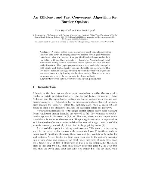
An Efficient, and Fast Convergent Algorithm forBarrier OptionsTian-Shyr Dai 1 and Yuh-Dauh Lyuu 21. Department of Information and Finance Management, National Chiao-Tung University, 1001 TaHsueh Road, Hsinchu, Taiwan 300, ROC. E-mail:d88006@csie.ntu.edu.tw. He was supported byNSC grant 94-2213-E-033-024.2. Department of Computer Science & Information Engineering, National Taiwan University.Abstract. A barrier option is an option whose payoff depends on whetherthe price path of the underlying asset ever reaches certain predeterminedprice levels called the barriers. A single- (double-) barrier option is a barrieroption with one (two, respectively) barrier(s). No simple and exactclosed-form pricing formula for double-barrier options has been reportedin the literature. This paper proposes a novel tree model that can priceboth single- and double-barrier options efficiently and accurately. Thistree model achieves the high efficiency by combinatorial techniques andnumerical accuracy by hitting the barriers exactly. Numerical experimentsare given to verify the superiority of our method.Keywords: barrier option, combinatorics, option pricing, tree1 IntroductionA barrier option is an option whose payoff depends on whether the stock pricereaches a certain predetermined level (the barrier) before the maturity date.A double- and the single-barrier options are barrier options with two and onebarriers, respectively. A knock-in barrier option comes into existence if the stockprice reaches the barrier(s) before the maturity date, while a knock-out oneceases to exist if the stock price reaches the barrier(s) before the maturity.When the payoff functions for the single barrier options follow some standardforms, analytical pricing formulas are derived in [8]. The valuation of doublebarrieroptions is discussed in [5, 11, 6]. However, there are no simple, exactclosed-form formulas for these options. The pricing formula can be expressed asan infinite series of cumulative normal distributions. Although truncation of thisseries is necessary numerically, it can lead to large pricing errors [6].A tree model is popular for pricing barrier options. This research is interestingsince it can price barrier options with nonstandard payoff functions, such aspower payoff functions. However, there may not be closed-form formulas forsuch options. A tree divides the time span from now to the option’s maturityinto n time steps and simulates the stock price discretely at each step. Takethe 3-time-step CRR tree [2] illustrated in Fig. 1 as an example. Let the stockprice at time step 0 be S 0 . From an arbitrary node with price S ′ , the CRR treesays that the stock price after one time step equals S ′ u (the up move) with

Efficient Algorithms for Barrier Options 7A 1 and hitting L before reaching B equals to the number of paths moving fromA 2 to B. Thus the number of paths moving from A to B and reaching H atleast once before reaching L is equal to the number of paths moving from A 2 toB. Assume that x up moves and y down moves are required to move from A 2to B. Thuswehavex + y = n and x − y = a − b +2s. Wegetx = n+a−b+2s2bysolving the above equations. So the answer to the aforementioned problem is( n )n+a−b+2s2for even, non-negative n + a − b. (5)Note that a path counted by Eq. (5) may hit L first before hitting H. The pointis that among the hits, one hit of H must appear before one hit of L.The problem of counting the number of paths that will hit either H or Lbefore arriving at B is now within reach. First, a function f is constructedto map each path to a string. This string contains the information about thebarrier hitting sequence. For example, f(ÂB) =HHL since ÂB hits H twicebefore hitting L. Next, we define α i as the set of paths whose f value containsi{ }} {H + L + H + ···. L + and H + denote a sequence of Ls andHs, respectively. Obviously,ÂB belongs to set α 1 and set α 2 . Similarly, define β i as the set of pathsi{ }} {whose f value contains L + H + L + ···. Thus the path ÂB belongs to set β 1.Thenumber of elements in set α i and β i can be calculated by repeatedly using thereflection principle. The number of elements in each set is listed as follows:⎧ ()n⎪⎨ n+a+b+(i−1) s for odd i| α i | = (2 )n⎪⎩ n+a−b+is for even i2⎧ ()n⎪⎨ n−a−b+(i+1) s for odd i| β i | = (2 )n⎪⎩ n−a+b+is for even i2Note that each path that hits the barrier may belong to more than one set. Forexample, ÂB belongs to α 1, α 2 ,andβ 1 . The inclusion-exclusion principle is thenapplied to calculate the number of paths that moves from A (with coordinate(0, −a)) to B (n, −b) and that hit either H or L at least once as follows:⌈∑n s ⌉N(a, b, s) = (−1) i+1 (|α i| + |β i|). (7)i=1The Pricing AlgorithmThe construction of the pricing algorithm can be divided into several differentcases. For some degenerate cases like S 0 ≤ L, S 0 ≥ H, andX ≥ H,the value of a knock-in double-barrier option can be proved to equal the valueof a vanilla call option. These degenerate cases can be directly priced by anyanalytical or numerical method that price a vanilla call option. So we furtherfocus on the case L

8 Dai and LyuuPrice level2h( Sn 0u )n−2h( S0u)H0 n Time step( S 0)2h − n2h − 2lLs ≡ 2l− 2h( S u0n−2l)2h − 2n( Sn 0u− )Fig. 5. Put a CRR Tree on a Lattice. The coordinate of the root node of the CRRtree is (0, 2h − n). The values in parentheses denote the stock prices.Now we analyze the value contributed by a price path that reaches N(n, j).The probability for this path is p n−j (1−p) j . The payoff at N(n, j)is(S 0 u n−j d j −X) + . Thus the value contributed by this path is p(j) ≡ e −rT p n−j (1−p) j (S 0 u n−j d j −X) + , if this price path hits the barrier. Note that the value contribution byN(n, j) isV (j) ≡ ( n j )p(j) ifN(n, j) isaboveH or below L (inclusive). This isbecause all the price paths that reach N(n, j) must also hit the barrier.The pricing algorithm can be divided into two following cases. For convenience,the term“terminal node” refers to the node of the tree at maturity date.Case 1. Lh), between X and H. The number of paths that reach one ofthe barriers before reaching N(n, j) isN(n − 2h, 2j − 2h, 2l − 2h) (see Eq. (7)).The value contributed by such a path is p(j). Therefore, the value contributedby node N(n, j) isN(n − 2h, 2j − 2h, 2l − 2h)p(j). The first part of the optionvalue is P 0 ≡ ∑ a−1j=h+1N(n − 2h, 2j − 2h, 2l − 2h))p(j). The second part of theoption value is computed by accumulating the values contributed by the terminalnodes, says N(n, i) (0≤ i ≤ h), above the barrier H (inclusive). The valuecontributed by N(n, i) isV (i). Therefore, the second part of the option value isP 1 = ∑ hi=0 V (i). The value of a knock-in double-barrier call option is P 0 + P 1 .Case 2. X ≤ L: The option value is decomposed into three parts: (1) the valuecontributed by the terminal nodes between L and H, (2) the value contributedby the terminal nodes above H (inclusive), and (3) the value contributed by theterminal nodes between L (inclusive) and X. The first part of the option valueis expressed as P 0 ′ ≡ ∑ l−1j=h+1N(n − 2h, 2j − 2h, 2l − 2h)p(j). The second partof the option value equals P 1 . The third part is computed by accumulating thevalues contributed by the terminal nodes, says N(n, k) (l ≤ k

Efficient Algorithms for Barrier Options 95 Experimental ResultsWe first compare the performance among the TB tree, Lyuu’s algorithm [7],and the Ritchken’s trinomial tree [10] in Table 1. All programs are run on aPentium-4 2.8GHz computer. Note that Lyuu’s algorithm oscillates significantly.Both Ritchken’s trinomial tree and the TB tree converge monotonically to thetrue value 5.9968. But the TB tree can achieve each level of accuracy with fewercomputational time than the Ritchken’s trinomial tree. Thus we conclude thatthe TB tree is superior to both Lyuu’s and the Ritchken’s approaches.Table 1. Convergence Rate for Pricing a Down-and-Out Single-Barrier Option.Ritchken Lyuu TBTime (sec) n Value n Value n Value0.001 100 5.9997 1000 6.1002 500 5.99800.004 200 5.9986 4000 6.1998 2000 5.99720.016 400 5.9980 16000 6.0829 8000 5.9969The initial stock price is 95, the exercise price is 100, the risk-free rate is 10% perannum, the volatility of the stock price is 25%, the time to maturity is 1 year, and thebarrier is 90. Time denotes the computational time in seconds. n and Value denotes thenumber of time steps and the pricing result of each tree model.The TB tree can accurately solve the barrier-too-close problem for pricingdouble-barrier options while AMM can not as illustrated in Table 2. Level denotesthe AMM level. The number of steps of AMM is determined by the AMMlevel. The Inner Barrier and the Outer Barrier denote the results computedby moving the upper barrier (120) to the inner barrier and the outer barrier,respectively. Note that AMM undervalues the option if the upper barrier movesdown to the inner barrier and overvalues the option if the upper barrier movesup to the upper barrier. Each pricing result of the TB tree is properly selected sothe number of steps of the TB tree is approximately equal to that of the AMM.Obviously, the TB tree provides more accurate results than the AMM.6 ConclusionThe TB tree that can efficiently and accurately price barrier options is proposedin this paper. It is mainly composed of the CRR tree so the computation canbe speeded up by combinatorial techniques. It produces accurate pricing resultssince it has a layer to coincide with each barrier. Numerical results show thatthe TB tree are superior to other existing approaches.References1. Boyle P., and Lau, S. “Bumping Against the Barrier with the BinomialMethod,” Journal of Derivatives, 1 (1994), pp. 6–14.

10 Dai and LyuuTable 2. Convergence Rate Comparison between AMM and the TB tree.AMMTBLevel n Inner Barrier Outer Barrier n Value2 671 0.000001 0.000015 655 0.0000031 2686 0.000001 0.000005 2625 0.000003The initial stock price and the exercise price is 100, the risk-free rate is 10%, thevolatility of the stock price is 30%, the time to maturity is 1 year, and the two barriersare 99.5 and 120, respectively. The pricing results of the TB tree converge to 0.000003.2. Cox J., Ross, S., and Rubinstein, M. “Option Pricing: A Simplified Approach.”Journal of Financial Economics, 7 (1979), pp. 229–264.3. Derman, E., Kani, I., Ergener, D., and Bardhan, I. “Enhanced NumericalMethods for Options with Barriers,” Working Paper, Goldman Sachs. (1995).4. Figlewski, S., and Gao, B. “The Adaptive Mesh Model: A New Approach toEfficient Option Pricing.” Journal of Financial Economics, 53 (1999), pp. 313–351.5. Geman H., and Yor, M. “Pricing and Hedging Double-Barrier Options: A ProbabilisticApproach.” Mathematical Finance, 6 (1996), pp. 365–378.6. Luo, L. “Various Types of Double Barrier Options.” Journal of ComputationalFinance, 4 (2001), pp. 125–138.7. Lyuu Y.D. “Very Fast Algorithms for Barrier Option Pricing and the BallotProblem.” Journal of Derivatives, 5 (1998), pp. 68–79.8. Merton, R. “Theory of Rational Option Pricing.” Bell Journal of Economicsand Management, 4 (1973), pp. 141–183.9. Reiner, E. and Rubinstein, M. “Breaking Down the Barriers.” Risk, 4 (1991),pp. 28–35.10. Ritchken, P. “On Pricing Barrier Options.” Journal of Derivatives, 3 (1995),pp. 19–28.11. Sidenius, J. “Double Barrier Options: Valuation by Path Counting.” Journal ofComputational Finance, 1 (1998), pp. 63–79.AValidity of Risk-Neutral ProbabilitiesDefine det = (β − α)(γ − α)(γ − β), det u =(βγ + Var)(γ − β), det m =(αγ +Var)(α − γ), and det d =(αβ + Var)(β − α). Then Cramer’s rule applied toEq. (2)–(4) gives P u = det u /det, P m = det m /det, and P d = det d /det. Notethat det < 0 because α>β>γ. To ensure that the branching probabilitiesare valid, it suffices to show that P u , P m , P d ≥ 0. As det < 0, it is sufficientto show det u , det m , det d ≤ 0 instead. Finally, as α > β > γ, it suffices toshow that βγ +Var≥ 0, αγ +Var≤ 0, and αβ +Var≥ 0 under the premiseβ ∈ [−σ √ ∆t, σ √ ∆t). Indeed,βγ +Var=β 2 − 2βσ √ ∆t + σ 2 ∆t ′ ≥ β 2 − 2βσ √ ∆t + σ 2 ∆t =(β − σ √ ∆t) 2 ≥ 0,αγ +Var=β 2 − 4σ 2 ∆t + σ 2 ∆t ′ ≤ β 2 − 4σ 2 ∆t +2σ 2 ∆t = β 2 − 2σ 2 ∆t ≤ 0,αβ +Var=β 2 +2βσ √ ∆t + σ 2 ∆t ′ ≥ β 2 +2βσ √ ∆t + σ 2 ∆t =(β + σ √ ∆t) 2 ≥ 0,as desired.