(SCAD) regularization for compressed sensing MRI Using ... - PINLAB

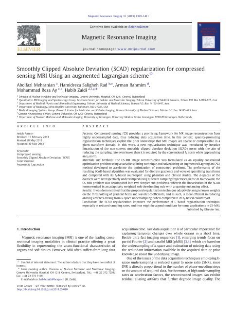
1400 A. Mehranian et al. / Magnetic Resonance Imaging 31 (2013) 1399–1411reduced SNR and residual artifacts, in fact, arise from the illconditioningof the inverse problems encountered in this context [5].Regularization and explicit incorporation of prior knowledge duringreconstruction of MR images are efficient ways to improve theconditioning of the problem and thus to penalize unsatisfactory andnoisy solutions. Several regularization schemes have been assessedin this context. Tikhonov regularization suppresses noise andartifacts by favoring smooth image solutions [6–8].The truncatedsingular value decomposition attempts to reduce noise by truncatingsmall singular values on the assumption that noise amplification isassociated with small singular values of solution [6,9]. Bothregularizations are based on l 2 norm minimization and tend to blurthe details and edges in the estimated image [6,10]. Recentdevelopments in compressed sensing have introduced sparsityregularization techniques, which have garnered significant attentionin MR reconstruction from highly undersampled k-spaces. In fact, CS-MRI reduces noise and aliasing artifacts by exploiting the priorknowledge that MR images are sparse or weakly sparse (compressible)in spatial and/or temporal domains [11,12], in a giventransform domain such as wavelets, Fourier, discrete gradients[11,13] or in learned dictionaries [14,15]. By establishing a direct linkbetween sampling and sparsity, CS theory provides an alternativesampling criterion to conventional Shannon–Nyquist theory [16,17].According to this theory, it is possible to accurately recover theunderlying signal or solution from the data acquired at samplingrates far below the Nyquist limit as long as i) it is sparse or has asparse representation in a given transform domain and ii) thesampling pattern is random or such that the aliasing artifacts areincoherent (noisy-like) in that domain [17,18].Sparsity regularization aims at finding a solution that has thesparsest representation in a given sparse transform domain. In thisregard, the l 0 norm is an ideal regularizer (or prior), which counts thenumber of non-zero elements of the solution [19]. However, thisnon-convex prior results in an intractable and non-deterministicpolynomial-time hard (NP-hard) optimization problem. For thisreason, the l 1 norm has been widely used as a convex surrogate tothe l 0 norm and has gained popularity in conjunction with wavelet[20,21] and discrete gradient transforms [22]. The latter is known astotal variation (TV) regularization [23–26] and has been shown tooutperform l 2 -based regularizations in CS-(p)MRI [27,28]. The l 1 -based regularizations; however, show a lower limit in the requiredsampling rate and hence in the maximum achievable accelerationrate [29]. In addition, the l 1 norm is known to be biased due to overpenalizinglarge sparse representation coefficients [30]. To furtherreduce the sampling rate and approach l 0 norm minimization,Candes et al. [30] proposed a reweighted l 1 norm minimization inwhich the sparsity induced by the l 1 norm is enhanced by theweighting factors that are derived from the current estimate of theunderlying solution. This approach has been successfully applied inCS-(p)MRI [31–33]. Furthermore, non-convex priors homotopicallyapproximating the l 0 norm have also been studied showing theimproved performance of the resulting regularization techniques inthe recovery of strictly sparse signals [19,34,35]. However, MRimages are usually compressible rather than sparse, hence it isdesirable to exploit the sparsity-promoting properties of both l 1 andl 0 norm minimizations [36]. To improve the properties of l 1 andpseudo l 0 norms in terms of unbiasedness, continuity and sparsity,Fan and Li [37] proposed a non-convex prior called smoothly clippedabsolute deviation (SCAD) norm in the context of statistical variableselection. This norm has been designed to not excessively penalizelarge valued coefficients as in the l 1 norm and at the same timeapproaching an l 0 norm. Teixeira et al. [38] have previously studiedthe SCAD regularization for sparse signal recovery using a secondordercone optimization method. In this work, we employed, for thefirst time, the SCAD regularization with discrete gradients andwavelet transforms in the context of CS-MRI and solved the resultingproblem using variable splitting and augmented Lagrangian (AL)methods. In the AL framework, the optimization problem is reducedto simpler sub-problems, leading to an improved convergence rate incomparison with state-of-the-art and general purpose optimizationalgorithms [39,40]. In this framework, the linearization of the SCADnorm resulted in a weighted soft thresholding rule that exploits theredundant information in image space to adaptively threshold thegradient fields and wavelet coefficients and to effectively reducealiasing artifacts. In this study, we compared the performance of theproposed SCAD-based regularization with the conventional l 1 -basedapproach using simulation and clinical studies, where k-spaces wereretrospectively undersampled using different sampling patterns todemonstrate the potential application of the proposed method in CS-MR image reconstruction.2. Materials and methods2.1. TheoryFor a single-coil CS-MRI, we formulate the following CSacquisition model:y ¼ ΦFx þ nwhere γ∈C M is the undersampled k-space of the underlying MRimage, x∈R N , contaminated with additive noise n∈C M . F∈C N × N is aFourier basis through which x is being sensed and Φ∈R M × N is asampling matrix that compresses data to M b N samples. The matrixA = ΦF is often referred to as sensing or Fourier encoding matrix.The direct reconstruction of x from y (by zero-filling the missing dataand then taking its inverse Fourier transform) results in aliasingartifacts, which is attributed to the ill-conditioning of matrix A. Asaresult, regularization is required to regulate the solution spaceaccording to a prior knowledge. The solution can therefore beobtained by the following optimization problem:1^x ¼ argim x2 ‖ΦFx−y‖2 þ RðxÞwhere the first term enforces data consistency and the second one,known as regularizer, enforces data regularity. In the CS-MRI context,sparse l 1 -based regularizers have been widely used because the l 1norm is a convex and sparsity promoting norm, thereby the resultingproblem is amenable to optimization using convex programming.NThese regularizers are of the form R(x) =λ‖Ψx‖ 1 = λ ∑ i =1 |[Ψx] i |,where λ > 0 is a regularization parameter controlling the balancebetween regularization and data-consistency and Ψ is a sparsifyingtransform such as discrete wavelet, Fourier or gradient transform.The CS approach makes it possible to accurately reconstruct theimage solution of problem (1), provided that i) the underlying imagehas a sparse representation in the domain of the transform Ψ, i.e.most of the decomposition coefficients are zero, while few of themhave a large magnitude, ii) the sensing matrix A should be sufficientlyincoherent with the sparse transform Ψ, thereby the aliasing artifactsarising from k-space undersampling would be incoherent (noise like)in the domain of Ψ [11,18].2.2. Proposed methodThe sparsity or compressibility of an image solution induced by l 1based regularizers can be increased by introducing a non-convexpotential function, ψ λ , as follows:RðxÞ ¼ ∑ ψ λ j½ΨxŠ ij ½3Ši¼1½1Š½2Š

A. Mehranian et al. / Magnetic Resonance Imaging 31 (2013) 1399–14111403phantoms and clinical datasets. To demonstrate the performance ofSCAD regularization for highly undersampled MR reconstruction, wefirst performed a set of simulated noisy data generated from theanthropomorphic XCAT phantom. In this experiment, the k-space ofa 512 × 512 slice of the XCAT phantom was sampled by 8 equallyspaced radial trajectories as well as a single-shot variable-densityspiral trajectory, respectively corresponding to 98.33% and 98.30%undersampling, with 20 dB complex noise added to k-spaces. For theevaluation of the proposed SCAD-ADMM algorithm with 3D discretegradients, an MR angiography (MRA) dataset in a patient witharterial bolus injection was obtained from Ref. [49]. The dataset hasbeen synthesized from projection data collected for 3 frames persecond for a total of 10 s (31 collected frames) and linearlyinterpolated into 200 temporal frames. In this study, 30 time framesof this dataset (with resolution of 256 × 256) were chosen and their3D k-space was retrospectively undersampled using a stack of 2Dsingle-shot variable-density spiral trajectories, yielding 78.7% undersampling.The performance of the algorithm was further evaluatedwith 2D translation-invariant wavelets using two brain datasets. Atransverse slice of a 3D brain T1-weighted MRI dataset (of the size181 × 217 × 181) was obtained from the BrainWeb database(McGill University, Montreal, QC, Canada) [50], which has beensimulated for 1 mm slice thickness, 3% noise and 20% intensity nonuniformity.The image slice was zero-padded to 256 × 256 pixelsand its k-space was retrospectively undersampled by a variabledensityrandom sampling pattern with 85% undersampling. Finallyin clinical patient study, a Dixon MRI dataset was acquired on aPhilips Ingenuity TF PET–MRI scanner (Philips Healthcare, Cleveland,OH). The MRI subsystem of this dual-modality imaging system isequipped with the Achieva 3.0 T X-series MRI system. A whole bodyscan was acquired using a 16-channel receiver coil and a 3D multiecho2-Point FFE Dixon (mDixon) technique with parameters: TR =5.7 ms, TE1/TE2 =1.45/2.6, flip angle =10º and slice thickness of2 mm, matrix size of 480 × 480 × 880 and in plane resolution of0.67 mm × 0.67 mm. From this sequence, in-phase, out-of-phase,fat and water (IP/OP/F/W) images are reconstructed. For thecomparison of SCAD- and l 1 -based wavelet regularizations, arepresentative image slice of OP image was zero-padded to512 × 512 pixels and its k-space was retrospectively undersampledby the Cartesian approximation of radial trajectory with 83%undersampling. Note that the k-spaces of the studied datasetswere obtained by forward Fourier transform of the image slices.All of our CS-MR reconstructions were performed in MATLAB2010a, running on a 12-core workstation with 2.40 GHz Intel Xeonprocessors and 32 GB memory. The improvement of image qualitywas objectively evaluated using peak signal to noise ratio (PSNR)and mean structural similarity (MSSIM) index, [51] between theground truth fully sampled image, x⁎ and the images reconstructedby l 1 - and SCAD-based regularizations, x. The PSNR isdefined as:0maxjx 1i jPSNR x; x 1≤i≤N¼ 20 log 10 BqffiffiffiffiffiffiffiffiffiffiffiffiffiffiffiffiffiffiffiffiffiffiffiffiffiffiffiffiffiffiffiffiffiC@ 1N ∑N i¼1jx i −x ij 2 AMSSIM, which evaluates both nonstructural (e.g., intensity) andstructural (e.g., residual streaking artifacts) deviations of an imagefrom its reference image, is given by:SSIM x; x ¼ð2μ x μ x þC 1 Þð2σ xx þC 2 Þ μ 2 x þ μ x 2 þC 2 1 σx þ σ x 2 þC 2MSSIM x; x ¼ 1 LX Ll¼1SSIM x l ; x lwhere the mean intensity, μ and standard deviation σ, ofx and x⁎and their correlation coefficient σ xx* , are calculated over L localimage patches. The constants C 1 =(K 1 D) 2 and C 2 =(K 2 D) 2 areintroduced to avoid instability issues, where D is the dynamic rangeof pixel values. K 1 = 0.01 and K 2 = 0.03 according to Ref. [51].Based on this metric, a perfect score, i.e. MSSIM (x, x⁎) =1 isachieved only when the image x is identical to the ground truthimage x⁎. In addition, the reconstructed images were qualitativelycompared through visual comparison and intensity profiles. In allreconstructions, a tolerance of η =1×10 −4 was used in Algorithm 1to declare the convergence of the algorithms.Fig. 2. Reconstruction of the XCAT phantom through zero-filling, gradient-based l 1 and SCAD ADMM algorithms from the k-spaces sampled by 8 equally spaced radial Fouriertrajectories (top) and a variable-density spiral trajectory (bottom), respectively, corresponding to 98.33% and 98.30% undersampling. The difference images show the deviationsof the reconstructed images from the true fully sampled image.

1404 A. Mehranian et al. / Magnetic Resonance Imaging 31 (2013) 1399–1411Table 1Summary of the peak signal-to-noise ratio (PSNR) and mean structural similarity (MSSIM) performance of the studied algorithms in CS-MRI with respect to fully sampled(reference) images.Dataset PSNR (dB) SSIM Iterations | CPU time/Iter. (s)Zero-Filling L1 SCAD Zero-Filling L1 SCAD L1 SCADXCAT (Radial) 17.66 26.03 35.89 0.21 0.83 0.98 2130 0.06 2862 0.08XCAT (Spiral) 14.21 31.41 52.66 0.16 0.84 0.99 2489 0.07 2745 0.08MR Angiogram 24.65 28.32 28.60 0.64 0.69 0.70 94 0.83 138 0.97BrainWeb 14.84 18.52 20.36 0.39 0.59 0.62 335 0.49 354 0.66Brain mDixion 23.76 27.91 29.13 0.31 0.98 0.99 96 1.84 102 2.12The number of iterations and the computation (CPU) time per iteration (in seconds) are also reported.4. Results4.1. CS-MR Image ReconstructionsFig. 2 shows the results of image reconstruction in XCAT phantomfor radial and single-shot variable density spiral trajectories, in firstand second rows, respectively, and compares the images reconstructedby zero-filing, l 1 - and SCAD-based ADMM algorithms withdiscrete gradient sparsifying transform. This figure also shows thedifference images between true and reconstructed images. As can beseen, the proposed regularization technique has efficiently recoveredthe true image and outperformed its TV counterpart in bothFig. 3. (A) Reconstruction of the MR angiogram dataset through zero-filling, gradient-based l 1 and SCAD ADMM algorithms using a 3D stack of a single-shot variable-density spiraltrajectory (78.7% undersampling). The L1 and SCAD images are shown with the same display window. (B) The illustration of k-space undersampling pattern. (C) The comparisonof intensity profiles of reconstructed images along the dash line shown on the true image.

A. Mehranian et al. / Magnetic Resonance Imaging 31 (2013) 1399–14111405Fig. 4. (A) Reconstruction of the BrainWeb phantom through zero-filling, wavelet-based l 1 and SCAD ADMM algorithms using a variable density random sampling (85%undersampling). The L1 and SCAD images are shown with the same display window. (B–C) As in Fig. 3.cases. In this simulation study with extremely high undersampling, theinvolved parameters, i.e. ρ, λ and a, wereheuristicallyoptimizedtoobtain the best case performance of the algorithms. For the radialsampling results, the optimized parameters were set to ρ =0.5,λ =0.03, a =3.7forSCADandρ =0.2,λ = 0.05 for TV. Similarly, in thespiral sampling, the parameters were set to ρ = 0.15, λ = 0.15, a =3.7for SCAD and ρ =0.5,λ = 0.15 for TV. The quantitative evaluation of thealgorithms in terms of PSNR and SSIM index is presented in Table 1.Theresults show that the SCAD regularization significantly improves peaksignal to noise ratio in the reconstructed images and also gives rise to aperfect similarity between the true and the reconstructed images. Itshould be noted that at sufficiently high sampling rate the l 1 -based TVregularization can restore the underlying image as faithfully as theSCAD regularization. However, we purposefully lowered the samplingrate to evaluate the ability of algorithms in CS-MRI from highlyundersampled datasets.In Fig. 3 (A), a representative slice of the reconstructed MRAimages is compared with the fully sampled ground truth. The visualcomparison of the regularized reconstructions shows that both l 1 -based TV and SCAD regularizations have noticeably suppressed noiseand undersampling artifacts in comparison with zero-filling, which isin fact an un-regularized reconstruction. However, a close comparisonof the images reveals that the SCAD regularization results in a higherimage contrast (see arrows), since it exploits the weighting factorsthat suppress regularization across boundaries. Fig. 3 (B) also showsthe k-space trajectory used for undersampling and the intensityprofiles of the reconstructed images along the dashed line shown onthe true image. The profiles also demonstrate that the SCADregularization technique can improve the performance of its TVcounterpart. The algorithms were also quantitatively evaluated basedon PSNR and MSSIM metrics. The results summarized in Table 1further demonstrate the outperformance of the proposed regularizationtechnique. Note that during image reconstruction of this and theother two brain datasets, we first optimized the involved parametersof the ADMM algorithm, i.e. λ and ρ, forl 1 -based regularizations toobtain the best case performance. Then, we optimized the performanceof the SCAD regularization using the same values for the scaleparameter a in Eq. (16). For this dataset, the optimal parameters wereset to λ =1800,ρ = 1.2 and a = 100.Figs. 4 and 5 (A) show the image reconstruction results of thesimulated (BrainWeb) and clinical brain Dixon datasets, respectively.As mentioned earlier, translation-invariant wavelets wereemployed as sparsifying transforms. As can be seen in both cases, theproposed regularization technique depicts improved performance in

1406 A. Mehranian et al. / Magnetic Resonance Imaging 31 (2013) 1399–1411Fig. 5. (A) Reconstruction of the clinical brain Dixon (out-of-phase) dataset through zero-filling, wavelet-based l 1 and SCAD ADMM algorithms using a radial trajectory (87.54%undersampling). The L1 and SCAD images are shown with the same display window. (B–C) As in Fig. 3.reducing the aliasing artifacts and restoring the details in comparisonwith l 1 -based regularization (see arrows). In Figs. 4 and 5(B), k-space undersampling patterns as well as line profiles of thereconstructed images along the dash line in true images areshown. The line profiles demonstrate that the SCAD regularizationcan restore the true profiles more faithfully. As will be elaborated inthe Discussion section, this regularizer exploits the redundantinformation in the image being reconstructed in order to suppressthe thresholding of wavelet coefficients of image features andthereby to improve the accuracy of the reconstructed images. Thequantitative evaluations of the l 1 -based and SCAD regularizationspresented in Table 1 demonstrate that the proposed regularizerachieves an improved SNR and structural similarity over itscounterpart. The optimal parameters obtained for the simulated(BrainWeb) and clinical brain Dixon datasets were set to λ =3,ρ =0.2 and to λ =3,ρ = 0.5 and a = 10, respectively.4.2. Convergence rate and computation timeTable 1 summarizes the number of iterations and the computation(CPU) time per iteration for l 1 and SCAD-ADMM algorithmsobtained for the studied datasets. Overall, for retrospective reconstructionof a dataset of size 256 × 256 × 30, the TV and SCAD-ADMM algorithms require about 0.83 and 0.97 s per iteration in ourMATLAB-based implementation. For the simulated BrainWeb andclinical brain Dixon datasets, which had matrix sizes of 256 × 256and 512 × 512 and where wavelet transforms were used, thealgorithms required an increased CPU time per iteration. This isdue to the fact that wavelet transforms, particularly translationinvariantwavelets, require more arithmetic operations compared tofinite differences (discrete gradients) and hence present with highercomputational complexity. In practical settings, an iterative algorithmis said to be convergent if it reaches a solution where theimage estimates do not change (or practically change within acertain tolerance determined by a stopping criterion) compared tothe succeeding iteration [52]. As mentioned earlier, a tolerance of η=1×10 −4 was used in Algorithm 1 to declare the convergence ofthe algorithms. For the parameters optimally tuned, it was foundthat the l 1 -based ADMM algorithm generally converges after a fewernumber of iterations in comparison with the SCAD-ADMM. In theMRA, BrainWeb and brain Dixon datasets, it converged after 94, 335and 94 iterations, respectively, while the SCAD converged after 138,354 and 102 iterations, respectively. The same trend was alsoobserved for the XCAT phantom with radial and spiral undersampling

A. Mehranian et al. / Magnetic Resonance Imaging 31 (2013) 1399–14111407patterns. This convergence behavior should be ascribed to theweighting scheme that SCAD regularization exploits. In fact, thisweighting scheme attempts to iteratively recognize and preservesharp edges. As a result, it takes the algorithm more iterations toidentify true edges from those raising from aliasing and streakingartifacts. However, our results showed that the SCAD regularizationachieves a higher PSNR at the same common iteration in comparisonwith the l 1 -based regularization. Fig. 6 shows PSNR improvement withiteration number in CS-MR reconstruction of the MRA, BrainWeb andthe brain Dixon datasets, respectively. As can be seen, the decreasedconvergence rate of (or the increased number iterations in) theproposed regularization technique is compensated with an overallincreased PSNR.5. DiscussionFast MRI data acquisition is of particular importance inapplications such as dynamic myocardium perfusion imaging andcontrast-enhanced MR angiography. Compressed sensing provides apromising framework for MR image reconstruction from highlyundersampled k-spaces and thus enables a substantial reduction ofFig. 6. PSNR improvement as a function of iteration number for the CS-MRreconstruction of: (A) the MRA, (B) BrainWeb and (C) the brain Dixon datasetsusing l 1 and SCAD-based regularizations.acquisition time [11,53]. In this study, we introduced a newregularization technique in compressed sensing MR image reconstructionbased on the non-convex smoothly clipped absolutedeviation norm with the aim of decreasing the sampling rate evenlower than it is required by the conventional l 1 norm. The CS-MRIreconstruction was formulated as a constrained optimizationproblem and the SCAD norm was iteratively convexified by linearlocal approximations within an augmented Lagrangian framework.We employed finite differences and wavelet transforms as asparsifying transform and compared the proposed regularizer withits l 1 -based TV counterpart.5.1. Edge preservation and sparsity promotionThe linearization of the SCAD norm in effect gives rise to areweighted l 1 norm. In general, our qualitative and quantitativeresults showed improved performance of the SCAD over the l 1 basedregularization. This outperformance is due to the fact that thereweighted l 1 norm non-uniformly thresholds the gradient fieldsand wavelet coefficients of the image estimate according toadaptively derived weighting factors (Step 4 in Algorithm 1). Infact, these weighting factors, on one hand, suppress the smoothing(thresholding) of edges and features and on the other hand, enforcethe smoothing of regions contaminated by noise and artifacts.Fig. 7(A) and Fig. 7(B) show respectively the weighting factorsassociated with gradient fields of the MRA image (Fig. 3) and thosewith the wavelet coefficients of the brain Dixon image (Fig. 5) asafunction of iteration number. Fig. 7(B) only shows the weights of thedetail coefficients at resolution 4 in the diagonal direction. It is worthmentioning that the wavelet transform decomposes an image intoone approximate subband and several (horizontal, vertical anddiagonal) detail subbands. It can be seen that as iteration numberincreases: i) the true anatomical boundaries are being distinguishedfrom false boundaries arising from artifacts, especially in the case ofthe brain dataset where the radial sampling pattern results instreaking artifacts and ii) the emphasis on edge preservation (thewall of vessels or the border of structures) increases by assigningzero or close to zero weights (dark intensities) to edges and thesuppression of in-between regions is continued by high-valueweights (bright intensities). Furthermore, the dynamic range ofthe weighting factors is continuous and varies based on theimportance and sharpness of the edges, which demonstrates theadaptive nature of this weighting scheme. The end result of thisprocedure is in fact the promotion of the sparsity of image estimatein the domain of the sparsifying transform. Fig. 8(A) and Fig. 8(B)show the horizontal gradient field (θ h ) of the MRA frame shown inFig. 3 at iteration number 5, thresholded respectively by softthresholdingand weighted soft-thresholding with the same regularizationand penalty parameters. The histograms of the images (20bins) are shown in Fig. 8(C–D). The results show that the SCADweighting scheme promotes the sparsity by zeroing or penalizingsmall value coefficients that appear as noise and incoherent (noisylike)artifacts. This is also noticeable in the histograms where thefrequency of coefficients in close-to-zero bins has been reduced,while it has been increased in the zero-bin.To enhance sparsity, Candes et al. [30] proposed a reweighted l 1norm by iterative linearization of a quasi-convex logarithmicpotential function. They demonstrated that unlike the l 1 norm, theresulting reweighted l 1 norm [with the weights w i k = λ(|θ i k |+ε ) −1 ,in our notation in Eq. (19)] provides a more “democratic penalization”by assigning higher penalties on small non-zero coefficients whileencouraging the preservation of larger coefficients. In this sense, areweighted l 1 norm regularization resembles an l 0 norm, which is anideal sparsity-promoting, but, intractable norm. Recently, Trzasko etal. [19] proposed a homotopic l 0 norm approximation by gradually

1408 A. Mehranian et al. / Magnetic Resonance Imaging 31 (2013) 1399–1411values of the perturbation parameter ε and for λ = 1. As can be seen,for small values of a, the weighted soft-thresholding rule of SCADresembles hard thresholding, while for small values of ε, the Candes'weighted rule is at best between the standard hard and softthresholding. On the other hand, for large values of a and ε, theSCAD and Candes' rules respectively approach soft thresholding andan identity rule (which can be thought of as a soft-thresholding withzero threshold). In fact, Fan and Li [37] proposed the SCAD potentialfunction to improve the properties of l 1 and hard thresholdingpenalty functions (those approximating l 0 norm) in terms ofunbiasedness, continuity and sparsity. This function avoids thetendency of soft-thresholding on over-penalizing large coefficientsand the discontinuity and thus instability of hard-thresholding andat the same time, promotes the sparsity of the solution [37].Generalized l p Gaussian norms, for 0 b p b 1, have also beensuccessfully used in the context of CS-MRI reconstruction [19,56].The sparsity induced by l p norms is promoted as p approaches zero,since the resulting norm invokes a pseudo l 0 norm. In [57], Foucartand Lai showed that l p norms give rise to a reweighted l 1 norm withweighting factors w k i = λ(|θ k i |+ε) p − 1 (in our notation), whichreduces to Candes' weights for p = 0. Chartrand [56] derived the socalledp-shrinkage rule for l p norms, which is in fact a weighted softthresholding rule with the weights w k i = λ(|θ k i |) p − 1 . Based on theasymptotic behavior of Candes' weighted soft thresholding (Fig. 9),one can conclude that l p norms (with 0 b p b 1) best approach a semihardthresholding rule for p = 0 and ε = 0, while the thresholdingrule invoked by linearized SCAD can well approach a hard thresholdingrule.The results presented in Figs. 3–5 show that the imagesreconstructed by l 1 based-ADMM algorithm suffer from an overallsmoothing in comparison with SCAD and show to some extentreduced stair-casing artifacts that are sometimes associated with TVregularization using gradient and time-marching based optimizationalgorithms. These artifacts, which are false and small patchy regionswithin a uniform region, are often produced by first-order finitedifferences and can be mitigated by second-order differences [23] ora balanced combination of both [58]. As noted by Trzasko et al. [19]and implied from the above discussion, the soft thresholding(associated with l 1 norm) in the ADMM algorithm tends to uniformlythreshold the decomposition coefficients, thereby it leads to a globalsmoothing of the image (similar to wavelet-based reconstructions)and thus the reduction of false patchy regions.Fig. 7. Evolution of the weights (w k ) of (A) the MRA frame and (B) brain Dixon imageshown in Figs. 3 and 6 with iteration number. The gray-color bar shows the dynamicrange of the weights.reducing the perturbation parameter in quasi-convex norms (e.g.the logarithmic function) to zero. It has been shown that the solutionof l 0 penalized least squares problems, such as the one in Eq. (18)with an l 0 regularizer, can be achieved with a hard thresholding rule[54,55], whichpthresholds only the coefficients lower than athresholdffiffiffiffiffiffi2λ . As observed by Trzasko et al., the hard thresholdingrule associated with l 0 regularization increases sparsity and offersstrong edge retention in comparison with soft thresholding, which isassociated with l 1 regularization. In comparison with the weightingscheme of Candes et al. and in connection with the homotopic l 0approximations, the linearized SCAD regularization invokes aweighted soft-thresholding rule that in limit approaches hardthresholding rule. Fig. 9(A) compares the standard hard and softthresholding rules with the weighted soft-thresholding ruleobtained from the linearization of the SCAD function [according toEq. (17)], for different values of the scale parameter a and for λ =1.Similarly, Fig. 9(B) compares those standard rules with the weightedsoft-thresholding rule by Candes’ weighting scheme for different5.2. Computational complexity and parameter selectionIn this study, we solved the standard CS-MRI image reconstructiondefined in Eq. (2) using an augmented Lagrangian method.Recently, Ramani et al. [40] studied AL methods for pMRI andshowed that this class of algorithms is computationally appealing incomparison with nonlinear conjugate gradient and monotone fastiterative soft-thresholding (MFISTA) algorithms. In the minimizationof the AL function with respect to x, they solved Eq. (11), which alsoincluded sensitivity maps of array coils, using a few iterations of theconjugate-gradient algorithm. In contrast, we derived a closed-formsolution for this equation in Cartesian CS-MRI, which allowedspeeding up the algorithm, particularly by the per-computation ofthe eigenvalue matrix of the discrete gradient matrix Ψ. Asmentioned earlier, this analytic solution can also be assessed byregridding the non-Cartesian data or using the approximationmethod proposed in [45].The convergence properties of the proposed SCAD-ADMMalgorithm, similar to other optimization algorithms, depends onthe choice of the involved parameters, i.e. the penalty parameter ρ,the regularization parameter λ and the SCAD’s scale parameter a.The choice of these parameters in turn depends on a number of

A. Mehranian et al. / Magnetic Resonance Imaging 31 (2013) 1399–14111409Fig. 8. The sparsity promotion of SCAD regularizer. (A–B) The horizontal gradient field of the image frame shown in Fig. 3 (at iteration 5) thresholded respectively by soft andweighted soft thresholding with the same regularization and penalty parameters. (C–D) The histograms of the images shown in (A) and (B), respectively (with 20 bins). Similardisplay window is used for the images shown in (A) and (B).factors including the acquisition protocol, level of noise and the taskat hand. As mentioned earlier in the clinical datasets, we optimizedthe parameter λ and ρ for l 1 regularization to obtain the bestqualitative and quantitative results. Using the same parameters, theparameter a was optimized for SCAD regularization. In fact, wefollowed this parameter selection for an un-biased comparison ofthe l 1 and SCAD regularizations in order to demonstrate that theproposed technique can improve the performance of l 1 regularizationby incorporating iteratively derived weighting factors. However,this parameter selection might not be optimal for SCAD and itsconvergence properties, since this regularizer tends to graduallyand cautiously remove noisy-like artifacts. In particular, we foundthat higher values of λ improved the convergence rate of the l 1 - andhence SCAD-based algorithms, but at the same time, resulted inoverall smoothing of image features, which in the case of SCADregularization could be compensated by decreasing the scaleparameter a. The latter parameter, in fact, controls the impact ofweighting factors in SCAD regularization. The lower values of thisparameter increase edge-preservation because, as can be seen inFig. 9(A), the resulting weighted soft thresholding approaches ahard thresholding rule, which is akin to l 0 regularization. Whilehigher values of a reduce edge preservation, since the weightingfactors become uniform and approach the parameter λ. In otherwords, as seen in Fig. 9(A), the weighted soft thresholdingapproaches the standard soft thresholding with a uniform thresholdvalue of λ. In general, it was observed that the parameter a is lessdata-dependent and shows a higher flexibility for its selection incomparison with λ. An alternative way to choose the pairparameters (a, λ) for SCAD could be two-dimensional grids searchusing some criteria such as cross validation and L-curve methods[6], which calls for future investigations.5.3. Future directionsAs our results demonstrate, the SCAD regularization allows formore accurate reconstructions from highly undersampled data andhence reduced sampling rate for rapid data acquisitions. However, itis worth to mention the limitations and future outlook of theproposed SCAD-ADMM algorithm. In this study, we evaluated theproposed algorithm for Cartesian approximation of radial and spiraltrajectories and compared its performance with l 1 -based ADMM.These approximation and synthetization of the k-spaces from

1410 A. Mehranian et al. / Magnetic Resonance Imaging 31 (2013) 1399–1411CS-MRI of clinical studies. It was found that the proposedregularization technique outperforms the conventional l 1 regularizationand can find applications in CS-MRI image reconstruction.AcknowledgmentThis work was supported by the Swiss National ScienceFoundation under grant SNSF 31003A-135576 and the Indo-SwissJoint Research Programme ISJRP 138866.ReferencesFig. 9. Comparison of hard (H) and soft (S) thresholding rules with soft thresholding(S w ) rules weighted by: (A) the linearization of SCAD function for different scaleparameters a and (B) Candes’ approach for different perturbation parameters.magnitude images cannot accurately represent the actual dataacquisition process in MRI. Nevertheless, our comparative resultsshowed that the proposed regularization can improve the performanceof l 1 -based regularization using adaptive identification andpreservation of image features. Future work will focus on theevaluation of the proposed regularization for non-Cartesian datasetsand also parallel MR image reconstruction using AL methods [40].Performance assessment of the SCAD norm in comparison with afamily of reweighted l 1 norms and l 0 homotopic norms within thepresented AL framework is also underway.6. ConclusionIn this study, we proposed a new regularization technique forcompressed sensing MRI through the linearization of the nonconvexSCAD potential function in the framework of augmentedLagrangian methods. Using variable splitting technique, the CS-MRIproblem was formulated as a constrained optimization problem andsolved efficiently in the AL framework. We exploited discretegradients and wavelet transforms as a sparsifying transform anddemonstrated that the linearized SCAD regularization is an iterativelyweighted l 1 regularization with improved edge-preservingand sparsity-promoting properties. The performance of the algorithmwas evaluated using phantom simulations and retrospective[1] Plein S, Bloomer TN, Ridgway JP, Jones TR, Bainbridge GJ, Sivananthan MU.Steady-state free precession magnetic resonance imaging of the heart:comparison with segmented k-space gradient-echo imaging. J Magn ResonImaging 2001;14:230–6.[2] McGibney G, Smith MR, Nichols ST, Crawley A. Quantitative evaluation of severalpartial fourier reconstruction algorithms used in MRI. Magn Reson Med1993;30(1):51–9.[3] Larkman DJ, Nunes RG. Parallel magnetic resonance imaging. Phys Med Biol2007;52:R15–55.[4] Blaimer M, Breuer F, Mueller M, Heidemann RM, Griswold MA, Jakob PM.SMASH, SENSE, PILS, GRAPPA: how to choose the optimal method. Top MagnReson Imaging 2004;15:223–36.[5] Pruessmann KP, Weigher M, Scheidegger MB, Boesiger P. SENSE: sensitivityencoding for fast MRI. Magn Reson Med 1999;42:952–62.[6] Karl WC. Regularization in image restoration and reconstruction. In: Bovik A,editor. Handbook of image and video processing. San Diego: Academic Press;2000.[7] Liang Z-P, Bammer R, Jim J, Pelc NJ, Glover GH. Improved image reconstructionfrom sensitivity-encoded data by wavelet denoising and Tikhonov regularization.Proceedings of the IEEE International Symposium on Biomedical Imaging(ISBI); 2002. p. 493–6.[8] Lin FH, Wang FN, Ahlfors SP, Hamalainen MS, Belliveau JW. Parallel MRIreconstruction using variance partitioning regularization. Magn Reson Med2007;58:735–44.[9] Kyriakos WE, Panych LP, Kacher DF, et al. Sensitivity profiles from an array ofcoils for encoding and reconstruction in parallel (SPACE RIP). Magn Reson Med2000;44:301–8.[10] Ying L, Liu B, Steckner MC, Wu G, Wu M, Li S-J. A statistical approach to SENSEregularization with arbitrary k-space trajectories. Magn Reson Med 2008;60(2):414–21.[11] Lustig M, Donoho DL, Pauly JM. Sparse MRI: the application of compressedsensing for rapid MR imaging. Magn Reson Med 2007;58:1182–95.[12] Jung H, Sung K, Nayak KS, Kim E, Yeop, Ye JC. k-t FOCUSS: a general compressedsensing framework for high resolution dynamic MRI. Magn Reson Med 2009;61:103–16.[13] Gamper U, Boesiger P, Kozerke S. Compressed sensing in dynamic MRI. MagnReson Med 2008;59(2):365–73.[14] Hong M, Yu Y, Wang H, Liu F, Crozier S. Compressed sensing MRI with singularvalue decomposition-based sparsity basis. Phys Med Biol 2011;56:6311–25.[15] Ravishankar S, Bresler Y. MR image reconstruction from highly undersampledk-space data by dictionary learning. IEEE Trans Med Imaging 2011;30(5):1028–41.[16] Candes E, Romberg J, Tao T. Robust uncertainty principles: exact signalreconstruction from highly incomplete frequency information. IEEE Trans InfTheory 2006;52:489–509.[17] Donoho D. Compressed sensing. IEEE Trans Inf Theory 2006;52(4):1289–306.[18] Candès E, Romberg J. Sparsity and incoherence in compressive sampling. InverseProbl 2007;23(3):969.[19] Trzasko J, Manduca A. highly undersampled magnetic resonance imagereconstruction via homotopic L0 minimization. IEEE Trans Med Imaging2009;28(1):106–21.[20] Lustig M, Donoho DL, Pauly JM. k-t SPARSE: high frame rate dynamic MRIexploiting spatio-temporal sparsity. Proceedings of the annual meeting ofISMRM; 2006. p. 2420 Seattle, WA.[21] Hu C, Qu X, Guo D, Bao L, Chen Z. Wavelet-based edge correlation incorporatediterative reconstruction for undersampled MRI. Magn Reson Imaging2011;29(7):907–15.[22] Lustig M, Donoho DL, Pauly JM. Rapid MR imaging with compressed sensing andrandomly under-sampled 3DFT trajectories. Proceedings of the annual meetingof ISMRM; 2006. p. 695 Seattle, WA.[23] Block KT, Uecker M, Frahm J. Undersampled radial MRI with multiple coils.Iterative image reconstruction using a total variation constraint. Magn ResonMed 2007;57(6):1086–98.[24] Adluru G, McGann C, Speier P, Kholmovski EG, Shaaban A, DiBella EVR.Acquisition and reconstruction of undersampled radial data for myocardialperfusion magnetic resonance imaging. J Magn Reson Imaging 2009;29(2):466–73.[25] Chen L, Adluru G, Schabel M, McGann C, Dibella E. Myocardial perfusion MRIwith an undersampled 3D stack-of-stars sequence. Med Phys 2012;39(8):5204–11.

A. Mehranian et al. / Magnetic Resonance Imaging 31 (2013) 1399–14111411[26] Knoll F, Clason C, Bredies K, Uecker M, Stollberger R. Parallel imaging withnonlinear reconstruction using variational penalties. Magn Reson Med2012;67(1):34–41.[27] Ji JX, Chen Z, Tao L. Compressed sensing parallel magnetic resonance imaging.Proceedings of the IEEE EMBS Conference; 2008. p. 1671–4.[28] Liu B, King K, Steckner M, Xie J, Sheng J, Ying L. Regularized sensitivity encoding(SENSE) reconstruction using bregman iterations. Magn Reson Med 2009;61(1):145–52.[29] Otazo R, Kim D, Axel L, Sodickson DK. Combination of compressed sensing andparallel imaging for highly accelerated first-pass cardiac perfusion mri. MagnReson Med 2010;64:767–76.[30] Candès EJ, Wakin MB, Boyd SP. Enhancing sparsity by reweighted L1minimization. J Fourier Anal Appl 2008;14:877–905.[31] Chang C-H, Ji J. Parallel compressed sensing mri using reweighted L1minimization. Proceedings of the annual meeting of ISMRM 2011;19. p. 2866.[32] Hu C, Qu X, Guo D, Bao L, Cai S, Chen Z. Undersampled MRI reconstruction usingedge-weighted L1 norm minimization. Proceedings of the annual meeting ofISMRM, 19. 2011. p. 2832.[33] Lustig M, Velikina J, Samsonov A, Mistretta C, Pauly JM, Elad M. Coarse-to-fineIterative reweighted L1-norm compressed sensing for dynamic imaging.Proceedings of the annual meeting of ISMRM 2010;18. p. 4892.[34] Weller DS, Polimeni JR, Grady L, Wald LL, Adalsteinsson E, Goyal VK. Evaluatingsparsity penalty functions for combined compressed sensing and parallel MRI.Proceedings of the IEEE International Symposium on Biomedical Imaging (ISBI);2011. p. 1589–92.[35] Chartrand R. Exact reconstruction of sparse signals via nonconvex minimization.IEEE Signal Process Lett 2007;14(10):707–10.[36] Yong W, Dong L, Yuchou C, Ying L. A hybrid total-variation minimizationapproach to compressed sensing. Proceedings of the IEEE InternationalSymposium on Biomedical Imaging (ISBI); 2012. p. 74–7.[37] Fan J, Li R. Variable selection via nonconcave penalized likelihood and its oracleproperties. J Amer Statistical Assoc 2001;96(456):1348–60.[38] Teixeira FCA, Bergen SWA, Antoniou A. Signal recovery method for compressivesensing using relaxation and second-order cone programming. Proceedings of theIEEE International Symposium on Circuits and Systems (ISCAS); 2011. p. 2125–8.[39] Afonso MV, Bioucas-Dias JM, Figueiredo MA. Fast image recovery using variablesplitting and constrained optimization. IEEE Trans Image Process 2010;19(9):2345–56.[40] Ramani S, Fessler JA. Parallel MR image reconstruction using augmentedLagrangian methods. IEEE Trans Med Imaging 2011;30(3):694–706.[41] Nocedal J, Wright SJ. Numerical optimization. Springer; 2006.[42] Powell M. A method for nonlinear constraints in minimization problems. In:Fletcher R, editor. Optimization. New York: Academic Press; 1969. p. 283–98.[43] Eckstein J, Bertsekas D. On the Douglas–Rachford splitting method and theproximal point algorithm for maximal monotone operators. Math Program1992;5:293–318.[44] Wang Y, Yang J, Yin W, Zhang Y. A new alternating minimization algorithmfor total variation image reconstruction. SIAM J Imaging Sciences 2008;3:248–72.[45] Akcakaya M, Nam S, Basha T, Tarokh V, Manning WJ, Nezafat R. Iterativecompressed sensing reconstruction for 3d non-cartesian trajectories withoutgridding & regridding at every iteration. Proceedings of the annual meeting ofISMRM 2011;19. p. 2550.[46] Hunter D, Li R. Variable selection using mm algorithms. Ann Statist 2005;33:1617–42.[47] Zou H, Li R. One-step sparse estimates in nonconcave penalized likelihoodmodels. Ann Stat 2008;36:1509–33.[48] Antoniadis A, Fan J. Regularization of wavelets approximations. J Am Stat Assoc2001;96:939–67.[49] MRI unbound. Available at http://wwwismrmorg/mri_unbound/simulatedhtm.[50] BRAINWEB. Available at http://wwwbicmnimcgillca/brainweb/.[51] Zhou W, Bovik AC, Sheikh HR, Simoncelli EP. Image quality assessment: fromerror visibility to structural similarity. IEEE Trans Image Process 2004;13(4):600–12.[52] Lalush DS, Tsui BMW. A fast and stable maximum a posteriori conjugate gradientreconstruction algorithm. Med Phys 1995;22(8):1273–84.[53] Lustig M, Donoho DL, Santos JM, Pauly JM. Compressed sensing MRI. IEEE SignalProcess Mag 2008;25(2):72–82.[54] Blumensath T, Yaghoobi M, Davies ME. Iterative hard thresholding and L0regularisation. IEEE International Conference on Acoustics, Speech and SignalProcessing (ICASSP) 2007;3. p. III-877–80.[55] Wright SJ, Nowak RD, Figueiredo MAT. Sparse reconstruction by separableapproximation. IEEE Trans Signal Process 2009;57(7):2479–93.[56] Chartrand R. Fast algorithms for nonconvex compressive sensing: MRIreconstruction from very few data. Proceedings of the IEEE InternationalSymposium on Biomedical Imaging (ISBI); 2009. p. 262–5.[57] Foucart S, Lai M. Sparsest solutions of undertermined linear systems via Lq-minimizationfor 0 b q b 1. Appl Comput Harmon Anal 2009;26:395–407.[58] Knoll F, Bredies K, Pock T, Stollberger R. Second order total generalized variation(TGV) for MRI. Magn Reson Med 2011;65(2):480–91.