Read the PDF version - the Kansas Geological Survey - University of ...

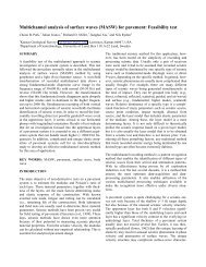
Time-Lapse Seismic Monitoring of Enhanced Oil Recovery CO 2-Flood in a Thin CarbonateReservoir, Hall-Gurney Field, Kansas, U.S.A.Abdelmoneam E. Raef, Richard D. Miller, Alan P. Byrnes, William E. Harrison, and Evan K. FranseenKansas Geological Survey, University of Kansas, 1930 Constant Avenue, Lawrence, Kansas 66047-3726Poster presented at the annual meeting of the American Association of Petroleum GeologistsCalgary, Alberta, Canada, June 22, 2005Original posters were 32” x 44”Content was reformatted to 8½ x 11, only layout modifiedOpen-file Report 2005-24

WHAT ARE THE MOST IMPORTANTFACTORS DETERMINING SELECTION OFA DESTINATION?1. Geographical location and Accessibility2. Cost3. Attractiveness of the destination4. High Quality MICE Infrastructure5. Security6. Unique off-site venues7. Walkability within the destination8. Efficient public transport

Reservoir CharacteristicsReservoir rocks in the C zone are oolitic grainstones that wereoriginally deposited as shallow marine coarse-grained ooidsands concentrated on bathymetric highs on the shelf. Subaerialexposure and meteoric water percolation in the shallow shelfsetting commonly caused ooid dissolution, resulting inoomoldic grainstone textures. The dissolution of ooids alongwith fracturing and crushing (providing connectivity betweenooid molds) resulted in the oomoldic grainstones being theprincipal reservoir rock type (lithofacies). Each of the stackedcyclic deposits within the C zone is characterized by verticallyincreasing porosity and permeability resulting in verticalheterogeneity. Previous study of well log and core data indicatelateral lithofacies changes resulting in lateral heterogeneity.3D Seismic-Reflection ProgramDesign of the seismic survey focused on optimizing the repeatability,acquisition speed, minimized footprint, and azimuthalFigure 4. Acquisition geometry.A variety of surface obstacles affected data qualityand provided challenges during acquisition(Figure 5). Survey repeatability was continuouslychallenged by a variety of logistical aswell as practical problems. A total of nine landownerswere affected by the 2.25 km 2 sourcefootprint while geographically within this smallarea were dozens of pumping units, pastures,cultivated fields, oil field operator storage yards,a major Kansas river, wooded areas, and twocounty roads.Considering the need/necessity for repeatabilityand quiet operations, a high-resolution guidanceand surveying system was customized to provideFigure 5. Pictures from around site.PlattsburgFigure 3. Stratigraphic column for reservoir.and fold coverage, and subsurface resolution. High-foldcoverage encompasses an area about five times largerthan the anticipated size of the pilot study and plannedmovement of CO 2 (Figure 4). This enlarged high-foldfootprint ensured the expected 400 m 2 flood area wasfully sampled. Considering the range of offsets necessaryto capture the ideal reflected seismic energy, a sourcefootprint over 1.5 km 2 and receiver spread of 1 km 2 wasnecessary.A modified brick acquisition pattern was selected tooptimize azimuthal and offset distributions (Figure 4).This configuration is more difficult to acquire, but providesmuch better overall bin-level trace properties. Atotal of 240 receivers were deployed along five lines,each line separated by 200 m and oriented east/west.Source lines were north/south and staggered along linesseparated by 100 m. Source station intervals were 20 m,which yielded 10 m x 10 m bins with 20- to 24-foldsampling redundancy within the high-fold coverage area.source operators with a real-time digital map andlocation logging capabilities (Figure 6). Avoidingequalization techniques during data processingas much as possible was deemed essential,considering the required signal-to-noise levelsand extreme resolution necessary to detect theCO 2 . An overall accuracy of ±5 cm for all x, y,and z source and receiver location measurementswas maintained (Figure 7). Each source locationwas reoccupied during each monitoring surveyFigure 6. GPS on vib. Figure 7. GPS base station at COwithin a tolerance not exceeding 0.5 m.2 injector.Figure 8. Vib track.Data AcquisitionFigure 9. Digital terrain map.Minimal-channel recording equipment and a single vibratory source were thecenterpieces of the acquisition program. Key to this equipment is the low-costseismic monitoring, small footprint, low maintenance, and dependability.A 240-channel distributed seismic recording system from Geometricsprovided 24-bit A/D, short sampling rates (by conventional standards), andextreme flexibility and durability (Figure 10). Each distributed unit wasconnected to a set of 24 geophones via analog seismic cable and to a seismiccontroller by ruggedized Ethernet cables. Data from the ten distributedseismographs (Geodes) were monitored and stored on a specialized landcontroller also from Geometrics (Figure11). The controller was housed in aJohn Deere Gator with a customizedall-weather shelter, allowing operationsin rain or shine from –40 to over+40° C.Figure 12. Compressional wave.Figure 13. Shear wave.Considering the obstacles aroundthis site, night operations wouldnot have been possible withouta pre-mapped route and digitalGPS guidance system, with predesignedroutes updated continuouslythrough GPS feeds insidethe vibrator seismic source (Figure8). The resulting digital terrainmap was incorporated into dataprocessing, providing excellentinformation for datum corrections(Figure 9).Figure 10. Geode seismographs.A single IVI minivib II 14,000-lbseismic vibrator with a prototype highoutputAtlas rotary-style servo valveFigure 11. Recording vehicle.provided the seismic energy for these surveys (Figure 12). In-field rotationof the mass allowed either compressional- or shear-wave data to becollected using the same model vibratory source. Compressional-waveenergy requires the mass to move in a vertical direction, perpendicular tothe ground surface (Figure 12), while for shear-wave energy the motion ofthe mass was parallel to the ground (Figure 13). Five 10-second upsweepsfrom 20 to 250 Hz were recorded at each station for compressional wavesand five 10-second upsweeps from 10 to 80 Hz for shear waves. The firstsweeps were designed to seat the plate only and were not included inprocessed data.

ABBaseline Monitor 1November 2003 January 2004March 2004Monitor 3June 2004 October 2004 March 2005Figure 14. Six surveys, same station.Figure 16. Production well #12 (A), injector #18 (B).Daytime — windyFigure 19. Comparison of wind (20 mph) and calm.Night — calmMonitor 2Monitor 4 Monitor 5Figure 15. Timeline.To date, a total of six 3D surveys have been acquired (Figure 14). Time between surveys has gradually increased fromsix weeks to the current six months between consecutive 3D surveys (Figure 15). Data changes have been observeddue to seasonal weather and soil moisture variability. A total of twelve surveys will be necessary to adequatelycharacterize the efficiency and stability of the CO 2 flood and eventual sequestration.Figure 18. Vehicle noise on seismograms.Vehicle noiseACsurface piston pumppump jackFigure 17. Noise from field activities on seismograms.BDpowerlinewater injection pipelinesAcquisition NoiseTime-lapse seismic data possess reasonablepotential to detect changes inreservoir fluids when all noise—bothsource and environment—is consistentand minimal. Noise associated withwind, vehicles, transmission lines, andfixed pumping facilities (especially inactive oil fields) is a persistent problemwith any seismic survey. In an active oilfield, production wells (Figure 16A),injection wells (Figure 16B), and flowingpipelines produce noise at saturationlevels for most seismic recording systems(Figure 17).Much of the seismic data were acquiredat night to minimize environmental andcultural noise. Vehicle traffic was alsogreatest during the day. Re-shooting stationswhen vehicles were within the survey areawas generally necessary (Figure 18). Windwas a dominant source of noise during daylighthours (Figure 19). With the very weakanomalies, low signal-to-noise, and highresolutionrequirements associated with thesekinds of thin, midcontinent carbonate reservoirs,extraordinary care must be taken withrespect to minimizing noise.Basic Data ProcessingWith the need for horizon-based interpretationsand a high-resolution imageof the CO 2 plume as it expands acrossthe site, the detailed processing flowfocused on reflection-specific enhance-and amplitude analysis. A pro-mentscess referred to as “up-tuned, multiprocessing”was used on paththesedata sets. Instrumental to this type ofprocessing was the modification of thebasic processing flow with each step,cycling back to previous steps toimprove parameters based on downstreamanalysis (Figure 20). Subsequenttime-lapse data sets were incorporatedinto reprocessing of precedingdata sets to ensure all data underwentidentical processing flows. Signalenhancementprocessing focused onnoise removal and improvement ofspectral richness (Figure 21). Datasimilarity between the various monitorsurveys was excellent, with no need forequalization processing to producecomparable preliminary seismicvolumes (Figure 22).• Vertical (temporal) resolution:• Horizontal (spatial) resolution:• Fresnel zone radiusReflecting layerDhFigure 23. Seismic resolution.rh > ¼ λr ≈ √½λDr ≈ ½ V √T 0 /fRBasic Processing FlowUp-tuned multi-path processingMonitor 2Figure 21. Signal enhancement comparison.Figure 22. Similarity of different surveys.0.25λVstackshotgathersTrue Ampl. RecoveryNMOFigure 20. General processing flow.Velocity AnalysisStatics2000 4000Vel. m/s200-400-600-800-Time (ms.)Monitor 2–ProcessedBase Monitor 1ResolutionStacked Vol.Reverse-NMOKey to the effectiveness of seismic-reflectionimaging in many medium and small midcontinentcarbonate reservoirs is resolution, in particularvertical resolution, or the thinnest bed that can bedistinguished from a seismic wavelet (Figure 23).It is generally assumed that one-quarter of awavelength is the thinnest a bed can be and stilldetect top and bottom of the bed. These CMPstacked data possess a dominant frequency ofaround 90 Hz with a usable upper-corner frequencyof about 180 Hz at the depth of interest.These data characteristics equate to a bed-resolutionpotential of around 7 m at 900 m belowground surface. With enhancement processing thedominant frequency is expected to improve toaround 120 Hz to 140 Hz allowing a bed-resolutionpotential of around 4 m.

Considering the importance of spatial tracking of the CO 2 plume as it movesacross this site, horizontal resolution is a key to how effective high-resolutionseismic can be monitoring any EOR program. It is commonly accepted that afraction of the radius of the first Fresnel is approximately equivalent to the sizean object must be to distinguish it as unique on a seismic section. The Fresnelradius for data from this study is about 100 m at 900 m below ground surface(Figure 24). Therefore, any object 100 m or larger can be uniquely detectedwith these seismic data. However, changes in seismic-data character (possiblyindicative of changes in fluid) significantly smaller than the radius of theFresnel zone can be detected.CMP Stacked Section: Seismic CubeIn general, the data quality across this siteis quite good at the L-KC depth of around550 ms (Figure 25). The various seismiccubes can be sliced inline or crosslinerelative to the receiver lines to produce 2Dcross sections. Coherent reflections areprevalent within the time window ofinterest (300 ms to 700 ms).Figure 25. 2D inline time slice of seismic cube.Fresnel radius (m.)3002502001501005000 500 1000 1500 2000 2500 3000Depth (m.)λ=60 m.λ=30 m.λ=10 m.Figure 24. Horizontal resolution at site.Interpretations of time slices tend to support both structural and stratigraphic influences on accumulation andmovement of fluids through the L-KC horizon (Figure 26). Some sense of the lithologic trends potentially influencingwell performance can be gained by comparing and contrasting apparent boundaries or lineaments and changes intexture of specific seismic properties across the site.A prominent feature evident in both data sets is a contrast in properties north and south of an east/west-trending line(A) lying immediately south of well #18 (Figure 26b&d). This trend (A) marks a substantial change in seismiccharacter (both amplitude and frequency) and may indicate the presence of a structural feature or an abrupt change inrock properties. Another lineament (B) follows an amplitude high (red) trend (Figure 26b) and an anomalous group offrequency cells (Figure 26d). This feature, though subtle on both data sets, exhibits a sufficiently high contrast toindicate a marked change in rock properties. A third more subtle northeast/southwest-trending lineament (C) marks atexture change in frequency and an apparent alignment of anomalies in amplitude. Because of the greater sensitivityinstantaneous frequency has to lateral lithologic changes compared to instantaneous amplitude, it seems likely thislineament (C) is related tolithology. It is unlikely thisablineament (C) would havebeen interpreted from amplitudeplots alone.Figure 26. Both amplitude (a) andfrequency attribute plots (c) representingan over 30-m-thick interval of rockthat includes the subsurface interval ofinterest plus around 20 m of rockoverlying and underlying C zone at thissite possess structural and stratigraphicfeatures (b and d) consistent withknown lithology, but at much greaterresolution.cdAACCBBTime-to-Depth CorrelationsA vertical seismic profile (VSP) wasacquired in well #16 and, whencorrelated with well logs, providedan excellent basis for time-to-depthconversions. Data were acquiredwith a 24-channel hydrophonestringer (Figure 27A). Seismicarrivals trailing the first arrivalswere contaminated with tube wave,which hampered full VSP analysisFigure 27B). Using the time-to-depth conversion, it is possible tobulk time-correct the synthetic seismogram for the normalinaccuracy (< 10%) in absolute time resulting from estimatingoverburden velocity.Figure 29. “C” zone horizon on 2D time slice.AFigure 27. VSP survey at well #16 (A), seismogram from borehole (B).Heebner ShPlattsburg LsTime/Depth(sec) (m)Sonic(m/s)BAI Reflectivity KlauderWavelet200-100 HzFigure 28. Synthetic compared to real.Sonic logs from the CO 2 injection well and well #16, combined with a seismic wavelet extracted from real data,were used to generate a conventional synthetic seismogram (Figure 28). A C zone horizon time of 548 ms,established by incorporating the VSP and manual wavelet-correlation techniques, was tracked across all the 3Dseismicvolumes (Figure 29). Considering CO 2 injection interval is only 5 m thick—equating to little more than1 ms—it was imperative to accurately identify the L-KC “C” reflection within a few tenths of a percent.Seismic Modeling and Fluid ReplacementGassmann’s relations can be used to estimate rock-bulk modulus change for thetwo (effective fluid) pore-fluid compositions. For our case the two-fluidcomposition includes the combination of oil-water and miscible CO 2 -oil-water.Average composition effects of reservoir pore-fluid replacement on rockproperty suggests the maximum imageable changes will occur once saturationlevels reach 0.28, at which point a difference of about 10% in seismic amplitudeshould be expected (Figure 30).Attribute AnalysisChange %121086420Synthetic0 0.2 0.4 0.6 0.8 1Effective Fluid Saturation (30%Oil+60%CO2+10Brine)aAverageSeismicTracer=0.68bDelta VelocityDelta DensityDelta AIFigure 30. Fluid replacement model.Lithologic relationships or trends should be observable on lineament-attribute maps of the horizon interpreted asthe L-KC “C” (Figure 31). A strong northeast/southwest series of lineaments are evident across the entirehorizon. The most pronounced ofthese lineaments lies between CO 2 I#1and well #13 and extends across theentire survey area (Figure 32).Another notable lineament extendsfrom about well #13 west betweenwell #12 and injector #18 (Figure32). Also evident is a secondary trendof much smaller and more discontinuouslineaments with a more eastnortheast/west-southwesttrend, especiallypronounced in the northern halfof the survey area.Figure 31. Lineament map “C” horizon.Figure 32. Interpreted lineament map.

4D-Seismic InterpretationCurrently, preliminary processing and interpretationhave been completed on the baseline and first threemonitor surveys. Amplitude-envelope attribute data forthese surveys possess changes in texture generallyconsistent with expectations and CO 2 volumetrics(Figure 40). Arguably, there are a multitude of differentboundaries that could be drawn to define the shape ofthe CO 2 plume, but the shapes suggested match thephysical restraints, based on engineering data and theestimated amplitude response. Focusing on the injectionwell area and continuity of the characteristicsdefining the anomalous area, it is not difficult to identifya notable change in data character and texturelikely associated with the displacement of reservoirfluids with CO 2 .Advancement of the CO 2 from the injector seems tohonor both the lineaments identified on baseline dataand changes in containment pressures. Overlaying theamplitude-envelope attribute map with the lineamentattribute map provides an enhanced view, and thereforeperspective, of the overwhelming variability in thereservoir rocks and the associated consistency andcontrol these features or irregularities have on fluidmovement (Figure 41).Increased northerly movement of the CO 2 , as interpretedon seismic data and inferred from productiondata, after several months of CO 2 injection and oilproduction, stimulated an increase in injection rates atthe water-flood wells (Figure 41B). After severalmonths of increased water-injection rates, the CO 2advancement to the northwest was halted and someregression was observed on seismic data (Figure 41A).Production data did not refute the suggested recedingof the CO 2 front near injection well #10; however,insufficient well coverage exists to provide monitoringat the seismic-resolution levels.Monitor 1Monitor 2Monitor 3Interpretations of time-lapse seismic data are consistentwith and can assist understanding actual fieldresponse data for this pilot study. In a similar fashion,Figure 40. Comparison of amplitude horizon.4D seismic could clearly provide essential input toreservoir simulations necessary for full field EOR-CO 2 floods. Key observation from seismic data include:• accurate indication of solvent “CO 2 ” breakthrough in well #12,• predicted delayed response in well #13,• the interpretation of a permeability barrier between wells #13 and CO 2 I#1, and• consistency with reservoir-simulation prediction of CO 2 movement and volume estimated to havemoved north, outside the pattern.Seismic Results to Enhance Reservoir SimulationsAJanuary2004BMarch2004Simulators are only as “good” as the quality and resolution of the reservoir properties and characteristicsthat make up the models. Initial simulator runs incorporated models based on pre-injection production andwell data alone. These predictions were very dissimilar to actual production measured after commencingEOR-CO 2 injection. All interpretations of seismic data were accomplished without the aid of simulationsupdated with the most current production data; therefore, to a limited extent, the interpretations of CO 2movement on seismic data were accomplished somewhat “blind.” Predictions of breakthrough at #12 andthe delay at #13 were based on seismic data alone after the second monitor survey. General changes in theCO 2 plume and resulting measurements at production wells have been consistent throughout the flood.CJune2004Monitor 1Monitor 2Monitor 3Figure 41. Comparison of amplitude envelope overlineaments.Monitor 4Figure 42. Interpretation of CO 2 and geologic controls.Interpretations of geologic features from seismicdata have provided critical location-specificreservoir properties that appear to strongly influencefluid movement in this production interval.Lineaments identified on seismic sections likely10(based on time-lapse monitoring and production12 CO 216data) play a role in sealing and/or diverting flowthrough the reservoir (Figure 42). By incorporatingthese features using properties consistentwith core data, a more realistic reservoirsimulator results, honoring the production and F1813production and seismic.core properties (Figure 43). Flow models aftersimulator updating (sealing lineaments and preferential permeability manifested byfaster progression of the CO 2 bank) show great improvement in detail and provideexcellent correlation with the material balance (Figure 44).ConclusionsTime-lapse seismic monitoring of EOR-CO 2 canreveal weak anomalies in thin carbonates belowtemporal resolution and can be successful withmoderate cross-equalization and attention toconsistency in acquisition and processing details.Most of all, methods applied here avoid thecomplications associated with inversion-basedattributes and extensive cross-equalizationtechniques.Shortness of turnaround time of time-lapseseismic monitoring in the Hall-Gurney fieldprovided timely support for reservoir-simulationadjustments and flood-management requirementsacross this very short-lived pilot study.Spatial textural, rather than spatially sustainablemagnitude, time-lapse anomalies were observedand should be expected for thin, shallow carbonatereservoirs. Non-inversion, direct seismicattributes proved both accurate and robust formonitoring the development of this EOR-CO 2flood.Distribution and geometries associated withsimilarity-seismic facies and seismic-lineamentpatterns are suggestive of a complex ooid shoaldepositional motif, consistent with ooliticlithofacies being the known reservoir in thisfield. Oolitic facies are imaged on these seismicdata at a resolution significantly greater thanpreviously documented.Acknowledgmentsigure 43. Variability of permeability based on101210121012CO 218CO 21818Monitor 1Monitor 2Monitor 3Figure 44. Simulations for seismic surveytimes.Support for this project was provided by the National EnergyTechnology Laboratory at the U.S. Department of Energyunder grant DE-FC26-03NT15414.CO 2131313161616