State-Space Modelling of Dynamic Systems Using Hankel ... - ijcset

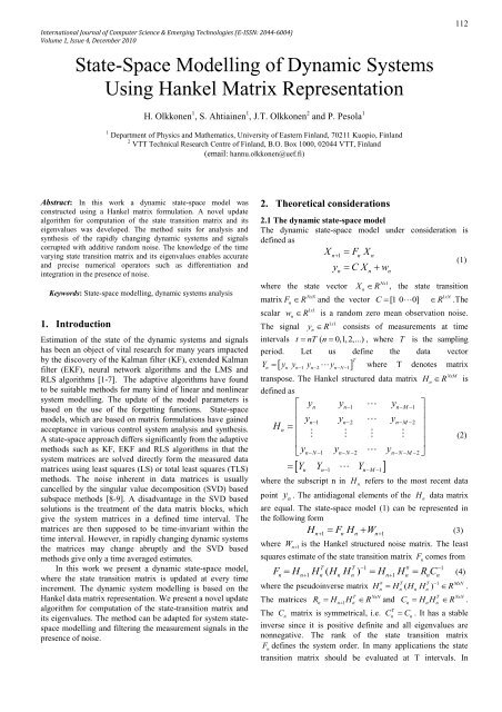
International Journal of Computer Science & Emerging Technologies (E-ISSN: 2044-6004)Volume 1, Issue 4, December 2010State-Space Modelling of Dynamic SystemsUsing Hankel Matrix Representation112H. Olkkonen 1 , S. Ahtiainen 1 , J.T. Olkkonen 2 and P. Pesola 11Department of Physics and Mathematics, University of Eastern Finland, 70211 Kuopio, Finland2VTT Technical Research Centre of Finland, B.O. Box 1000, 02044 VTT, Finland(email: hannu.olkkonen@uef.fi)Abstract: In this work a dynamic state-space model wasconstructed using a Hankel matrix formulation. A novel updatealgorithm for computation of the state transition matrix and itseigenvalues was developed. The method suits for analysis andsynthesis of the rapidly changing dynamic systems and signalscorrupted with additive random noise. The knowledge of the timevarying state transition matrix and its eigenvalues enables accurateand precise numerical operators such as differentiation andintegration in the presence of noise.Keywords: State-space modelling, dynamic systems analysis1. IntroductionEstimation of the state of the dynamic systems and signalshas been an object of vital research for many years impactedby the discovery of the Kalman filter (KF), extended Kalmanfilter (EKF), neural network algorithms and the LMS andRLS algorithms [1-7]. The adaptive algorithms have foundto be suitable methods for many kind of linear and nonlinearsystem modelling. The update of the model parameters isbased on the use of the forgetting functions. State-spacemodels, which are based on matrix formulations have gainedacceptance in various control system analysis and synthesis.A state-space approach differs significantly from the adaptivemethods such as KF, EKF and RLS algorithms in that thesystem matrices are solved directly form the measured datamatrices using least squares (LS) or total least squares (TLS)methods. The noise inherent in data matrices is usuallycancelled by the singular value decomposition (SVD) basedsubspace methods [8-9]. A disadvantage in the SVD basedsolutions is the treatment of the data matrix blocks, whichgive the system matrices in a defined time interval. Thematrices are then supposed to be time-invariant within thetime interval. However, in rapidly changing dynamic systemsthe matrices may change abruptly and the SVD basedmethods give only a time averaged estimates.In this work we present a dynamic state-space model,where the state transition matrix is updated at every timeincrement. The dynamic system modelling is based on theHankel data matrix representation. We present a novel updatealgorithm for computation of the state-transition matrix andits eigenvalues. The method can be adapted for system statespacemodelling and filtering the measurement signals in thepresence of noise.2. Theoretical considerations2.1 The dynamic state-space modelThe dynamic state-space model under consideration isdefined aswhere the state vectormatrix FscalarThe signalX n1Fn Xny C X wn n nXn RNx1(1), the state transition1xN R.TheNxNn R and the vector C [1 0 0]11 xwn R is a random zero mean observation noise.yn11 x R consists of measurements at timeintervals t nT ( n 0,1,2,...) , where T is the samplingperiod. Let us define the data vectorn n n1 n2 nN1TY y y y y where T denotes matrixtranspose. The Hankel structured data matrixdefined asHn y y y y y yy y y Y Y Yn n1 nM1n1 n2 nM2nN 1 nN 2 nN M2n n1 nM1HnNxM R iswhere the subscript n in Hnrefers to the most recent datapoint yn. The antidiagonal elements of the Hndata matrixare equal. The state-space model (1) can be represented inthe following formH F H W(3)n1 n n n1where Wn 1squares estimate of the state transition matrix(2)is the Hankel structured noise matrix. The leastFncomes fromF H H ( H H ) H H R C (4)T T 1 # 1n n1 n n n n1n n nwhere the pseudoinverse matrixH H ( H H ) R .# T T 1MxNn n n nT NxNT NxNThe matrices Rn Hn1HnRand Cn HnHn R .TThe Cnmatrix is symmetrical, i.e. Cn Cn. It has a stableinverse since it is positive definite and all eigenvalues arenonnegative. The rank of the state transition matrixFndefines the system order. In many applications the statetransition matrix should be evaluated at T intervals. In

International Journal of Computer Science & Emerging Technologies (E-ISSN: 2044-6004)Volume 1, Issue 4, December 2010113complex dynamic systems the dimension of the statetransition matrix is high and the computation of thepseudoinverse matrix H would be an overwhelming task. In#nthis work we show that with a special partitioning the RnandCnmatrices into submatrices the computational load isdrastically diminished.2.2 Computation of the state transition matrix FnThe data matrix Hnis partitioned aswhere the matrixHDnnDn d n ( N 1) xM R and the vectorThe data matrix Hn 1is partitioned asHn1d Dn1ndn(5)1xM R .1xMwhere the vector d n1R and the matrix Dnis identical tothat in (5). Now we haveT TDn T TDn Dn DndnCn Dn dn T Td n dnDn dndnA bnTnbcnnwhere the matrix( N 1) x1bn R and the scalarthe inverse matrix iscnA R (6)(7)( N 1) x( N 1)n , the vector R11 x. The analytic solution of1 1T1 An bnAn snmnmn snmnn T Tbn cn snmn sn C where the vector(8)m A b Rand the scalar1 ( N1) x1n n nT 1 1x1n (nn n) . The inverse matrix has the sames c b m Rblock dimensions as thehaveCnmatrix. Correspondingly, weT dn1 T TRn Hn1Hn Dn dnD n where the vectorTTdn 1Dn dn 1d en ng n TT D AnDn Dndnnb n1 xN ( 1) R and the scalar Rengn11 x(9). Thematrix Anand the vector bnare identical to in (7). Now weobtain the state transition matrix asF R C1n n nwhich finally yields1Ten gnAn snmnmn snmn TAn b n snmn snhnFn Ikn (10)where the scalar kn gnsn snenmnand the vector1 T( N 1) x( N 1)h e A k m . The identity matrix IR and then n n n n( N 1) x1R zero vector .2.3 Updating the state transition matrix FnThe updated matrix Cn 1is partitioned into the four subblocksTTdn1 T Tdn 1dn 1dn 1D nCn1 dn 1Dn T TD n Dnd n1Dn Dnp en1TnenA n(11)where pn 1is a scalar. The essential observation is that Cn 1contains a submatrix A n, which is the same as in partitioningthe Cnmatrix (7). The vector enequals to that in (9). Theanalytic matrix inversion givesC1n1where the vector1pn1en TenA n rn 1 rn 1qn T 1Trn 1qn An rn 1qn q n q(12) e A and the scalar1n n n11( Tnn1 n n) . We may note that the vectornr p q e q ispreviously computed as a first term in vector hnin (10).1Finally, the computed C n 1matrix is represented in therepartitioned form (7)C1n1A bwhere the vectorbn1 n1Tn1 cn11A s m m s m Tn1 zn1 Tzn1w n11n1 n1 n1 Tn1 n1 n1Tsn 1mn1 sn1(13)m A b and the scalar1n1 n1 n11s1( ncn 1bn 1mn)( N 1) x( N 1). The matrixT n 1R ( N 1) x1z n 1R 11 xwn1 R are picked up1C n 1(12). By comparingvectorfrom the computed inverse matrixthe block matrices we obtain the solution for the vector1and the inverse block matrix A as mn 1n 11n1 n1 n1m w zNow we get the updated Rn 1Rn1A T m z1Tn1 n1 n1 n1e Amatrixgn1 n1bn1 n1(14)(15)

International Journal of Computer Science & Emerging Technologies (E-ISSN: 2044-6004)Volume 1, Issue 4, December 2010114where the vectoreRg R .comes 1 xN ( 1)and the scalar 11 xn1n 1Finally, the uptake of the state transition matrix Fn 1fromF R C1n1 n1 n11Ten1 gn 1An 1 sn 1mn1mn 1 sn 1m n1 TAn 1b n1 sn 1mn1 sn1 hn1 kn1 I k g s s e m(16)where the scalarn1 n1 n1 n1 n1 n1and the vector1Th e A k m . An interesting feature is that then1 n1 n1 n1 n1vector bn 1needs not to be known in the uptake process (16).2.4 Fast uptake of the RnmatrixThe uptake process (16) needs the computation of the vectorTTen 1 dn2Dn1and the scalar gn 1 dn2dn1, if partitioning(5) is used. This would require one vector-matrix and onevector-vector multiplication. Fast uptake of the Rnmatrix isobtained if we adapt the partitioning (2) for the data matrixH Y Y Y(17)n n n1 nM1Now we haveT T TR [ Y Y Y Y Y Y ] (18)n n1 n n n1 nM nM1and the uptake of theThe uptake of theR matrix is yielded asnR R Y Y Y Y(19)TTn1 n n2 n1 nM nM1R matrix needs only two vector-vectornmultiplications and the vector en 1and the scalar gn 1aresimply picked up from the Rn 1matrix (19).2.5 Computational complexityThe uptake of the state transition matrix requires the1computation of the matrix inverse C n 1(12), which needs onevector-vector multiplication. The uptake of the vector1m and the inverse block matrix (14) needs onen 1A n1vector-vector multiplication. Finally, the uptake of the scalarkn 1and the vector hn 1in (16) requires one vector-matrixand three vector-vector multiplications. Thus thecomputational complexity of the algorithm is2O( n ) 5 O( n).3. Applications of the method3.1 Computation of the eigenvalues of the state transitionmatrixThe Hankel data matrix representation (3,5) of the dynamicstate-space model leads to a companion matrix structure ofthe state transition matrix F (10) , which involves only thenvector hnand the scalar kn. An important advantage of thecompanion matrix structure is that the eigenvalues1, 2,..., Nof the state transition matrix can be directlycomputed as the roots of the polynomial having coefficients[1 - h n- k n]. The eigenvalues of the state transition matrixgive important knowledge of the order and the stability of thesystem and its dynamic behaviour. The eigenvalues also aidin selection of the model order. The occurrence of very smalleigenvalues indicates that the system order is smaller that themodel order, which leads to overmodelling. When the modelorder equals the system order, the scalar coefficient knattainsa value kn 1.3.2 Signal prediction and state-space filteringThe knowledge of the state transition matrix F enables theprediction of the measurement signal ynasH F H yˆ C F H(20)n1 n n n1n n1xNwhere C [1 0 0] R . Using the Hankel data matrixrepresentation we may define the prediction data matrix asHˆn yˆ yˆ yˆyˆ yˆ yˆ yˆ yˆ yˆ Hˆ F Hˆn n1 nM1n1 n2 nM2nN 1 nN 2 nN M2n1n nn(21)The state-space filtered signal yˆncan be obtained as a meanof the antidiagonal elements. In the following we describeseveral matrix operators based on the state transition matrix.In all computations the filtered data matrix (21) is applied.3.3 Numerical signal processingThe knowledge of the state transition matrix F nenables thenumerical signal processing of the state-space filtered signal.In the following we develop matrix operators based on thestate transition matrix for numerical interpolation,differentiation and integration of the measurement signal.The state transition matrix can be presented in the1eigenvalue decomposited form F U D U , whereNxNDnR diag( 1 2N)andUwe have a resultˆ ˆ 1H ˆn1 Fn Hn UnDnU nHnˆ 1ˆ ˆnn n n nn nH U D U H F Hn n n nNxNn R . Based on (21)(22)where the time-shift [0, T]. Now we may define theinterpolating time-shift operator Sn, NxNR Hˆ S Hˆ S F (23)n n, n n, nNext, we may define the differentiation operatorasDn Rd H ˆ ˆ ˆ D n ˆn Dn Hn Hn1 e Hn(24)dtDue to (20) we haveDF e n D log m( F )(25)n n nwhere log m( ) denotes matrix logarithm.NxNFurther, by defining the integral operator In R asˆ ˆ Hndt InHn(26)NxN

International Journal of Computer Science & Emerging Technologies (E-ISSN: 2044-6004)Volume 1, Issue 4, December 2010115Since the differentiation and integral operator are inverseoperators11ˆ ˆ log ( ) ˆn n n n n nI H D H m F H In log m( F )n1and the definite integral is yielded asnT( nd ) THˆdtlog ( ) log ( ) n1 1m F m F Hˆn nd n(27)(28)The interpolating, differentiation and integral operators arecommutative, i.e. SnDn Dn Snand SnIn InSn. Thecomputation of the second, third etc. derivatives and integralsof the signals are also possible using the matrix operators,e.g. the second derivative operator is obtained2as 2Dn log m( F )n. It should be pointed out that applied tothe state-space filtered signals the numerical operators areanalytic, i.e. they produce results with machine precision.4. DiscussionThe distinct difference between the present algorithm and theSVD based methods is that the present algorithm updates thestate transition matrix Fnat every time interval, while theSVD based algorithms [8-9] compute the state transitionmatrix in data blocks. Our algorithm is more feasible in theanalysis of the fastly changing dynamic systems andespecially for real-time applications, where the eigenvaluesof the state transition matrix give actual information on thesystem functioning.A key idea in this work is the repartitioning scheme (13),which yields the uptake of the vector mn 1and the inverse1block matrix (14) and then the uptake of the stateA n 1transition matrix Fn 1(16). The companion matrix structureof the matrix F nenables the computation of the eigenvaluesof the state transition matrix via the roots of the polynomial[1 - h n- k n]. This procedure is much faster than the directeigenvalue decomposition of the Fnmatrix. The knowledgeof the eigenvalues yields a plenty of numerical signalprocessing tools, such as interpolation, differentiation andintegration operators (21,22,26), which compete with theconventional B-spline signal processing algorithms [10-12].References[1] F. Daum, Nonlinear filters: Beyond the Kalman Filter,IEEE A&E Systems Magazine, vol. 20, pp. 57-69, Aug.2005.[2] A. Moghaddamjoo and R. Lynn Kirlin, “Robust adaptiveKalman filtering with unknown inputs,” IEEE Trans.Acoustics, Speech and Signal Process. vol. 37, No. 8,pp. 1166-1175, Aug. 1989.[3] J. L. Maryak, J.C. Spall and B.D. Heydon, “Use of theKalman filter for interference in state-space models withunknown noise distributions,” IEEE Trans. Autom.Control, vol, 49, No. 1, pp. 87-90, Sep. 2005.[4] R. Diversi, R. Guidorzi and U. Soverini, “Kalmanfiltering in extended noise environments,” IEEE Trans.Autom. Control, vol. 50, No. 9, pp. 1396-1402, Sep.2005[5] D.-J. Jwo and S.-H. Wang, Adaptive fuzzy strongtracking extended Kalman Filtering for GPS navigation,IEEE Sensors Journal, vol. 7, no. 5, pp. 778-789, May2007.[6] S. Attallah, The wavelet transform-domain LMSadaptive filter with partial subband-coefficient updating,IEEE Trans. Circuits and Systems II, vol. 53, no. 1, pp.8-12, Jan. 2006[7] H. Olkkonen, P. Pesola, A. Valjakka and L. Tuomisto,“Gain optimized cosine transform domain LMSalgorithm for adaptive filtering of EEG,” Comput. Biol.Med, vol, 29, pp. 129-136, 1999.[8] S. Park, T.K. Sarkar and Y. Hua, A singular valuedecomposition-based method for solving a deterministicadaptive problem, Digital Signal processing 9, 57-63,1999.[9] T.J. Willink, “Efficient adaptive SVD algorithm forMIMO applications,” IEEE Trans. Signal Process., vol.56, no. 2, pp.615-622, Feb. 2008.[10] M. Unser, A. Aldroubi and M. Eden, “B-spline signalprocessing. I. Theory,” IEEE Trans. Signal Process.,vol. 41, no. 2, pp. 821-833, Feb. 1993.[11] M. Unser, A. Aldroubi and M. Eden, “B-spline signalprocessing. II. Efficiency design and applications,” IEEETrans. Signal Process., vol. 41, No. 2, pp. 834-848,Feb. 1993.[12] J.T. Olkkonen and H. Olkkonen, “Fractional time-shiftB-spline filter,” IEEE Signal Process. Letters, vol. 14,No. 10, pp. 688-691, Oct. 2007.