Lagrangian Particle Tracking on a GPU. pdfauthor - User Websites ...

<strong>Lagrangian</strong> <strong>Particle</strong> <strong>Tracking</strong> on a GPUAuthorNils BrünggelAdvisorsProf. Jörg HofstetterProf. Dr. Josef BürglerJuly 15, 2011

Contents1 Introduction 11.1 Motivation . . . . . . . . . . . . . . . . . . . . . . . . . . . . . . . . . . . . . . . . 11.2 Project Goal . . . . . . . . . . . . . . . . . . . . . . . . . . . . . . . . . . . . . . . 12 OpenFOAM 22.1 Introduction . . . . . . . . . . . . . . . . . . . . . . . . . . . . . . . . . . . . . . . . 22.2 Mesh Representation . . . . . . . . . . . . . . . . . . . . . . . . . . . . . . . . . . . 22.3 The <strong>Lagrangian</strong> Framework . . . . . . . . . . . . . . . . . . . . . . . . . . . . . . . 22.4 Parallelization and Support for GPUs . . . . . . . . . . . . . . . . . . . . . . . . . 53 The <strong>Particle</strong> <strong>Tracking</strong> Algorithm 63.1 Basic <strong>Particle</strong> <strong>Tracking</strong> Algorithm . . . . . . . . . . . . . . . . . . . . . . . . . . . 63.2 Modified <strong>Tracking</strong> Algorithm . . . . . . . . . . . . . . . . . . . . . . . . . . . . . . 73.3 Implementation in OpenFOAM (solid<strong>Particle</strong> Library) . . . . . . . . . . . . . . . . 84 GPU Computing 94.1 Introduction . . . . . . . . . . . . . . . . . . . . . . . . . . . . . . . . . . . . . . . . 94.2 Architecture of Modern GPUs . . . . . . . . . . . . . . . . . . . . . . . . . . . . . . 94.3 CUDA . . . . . . . . . . . . . . . . . . . . . . . . . . . . . . . . . . . . . . . . . . . 105 Software Development 125.1 Software Design . . . . . . . . . . . . . . . . . . . . . . . . . . . . . . . . . . . . . . 125.2 Complete <strong>Particle</strong> Engine . . . . . . . . . . . . . . . . . . . . . . . . . . . . . . . . 145.3 Data Reduction . . . . . . . . . . . . . . . . . . . . . . . . . . . . . . . . . . . . . . 165.4 Tools and Validation . . . . . . . . . . . . . . . . . . . . . . . . . . . . . . . . . . . 176 Test Cases and Results 186.1 Tunnel . . . . . . . . . . . . . . . . . . . . . . . . . . . . . . . . . . . . . . . . . . . 186.2 Torus . . . . . . . . . . . . . . . . . . . . . . . . . . . . . . . . . . . . . . . . . . . 186.3 Measurements . . . . . . . . . . . . . . . . . . . . . . . . . . . . . . . . . . . . . . . 196.4 Performance Analysis of Computational Kernels . . . . . . . . . . . . . . . . . . . 216.5 Memory Requirements . . . . . . . . . . . . . . . . . . . . . . . . . . . . . . . . . . 227 Conclusion and Future Work 248 Summaries of Related Works 258.1 Nvidia’s <strong>Particle</strong>s Demo . . . . . . . . . . . . . . . . . . . . . . . . . . . . . . . . . 258.2 The <strong>Lagrangian</strong> <strong>Particle</strong>s in the EM Driven Turbulent Flow with Fine Mesh . . . . 258.3 Complex Chemistry Modeling of Diesel Spray Combustion . . . . . . . . . . . . . . 258.4 Porting Large Fortran Codebases to GPUs . . . . . . . . . . . . . . . . . . . . . . . 269 Appendix 279.1 Assertions on the GPU . . . . . . . . . . . . . . . . . . . . . . . . . . . . . . . . . . 279.2 Curriculum Vitae . . . . . . . . . . . . . . . . . . . . . . . . . . . . . . . . . . . . . 289.3 Project Definition . . . . . . . . . . . . . . . . . . . . . . . . . . . . . . . . . . . . . 28I

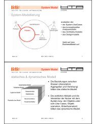
List of Figures1 Class diagram outlining the solid<strong>Particle</strong> library. . . . . . . . . . . . . . . . . . . . 32 Illustration of circular dependencies in OpenFOAM using templates and inheritance. 33 Example situation in two dimensions illustrates the particle tracking algorithm. . . 64 Two dimensional illustration of a particle trajectory through multiple cells. . . . . 85 Nvidia’s Fermi architecture, taken from [25]. . . . . . . . . . . . . . . . . . . . . . . 106 Cell centres arranged in memory. . . . . . . . . . . . . . . . . . . . . . . . . . . . . 127 Mesh data layout in memory. . . . . . . . . . . . . . . . . . . . . . . . . . . . . . . 128 Owner and neighbour data of the particle tunnel case. . . . . . . . . . . . . . . . . 139 Simplified class diagram of the GPU tracking library. . . . . . . . . . . . . . . . . . 1410 Complete particle tracking sequence. . . . . . . . . . . . . . . . . . . . . . . . . . . 1511 Reducing the particle labels array to those which sill need tracking. . . . . . . . . . 1612 Width plot of the GPU time spent for calculating lambdas. The CPU is used fordata reduction. . . . . . . . . . . . . . . . . . . . . . . . . . . . . . . . . . . . . . . 1613 <strong>Particle</strong> tunnel with randomly distributed particles. . . . . . . . . . . . . . . . . . 1814 A torus defined by surface revolution of a circle. . . . . . . . . . . . . . . . . . . . 1815 A tetrahedral mesh generated in a torus. . . . . . . . . . . . . . . . . . . . . . . . . 1916 Plot showing the execution time for a growing number of particles. . . . . . . . . . 2017 Width plot showing the time of kernel functions and memcpy operations. . . . . . 2118 Width plot showing the actual time spent on the GPU. . . . . . . . . . . . . . . . 21II

Erklärung der SelbstständigkeitHiermit erkläre ich, dass ich die vorliegende Arbeit selbstständig angefertigt und keine anderen alsdie angegebenen Hilfsmittel verwendet habe. Sämtliche verwendeten Textausschnitte, Zitate oderInhalte anderer Verfasser wurden ausdrücklich als solche gekennzeichnet.Horw, 15. Juli 2011Nils Brünggel

AcknowledgmentsI would like to thank the many people who helped me completing this thesis. Especially my advisorJosef Bürgler who took the time to discuss the many problems I ran into during this work andhelped me to develop solutions for it. Brahim Aakti who thought me many things about fluiddynamics that I never learned as a computer science student. Thomas Koller who helped mebetter understanding C++ and reviewed my software design. Luca Mangani for discussing theimplementation in OpenFOAM. And all the people who read this thesis (or parts of it) and gavefeedback: Antoine Hauck, Kym Brünggel, Marcel Brünggel and David Roos Launchbury.IV

AbstractIn addition to the most common numerical method, the finite volume method, particlesare often used in complex fluid simulations. For example when simulating combustion in aDiesel engine the droplets are modeled as particles while the fluid is calculated in a discretemesh. The two phases are called Eulerian and <strong>Lagrangian</strong>. While the <strong>Lagrangian</strong> phase doesnot need a mesh itself, coupling it with the Eulerian phase requires to know, for each timestep, in which cell the particles reside. If unstructured meshes are used it is not trivial tofind a particles occupancy cell, given its position. To do so a sophisticated particle trackingalgorithm was developed.When using particles it is usually desirable to use a large number of particles, because thisleads to better results. The aim of this project was to track particles more efficiently. Becausethe particle tracking algorithm tracks each particle individually it is suitable for massivelyparallel computing. A graphics processing unit (GPU) was used which can run thousands ofthreads concurrently.Using an existing computational fluid dynamics (CFD) package, OpenFOAM, a simplesolver was developed in which particles are dragged by a given velocity field through themesh. This work involved converting the mesh and particle data into structures suitable forparallel processing as well as porting the algorithm to the GPU. Testing and validating thecode was the biggest part: Because of the lack of object oriented constructs for the code onthe GPU, the data was stored in simple arrays making it necessary to calculate array indicesin the program. This lead to rather error prone code. To ensure correctness the intermediateresults of the sequential implementation were extracted and compared to the results of thenew parallel implementation. Finally a switch was added to the solver which causes a meshsearch after each time-step: For each particle a mesh search is executed for its end positionrevealing the actual occupancy cell. This is then compared with the new occupancy calculatedby the newly-developed particle tracking algorithm. If it is turned on, one can ensure thatoccupancy cells of all particles are correct. This, of course, makes the solver extremely slow.Comparing the computation time for the tracking algorithm revealed a huge speedup. TheGPU implementation is around 30 times faster compared to the sequential implementationin OpenFOAM. Because it is necessary to copy all the data over a slow bus to the GPU thepractical execution time is slower, but still much faster than the sequential implementation.V

1 Introduction1.1 MotivationIn computational fluid dynamics (CFD) the finite volume method (FVM) is most commonly usedto solve the partial differential equations (PDE) which describe the fluid flow. In order to discretizethe simulation domain a mesh is constructed which covers the whole domain. The equations arethen evaluated at the centroid of each cell and the results, such as velocity, pressure, temperature,etc are stored for each cell. In addition to the FVM some parts of a simulation may be modeled asparticles such as Diesel droplets in an engine. [24] The gaseous phase, represented in the mesh,is called Eulerian, while the liquid phase, represented by particles, is called <strong>Lagrangian</strong>. Thoseare different ways of looking at the flow field. In the <strong>Lagrangian</strong> view the observer follows anindividual particle as it moves through space and time. This can be visualized as sitting in a boatand drifting down a river. The Eulerian specification of the flow field is a way of looking at fluidmotion that focuses on specific locations in space through which the fluid flows as time passes.This can be visualized by sitting on the bank of a river and watching the water pass the fixedlocation. [8] There are different levels of coupling between these two phases: If the <strong>Lagrangian</strong>particles are just dragged by the Eulerian phase one refers to this as a one-way coupling. If the<strong>Lagrangian</strong> particles also influence the Eulerian phase it is called a two-way coupling. The meshplays an important role when the two phases are coupled: The Eulerian equations are evaluatedat the centroid of every cell. The <strong>Lagrangian</strong> particles do not need a mesh themselves, but thecoupling requires it to know in which cell a particle resides so that the coupling terms can beappended to the Eulerian phase. More specifically we need to know for every time step throughwhich cells the particle travels and how much time it spends in each cell.It is distinguished between structured and unstructured meshes. Structured refers to the wayhow the mesh data is stored in memory: A direct mapping between the connections in the meshand the addresses of the data exists. This structure restricts the shape of the cells in the meshto hexahedra. Unstructured meshes on the other hand allow cells with any number of faces, thismakes them more flexible but also increases the amount of work a program has to do, for exampleto access a cell next to a given cell. Structured meshes can be transformed into a uniform cartesiangrid. [4] It is therefore trivial to find the cell in which a particle resides, given its position. Inan unstructured mesh this is no longer possible and requires a sophisticated algorithm which isexplained in section 3. OpenFOAM comes with support for unstructured meshes because thismakes it simpler to automatically mesh complex geometries from a CAD system and it simplifiesthe import of meshes from different meshing tools. [19]1.2 Project Goal<strong>Particle</strong> tracking requires the execution of simple vector calculations for a large number of particles.This can be achieved more efficiently by using a massively parallel processor such as a GPU(see section 4). Based on the existing OpenFOAM code the goal is to develop a solver whichmoves particles using the velocity field from the mesh. The solver will use the GPU to executethe computations required for the particle tracking algorithm in a massively parallel way, whichwill lead to great speedup compared to the already existing single-threaded implementation inOpenFOAM. The original project definition can be found in the appendix, section 9.3.1

2 OpenFOAM2.1 IntroductionOpenFOAM is an open source framework for computational fluid dynamics. It is entirely writtenin C++ and licensed under the GNU General Public License (GPL). OpenFOAM comes with basicmeshing tools, various solvers and utilities to import meshes and export data for post processing.As opposed to many commercial packages the OpenFoam tools do not provide a graphical userinterface. Instead the user has to edit configuration files within an OpenFOAM case and then runthe solver in a UNIX-like fashion on the command line. One of the strengths of OpenFOAM isthat custom solvers can be written or modified quickly because of its modular design and the usageof advanced C++ features.2.2 Mesh RepresentationOpenFOAM supports unstructured polyhedral meshes with any number of faces. The mesh isdescribed in the official Users Guide [6] (chapter 5), the Programmers Guide [5] (chapter 2.3) aswell as in Jasak’s PhD thesis [18] (chapter 3.2). Here I will recall a short summary. OpenFOAMstores the mesh in the following files 1 , which are generated by mesh utilities such as blockMesh.• points Contains a list of coordinates of vertices. OpenFOAM implicitly indexes the pointsstarting from 0 up to the number of points minus one.• faces Contains a list of faces. The point indices defined in the points file are used toreference the vertices. It is distinguished between internal faces and boundary faces: Internalfaces are between two cells and always have an owner and a neighbour cell assigned, whileboundary faces lie on the boundary of the computational domain and just have an owner cellassigned (see below). Further a face normal is defined, so that it points outside of the ownercell. In case the face is a boundary face, the normal points outside of the computationaldomain.The order of the vertices of a face is defined such that, if the normal vector points towardsthe viewer, the vertices are arranged in an anti-clockwise path. The faces are also implicitlyindexed, starting with 0 for the first face.It is common that the faces inside the simulation domain, called inner faces have a lower facelabel than those on the boundary, called boundary faces. OpenFOAM lets the user definevarious boundary conditions by referring a set of boundary faces.• owner Each face is assigned an owner cell, in case of an internal face this is the cell withthe lower label of the two cells adjacent to the face. The face normal can also be defined aspointing from the cell with the lower label to the cell with the higher label.• neighbour Internal faces also have a neighbour cell. Since an internal face is always betweentwo cells, the cell not being the owner is the neighbour cell. (Which is the cell with the higherlabel.) Faces lying on the boundary have no neighbour cell and are omitted in the neighbourlist. Since some faces always lie on the boundary, this list has less items then the owner list.• boundary The boundary file contains a list of patches which refer to a set of boundary faces.2.3 The <strong>Lagrangian</strong> FrameworkOpenFOAM includes a <strong>Lagrangian</strong> framework which was originally developed to simulate Dieseldroplets [24]. The simplest <strong>Lagrangian</strong> library allows the simulation of solid particles which aremoved by the Eulerian field. The work carried out here is based on the solidPartilce library.1 Located in constant/polyMesh in an OpenFoam case directory.2

<strong>Particle</strong>vector position_label celli_label facei_scalar stepFraction_+ readFields()+ writeFields()+ write()+ position()+ cell()+ trackToFace()<strong>Particle</strong>TypefriendIDLListIntrusively doubly-linked list.CloudA collection of particles.+ void move(<strong>Tracking</strong>Data& td)solid<strong>Particle</strong>Cloudfriend A collection of particles.<strong>Particle</strong>TypefriendIOPositionHelper IO class to read and write particlepositions+ virtual void readData(Cloud& c,bool checkClass)+ virtual bool write() const+ virtual bool writeData(Ostream& os) const<strong>Particle</strong>Typesolid<strong>Particle</strong>Simple solid spherical particle classwith one-way coupling with thecontinuous phase.- scalar d_- vector U_+ bool move(trackData&);+ void hitWallPatch (const wallPolyPatch&,int&);void move(const dimensionedVector& g)Figure 1: Class diagram outlining the solid<strong>Particle</strong> library.Figure 1 shows the most important classes belonging to the solid<strong>Particle</strong> library. Note that,for the sake of simplicity not all class members are shown. The particles are stored in a doublylinked list. The particle tracking algorithm is implemented in a flexible way: The most basicfunctionality is in the <strong>Particle</strong> class via the trackToFace() function. Functionality specific to acertain particle type, such as the drag model, is implemented in the solid<strong>Particle</strong> class. Thesolid<strong>Particle</strong> class provides the move() method which is called from the solid<strong>Particle</strong>Cloudclass for every particle. Using the specific drag model the destination for a particle is estimated,trackToFace() is then called with the before calculated destination.Usage of curiously recurring template patterns When looking at the classes of the solid<strong>Particle</strong>library a remarkable circular dependency between derived classes can be found. For example theclasses <strong>Particle</strong> and solid<strong>Particle</strong> in the <strong>Lagrangian</strong> framework. solid<strong>Particle</strong> is derivedfrom the <strong>Particle</strong> class template which takes the type of the derived class as template argument.<strong>Particle</strong>solid<strong>Particle</strong>Figure 2: Illustration of circular dependencies in OpenFOAM using templates and inheritance.The dependency goes in one direction via inheritance and in the other direction via templates.This pattern was named ”Curiously Recurring Template Pattern (CRTP)” by James Coplien3

in 1995 [14]. It can be used to implement static polymorphism without the need to use virtualfunctions, as illustrated in the example below.1 # include 23 template 4 struct A {56 void doSomething () {7 static_cast < DerivedType & >(* this ). doSomethingElse ();8 }9 };1011 struct B: public A {1213 void doSomethingElse () {1415 printf (" Hello ␣ from ␣B!\n");16 }17 };1819 struct C: public A {2021 void doSomethingElse () {2223 printf (" Hello ␣ from ␣C!\n");24 }25 };262728 int main () {2930 B b;31 b. doSomething ();32 C c;33 c. doSomething ();3435 return 0;36 }3738 // Output3940 Hello from B!41 Hello from C!As mentioned before this idiom is used in the <strong>Lagrangian</strong> classes 2 . The <strong>Particle</strong> class isdeclared as follows:1 template < class <strong>Particle</strong>Type >2 class <strong>Particle</strong> : public IDLList < <strong>Particle</strong>Type >:: link {3 // ..4 };And the solid<strong>Particle</strong> class as follows:1 class solid<strong>Particle</strong> : public <strong>Particle</strong> < solid<strong>Particle</strong> > {2 // ..3 };2 This can be found in the OpenFOAM source tree in the directory src/lagrangian4

The particle class can now call members which are to be defined in their derived classes using astatic cast on the this-pointer.1 static_cast < <strong>Particle</strong>Type & >(* this )Using a reference to the derived type it can be checked weather the particle is of a special typeas done on line 299 from the file <strong>Particle</strong>.C:1 // ..2 else if ( static_cast < <strong>Particle</strong>Type & >(* this ). softImpact ())3 {45 // ..This is just one example in which this idiom is used and there are many more within the codeof OpenFOAM.2.4 Parallelization and Support for GPUsThe OpenFOAM code is mostly sequential C++ code. Larger simulations can be decomposed intovarious domains and multiple instances of a solver can be launched which communicate using themessage passing interface (MPI) [10]. While OpenFOAM currently does not support fine grainedparallelism, it has recently been shown that OpenFOAM could benefit a hybrid parallelizationmodel where OpenMP is used in addition to MPI for the fine grained parallelization on each host[20].There is officially no support for GPU computing in OpenFOAM, however various third-partysolutions exist. The [21] SpeedIT tools make it possible to use OpenFOAM with CUBLAS,Nvidia’s implementation of BLAS (Basic Linear Algebra Subprograms). OFGPU [32] runs thePreconditioned conjugate gradient solver for symmetric matrices (PCG) and the Preconditionedbiconjugate gradient solver for asymmetric matrices (PBiCG) on the GPU by using the CUSP [7]library, a library for sparse linear algebra and graph computations on the GPU.5

3 The <strong>Particle</strong> <strong>Tracking</strong> AlgorithmThe particle tracking algorithm used in OpenFOAM was published in [22]. Since it is crucial forthe optimization it is presented here.3.1 Basic <strong>Particle</strong> <strong>Tracking</strong> Algorithm2acell a cell c1Cf3 C c Sf0pp’cell bbFigure 3: Example situation in two dimensions illustrates the particle tracking algorithm.For the <strong>Lagrangian</strong>-Eulerian coupling it is required to know, for every time step, which cellsa particle crosses and how much time it spent there. Figure 3 illustrates the particle trackingalgorithm during a time step. The particle is initially located at position a and moves to b. Whiletraveling along the straight line from a to b it changes the cell twice at p and p ′ .The point where the particle hits the face is calculated by the following equation:p = a + λ a · (b − a) (1)λ a denotes the fraction of the path vector which the particle travels until it hits the first face(the distance from a to p). In this equation λ a and p are unknown, we only know the start andend position of the particle (a and b). The vector from C f to p along the face is orthogonal to theface normal. This leads to the definition of another equation, which can be used to calculate p:(p − C f ) • S f = 0 (2)In the equation above we used the fact that the dot product of two orthogonal vectors is zero.Now substituting equation (1) into equation (2) and solving for λ a gives:λ a = (C f − a) • S f(b − a) • S f(3)Now since p no longer appears in equation (3) we can calculate λ a for each face respective ofthe cell. The face with the smallest λ a ∈ [0, 1] is the face, which is crossed by the particle. Theparticle is then moved along the line from a to b onto the face hit i.e. p = a + λ a · (b − a). Theparticles’s occupancy information is updated to the cell on the other side of the face. The nexttracking event works in the same way as the one just presented. This is repeated until the whole6

time step is processed. If λ a is not in the interval [0, 1], then the particle’s end position b must beinside the same cell.3.2 Modified <strong>Tracking</strong> AlgorithmIf a face is defined by more than three vertices, then these do not necessarily lie in a plane. Incase a face is non-planar the mesh stores the face centroid and interpolates a normal vector whichrepresents the effective plane of the face. When using the effective planes as cell faces, the cells in amesh are no longer space-filling! It is therefore possible to loose track of a particle when it crosses aface close to a vertex. The deficiencies of the basic particle tracking algorithm are further describedin [22, page 267]. While these deficiencies seem to appear in rather large non-standard cases itshould be mentioned that the modified tracking algorithm also solves a simple implementationproblem of the basic particle algorithm: Just naively moving the particle onto the face hit and thenevaluate the formula for λ a again for the new occupancy cell may yields the same face again asbefore, depending on how the dices of floating point accuracy roll. The problem can be solved bymoving the particle just a little bit more into the next cell using an ɛ-environment or by disablingthe face in the subsequent calculation 3 . There is no such problem when using the modified trackingalgorithm, since the cell centre is taken as reference point inside the cell and not the particlesactual position in order to get a list of faces which might be hit by the particle.With reference to figure 3, instead of taking the starting point of a particle, the cell centre istaken as reference point inside the cell to determine which faces the particle may crosses (if any).Replacing a with C c in equation (3) gives:λ c = (C f − C c ) • S f(b − C c ) • S f(4)The line from C c to b (shown dashed in figure 3) crosses face 1 and 0 4 . Equation (4) thereforeyields λ c between 0 and 1 for face 0 and face 1. If there is no face with λ c ∈ [0, 1], then b mustbe in the same cell as a. Otherwise it is also necessary to calculate λ a using equation (3) for thefaces, which are crossed by the line from C c to b (face 0 and 1 in this case). The lowest value ofλ a determines then which face was actually hit and the fraction of the time step, which it took totravel to the face can be determined using λ a . The cell occupancy is changed to the neighbouringcell of the face which was crossed (c in this case). With λ m = min(1, max(0, λ a )) equation (5) isthen used to move the particle to p.p = a + λ m · (b − a) (5)The complete tracking algorithm is shown below as pseudo code. This was taken from [22](algorithm 1).Algorithm 1 Complete tracking algorithmwhile the particle has not yet reached its end position at b dofind the set of faces, F i for which 0 ≤ λ c ≤ 1if size of F i = 0 thenmove the particle to the end positionelsefind face f ∈ F i for which λ a is smallestmove the particle according to equation 5 using this value of λ a .set particle cell occupancy to neighbouring cell of face fend ifend while3 In the authors experience the first solution, using an ɛ-environment did not work in all cases, it was necessary todisable the face hit for the next calculation.4 Or more precisely the plane which is defined by the face normal of face 0.7

3.3 Implementation in OpenFOAM (solid<strong>Particle</strong> Library)The actual implementation of the particle tracking algorithm is more complicated. In the examplepresented to explain the particle tracking algorithm (figure 3) the velocity of the particle wasassumed to be constant during the whole tracking step. In the solid<strong>Particle</strong> library the velocityof the particle is coupled to the velocity of the fluid: A drag model is used, which calculates thedrag issued by the fluid phase onto the particle, assuming spherical particles. In other words thevelocity of the particle depends on the velocity of the cell in which it resides and therefore thevelocity changes once the particle changes the cell. Therefore, it is required to distinguish betweenEulerian and <strong>Lagrangian</strong> time steps.bb 3b 2b 1aFigure 4: Two dimensional illustration of a particle trajectory through multiple cells.Figure 4 shows a particle which starts at the beginning of a time step at position a. Its endposition is estimated using the velocity field in the cell in which point a lies. It is marked as b 1 infigure 4. After changing the cell the first time, the end position is re-estimated using the velocityfield in the new cell. This way the Eulerian time step is broken up into several smaller <strong>Lagrangian</strong>steps (5 in this example). The thick red line shows the actual trajectory of the particle. Thelight-red arrows show the estimated end position at the concerning sub steps.The drag model used to calculate the velocity of the particles in the solid<strong>Particle</strong> library takesonly drag and buoyancy forces into account.dU pdt= D c · |U c − U p | + (1 − ρ cρ p) · g (6)Here U p is the velocity of the particle. U c the velocity of the cell in which the particle resides,ρ p and ρ c are the densities for the particle and the fluid respectively. The drag coefficient D c iscalculated using the Schiller-Naumann approximation [30].D c = 18d 2 · ν c · ρcρ p· (1 + 0.15 · Re 0.687p ) (7)Here d is the diameter of the particle. The Reynolds number is calculated using the diameter isused d as the characteristic length.Re p = d ν c· |U c − U p | (8)8

4 GPU Computing4.1 IntroductionAdvances in computer graphics and the growth of the video game industry lead to the developmentof powerful GPUs in the past ten years. It’s worth noting that the video game industry generatesmore revenue than Hollywood nowadays [33]. While early GPUs were designed to accelerate afixed graphics pipeline controlled from the CPU, modern GPUs are fully programmable givingthe programmer control of the graphics pipeline and allow the execution of small programs, calledshaders, directly on the GPU. Developers soon realized that this computing power cannot justbe used for graphics, but also to accelerate many problems in computational science. With therelease of CUDA in 2007 it became practical to develop computational intense applications forGPUs. Since then thousands of works have been published in which GPUs are used to acceleratecomputing.The next two chapters give a short overview of the GPU architecture and the framework usedto program GPUs in order to understand the rest of the thesis. For an extensive introduction toGPU programming the author recommends the book ”Programming Massively Parallel Processors:A Hands-on Approach” by David B. Kirk and Wen-mei W. Hwu [16] as well as the CUDA Cprogramming guide [27] which comes with the CUDA software development kit.4.2 Architecture of Modern GPUsThe performance of modern hardware is largely constrained by the latency of dynamic randomaccess memory (DRAM). While the performance of processors increased greatly, latency of DRAMaccess did not decrease much, this is often referred to as the memory wall. The reason for thislies in the way how DRAM works: DRAM is basically a very large array of tiny semiconductorcapacitors. The presence of a tiny amount of electrical charge distinguishes between 0 and 1. Toread the data the charge must be shared with a sensor and if a sufficient amount of charge ispresent, the sensor detects a 1 (0 otherwise). This is a slow process 5 , the latency for a globalmemory access is around 400 to 800 clock cycles [27, 5.2.3] on a GPU. Modern DRAMs use aparallel process to increase the rate of data: Each time a location is requested many consecutivelocations, which include the requested location, are read. Data at consecutive locations can be readat once and then be transferred at high speed to the processor. The programmer must ensure thatthe program arranges its data in a way that it can be accessed consecutively whenever possible.Otherwise the application will not perform optimally, because more memory transactions thantheoretically needed will be executed.While CPUs are kept busy by using complex automatic caching mechanism 6 , GPUs hide latencyusing massive parallelism: Thread scheduling on GPUs is implemented in hardware: Each streamingmultiprocessor (SM) has its own scheduler. The scheduler bundles threads into warps which areexecuted simultaneously. If a warp has to wait for data it can be exchanged with another warpready for calculations. Because scheduling is implemented in hardware dispatching and switchingwarps has negligible overhead. The SM can automatically coalesce memory access, which is howto the high memory bandwidth advertised [27, Figure 1.1] is achieved: If multiple threads in thesame warp access consecutive memory locations at the same time hardware coalesces this into asingle memory transaction [27, Appendix F 3.2.1]. Further vectorized loading of fundamental datatypes is supported [28, Table 86].Figure 5 illustrates Nvidia’s current architecture named after the Italian physicist Enrico Fermi.Fermi is Nvidia’s second generation architecture which supports CUDA. The figure shows a singlestreaming multiprocessor. The GeForce GTX 470, for example, has 14 multiprocessors and eachone has 32 cores 7 . The register file is shared among all the threads assigned to an SM. Each5 Furthermore DRAM cells must be periodically refreshed otherwise they loose their charge. During refresh cyclesthe data cannot be accessed.6 Around 1 of all transistors are just used for caching in a modern CPU.7 3This explains the warp size of 32.9

,%-$).'(/012/-thread has it’s own register state and program counter, threads can therefore branch independently.However since a warp executes one common instruction at time divergent branching in a wrapis inefficient. Data dependent branches may lead to threads taking different execution paths. Inthis case both parts a branch are executed sequentially with the concerning threads disabled ineither branch [27, Chapter 4.1]. Kernels (a program executed on the GPU, see chapter 4.3) withhigh register usage limit the number of blocks CUDA can assign to one SM, this may result inpoor performance because the scheduler has too few warps to keep the SM busy. To calculate theoccupancy of a CUDA program Nvidia provides a spreadsheet [1]. GPUs are often called SIMD(single instruction multiple data) architectures. However compared to SIMD architectures suchas Intels SSE (streaming SIMD extension) a GPU offers much more: A scheduler implementedin hardware, state for each threads, independent branching (affects performance, but possible),3+#&-1'&"4+)5%'(/shared memory, etc. Because of this Nvidia refers to their architecture as SIMT (single instruction,%-$).'(/012/-,%-$).'(/012/-multiple threads).ird Generation StreamingltiprocessorThird Generation Streamingthird generationMultiprocessorSM introduces severalhitectural innovations that make it not only theThe third generation SM introduces severalst powerful SM yet built, but also the mostarchitectural innovations that make it not only thegrammable and efficient.most powerful SM yet built, but also the mostprogrammable and efficient.High Performance CUDA cores512 High Performance CUDA coresh SM features 32 CUDA CUDA Corecessors—a fourfoldease over prior SMigns. Each CUDAcessor has a fullyelined integer arithmeticc unit (ALU) and floatingnt unit (FPU). Prior GPUs used IEEE 754-1985ting point arithmetic. The Fermi architecturelements the new IEEE 754-2008 floating-pointdard, providing the fused multiply-add (FMA)ruction for both single and double precisionhmetic. FMA improves over a multiply-addD) instruction by doing the multiplication andition with a single final rounding step, with noof precision in the addition. FMA is moreurate than performing the operationsarately. GT200 implemented double precision FMA.!"#$%&'()*+"&!"#$%&'()*+"&3+#&-1'&"4+)5%'(/,%-$).'(/012/-F/G"#&/-)6"2/)HIJKL=M)N)IJOP"&Q!"#$%&'()*+"&F/G"#&/-)6"2/)HIJKL=M)N)IJOP"&Q7!8.954-/ 54-/ 54-/ 54-/7!8.954-/ 54-/ 54-/7!8.954-/54-/ 54-/ 54-/ 54-/7!8.9Each SM features 32 CUDA CUDA Core7!8.954-/ 54-/ 54-/ 54-/ 54-/ 54-/ 54-/ 54-/processors—a fourfoldDispatch Port Port7!8.9Operand Operand Collectorincrease over prior SM7!8.954-/ 54-/ 54-/ 54-/designs. Each CUDA54-/ 54-/ 54-/ 7!8.9 54-/FP Unit INT Unitprocessor has a fullyFP Unit INT Unit7!8.954-/ 54-/ 54-/ 54-/pipelined integer arithmeticResult Queue7!8.954-/ 54-/ 54-/ 54-/7!8.9logic unit (ALU) and floating Result Queue54-/ 54-/ 54-/ 54-/7!8.9point unit (FPU). Prior GPUs used IEEE 754-19857!8.9floating point arithmetic. The Fermi architecture54-/ 54-/ 54-/ 54-/ 54-/ 54-/ 54-/ 54-/7!8.9implements the new IEEE 754-2008 floating-point7!8.9standard, providing the fused multiply-add (FMA) 54-/ 54-/ 54-/ 54-/54-/ 54-/ 54-/ 7!8.9 54-/instruction for both single and double precisionarithmetic. FMA improves over a multiply-add3+&/-'4++/'&):/&;4-)?@).(%-/0)A/B4-C)8)7D)5%'(/addition with a single final rounding step, with no*+"E4-B)5%'(/loss of precision in the addition. FMA is moreaccurate than performing the operationsFermi Streaming Multiprocessor (SM)separately. GT200 implemented double Figure precision 5: Nvidia’s FMA. Fermi architecture, taken from [25].!"#$%&'()*+"&7!8.9.6*7!8.9.6*7!8.9.6*7!8.9.6*7!8.9In GT200, the integer ALU was limited to 24-bit precision for multiply operations; as a result,4.3 CUDA*+"E4-B)5%'(/multi-instruction emulation sequences were required for integer arithmetic. In Fermi, the newlydesigned integer CUDAALU stands supports for Compute full 32-bit Unified precision Device for all Architecture instructions, Fermi and Streaming consistent a C-style with Multiprocessor API standard to program(SM)Nvidia’sprogramming hardware. language CUDA requirements. is scalable, The which integer means ALU is programs also optimized written to efficiently in CUDAsupportcan run on any CUDA64-bit and extended enabled GPU, precision independent operations. of Various the exact instructions hardwareare configuration. supported, including For example the same programBoolean, shift, can move, run oncompare, a GPU with convert, two streaming bit-field extract, multiprocessors bit-reverse orinsert, on one and with population four or eight multiprocessors.count. However when it comes to performance optimization knowledge of the underlying hardware is oftenstill required.16 Load/Store CUDA Units defines three key abstractions - a hierarchy of thread groups, shared memory andT200, the integer ALU was limited to 24-bit precision for multiply operations; as a result,lti-instruction emulation sequences were required for integer arithmetic. In Fermi, the newlyigned integer ALU supports full 32-bit precision for all instructions, consistent with standardgramming Each language SM has 16 requirements. load/store units, allowing The integer source and ALU destination is also addresses optimized to be to calculated efficiently supportfor sixteen threads per clock. Supporting units load and store the data at each address tobit and extended precision operations. Various instructions10are supported, including54-/54-/54-/ 54-/3+&/-'4++/'&):/&;4-)?@).(%-/0)A/B4-C)8)7D)5%'(/7!8.97!8.97!8.97!8.97!8.97!8.97!8.97!8.97!8.97!8.97!8.9.6*.6*.6*.6*

arrier synchronization. The CUDA terminology differentiates between the host as the CPUexecuting a host program sequentially and the device (usually a GPU) which executes the CUDAprogram in parallel. A CUDA host program can allocate memory on the device, copy data betweenthe host and the device and execute programs on the GPU. Programs running on the GPU arecalled kernels. A kernel must be configured when it is called, meaning that the programmer mustspecify on how many threads blocks the kernel runs and the number of threads per block. Kernelsare defined and invoked using a proprietary syntax [27, 2.1]. CUDA source files usually end withcu and can include a mix of host and device code. During the compilation workflow the host codeis separated from the device code. The device code is compiled into assembly form, and the hostcode is passed on to the concerning compiler (for example g++ on a Linux environment) [27, 3.1].11

5 Software Development5.1 Software DesignThe engine for particle tracking on the GPU is built upon the solid particle library. A solvercalled gpu<strong>Lagrangian</strong>Foam was developed. If it is invoked using the -gpu switch, tracking will beexecuted on the GPU. Because CUDA files must be compiled using Nvidia’s proprietary compiler,nvcc, the code using CUDA keywords was developed as a separate shared library against whichthe solver must be linked. The rest of the solver code can be compiled in the same way as anyother OpenFOAM application.Mesh Data As explained earlier, the OpenFOAM Cloud class stores particles in a linked list,which is not suitable for parallel processing on a GPU. Before the mesh can be used on the GPU,it is converted into a more suitable format, which is described here. Three dimensional vectorsare padded to 4 elements such that they can be fetched using CUDA’s built in vector data typesfloat4 or double4. For example, the cell centres are stored by the order of cell labels as illustratedin figure 6.cell labels0 1 2cellCentres x 1 y 1 z 1 x 2 y 2 z 2 x 3 y 3 z 3Figure 6: Cell centres arranged in memory.The cell labels are not stored, since they go from 0 to the number of cells −1. Storing the facelabels associated with the cell labels requires some more effort because in an unstructured mesh acell can have any number of faces.cell labels0 1faceLabelsIndex0 6 12faceLabelsPerCell0 9 19 21 31 41 1 10 22 32 42 06 labels per facenFacesPerCell6 6 6 6 6 6 6 6 6 6Figure 7: Mesh data layout in memory.Figure 7 illustrates the mapping from the cell labels to the concerning face labels. The facelabels are stored in the array faceLabelsPerCell, by cell. Meaning that the first six face labelsbelong to cell 0 and the next six to cell 1. Face label 0 appears twice, this is the label of the facebetween cell 0 and 1. The faceLabelsIndex array stores the indices of the faceLabelsPerCellarray, where the face labels to a given cell start. Note that the array names are identically to theones used in the code. The mesh data was taken from the tunnel test case (see section 6.1), whichconsists of ten cubes placed one after another. Data belonging to a certain face, such as the facecentres and the face normals are stored at the same index as the face labels. The neighbour and12

owner arrays are implemented as described in section 2.2. This is illustrated in figure 8, the data isagain taken from the particle tunnel case. There are only ten faces with a neighbour cell: Face 0has neighbour cell 1, face 1 neighbour cell 2 and so forth.ownersface label0 1 2 3 4 5 6 7 8 9 10 110 1 2 3 4 5 6 7 8 0 1 2labels of the owner cellsneighboursface label0 1 2 3 4 5 6 7 81 2 3 4 5 6 7 8 9labels of the neighbour cellsFigure 8: Owner and neighbour data of the particle tunnel case.<strong>Particle</strong> Data The particle data is stored in a similar fashion as the mesh data. For examplethe labels of the faces for which λ c is in the interval [0, 1] (see section 3) also use an additionalindex array.Abstraction and Data Encapsulation When programming CUDA, the host code can becompletely written in C++ while only C code with a few extensions borrowed from C++ such asoperator overloading or function templates [27, Appendix D] is allowed on the device. This makesit impossible to use containers from the C++ standard template library (STL) or OpenFOAMclasses on the device. Using only manually allocated arrays in order to manage the data oftenleads to error prone code and therefore long testing and debugging time. To transform the datainto a flat structure, suitable for the GPU, the vector container from the STL was used. The C++ISO standard guarantees that the data is stored contiguously in memory such that it can be copiedto the GPU using raw pointers. From the C++ standard document [12, 23.3.6.1]:The elements of a vector are stored contiguously, meaning that if v is a vectorwhere T is some type other than bool, then it obeys the identity &v[n] == &v[0] + nfor all 0

cuvectorTCuDataContains some basic functionality todeal with data arranged for devices.Wrapper around std::vector, containsa pointer to the concerning devicememory. Device memory is allocatedupon construction and freed whenthe object is destroyed. Upload()copies data from host to device anddownload() from device to host.<strong>Particle</strong>DataHolds all the data related to the particles, such asposition, velocity, occupancy and the calculated dataused for tracking such as the lambdas and the faceshit.FlatMeshStores the mesh in a flat structuresuitable for the use on the device.<strong>Particle</strong>EngineActual Engine. Holds functions which do the actualparticle tracking such as calculating the lambdas,estimating the end position or moving the particles.Figure 9: Simplified class diagram of the GPU tracking library.5.2 Complete <strong>Particle</strong> Engine<strong>Tracking</strong> a set of particles given a start position and an (estimated) end position involves severalsteps. First one needs to calculate λ c for all particles. Recalling the equation (4) for λ cλ c = (C f − C c ) • S f(b − C c ) • S fThe only data depending on the particle to track is the end position b. Therefore we cancalculate the numerator of (4) in advance for every face and cell. This is done right after the meshdata is uploaded. Once λ c is calculated, we have a set of faces for every particle, the faces forwhich λ c is in the interval [0, 1]. This set usually consists of zero, one or two faces. 8 <strong>Particle</strong>s forwhich no face was found have their end position inside the same cell in which they were at thebeginning. All we need to do is move them to the end position. Therefore we need to resort theparticle data and create a second set consisting of particles which still need tracking, we call thisthe set of remaining particles. For those, λ a must be calculated to figure out which face they hit.With this information all the particles can be moved: <strong>Particle</strong>s not in the set of remaining particlescan be moved to the end. For particles in the set of remaining particles it must be checked whetherthe face hit is a boundary face, and if so, the particle must be reflected at the boundary. Otherwisethe particle is moved onto the face hit and the occupancy information is updated to the adjacentcell. In the next step only particles in the remaining set of this step need to be considered. Beforestarting with the next iteration, the velocity must be updated using the velocity vector of the newoccupancy cell. This process is illustrated in figure 10.8 More faces per particle can be found, but this happens not very often.14

Initial calculationCalculate the numerator of λ cfor each face.For every timestep1.Estimate the end position.For each particle estimate the end position using theparticles velocity.2.Find facesFor each particle find the set of faces, for which λ c∈ [0,1].3.Update the set of remaining particlesCreate a new set, called remaining particles, whichconsists of particles for which one or more faces werefound.4.Calculate λ aFor each particle in the set of remaining particles, find thesmallest λ aand the face hit by the particle.Repeat until all particlesreach their end position.5.Move particlesFor particles in the set of remaining particles move eachparticle onto the face hit and update the occupancyinformation. The particles not in the set of remainingparticles can be just moved to their end position.6.Update velocityFor all particles in the set of remaining particles theparticles velocity is updated using the velocity from thenew occupancy cell.7.Update the set of particlesIn the next step only particles from this steps set ofremaining are considred.Figure 10: Complete particle tracking sequence.15

5.3 Data ReductionAfter calculating λ c it is known which particles stay in their cell. The set of particles is thenreduced to the set of remaining cells using the array which holds the number of faces found asillustrated in figure 11.particleLabels0 1 2 3 4 5nFacesFound 0 1 1 0 0 2reduceparticleLabelsRemaining1 2 5Figure 11: Reducing the particle labels array to those which sill need tracking.When programming sequentially, this can be done with one simple loop. Copying the data backfrom the device to the host, then sort it in just one thread and upload it again takes far too muchtime. This is illustrated in figure 12, where the runtime of all kernel functions and memory copingis plotted. In this test, the total computing time spent on the GPU is just around 15%. A hugepart is used to copy the memory between the host and the device. The white gap shows that theGPU is idle during the time spent on the host to reduce data. The test was done on the torus (seesection 6.2) case, where the lambdas for 100’000 particles were calculated .0memcpyHtoDcalcLambdaAKernelcalcLambdacnumKernelmemcpyDtoHmemsetScalarKernelmemsetIntegralKernelfindFacesKernel114096.344 usecFigure 12: Width plot of the GPU time spent for calculating lambdas. The CPU is used for datareduction.Doing such a reduction efficiently on massively parallel hardware is far less trivial. Fortunatelysorting on the GPU is already implemented [23]. Thrust [11] is a library of basic algorithms for theGPU with an interface similar to the standard template library. It includes algorithms for counting,sorting and searching. The particle labels array is reduced by the following steps on the GPU.1. Count the number of zeros in nFacesFound. Use this to calculate how many particles stillremain.2. Sort the particleLabels array using the nFacesFound array as key in descending order. Allthe labels with no faces hit will be at an index greater or equal to the number of particlesremaining.16

5.4 Tools and ValidationIn order to validate the results solid<strong>Particle</strong>Foam has been modified so that all the data goingthrough the trackToFace(..) is written to the disc in binary 9 format. This includes the beginningand the end position of each particle, the cell it occupies at the beginning, the face it hits (ifany) and the lambdas calculated. This data is then read by a test program, which calculates thelambdas and the faces hit again on the GPU using the start and end position stored before. Theresults are then compared and any differences between them is reported. This utility is calledcalcLambdas and requires the -data argument.Doing so validates the results of the kernels which are responsible to calculate the lambdas,step 2, 3 and 4 in figure 10, but whether the particles are moved correctly or not is not verified.The gpu<strong>Lagrangian</strong>Foam utility therefore comes with a switch called -validate. If it is turnedon the mesh is searched after moving the particles at the end of the time step in order to verifythat the particles are in the correct cell. To generate a number of particles as test data a utilitycalled genRandCloud was developed. It takes the desired number of particles as input argumentand randomly positions particles in the simulation domain.Searching the mesh is done using the octree library [3] OpenFOAM provides: The problem offinding the correct cell, given a position is reduced to the nearest neighbour problem. The centroidsof all the cells in a mesh are taken as point-set and the position of the particle as the query point.The probability that the particle is in the same cell as the closest centroid is quite high and if itis not, it will be in one of the neighbouring cells. The octree is used for spatial subdivision: Thebounding box of the simulation domain is recursively subdivided into 8 smaller boxes, startingfrom the center of the bounding box. Recursion stops once all centroids are in a separate box.During this process a tree is built which contains the direction for each step. This can be explainedeasier in two dimensions: Where the bounding box would be divided into 4 rectangles one at thenorth west, south west, north east and south east. Using this tree the program just needs to followthe direction given a position in order to solve the nearest neighbour problem.9 In a first attempt the data was just written out in text format. Because of the loss of precision it was difficultto compare the results again.17

6 Test Cases and Results6.1 TunnelThe tunnel test case is very simple and was mainly used for debugging during development. Itconsists of ten cubes. This is illustrated in figure 13 the particles are colored by the x-coordinate(goes from left to right in the illustration) of their velocity.6.2 TorusFigure 13: <strong>Particle</strong> tunnel with randomly distributed particles.The second test case is a simple torus. A torus is defined by two circles orthogonal to each other inthree dimensional space. The smaller circle is then rotated around the bigger circle leading to asurface of revolution which defines the torus.Figure 14: A torus defined by surface revolution of a circle.In order to polygonally approximate the torus discrete points on the rotating circle are calculatedusing formula 9. The formula requires the following parameters: (x 0 , y 0 ) is the center of the circle,r is the radius of the circle and (x, y) the points lying on the circle.(x, y) = (x 0 + r · cos(α), y 0 + r · sin(α)) (9)The mesh was then generated using netgen [31], a simple mesh generator which can exportmeshes in the OpenFOAM format.18

Figure 15: A tetrahedral mesh generated in a torus.Figure 15 shows a coarse mesh with around 30000 cells generated in a torus.6.3 MeasurementsThe performance measurements are done using the torus case with 228’184 cells. The tests ran onan Intel 655k CPU 10 and an Nvidia GeForce GTX 470 11 . Both parts have been released to themarket in 2010. 50’000 particles are tracked over ten time steps, which is equivalent to calculatingthe lambdas for 500’000 particles.CPU GPUSingle Precision 2’810’792 220’866Double Precision 3’264’259 376’349Table 1: Execution time in microsecondsTable 1 compares the time required to calculate the lambdas on the CPU using the OpenFOAMcode and on the GPU using the code developed during this thesis. It should be noted that theGPU time includes the time required to copy all the data over the PCI bus and that the actualcomputing time on the GPU is much shorter! Because of this tracking particles on the GPU onlymakes sense for a larger number of particles as illustrated by figure 16.10 http://ark.intel.com/Product.aspx?id=4875011 http://www.nvidia.com/object/product_geforce_gtx_470_us.html19

3.5e+063e+06CPU vs GPUCPUGPUTime in Microseconds2.5e+062e+061.5e+061e+0650000000 5 10 15 20 25 30 35 40 45 50Number of <strong>Particle</strong>s (times 10’000)Figure 16: Plot showing the execution time for a growing number of particles.The execution times in figure 16 have been measured ten times at each point. For each pointthe average, the highest and lowest time is shown, the average values are connected by lines. As onecan see there are some measurement errors on the CPU, this is most likely because the operatingsystem and further user processes are running on the CPU along with the OpenFOAM code. Onthe GPU only very little diversity in the measurements can be seen, this is because the test wasrunning on a dedicated GPU, not used for graphics.For a more detailed analysis of the computing time spent on the GPU Nvidia’s Compute Profiler[9] was used.20

0Upload time mesh data andtime to calculate staticdata.Required forevery timestep.246762.54 usecmemsetScalarKernelreorderNFacesFoundmemcpyHtoDcalcLambdaAKernelcalcLambdacnumKernelthrustmemcpyDtoHmemcpyDtoDmemsetIntegralKernelfindFacesKernelFigure 17: Width plot showing the time of kernel functions and memcpy operations.Figure 17 shows a width plot of the GPU time 12 . The white spaces in between indicate idletime in which the host code is doing something. It can be easily seen that around 60 % of the runtime are memory copying time! Furthermore the first chunk of data copied is the mesh data. Thistogether with the initial calculation must be done only once.0Actual execution time onthe GPU per time step.246762.54 usecFigure 18: Width plot showing the actual time spent on the GPU.If we do not consider the time spent to copy the data over the PCI bus and to do the initialcalculation, then we get an actual run time on the GPU of just 89’742 usec per time step (doubleprecision). That is more than 30 times faster than the single threaded CPU implementation. Theactual execution time on the GPU is illustrated in figure 18.6.4 Performance Analysis of Computational KernelsThere are three major kernels involved in the computation: A kernel which calculates the numeratorof λ c at the beginning (initial step in figure 10), this kernel has one thread per cell. A kernel whichfinds all faces with λ c ∈ [0, 1] (step 2 in figure 10) with one thread per particle and a kernel which12 The plot was done using the same test case (with double precision) as presented before in table 1. The shortertime is because this is a sum of time measured on the GPU (for copying data and GPU kernels), while the timepresented in the table was measured on the CPU and therefore includes overhead for invoking memory copies andGPU kernels.21

calculates λ a for the particles with λ c ∈ [0, 1] 13 (step 4 in figure 10).Because the kernel responsible for finding faces with λ c ∈ [0, 1] takes the most time to compute(figure 17, yellow) it is analysed here. The structure of the kernel is as follows: First data belongingto the cell and the particle is fetched using the particle label. Then it is iterated over all faces ofthe cell where first the face data (face normal and face centre) is fetched and then the lambdas arecalculated. If they are within the desired interval the label of the face is written into the facesfound array. Once the loop is done the number of faces found is written back. When compiled fordouble precision the kernel’s occupancy (see section 4.2) is quite low around 33%, this is becauseeach thread requires 34 registers. Compiled for single precision improves the occupancy (around66%), because just 24 registers are required. In both cases the occupancy is limited by registerusage. If it could be done with just 16 registers per thread, the occupancy would be 100 %. Thekernel is memory bound, meaning that execution time is wasted by waiting for data from globalmemory. The main reason for this are uncoalesced reads and writes as well as the low occupancy.For example writing the face labels found is uncoalesced because it differs for every thread andtherefore it is written back sequentially. There are different options to further improve the kernel’sefficiency• Turn off L1 cache for global memory access. Uncached memory transactions are multiples of32, 64 and 128 bytes where cached transactions are always multiples of 128 bytes (the cacheline size) [27, F.4.2]. In case of uncoalesced memory access, smaller transactions are better,because the full size of the cache line is not used anyways. Quickly trying this out lead to aslight improvement of around 20% 14 .• Use shared memory or texture cache. Shared memory is fast, on-chip memory, which canbe accessed by threads in the same block [27, 3.2.3]. However tracking particles in anunstructured mesh is not well suited for shared memory: Using shared memory requires thatthreads sharing data are placed in the same CUDA block. The threads for the particles whichreside in the same cell share data: The cell centre, face centres and normals, etc. Howeverthis would require that the particles are sorted by the occupancy cells. Also all CUDA blocksfor a kernel launch must be of the same size. Furthermore the block size should be a multipleof the wrap size (32 threads) and at minimum 64 threads [26, 4.4]. This makes it unfeasibleto use shared memory. Using texture memory [27, 3.2.10.1] might speed up the kernel, sinceit lead to significant performance improvement in Nvidia’s particle demo (see section 8).• Review the code and rearrange data in order to improve memory access patterns and reducethe register requirements. The kernel code first fetches the label of the particles. During thefirst iteration the label of the particles correspond directly to the thread index. The particlelabels array is just used in later iterations, where some particles are already done. Becausethe number of particles which need to be considered in further iterations are usually muchsmaller, this could lead to a significant improvement.6.5 Memory RequirementsGPUs have memory buses designed to reduce latency and not to support a very large amount ofmemory as CPUs do. To day GPUs can have at most 6GB of RAM. For larger cases it is probablyrequired to partition the particles into chunks fitting into the memory of the GPU.In the simulation code a particle requires about 1338 bytes of memory to store all the relevantdata (position, velocity, diameter, label, etc). Therefore processing one million particles at oncewould require around 1.25 Gb of memory just for the particles. A tetrahedral mesh cell requiresabout 221 bytes of memory. A mesh with one million cells therefore requires about 212 Mb of data.13 The kernels to calculate the lambdas are parallelized over the number of particles. It would also be possible toparallelize over all the cells in the mesh but this would require that each thread iterates over the particles in its cell.Because the number of particles per cell usually varies this would lead to massively divergent warps and thereforepoor performance [27, 5.4.2]14 The plots presented before are with L1 cache enabled.22

The calcLambda test program and the gpu<strong>Lagrangian</strong>Foam solver report the data required on theGPU at the beginning of the simulation.23

7 Conclusion and Future WorkIt was shown that the <strong>Lagrangian</strong> particle tracking algorithm can run efficiently on the GPU. Portingit required the conversion of the mesh data into structures suitable for the SIMT architecture.The algorithm itself could be parallelized easily since the computations are done for each particleindividually which is well suitable for massively parallel processors. The biggest problem, withrespect to efficiency, are the time consuming memory copies over the PCI bus. Having to copydata over a slow bus repeatedly can nullify speedups achieved by porting parts of a simulationto massively parallel hardware. While there exist several workarounds, such as the possibilityto overlap copying with kernel execution, the problem will probably be gone in future hardwaregenerations. For example Advanced Micro Devices (AMD) already announced their next generationarchitecture called “Fusion” [13] in which the GPU and the CPU will access memory over the samehigh speed bus.Now that the basics for <strong>Lagrangian</strong> particles on GPUs are implemented, using it in an actualsimulation is the next step. Just executing the tracking on the GPU would probably not havea big impact on the overall run time, mostly due to the fact that the particle data must beconverted into a suitable format and copied over a slow bus for each time-step 15 . However if thereare other computationally intense tasks involving particles such as collision detection significantimprovements in the overall run time could be achieved. In 2000 Niklas Nordin wrote in his thesisabout Diesel combustion [24, Chapter 2.2.6] “Among the spray sub-models, the weakest model isthe collision model.” Reasons for this are the mesh dependency of the collision model and the factthat some collision models do not even take the trajectory of the particles into account. Collisionmodels which work independently of the mesh and use the trajectories of the particles tend tobe computationally intensive because each particle must be collision checked with a subset of allparticles. Nvidia already showed that collisions can efficiently be calculated on a GPU (see section8.1). Adding such collision models would greatly improve the <strong>Lagrangian</strong> framework.15 It is interesting to see how other teams dealt with this problem. For example a large CFD code written inFortran code using OpenMP was automatically translated into CUDA code. Having the whole code running on theGPU eliminated the need to copy data between two address spaces during the simulation. It is only required toupload the data at the beginning and download the results at the end. [15] (See section 8.4 for a summary.) WithOpenFOAM this would be unfeasible because of the lack of fine-grained parallelism, the immense complexity of theC++ code and the unsuitable data structures for massively parallel processing.24

8 Summaries of Related Works8.1 Nvidia’s <strong>Particle</strong>s DemoThe demo [17] shows how to efficiently implement a simple particle system in CUDA. It includesinteractions between neighboring particles using a uniform grid. Nvidia suggests that the demo isused as a framework upon which more complicated particle interactions such as smoothed particlehydrodynamics (SPH) or soft body simulations can be built.There are three main steps in the simulation: Integration, building the grid data structure andprocessing collisions. The visualization is done by directly using OpenGL together with CUDA. Bydefault the system simulates 16384 particles in real time. On a GTX 470 it was possible howeverto simulate around 10 5 particles in real time (with a framerate of about 30 frames per second).The particle-particle interactions are simplified using spatial subdivision. Because the interactionforce drops off with distance, the force for a given particle is computed by only comparing it withparticles within a certain radius. <strong>Particle</strong>s farther away are not considered.The integration of the particle data (position and velocity) is simply done using the Eulermethod. The grid consists of cubes with a side length of the same size as the particle’s diameter (allparticles are of the same diameter too). Using such a grid greatly simplifies further computations:Each particle can only cover 8 cells at most and at most four particles can theoretically residein one cell. The grid used is called loose, because each particle can only be assigned to one cell,even though it might overlap cell boundaries. Because the particle can overlap several cells, whenprocessing collisions all the neighbour cells must be examined (3 · 3 · 3 = 27).There are two methods of how the grid can be built: The first one uses atomic operations. Twoarrays are used: One which stores the number of particles in each cell and one which stores theparticle indices for each cell. Both are rebuilt at every timeframe. The kernel runs with one threadper particle. The second method builds the grid using sorting and was designed for older GPUswhich do not support atomic operations. However in the current version of the particles demo theatomic version was removed, because the version which uses sorting performs better.Further the paper mentions that binding the global memory arrays to textures improvedperformance by 45% because texture reads are cached. These arrays are used to fetch the particles’position and veolcity which is typically non-coalesced.8.2 The <strong>Lagrangian</strong> <strong>Particle</strong>s in the EM Driven Turbulent Flow withFine MeshThis paper [29] presents a simulation in which the flow of induction in a crucible furnace (ICF) issimulated using the solid<strong>Particle</strong> library from OpenFOAM. The particles are used to representthe metal flow inside the ICF while the (turbulent) electromagnetic field is represented by theEulerian phase. The particles are moved by a one way coupling where only the vector field of thecell in which the particle currently remains is taken into account. An interpolation of the velocityof the surrounding cells to the actual position of the particle is not used. The authors mention thatthe collision with the wall did not work correctly when the particles diameter is larger than thecell side, they therefore had to fix the code in order to get the simulation working. The authorsfinally conclude that the industrial observations correspond to the observations they made withtheir simulation.8.3 Complex Chemistry Modeling of Diesel Spray CombustionThis PhD thesis [24] is about simulating Diesel sprays and combustion. It starts with explainingwhy it is necessary to treat the liquid phase (Diesel in this case) in a <strong>Lagrangian</strong> way: In a Dieselengine the fuel is injected through a spray which has a diameter on the order of 0.1 mm, with avelocity of 200-400 m/s. The subsequent ignition and the combustion require length scales, whichare even smaller. Using the finite volume method to simulate everything would require a mesh withscales so small that it would require enormous amounts of memory and computing time which are25

not available today or any time soon in the future. In this thesis various methods to track particlesin an unstructured grid are discussed an an early version of the particle tracking algorithm [22] isdescribed. Also break up models and collision models are presented. <strong>Lagrangian</strong> particle trackingwas introduced to OpenFOAM around the year 2000 with the introduction of dieselFoam whichis described in this thesis.8.4 Porting Large Fortran Codebases to GPUsThis work deals with porting large legacy codes to CUDA [15]. It starts with a Fortran codecalled FEFLO which has around one million lines of code. OpenMP is used to parallelize thecode for CPUs. Because porting all the code manually was just too much work a translator waswritten which ports the code automatically to CUDA. The existing OpenMP directives were usedto generate CUDA kernels. The author claims that the work was done in a few months using athousand line Python script based on FParser [2]. It is further mentioned that memory transfersbetween the CPU and GPU should be avoided because they are slow and that the performancegain by just porting a few bottleneck routines will nullified by the additional time required fordata transfers. Therefore memory transfers should happen at the beginning and at the end andnot during the simulation. When discussing implementation details the author mentions thrust[11] which was used for reductions. It is concluded that because of uniform coding conventionsenforced during the development of FEFLO it was possible to port the code to a large percentageautomatically to CUDA, just in a few cases rewriting code manually was necessary. The automaticcode translator has a few limitations: Fine-grained parallelism must be already expressed in thecode, which was done in this case with OpenMP. Additionally it only supports Fortran, C or C++is not supported.26

9 Appendix9.1 Assertions on the GPUCUDA does not come with support for assertions as they are offered by the C standard library.Using assertions during the development helped caching bugs early. Assertions were implementedusing the C preprocessor.1 // This flag is read at the beginning of every kernel if it ’s not true the2 // kernel returns . This way no more kernels are launched once an assertion3 // fails .4 __device__ bool run = true ;56 // Trap cannot be used directly , because if the kernel is interrupted with7 // trap the output of printf is never transferred to the host and never8 // printed out .9 # define cudaAssert ( condition ) \10 if (!( condition )){ printf (" Assertion ␣%s␣ failed !\n", # condition ); run = false; }1112 # define checkRun if (! run ) asm (" trap ;");1314 # define info (x, ...) printf (x, __VA_ARGS__ )1516 # else1718 # define cudaAssert ( condition )19 # define checkRun20 # define info (x, ...)2122 # endif2324 # endifUsing the assertion macro requires the programmer to add checkRun at the beginning ofevery kernel. The macro itself can be used just like the C assertion macro by just addingcudaAssert(condition) to test weather a condition expected to be true is really true. Note thatthe assertions are only evaluated if DEBUG is defined. This way there is no overhead if debugging isturned off.27

9.2 Curriculum VitaeEducationUniversity of Applied Science, LucerneMSc Engineering2009 - presentUniversity of Applied Science, LucerneBSc with specialization in Software Systems 2005 - 2009Thesis: Web Crawler for Recommender SystemsWirtschaftsmittelschule Aarau 2000 - 2003Work ExperienceAdNovum Informatik AG, ZürichWork student, part time 2010Implementing a CAPTCHA system for nevisAuth.University of Applied Science - CC D3S, LucerneAssistant, part time 2009Working on different software projects. Assisting in a JavaEE class.ETHZ - Chair of Systems Design, ZürichSystem administrator, part time 2006 - 2008Administration and support of the IT-infrastructure. Web Development with Ruby on Rails.crossmediacomm AG, AarauInternship 2003-20049.3 Project DefinitionIntroductionIn computational fluid dynamics (CFD) a number of PDEs have to be solved. In addition it mightbe necessary to include particle-effects which is often accomplished by the probability densityfunctions (PDF) method. This allows more accurate simulation of cumbustion-processes like indiesel-engines or aircraft-engines. During the course of the computation each of millions of particleshas to be tracked along its path (particle tracking). The operations applied for each particle aresimple and could therefore be executed by the GPU in parallel.OpenFOAM (Open Field Operation and Manipulation) is a C++ framework for the simulationof fluids, the interaction of fluids with solids and many more problems. OpenFOAM includesapprox. 190 standard programs which could be easily adapted and even extended. Since 2004OpenFOAM is distributed under the GPL. Its user base is gradually increasing not only in theresearch- and education-area but also in the industrial field.Job descriptionDuring the course of the Master Diploma Work an OpenFOAM-Library has to be developed whichexecutes the computationally intensive operations of particle tracking on the graphical processingunit (GPU), using CUDA. Starting form the second consolidation project (in spring semester 2010),where a 2D-version of the particle tracking outside OpenFOAM was realized, the following taskshave to be done for the master thesis:28

1. Extend the Algorithm to 3D where cells could be tetra-, hexa- and in general polyhedra.Assume that the velocity field can be computed at any position (by calling an already existingOpenFOAM-method)2. Design a C++-class for OpenFOAM which fetches all necessary data for particle tracking(like position and velocity of each particle, what cell contains which particles, the geometryof the cells, etc.) and converts/adapts the data structures for efficient use on the GPU.3. For each cell in the simulation domain, move the particles in this cell with the given velocityfor a certain time-step. Assume, that the velocity (see above) is known at each point.4. If computations can be done in parallel, implement them on the GPU.5. The correctness of the implementation shall be tested using two examples (1. one dimensionalpipe, 2. torus)6. Compare Your results with the version running solely on the CPU.7. Document Your code accordingly (Doxygen).8. Make Your code and documentation easy accessible (via git- or svn-repository).For the implementation use a recent version of OpenFOAM such as 1.7.x or 1.6-ext.29

Bibliography[1] CUDA GPU Occupancy Calculator. http://developer.download.nvidia.com/compute/cuda/CUDA_Occupancy_calculator.xls.[2] f2py - Fortran to Python Interface Generator. http://code.google.com/p/f2py/.[3] Octree library in OpenFOAM. http://foam.sf.net/doc/Doxygen/html/classFoam_1_1octree.html.[4] Quick Overview of CFD Grid Terminology. http://www.innovative-cfd.com/cfd-grid.html.[5] OpenFOAM Programmers Guide. OpenCFD UK, 2008.[6] OpenFOAM Users Guide. OpenCFD UK, 2008.[7] CUSP - Generic Parallel Algorithms for Sparse Matrix and Graph Computations. http://code.google.com/p/cusp-library/, 2011.[8] <strong>Lagrangian</strong> and Eulerian specification of the flow field — Wikipedia, The Free Encyclopedia.http://en.wikipedia.org/wiki/<strong>Lagrangian</strong>_and_Eulerian_specification_of_the_flow_field, 2011.[9] Nvidia Compute Visual Profiler. http://developer.nvidia.com/content/nvidia-visual-profiler, 2011.[10] Running applications in parallel. http://www.openfoam.com/docs/user/running-applications-parallel.php, 2011.[11] Thrust - Code at the speed of light. http://code.google.com/p/thrust/, 2011.[12] Pete Becker. Working Draft, Standard for Programming Language C++. ISO, 2011.[13] Nathan Brookwood. AMD FusionTM Family of APUs: Enabling a Superior, ImmersivePC Experience. http://www.amd.com/us/Documents/48423_fusion_whitepaper_WEB.pdf,2010.[14] James O. Coplien. Curiously recurring template patterns. C++ Rep., 7:24–27, February 1995.[15] Andrew Corrigan and Rainald Löhner. Porting Large Fortran Codebases to GPUs. Technicalreport, Center for Computational Fluid Dynamics, 2010.[16] David B. Kirk and Wen-mei W. Hwu. Programming Massively Parallel Processors: A Hands-onApproach. Morgan Kaufmann, 2010.[17] Simon Green. <strong>Particle</strong> Simulation using CUDA, 2010.[18] Hrvoje Jasak. Error Analysis and Estimation for the Finite Volume Method with Applicationsto Fluid Flows. PhD thesis, Imperial College, 1996.[19] Hrvoje Jasak. Polyhedral Mesh Handling in OpenFOAM, 2005.[20] YUAN LIU. Hybrid Parallel Computation of OpenFOAM Solver on Multi-Core ClusterSystems. Master’s thesis, KTH Information and Communication Technology, 2011.[21] Vratis ltd. SpeedIT Tools: Beyond Acceleration. http://vratis.com/speedITblog/, 2011.[22] Graham B. Macpherson, Niklas Nordin, and Henry G. Weller. <strong>Particle</strong> tracking in unstructured,arbitrary polyhedral meshes for use in CFD and molecular dynamics. Communications inNumerical Methods in Engineering, 2008.30

[23] Satish N., Harris M., and Garland M. Designing Efficient Sorting Algorithms for ManycoreGPUs. In Proceedings of IEEE International Parallel and Distributed Processing Symposium2009, 2009.[24] Niklas Nordin. Complex Chemistry Modeling of Diesel Spray Combustion. PhD thesis, 2000.[25] Nvidia. Fermi Whitepaper, 2009.[26] Nvidia. CUDA C Best Practices Guide 4.0, 2011.[27] Nvidia. CUDA C Programming Guide 4.0, 2011.[28] Nvidia. PTX: Parallel Thread Execution ISA 2.3, 2011.[29] Mihails Scepanskis and Andris Jakovics. The <strong>Lagrangian</strong> <strong>Particle</strong>s in the EM Driven TurbulentFlow with Fine Mesh (the Treatement of solid<strong>Particle</strong> Library in OpenFOAM). Technicalreport, University of Latvia, 2011.[30] L. Schiller and Z. Naumann. Über die grundlegenden Berechnungen bei der Schwerkraftaufbereitung.Zeitschrift des Vereins Deutscher Ingenieure, 1933.[31] Joachim Schöberl. NETGEN - Automatic Mesh Generator. http://www.hpfem.jku.at/netgen/, 2009.[32] Symscape. GPU Linear Solver Library for OpenFOAM. http://www.symscape.com/gpu-openfoam, 2011.[33] Matthew Yi. THEY GOT GAME - Stacks of new releases for hungry video game enthusiastsmean it’s boom time for an industry now even bigger than Hollywood. http://www.sfgate.com/cgi-bin/article.cgi?f=/chronicle/archive/2004/12/18/MNGUOAE36I1.DTL, 2004.31