A <strong>Quantum</strong> <strong>Optics</strong> <strong>Toolbox</strong> <strong>for</strong> <strong>Matlab</strong> 5 38² iter: A string specifying how the implicit problem is solved within each step. It can be ’FUNC-TIONAL’ <strong>for</strong> functional iteration (the default), or ’NEWTON’ <strong>for</strong> a Newton method with Jacobipreconditioning. The Newton method is preferable <strong>for</strong> sti¤ problems.² reltol: A number specifying the relative tolerance, which defaults to 10 ¡6 :² abstol: Either a number or a vector specifying the absolute tolerance, which also defaults to 10 ¡6 :² maxord: Maximum linear multistep model order to be used by solver. Default is 12 <strong>for</strong> ADAMS and5 <strong>for</strong> BDF.² mxstep: Maximum number of internal steps to be taken by the solver in its attempt to reach thenext timestep (default 500).² mxhnil: Maximum number of warning messages issued by solver that t + h = t on the next internalstep (default 10).² h0: initial step size.² hmax: maximum absolute value of step size allowed.² hmin: minimum absolute value of step size allowed.Following the call to ode2file, the routine odesolve is called in order to carry out the integration.The two arguments to this routine are the names of the input …le (which should be the same as thatpassed to ode2file) and the name of the output …le, which will be overwritten if it already exisits.<strong>Matlab</strong> will spawn the external C programme to carry out the integration and waits until the programmeterminates with either a success or failure. This is indicated by the external programme producing one ofthe …les success.qo or failure.qo in the working directory. If the paths have not been set up correctly,the external program will not start and neither of these …les will be produced. In this case, the <strong>Matlab</strong>programme will hang until a break command (usually Control-C) is entered.While the external routine is carrying out the integration, a single-line progress bar indicates how farthe calculation has proceeded. This may either appear in a separate window or in the <strong>Matlab</strong> commandwindow, depending upon the operating system. On successful completion, the output …le, in this casefile2.dat, will contain the results of the integration. The fopen statement opens the output …le and the…le descriptor fid is passed to the function qoread to allow the data to be read into a <strong>Matlab</strong> quantumarray object. A …le descriptor rather than the …le name is used since it is often necessary to make multiplecalls to qoread to read in the data in sections, rather than all at once. The second argument to qoreadspeci…es the Hilbert space dimensions of the quantum array object, which should be the same as those ofthe initial condition and the third argument speci…es the number of records that are to be read. In theexample, size(tlist) is used, which speci…es that all the data are to be read. The size of the resultingquantum array object is given by this argument. Alternatively, a smaller number may be used to read infewer records at a time.Running the …le xprobintmaster should give the same result as xprobevolve previously solved usingexponential series. However, if the value of N is increased, the time required to complete xprobintmasterrises more slowly than <strong>for</strong> xprobevolve. Note that it is important to close the data …les after use. If anerror occurs, …les may be left open which may cause the C routine to fail. If this happens, the <strong>Matlab</strong>command fclose all is useful <strong>for</strong> closing all …les opened by <strong>Matlab</strong>.19. Integration of a master equation with a time-varyingLiouvillianAs an example of a time-dependent master equation, let us consider dragging a two-level atom througha standing light …eld at constant velocity, as considered above. Instead of calculating the cycle-averaged<strong>for</strong>ce in the steady-state, let us consider …nding the time-dependnt <strong>for</strong>ce when the atom is initiallyprepared in some known state. The Liouvillian has the <strong>for</strong>mL = L 0 + L 1 exp (i!t)+L ¡1 exp (¡i!t) ;which is the sum of three terms. Using the code as <strong>for</strong> the problem of the <strong>for</strong>ce on a moving two-levelatom, we may …nd the Liouvillian as an exponential series, and then extract the sparse matrices L 0 ; L 1and L ¡1 corresponding to the rates 0; i!and ¡i!: These amplitudes are then used to <strong>for</strong>m a functionseries which appear on the right-hand side of the system of equations.
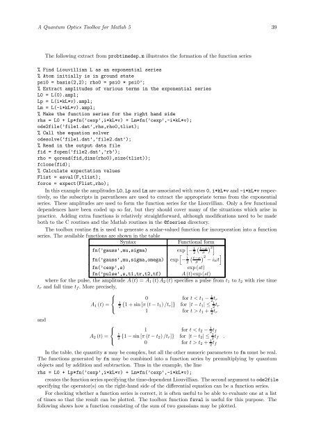
A <strong>Quantum</strong> <strong>Optics</strong> <strong>Toolbox</strong> <strong>for</strong> <strong>Matlab</strong> 5 39The following extract from probtimedep.m illustrates the <strong>for</strong>mation of the function series% Find Liouvillian L as an exponential series% Atom initially is in ground statepsi0 = basis(2,2); rho0 = psi0 * psi0’;% Extract amplitudes of various terms in the exponential seriesL0 = L(0).ampl;Lp = L(i*kL*v).ampl;Lm = L(-i*kL*v).ampl;% Make the function series <strong>for</strong> the right hand siderhs = L0 + Lp*fn(’cexp’,i*kL*v) + Lm*fn(’cexp’,-i*kL*v);ode2file(’file1.dat’,rhs,rho0,tlist);% Call the equation solverodesolve(’file1.dat’,’file2.dat’);% Read in the output data filefid = fopen(’file2.dat’,’rb’);rho = qoread(fid,dims(rho0),size(tlist));fclose(fid);% Calculate expectation valuesFlist = esval(F,tlist);<strong>for</strong>ce = expect(Flist,rho);In this example the amplitudes L0, Lp and Lm are associated with rates 0, i*kL*v and -i*kL*v respectively,so the subscripts in parentheses are used to extract the appropriate terms from the exponentialseries. These amplitudes are used to <strong>for</strong>m the function series <strong>for</strong> the Liouvillian. Only a few functionaldependences have been coded up so far, but they should cover many of the situations which arise inpractice. Adding extra functions is relatively straight<strong>for</strong>ward, although modi…cations need to be madeboth to the C routines and the <strong>Matlab</strong> routines in the @fseries directory.The toolbox routine fn is used to generate a scalar-valued function <strong>for</strong> incorporation into a functionseries. The available functions are shown in the tableSyntaxFunctionalh<strong>for</strong>m¢ 2ifn(’gauss’,mu,sigma)fn(’gauss’,mu,sigma,omega)expexph¡ 1 2¡¡ 1 t¡¹2 ¾¡ t¡¹¾¢ 2¡ i!tifn(’cexp’,s)exp (st)fn(’pulse’,s,t1,tr,t2,tf) A (t)exp(st)where <strong>for</strong> the pulse, the amplitude A (t) =A 1 (t) A 2 (t) speci…es a pulse from t 1 to t 2 with rise timet r and fall time t f : More precisely,8