Bernoulli's lightray solution for the brachistochrone problem from ...
Bernoulli's lightray solution for the brachistochrone problem from ...
Bernoulli's lightray solution for the brachistochrone problem from ...
- No tags were found...

Create successful ePaper yourself
Turn your PDF publications into a flip-book with our unique Google optimized e-Paper software.
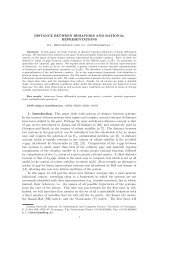
Bernoulli’s <strong>lightray</strong> <strong>solution</strong><strong>for</strong> <strong>the</strong> <strong>brachistochrone</strong> <strong>problem</strong><strong>from</strong> Hamilton’s viewpointHenk BroerJohann Bernoulli Institute <strong>for</strong> Ma<strong>the</strong>matics and Computer ScienceRijksuniversiteit Groningen
Summaryi. Introductionii. Bernoulli’s <strong>solution</strong>iii. Translation into Hamilton’s termsvi. Concluding remarksA study in anachronism...H.H. Goldstine, A History of <strong>the</strong> Calculus of Variations <strong>from</strong> <strong>the</strong> 17th through <strong>the</strong> 19th Century.Studies in <strong>the</strong> History of Ma<strong>the</strong>matics and Physical Sciences 5, Springer 1980J.A. van Maanen, Een Complexe Groo<strong>the</strong>id, leven en werk van Johann Bernoulli. 1667–1748.Epsilon Uitgaven 34 1995D.J. Struik (ed.), A Source Book in Ma<strong>the</strong>matics 1200–1800. Harvard University Press 1969;Princeton University Press 1986
IntroductionJohann Bernoulli (1667 - 1748)‘his’ <strong>brachistochrone</strong> <strong>problem</strong>- Groningen period 1695 – 1705- Acta Eruditorum 1697Opera Johannis Bernoullii. G. Cramer (ed.; 4 delen), Genève 1742
Bernoulli’s <strong>lightray</strong> <strong>solution</strong>Fermat principle of least time <strong>for</strong> light rays optical <strong>solution</strong> in mechanical setting- Discrete approximation in horizontal layerseach layer homogeneous and isotropic refraction index n = 1/v (c = 1)- Fermat principle⇒- inside layer:ray = straight line with velocity v = 1/n- at boundary: Snell’s lawG.W. Leibniz, Nova methodus pro maximis et minimis. Acta Eruditorum 1684. In: D.J. Struik, Asource book in ma<strong>the</strong>matics 1200–1800. Harvard University Press 1969, 271-281
Fermat and Snelln 1 sinα = n 2 sinβProof: Let x = x C indicate position of Ct AC = n 1 |A−C| andt CB = n 2 |C −B|
Fermat and Snell, ctdBy Pythagoras <strong>the</strong>orem:|A−C| = √ x 2 +b 2 , |C −B| =√(a−x) 2 +c 2Differentiatingt AC and t CB w.r.t. x :ddx t AC(x) =ddx t AC(x) = − n 2(a−x)√(a−x) 2 +c 2n 1 x√x 2 +b 2 = n 1 sinα= −n 2 sinβ:ddx (t AC +t CB )(x) = 0 ⇔ n 1 sinα = n 2 sinβ□- locally minimum- globally caustics (think of focal points ellipse)
Bernoulli and Snell- Snell’s law: n j sinα j = n j+1 sinα ′ j- Euclidean geometry: α ′ j = α j+1 Conservation law: n j sinα j = n j+1 sinα j+1just take limits ... inclination α with verticaland conserved quantity nsinα
The cycloid as <strong>brachistochrone</strong>Two conserved quantities as a function ofyS = n(y)sinα(y) (1)E = 1 2 m(v(y))2 +mgy (2)Better look <strong>for</strong> profile α ↦→ (x(α),y(α)) !Theorem.x(α) = x 0 − 14S 2 g (2α−sin(2α))y(α) = y 0 + 14S 2 g cos(2α)Note: E = 1 2 m(v(y 0)) 2 +mgy 0 ,Possible choices: v(y 0 ) = 0 and even y 0 = 0 falling ratev(y) = √ −2gy
A few high school computationsLemma. (abbreviating v ′ = dv/dy)v ′ = − gv(y)andcosα = Sv ′ (y) dydα ,Proof: Differentiate (2) with respect toy and (1) with respect toα□Thusdydαlemma=1Sv ′ (y)cosαlemma= − v(y)Sgvcosα(1)= − 12S 2 gsin(2α) (3)while:dxdα= tanαdydα(3)= − v(y)Sgsinα(1)= − 12S 2 g (1−cos(2α))Integration <strong>the</strong>n gives <strong>the</strong> desired result.Cycloid with radius14S 2 gand rolling angle 2α□
Radius and rolling angleRoll wheel ( radius̺) along ceilingcycloid:x(ϕ) = ̺(ϕ+sinϕ),y(ϕ) = ̺(1−cosϕ)parameterϕcalled rolling angle
Christiaan Huygens (1629-1695)Christiaan Huygens (by Gaspar Netscher)and page <strong>from</strong> Horologium Oscillatorium 1673
Commentary- Challenge in Acta Eruditorum (1697)Many contemporaries published <strong>solution</strong>sNewton’s was anonymous, however,ex ungue leonem cognavi- Isochrony and tautochrony cycloid dynamicsby harmonic oscillationsJ.L. Lagrange, Mécanique Analytique. 4 ed., 2 vols. Gauthier-Villars et fils, Paris, 1888-89
William Rowan Hamilton- Many contributions to ma<strong>the</strong>matics,physics and astronomy ,principle of least actionW.R. Hamilton, Theory of systems of rays. Trans. Roy. Irish Academy 15 (1828), 69-174—, On a general method in dynamics. Phil. Trans. Roy. Soc. Vol. 124 (1834), 247-308; Secondessay on a general method in dynamics. Phil. Trans. Roy. Soc. Vol. 125 (1835), 95-144
Fermat principle revisited- Given curve τ ↦→ q(τ) consider ˙q = dq/dτ anddt = n(q(τ))||˙q(τ)||dτ magic <strong>for</strong>mula- To (locally) minimize ∫ τ 2τ 1n(q(τ))||˙q(τ)||dτ or,ra<strong>the</strong>r and equivalently,I(q) :=∫ τ2τ 112 n2 (q(τ))||˙q(τ)|| 2 dτ- Lagrangian L(q, ˙q) = 1 2 n2 (q)||˙q|| 2(= energy = kinetic energy)
Calculus of variations- If q = (x,y) <strong>the</strong>n Euler–Lagrange equationsddτddτ∂L∂ẋ = ∂L∂x∂L∂ẏ = ∂L∂ynecessary & sufficient <strong>for</strong> local optimality ofI- under small variations ofq,while keeping endpointsq(τ 1 ) andq(τ 2 ) fixed- in current optical setting also minimalL. Euler, Leonhardi Euleri Opera Omnia. 72 vols., Bern 1911-1975J.L. Lagrange, Œuvres. A. Serret and G. Darboux eds., Paris 1867-1892
Hamilton’s canonical <strong>for</strong>malism- Legendre trans<strong>for</strong>mation:R 2 × R 2 → R 2 × R 2 ,(q, ˙q) ↦→ (q,p) with p = n 2 (q)˙q- Hamiltonian H(q,p) = L(q,p/n 2 (q)) = 1n 2 (q) ||p||2Theorem. The <strong>lightray</strong>s are <strong>the</strong> projections of <strong>the</strong><strong>solution</strong>s of <strong>the</strong> canonical equationsto R 2 = {q}˙q j = ∂H∂p j, ṗ j = − ∂H∂q j(j = 1,2)- modern lingo in terms of (co-) tangent bundles
Laws, properties- Energy conservationḢ≡ 0, say H(q,p) = E- q = (x,y) and p x = n 2 (y)ẋ,p y = n 2 (y)ẏH(x,y,p x ,p y ) = 12n 2 (y) (p2 x +p 2 y)- H independent of x (cyclic variable): ṗ x ≡ 0conservation of momentum, sayp x = I- translation symmetry, Noe<strong>the</strong>r principle- conservation ofI √2E(x,y,ẋ,ẏ) = n(y)ẋ√ẋ2+ẏ 2 = n(y)sinα(ẋ,ẏ)(= S <strong>for</strong> Snell, this is familiar !)
Reduction of <strong>the</strong> symmetryTheorem. Given p x = I can reduce to planar systemH I (y,p y ) = 12n 2 (y) p2 y +V I (y) with V I (y) = I22n 2 (y)(effective potential)Reduced system:TakeI ≠ 0ẏ =1n 2 (y) p yṗ y = − n′ (y)n 3 (y) (I2 +p 2 y)
Gravitational refraction indexBack to <strong>brachistochrone</strong> <strong>problem</strong>Gravitational energy 1 2 (v(y))2 +gy = 0 (n(y)) 2 = 1−2gy , <strong>for</strong>y < 0 reduced canonical equationsẏ = −2gyp yṗ y = g(p 2 y +I 2 )Level curve H I (y,p y ) = E has <strong>for</strong>my = − 1 ( ) Eg p 2 y +I 2(4)
Reduced phase-portraitReduced phase-portrait<strong>brachistochrone</strong> <strong>lightray</strong> dynamics
Reconstruction ITime parametrization reduced system,<strong>for</strong> given I ≠ 0 completely determined by E,N- Time parametrizationdτ =dp yg(p 2 y +I 2 ) τ = 1 (gI arctan py)I- Gives parametrization (withp y (0) = 0):p y = Itan(gIτ) (4) y = − EgI 2 cos2 (gIτ) (5)PS: Similar action <strong>for</strong> pendulum system leadsto elliptic integrals ...
Reconstruction IICycloids recovered- I = p x = n 2 (y)ẋ ⇒ẋ =1n 2 (y)(5)I = −2Igy =2EI cos2 (gIτ) = E I (1+cos(2gIτ))- And sox = x 0 + E2gI2(2gIτ +sin(2gIτ))y = − E2gI 2(1+cos(2gIτ))Cycloid radius̺ = E/2gI 2 , rolling angleϕ = 2gIτInclination α = gIτ (proportionality)
Scholium I- Reminds of how Newton ‘principia’ yield <strong>the</strong>Keplerian orbits in central <strong>for</strong>ce field- Nowadays <strong>brachistochrone</strong> <strong>problem</strong> excercise incourse calculus of variations:Look <strong>for</strong> curvey = y(x)arclengthds = √ dx 2 +dy 2 = √ 1+(y ′ ) 2 dxenergy conservation in gravitational fieldso have to optimize... dsdt = √ −2gy
Scholium I: ctd- ... timedt =√1+(y′ ) 2√ −2gy L(y,y ′ ) =√− 1+(y′ ) 22gy- Euler–Lagrange equations ( 1+(y ′ ) 2) y = constantsubstitution of(x,y) = (x(θ),y(θ))again gives cycloid resultV.I. Arnold, Ma<strong>the</strong>matical methods of classical mechanics. GTM 60, Springer 1978, 1989H. Goldstein, Classical mechanics 2nd ed. Addison Wesley 1950, 1980
Scholium II: <strong>lightray</strong>s geodesicsGeorg Friedrich Bernhard Riemann 1826-1866- Riemannian metricG q (˙q 1 , ˙q 2 ) = n 2 (q)〈˙q 1 , ˙q 2 〉,where latter brackets are EuclideannoteL(q, ˙q) = 1 2 G q(˙q, ˙q)- <strong>lightray</strong>s are geodesics of metricGM. Spivak, Differential geometry, Vols. I, II, III. Publish or Perish 1970
Atmospherical optics- blank strip in <strong>the</strong> setting Sun- illusions: fata morgana’s, Nova Zembla phenomenaM.G.J. Minnaert, De Natuurkunde van ’t vrije veld. Vol. 1, Vijfde Editie, ThiemeMeulenhoff1996; The Nature of Light & Colour in <strong>the</strong> Open Air, Dover 1954H.W. Broer, Aardse en hemelse luchtspiegelingen, met Bernoulli,Wegener en Minnaert. To bepublished Epsilon Uitgaven 2013
Arclength cycloidarclengths = s(ϕ) (using Pythagoras):ds = √ dx 2 +dy 2 == √ (dx/dϕ) 2 +(dy/dϕ) 2 dϕ == ̺√2 √ 1+cosϕ dϕ = 2̺cos ϕ 2 dϕ s(ϕ) = 4̺sin ϕ 2
Cycloidal wire profileVertical heighty(ϕ) = 2̺sin 2 ϕ 2 = 18̺(s(ϕ))2 potential energy“V = mgy” : V(s) = mg8̺s2−→ equation of motion beads ′′ = − g4̺s :a harmonic oscillator with ω = √ g/(4̺)Conclusion: cycloid isochronous curve(also tautochronous...)