Chapter 1 Discrete Probability Distributions - DIM

Chapter 1Discrete ProbabilityDistributions1.1 Simulation of Discrete ProbabilitiesProbabilityIn this chapter, we shall first consider chance experiments with a finite number ofpossible outcomes ω 1 , ω 2 , ..., ω n . For example, we roll a die and the possibleoutcomes are 1, 2, 3, 4, 5, 6 corresponding to the side that turns up. We toss a coinwith possible outcomes H (heads) and T (tails).It is frequently useful to be able to refer to an outcome of an experiment. Forexample, we might want to write the mathematical expression which gives the sumof four rolls of a die. To do this, we could let X i , i =1,2,3,4,represent the valuesof the outcomes of the four rolls, and then we could write the expressionX 1 + X 2 + X 3 + X 4for the sum of the four rolls. The X i ’s are called random variables. A random variableis simply an expression whose value is the outcome of a particular experiment.Just as in the case of other types of variables in mathematics, random variables cantake on different values.Let X be the random variable which represents the roll of one die. We shallassign probabilities to the possible outcomes of this experiment. We do this byassigning to each outcome ω j a nonnegative number m(ω j ) in such a way thatm(ω 1 )+m(ω 2 )+···+m(ω 6 )=1.The function m(ω j ) is called the distribution function of the random variable X.For the case of the roll of the die we would assign equal probabilities or probabilities1/6 to each of the outcomes. With this assignment of probabilities, one could writeP (X ≤ 4) = 2 31

2 CHAPTER 1. DISCRETE PROBABILITY DISTRIBUTIONSto mean that the probability is 2/3 that a roll of a die will have a value which doesnot exceed 4.Let Y be the random variable which represents the toss of a coin. In this case,there are two possible outcomes, which we can label as H and T. Unless we havereason to suspect that the coin comes up one way more often than the other way,it is natural to assign the probability of 1/2 to each of the two outcomes.In both of the above experiments, each outcome is assigned an equal probability.This would certainly not be the case in general. For example, if a drug is found tobe effective 30 percent of the time it is used, we might assign a probability .3 thatthe drug is effective the next time it is used and .7 that it is not effective. This lastexample illustrates the intuitive frequency concept of probability. That is, if we havea probability p that an experiment will result in outcome A, then if we repeat thisexperiment a large number of times we should expect that the fraction of times thatA will occur is about p. To check intuitive ideas like this, we shall find it helpful tolook at some of these problems experimentally. We could, for example, toss a coina large number of times and see if the fraction of times heads turns up is about 1/2.We could also simulate this experiment on a computer.SimulationWe want to be able to perform an experiment that corresponds to a given set ofprobabilities; for example, m(ω 1 )=1/2, m(ω 2 )=1/3, and m(ω 3 )=1/6. In thiscase, one could mark three faces of a six-sided die with an ω 1 , two faces with an ω 2 ,and one face with an ω 3 .In the general case we assume that m(ω 1 ), m(ω 2 ), ..., m(ω n ) are all rationalnumbers, with least common denominator n. If n>2, we can imagine a longcylindrical die with a cross-section that is a regular n-gon. If m(ω j )=n j /n, thenwe can label n j of the long faces of the cylinder with an ω j , and if one of the endfaces comes up, we can just roll the die again. If n = 2, a coin could be used toperform the experiment.We will be particularly interested in repeating a chance experiment a large numberof times. Although the cylindrical die would be a convenient way to carry outa few repetitions, it would be difficult to carry out a large number of experiments.Since the modern computer can do a large number of operations in a very shorttime, it is natural to turn to the computer for this task.Random NumbersWe must first find a computer analog of rolling a die. This is done on the computerby means of a random number generator. Depending upon the particular softwarepackage, the computer can be asked for a real number between 0 and 1, or an integerin a given set of consecutive integers. In the first case, the real numbers are chosenin such a way that the probability that the number lies in any particular subintervalof this unit interval is equal to the length of the subinterval. In the second case,each integer has the same probability of being chosen.

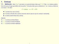
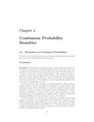
1.1. SIMULATION OF DISCRETE PROBABILITIES 5108642-2-4-6-8-105 10 15 20 25 30 35 40Figure 1.1: Peter’s winnings in 40 plays of heads or tails.One can understand this calculation as follows: The probability that no 6 turnsup on the first toss is (5/6). The probability that no 6 turns up on either of thefirst two tosses is (5/6) 2 . Reasoning in the same way, the probability that no 6turns up on any of the first four tosses is (5/6) 4 . Thus, the probability of at leastone 6 in the first four tosses is 1 − (5/6) 4 . Similarly, for the second bet, with 24rolls, the probability that de Méré wins is 1 − (35/36) 24 = .491, and for 25 rolls itis 1 − (35/36) 25 = .506.Using the rule of thumb mentioned above, it would require 27,000 rolls to have areasonable chance to determine these probabilities with sufficient accuracy to assertthat they lie on opposite sides of .5. It is interesting to ponder whether a gamblercan detect such probabilities with the required accuracy from gambling experience.Some writers on the history of probability suggest that de Méré was, in fact, justinterested in these problems as intriguing probability problems.Example 1.4 (Heads or Tails) For our next example, we consider a problem wherethe exact answer is difficult to obtain but for which simulation easily gives thequalitative results. Peter and Paul play a game called heads or tails. In this game,a fair coin is tossed a sequence of times—we choose 40. Each time a head comes upPeter wins 1 penny from Paul, and each time a tail comes up Peter loses 1 pennyto Paul. For example, if the results of the 40 tosses areTHTHHHHTTHTHHTTHHTTTTHHHTHHTHHHTHHHTTTHH.Peter’s winnings may be graphed as in Figure 1.1.Peter has won 6 pennies in this particular game. It is natural to ask for theprobability that he will win j pennies; here j could be any even number from −40to 40. It is reasonable to guess that the value of j with the highest probabilityis j = 0, since this occurs when the number of heads equals the number of tails.Similarly, we would guess that the values of j with the lowest probabilities arej = ±40.

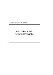
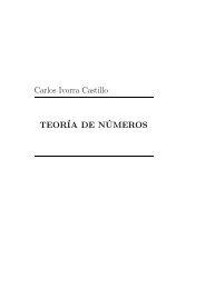
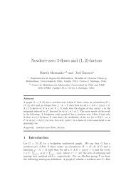
6 CHAPTER 1. DISCRETE PROBABILITY DISTRIBUTIONSA second interesting question about this game is the following: How many timesin the 40 tosses will Peter be in the lead? Looking at the graph of his winnings(Figure 1.1), we see that Peter is in the lead when his winnings are positive, butwe have to make some convention when his winnings are 0 if we want all tosses tocontribute to the number of times in the lead. We adopt the convention that, whenPeter’s winnings are 0, he is in the lead if he was ahead at the previous toss andnot if he was behind at the previous toss. With this convention, Peter is in the lead34 times in our example. Again, our intuition might suggest that the most likelynumber of times to be in the lead is 1/2 of 40, or 20, and the least likely numbersare the extreme cases of 40 or 0.It is easy to settle this by simulating the game a large number of times andkeeping track of the number of times that Peter’s final winnings are j, and thenumber of times that Peter ends up being in the lead by k. The proportions overall games then give estimates for the corresponding probabilities. The programHTSimulation carries out this simulation. Note that when there are an evennumber of tosses in the game, it is possible to be in the lead only an even numberof times. We have simulated this game 10,000 times. The results are shown inFigures 1.2 and 1.3. These graphs, which we call spike graphs, were generatedusing the program Spikegraph. The vertical line, or spike, at position x on thehorizontal axis, has a height equal to the proportion of outcomes which equal x.Our intuition about Peter’s final winnings was quite correct, but our intuition aboutthe number of times Peter was in the lead was completely wrong. The simulationsuggests that the least likely number of times in the lead is 20 and the most likelyis 0 or 40. This is indeed correct, and the explanation for it is suggested by playingthe game of heads or tails with a large number of tosses and looking at a graph ofPeter’s winnings. In Figure 1.4 we show the results of a simulation of the game, for1000 tosses and in Figure 1.5 for 10,000 tosses.In the second example Peter was ahead most of the time. It is a remarkablefact, however, that, if play is continued long enough, Peter’s winnings will continueto come back to 0, but there will be very long times between the times that thishappens. These and related results will be discussed in Chapter 12.✷In all of our examples so far, we have simulated equiprobable outcomes. Weillustrate next an example where the outcomes are not equiprobable.Example 1.5 (Horse Races) Four horses (Acorn, Balky, Chestnut, and Dolby)have raced many times. It is estimated that Acorn wins 30 percent of the time,Balky 40 percent of the time, Chestnut 20 percent of the time, and Dolby 10 percentof the time.We can have our computer carry out one race as follows: Choose a randomnumber x. If x

1.1. SIMULATION OF DISCRETE PROBABILITIES 70.120.10.080.060.040.020-20 -10 0 10 20Figure 1.2: Distribution of winnings.0.120.100.080.060.040.0200 10 20 30 40Figure 1.3: Distribution of number of times in the lead.

8 CHAPTER 1. DISCRETE PROBABILITY DISTRIBUTIONS201000 plays100-10200 400 600 800 1000-20-30-40-50Figure 1.4: Peter’s winnings in 1000 plays of heads or tails.20010000 plays1501005002000 4000 6000 8000 10000Figure 1.5: Peter’s winnings in 10,000 plays of heads or tails.

1.1. SIMULATION OF DISCRETE PROBABILITIES 9of the time. A larger number of races would be necessary to have better agreementwith the past experience. Therefore we ran the program to simulate 1000 raceswith our four horses. Although very tired after all these races, they performed ina manner quite consistent with our estimates of their abilities. Acorn won 29.8percent of the time, Balky 39.4 percent, Chestnut 19.5 percent, and Dolby 11.3percent of the time.The program GeneralSimulation uses this method to simulate repetitions ofan arbitrary experiment with a finite number of outcomes occurring with knownprobabilities.✷Historical RemarksAnyone who plays the same chance game over and over is really carrying out a simulation,and in this sense the process of simulation has been going on for centuries.As we have remarked, many of the early problems of probability might well havebeen suggested by gamblers’ experiences.It is natural for anyone trying to understand probability theory to try simpleexperiments by tossing coins, rolling dice, and so forth. The naturalist Buffon tosseda coin 4040 times, resulting in 2048 heads and 1992 tails. He also estimated thenumber π by throwing needles on a ruled surface and recording how many timesthe needles crossed a line (see Section 2.1). The English biologist W. F. R. Weldon 1recorded 26,306 throws of 12 dice, and the Swiss scientist Rudolf Wolf 2 recorded100,000 throws of a single die without a computer. Such experiments are very timeconsumingand may not accurately represent the chance phenomena being studied.For example, for the dice experiments of Weldon and Wolf, further analysis of therecorded data showed a suspected bias in the dice. The statistician Karl Pearsonanalyzed a large number of outcomes at certain roulette tables and suggested thatthe wheels were biased. He wrote in 1894:Clearly, since the Casino does not serve the valuable end of huge laboratoryfor the preparation of probability statistics, it has no scientificraison d’être. Men of science cannot have their most refined theoriesdisregarded in this shameless manner! The French Government must beurged by the hierarchy of science to close the gaming-saloons; it wouldbe, of course, a graceful act to hand over the remaining resources of theCasino to the Académie des Sciences for the endowment of a laboratoryof orthodox probability; in particular, of the new branch of that study,the application of the theory of chance to the biological problems ofevolution, which is likely to occupy so much of men’s thoughts in thenear future. 3However, these early experiments were suggestive and led to important discoveriesin probability and statistics. They led Pearson to the chi-squared test, which1 T. C. Fry, Probability and Its Engineering Uses, 2nd ed. (Princeton: Van Nostrand, 1965).2 E. Czuber, Wahrscheinlichkeitsrechnung, 3rd ed. (Berlin: Teubner, 1914).3 K. Pearson, “Science and Monte Carlo,” Fortnightly Review, vol. 55 (1894), p. 193; cited inS. M. Stigler, The History of Statistics (Cambridge: Harvard University Press, 1986).

10 CHAPTER 1. DISCRETE PROBABILITY DISTRIBUTIONSis of great importance in testing whether observed data fit a given probability distribution.By the early 1900s it was clear that a better way to generate random numberswas needed. In 1927, L. H. C. Tippett published a list of 41,600 digits obtained byselecting numbers haphazardly from census reports. In 1955, RAND Corporationprinted a table of 1,000,000 random numbers generated from electronic noise. Theadvent of the high-speed computer raised the possibility of generating random numbersdirectly on the computer, and in the late 1940s John von Neumann suggestedthat this be done as follows: Suppose that you want a random sequence of four-digitnumbers. Choose any four-digit number, say 6235, to start. Square this numberto obtain 38,875,225. For the second number choose the middle four digits of thissquare (i.e., 8752). Do the same process starting with 8752 to get the third number,and so forth.More modern methods involve the concept of modular arithmetic. If a is aninteger and m is a positive integer, then by a (mod m) we mean the remainderwhen a is divided by m. For example, 10 (mod 4) = 2, 8 (mod 2) = 0, and soforth. To generate a random sequence X 0 ,X 1 ,X 2 ,... of numbers choose a startingnumber X 0 and then obtain the numbers X n+1 from X n by the formulaX n+1 =(aX n + c) (mod m) ,where a, c, and m are carefully chosen constants. The sequence X 0 ,X 1 ,X 2 ,...is then a sequence of integers between 0 and m − 1. To obtain a sequence of realnumbers in [0, 1), we divide each X j by m. The resulting sequence consists ofrational numbers of the form j/m, where 0 ≤ j ≤ m − 1. Since m is usually avery large integer, we think of the numbers in the sequence as being random realnumbers in [0, 1).For both von Neumann’s squaring method and the modular arithmetic techniquethe sequence of numbers is actually completely determined by the first number.Thus, there is nothing really random about these sequences. However, they producenumbers that behave very much as theory would predict for random experiments.To obtain different sequences for different experiments the initial number X 0 ischosen by some other procedure that might involve, for example, the time of day. 4During the Second World War, physicists at the Los Alamos Scientific Laboratoryneeded to know, for purposes of shielding, how far neutrons travel throughvarious materials. This question was beyond the reach of theoretical calculations.Daniel McCracken, writing in the Scientific American, states:The physicists had most of the necessary data: they knew the averagedistance a neutron of a given speed would travel in a given substancebefore it collided with an atomic nucleus, what the probabilities werethat the neutron would bounce off instead of being absorbed by thenucleus, how much energy the neutron was likely to lose after a given4 For a detailed discussion of random numbers, see D. E. Knuth, The Art of Computer Programming,vol. II (Reading: Addison-Wesley, 1969).

1.1. SIMULATION OF DISCRETE PROBABILITIES 11collision and so on. 5John von Neumann and Stanislas Ulam suggested that the problem be solvedby modeling the experiment by chance devices on a computer. Their work beingsecret, it was necessary to give it a code name. Von Neumann chose the name“Monte Carlo.” Since that time, this method of simulation has been called theMonte Carlo Method.William Feller indicated the possibilities of using computer simulations to illustratebasic concepts in probability in his book Introduction to Probability Theoryand Its Applications. In discussing the problem about the number of times in thelead in the game of “heads or tails” Feller writes:The results concerning fluctuations in coin tossing show that widelyheld beliefs about the law of large numbers are fallacious. These resultsare so amazing and so at variance with common intuition that evensophisticated colleagues doubted that coins actually misbehave as theorypredicts. The record of a simulated experiment is therefore included. 6Feller provides a plot showing the result of 10,000 plays of heads or tails similar tothat in Figure 1.5.The martingale betting system described in Exercise 10 has a long and interestinghistory. Russell Barnhart pointed out to the authors that its use can be tracedback at least to 1754, when Casanova, writing in his memoirs, History of My Life,writesShe [Casanova’s mistress] made me promise to go to the casino [theRidotto in Venice] for money to play in partnership with her. I wentthere and took all the gold I found, and, determinedly doubling mystakes according to the system known as the martingale, I won three orfour times a day during the rest of the Carnival. I never lost the sixthcard. If I had lost it, I should have been out of funds, which amountedto two thousand zecchini. 7Even if there were no zeros on the roulette wheel so the game was perfectly fair,the martingale system, or any other system for that matter, cannot make the gameinto a favorable game. The idea that a fair game remains fair and unfair gamesremain unfair under gambling systems has been exploited by mathematicians toobtain important results in the study of probability. We will introduce the generalconcept of a martingale in Chapter 6.The word martingale itself also has an interesting history. The origin of theword is obscure. The Oxford English Dictionary gives examples of its use in the5 D. D. McCracken, “The Monte Carlo Method,” Scientific American, vol. 192 (May 1955),p. 90.6 W. Feller, Introduction to Probability Theory and its Applications, vol. 1, 3rd ed. (New York:John Wiley & Sons, 1968), p. xi.7 G. Casanova, History of My Life, vol. IV, Chap. 7, trans. W. R. Trask (New York: Harcourt-Brace, 1968), p. 124.

12 CHAPTER 1. DISCRETE PROBABILITY DISTRIBUTIONSearly 1600s and says that its probable origin is the reference in Rabelais’s BookOne, Chapter 19:Everything was done as planned, the only thing being that Gargantuadoubted if they would be able to find, right away, breeches suitable tothe old fellow’s legs; he was doubtful, also, as to what cut would be mostbecoming to the orator—the martingale, which has a draw-bridge effectin the seat, to permit doing one’s business more easily; the sailor-style,which affords more comfort for the kidneys; the Swiss, which is warmeron the belly; or the codfish-tail, which is cooler on the loins. 8In modern uses martingale has several different meanings, all related to holdingdown, in addition to the gambling use. For example, it is a strap on a horse’sharness used to hold down the horse’s head, and also part of a sailing rig used tohold down the bowsprit.The Labouchere system described in Exercise 9 is named after Henry du PreLabouchere (1831–1912), an English journalist and member of Parliament. Labouchereattributed the system to Condorcet. Condorcet (1743–1794) was a politicalleader during the time of the French revolution who was interested in applying probabilitytheory to economics and politics. For example, he calculated the probabilitythat a jury using majority vote will give a correct decision if each juror has thesame probability of deciding correctly. His writings provided a wealth of ideas onhow probability might be applied to human affairs. 9Exercises1 Modify the program CoinTosses to toss a coin n times and print out afterevery 100 tosses the proportion of heads minus 1/2. Do these numbers appearto approach 0 as n increases? Modify the program again to print out, every100 times, both of the following quantities: the proportion of heads minus 1/2,and the number of heads minus half the number of tosses. Do these numbersappear to approach 0 as n increases?2 Modify the program CoinTosses so that it tosses a coin n times and recordswhether or not the proportion of heads is within .1 of .5 (i.e., between .4and .6). Have your program repeat this experiment 100 times. About howlarge must n be so that approximately 95 out of 100 times the proportion ofheads is between .4 and .6?3 In the early 1600s, Galileo was asked to explain the fact that, although thenumber of triples of integers from 1 to 6 with sum 9 is the same as the numberof such triples with sum 10, when three dice are rolled, a 9 seemed to comeup less often than a 10—supposedly in the experience of gamblers.8 Quoted in the Portable Rabelais, ed. S. Putnam (New York: Viking, 1946), p. 113.9 Le Marquise de Condorcet, Essai sur l’Application de l’Analyse à la Probabilité dès DécisionsRendues a la Pluralité des Voix (Paris: Imprimerie Royale, 1785).

1.1. SIMULATION OF DISCRETE PROBABILITIES 13(a) Write a program to simulate the roll of three dice a large number oftimes and keep track of the proportion of times that the sum is 9 andthe proportion of times it is 10.(b) Can you conclude from your simulations that the gamblers were correct?4 In raquetball, a player continues to serve as long as she is winning; a pointis scored only when a player is serving and wins the volley. The first playerto win 21 points wins the game. Assume that you serve first and have aprobability .6 of winning a volley when you serve and probability .5 whenyour opponent serves. Estimate, by simulation, the probability that you willwin a game.5 Consider the bet that all three dice will turn up sixes at least once in n rollsof three dice. Calculate f(n), the probability of at least one triple-six whenthree dice are rolled n times. Determine the smallest value of n necessary fora favorable bet that a triple-six will occur when three dice are rolled n times.(DeMoivre would say it should be about 216 log 2 = 149.7 and so would answer150—see Exercise 1.2.17. Do you agree with him?)6 In Las Vegas, a roulette wheel has 38 slots numbered 0, 00, 1, 2, ..., 36. The0 and 00 slots are green and half of the remaining 36 slots are red and halfare black. A croupier spins the wheel and throws in an ivory ball. If you bet1 dollar on red, you win 1 dollar if the ball stops in a red slot and otherwiseyou lose 1 dollar. Write a program to find the total winnings for a player whomakes 1000 bets on red.7 Another form of bet for roulette is to bet that a specific number (say 17) willturn up. If the ball stops on your number, you get your dollar back plus 35dollars. If not, you lose your dollar. Write a program that will plot yourwinnings when you make 500 plays of roulette at Las Vegas, first when youbet each time on red (see Exercise 6), and then for a second visit to LasVegas when you make 500 plays betting each time on the number 17. Whatdifferences do you see in the graphs of your winnings on these two occasions?8 An astute student noticed that, in our simulation of the game of heads or tails(see Example 1.4), the proportion of times the player is always in the lead isvery close to the proportion of times that the player’s total winnings end up 0.Work out these probabilities by enumeration of all cases for two tosses andfor four tosses, and see if you think that these probabilities are, in fact, thesame.9 The Labouchere system for roulette is played as follows. Write down a list ofnumbers, usually 1, 2, 3, 4. Bet the sum of the first and last, 1 + 4 = 5, onred. If you win, delete the first and last numbers from your list. If you lose,add the amount that you last bet to the end of your list. Then use the newlist and bet the sum of the first and last numbers (if there is only one number,bet that amount). Continue until your list becomes empty. Show that, if this

14 CHAPTER 1. DISCRETE PROBABILITY DISTRIBUTIONShappens, you win the sum, 1+2+3+4=10,ofyouroriginal list. Simulatethis system and see if you do always stop and, hence, always win. If so, whyis this not a foolproof gambling system?10 Another well-known gambling system is the martingale doubling system. Supposethat you are betting on red to turn up in roulette. Every time you win,bet 1 dollar next time. Every time you lose, double your previous bet. Continueto play until you have won at least 5 dollars or you have lost more than100 dollars. Write a program to simulate this system and play it a numberof times and see how you do. In his book The Newcomes, W. M. Thackerayremarks “You have not played as yet? Do not do so; above all avoid amartingale if you do.” 10 Was this good advice?11 Modify the program HTSimulation so that it keeps track of the maximum ofPeter’s winnings in each game of 40 tosses. Have your program print out theproportion of times that your total winnings take on values 0, 2, 4, ..., 40.Calculate the corresponding exact probabilities for games of two tosses andfour tosses.12 In an upcoming national election for the President of the United States, apollster plans to predict the winner of the popular vote by taking a randomsample of 1000 voters and declaring that the winner will be the one obtainingthe most votes in his sample. Suppose that 48 percent of the voters planto vote for the Republican candidate and 52 percent plan to vote for theDemocratic candidate. To get some idea of how reasonable the pollster’splan is, write a program to make this prediction by simulation. Repeat thesimulation 100 times and see how many times the pollster’s prediction wouldcome true. Repeat your experiment, assuming now that 49 percent of thepopulation plan to vote for the Republican candidate; first with a sample of1000 and then with a sample of 3000. (The Gallup Poll uses about 3000.)(This idea is discussed further in Chapter 9, Section 9.1.)13 The psychologist Tversky and his colleagues 11 say that about four out of fivepeople will answer (a) to the following question:A certain town is served by two hospitals. In the larger hospital about 45babies are born each day, and in the smaller hospital 15 babies are born eachday. Although the overall proportion of boys is about 50 percent, the actualproportion at either hospital may be more or less than 50 percent on any day.At the end of a year, which hospital will have the greater number of days onwhich more than 60 percent of the babies born were boys?(a) the large hospital10 W. M. Thackerey, The Newcomes (London: Bradbury and Evans, 1854–55).11 See K. McKean, “Decisions, Decisions,” Discover, June 1985, pp. 22–31. Kevin McKean,Discover Magazine, c○1987 Family Media, Inc. Reprinted with permission. This popular articlereports on the work of Tverksy et. al. in Judgement Under Uncertainty: Heuristics and Biases(Cambridge: Cambridge University Press, 1982).

1.1. SIMULATION OF DISCRETE PROBABILITIES 15(b) the small hospital(c) neither—the number of days will be about the same.Assume that the probability that a baby is a boy is .5 (actual estimates makethis more like .513). Decide, by simulation, what the right answer is to thequestion. Can you suggest why so many people go wrong?14 You are offered the following game. A coin will be tossed until the first timeit comes up heads. If this occurs on the jth toss you are paid 2 j dollars. Youare sure to win at least 2 dollars so you should be willing to pay to play thisgame—but how much? Few people would pay as much as 10 dollars to playthis game. See if you can decide, by simulation, a reasonable amount thatyou would be willing to pay, per game, if you will be allowed to make a largenumber of plays of the game. Does the amount that you would be willing topay per game depend upon the number of plays that you will be allowed?15 Tversky and his colleagues 12 studied the records of 48 of the Philadelphia76ers basketball games in the 1980–81 season to see if a player had timeswhen he was hot and every shot went in, and other times when he was coldand barely able to hit the backboard. The players estimated that they wereabout 25 percent more likely to make a shot after a hit than after a miss.In fact, the opposite was true—the 76ers were 6 percent more likely to scoreafter a miss than after a hit. Tversky reports that the number of hot and coldstreaks was about what one would expect by purely random effects. Assumingthat a player has a fifty-fifty chance of making a shot and makes 20 shots agame, estimate by simulation the proportion of the games in which the playerwill have a streak of 5 or more hits.16 Estimate, by simulation, the average number of children there would be ina family if all people had children until they had a boy. Do the same if allpeople had children until they had at least one boy and at least one girl. Howmany more children would you expect to find under the second scheme thanunder the first in 100,000 families? (Assume that boys and girls are equallylikely.)17 Mathematicians have been known to get some of the best ideas while sitting ina cafe, riding on a bus, or strolling in the park. In the early 1900s the famousmathematician George Pólya lived in a hotel near the woods in Zurich. Heliked to walk in the woods and think about mathematics. Pólya describes thefollowing incident:12 ibid.At the hotel there lived also some students with whom I usuallytook my meals and had friendly relations. On a certain day oneof them expected the visit of his fiancée, what (sic) I knew, butI did not foresee that he and his fiancée would also set out for astroll in the woods, and then suddenly I met them there. And then

16 CHAPTER 1. DISCRETE PROBABILITY DISTRIBUTIONS-3-2-10 1 2 3a. Random walk in one dimension.b. Random walk in two dimensions.c. Random walk in three dimensions.Figure 1.6: Random walk.

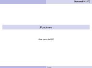
1.1. SIMULATION OF DISCRETE PROBABILITIES 17I met them the same morning repeatedly, I don’t remember howmany times, but certainly much too often and I felt embarrassed:It looked as if I was snooping around which was, I assure you, notthe case. 13This set him to thinking about whether random walkers were destined tomeet.Pólya considered random walkers in one, two, and three dimensions. In onedimension, he envisioned the walker on a very long street. At each intersectionthe walker flips a fair coin to decide which direction to walk next (seeFigure 1.6a). In two dimensions, the walker is walking on a grid of streets, andat each intersection he chooses one of the four possible directions with equalprobability (see Figure 1.6b). In three dimensions (we might better speak ofa random climber), the walker moves on a three-dimensional grid, and at eachintersection there are now six different directions that the walker may choose,each with equal probability (see Figure 1.6c).The reader is referred to Section 12.1, where this and related problems arediscussed.(a) Write a program to simulate a random walk in one dimension startingat 0. Have your program print out the lengths of the times betweenreturns to the starting point (returns to 0). See if you can guess fromthis simulation the answer to the following question: Will the walkeralways return to his starting point eventually or might he drift awayforever?(b) The paths of two walkers in two dimensions who meet after n steps canbe considered to be a single path that starts at (0, 0) and returns to (0, 0)after 2n steps. This means that the probability that two random walkersin two dimensions meet is the same as the probability that a single walkerin two dimensions ever returns to the starting point. Thus the questionof whether two walkers are sure to meet is the same as the question ofwhether a single walker is sure to return to the starting point.Write a program to simulate a random walk in two dimensions and seeif you think that the walker is sure to return to (0, 0). If so, Pólya wouldbe sure to keep meeting his friends in the park. Perhaps by now youhave conjectured the answer to the question: Is a random walker in oneor two dimensions sure to return to the starting point? Pólya answeredthis question for dimensions one, two, and three. He established theremarkable result that the answer is yes in one and two dimensions andno in three dimensions.13 G. Pólya, “Two Incidents,” Scientists at Work: Festschrift in Honour of Herman Wold, ed.T. Dalenius, G. Karlsson, and S. Malmquist (Uppsala: Almquist & Wiksells Boktryckeri AB,1970).

18 CHAPTER 1. DISCRETE PROBABILITY DISTRIBUTIONS(c) Write a program to simulate a random walk in three dimensions and seewhether, from this simulation and the results of (a) and (b), you couldhave guessed Pólya’s result.1.2 Discrete Probability DistributionsIn this book we shall study many different experiments from a probabilistic point ofview. What is involved in this study will become evident as the theory is developedand examples are analyzed. However, the overall idea can be described and illustratedas follows: to each experiment that we consider there will be associated arandom variable, which represents the outcome of any particular experiment. Theset of possible outcomes is called the sample space. In the first part of this section,we will consider the case where the experiment has only finitely many possible outcomes,i.e., the sample space is finite. We will then generalize to the case that thesample space is either finite or countably infinite. This leads us to the followingdefinition.Random Variables and Sample SpacesDefinition 1.1 Suppose we have an experiment whose outcome depends on chance.We represent the outcome of the experiment by a capital Roman letter, such as X,called a random variable. The sample space of the experiment is the set of allpossible outcomes. If the sample space is either finite or countably infinite, therandom variable is said to be discrete.✷We generally denote a sample space by the capital Greek letter Ω. As stated above,in the correspondence between an experiment and the mathematical theory by whichit is studied, the sample space Ω corresponds to the set of possible outcomes of theexperiment.We now make two additional definitions. These are subsidiary to the definitionof sample space and serve to make precise some of the common terminology usedin conjunction with sample spaces. First of all, we define the elements of a samplespace to be outcomes. Second, each subset of a sample space is defined to be anevent. Normally, we shall denote outcomes by lower case letters and events bycapital letters.Example 1.6 A die is rolled once. We let X denote the outcome of this experiment.Then the sample space for this experiment is the 6-element setΩ={1,2,3,4,5,6},where each outcome i, for i = 1, ..., 6, corresponds to the number of dots on theface which turns up. The eventE = {2, 4, 6}

1.2. DISCRETE PROBABILITY DISTRIBUTIONS 19corresponds to the statement that the result of the roll is an even number. Theevent E can also be described by saying that X is even. Unless there is reason tobelieve the die is loaded, the natural assumption is that every outcome is equallylikely. Adopting this convention means that we assign a probability of 1/6 to eachof the six outcomes, i.e., m(i) =1/6, for 1 ≤ i ≤ 6.✷Distribution FunctionsWe next describe the assignment of probabilities. The definitions are motivated bythe example above, in which we assigned to each outcome of the sample space anonnegative number such that the sum of the numbers assigned is equal to 1.Definition 1.2 Let X be a random variable which denotes the value of the outcomeof a certain experiment, and assume that this experiment has only finitelymany possible outcomes. Let Ω be the sample space of the experiment (i.e., theset of all possible values of X, or equivalently, the set of all possible outcomes ofthe experiment.) A distribution function for X is a real-valued function m whosedomain is Ω and which satisfies:1. m(ω) ≥ 0 , for all ω ∈ Ω , and2.∑ω∈Ωm(ω) =1.For any subset E of Ω, we define the probability of E to be the number P (E) givenbyP (E) =ω∈Em(ω).∑✷Example 1.7 Consider an experiment in which a coin is tossed twice. Let X bethe random variable which corresponds to this experiment. We note that there areseveral ways to record the outcomes of this experiment. We could, for example,record the two tosses, in the order in which they occurred. In this case, we haveΩ={HH,HT,TH,TT}. We could also record the outcomes by simply noting thenumber of heads that appeared. In this case, we have Ω ={0,1,2}. Finally, we couldrecord the two outcomes, without regard to the order in which they occurred. Inthis case, we have Ω ={HH,HT,TT}.We will use, for the moment, the first of the sample spaces given above. Wewill assume that all four outcomes are equally likely, and define the distributionfunction m(ω) bym(HH) = m(HT) = m(TH) = m(TT) = 1 4 .

20 CHAPTER 1. DISCRETE PROBABILITY DISTRIBUTIONSLet E ={HH,HT,TH} be the event that at least one head comes up. Then, theprobability of E can be calculated as follows:P (E) = m(HH) + m(HT) + m(TH)= 1 4 + 1 4 + 1 4 = 3 4 .Similarly, if F ={HH,HT} is the event that heads comes up on the first toss,then we haveP (F ) = m(HH) + m(HT)= 1 4 + 1 4 = 1 2 . ✷Example 1.8 (Example 1.6 continued) The sample space for the experiment inwhich the die is rolled is the 6-element set Ω = {1, 2, 3, 4, 5, 6}. We assumed thatthe die was fair, and we chose the distribution function defined bym(i) = 1 , for i =1,...,6 .6If E is the event that the result of the roll is an even number, then E = {2, 4, 6}andP (E) = m(2) + m(4) + m(6)= 1 6 + 1 6 + 1 6 = 1 2 . ✷Notice that it is an immediate consequence of the above definitions that, forevery ω ∈ Ω,P ({ω}) =m(ω).That is, the probability of the elementary event {ω}, consisting of a single outcomeω, is equal to the value m(ω) assigned to the outcome ω by the distribution function.Example 1.9 Three people, A, B, and C, are running for the same office, and weassume that one and only one of them wins. The sample space may be taken as the3-element set Ω ={A,B,C} where each element corresponds to the outcome of thatcandidate’s winning. Suppose that A and B have the same chance of winning, butthat C has only 1/2 the chance of A or B. Then we assignm(A) = m(B)=2m(C) .Sincem(A) + m(B) + m(C)=1,

1.2. DISCRETE PROBABILITY DISTRIBUTIONS 21we see that2m(C)+2m(C) + m(C)=1,which implies that 5m(C) = 1. Hence,m(A) = 2 5 , m(B) = 2 5 , m(C) = 1 5 .Let E be the event that either A or C wins. Then E ={A,C}, andP (E) =m(A) + m(C) = 2 5 + 1 5 = 3 5 .In many cases, events can be described in terms of other events through the useof the standard constructions of set theory. We will briefly review the definitions ofthese constructions. The reader is referred to Figure 1.7 for Venn diagrams whichillustrate these constructions.Let A and B be two sets. Then the union of A and B is the setThe intersection of A and B is the setThe difference of A and B is the setA ∪ B = {x | x ∈ A or x ∈ B} .A ∩ B = {x | x ∈ A and x ∈ B} .A − B = {x | x ∈ A and x ∉ B} .The set A is a subset of B, written A ⊂ B, if every element of A is also an elementof B. Finally, the complement of A is the setà = {x | x ∈ Ω and x ∉ A} .The reason that these constructions are important is that it is typically thecase that complicated events described in English can be broken down into simplerevents using these constructions. For example, if A is the event that “it will snowtomorrow and it will rain the next day,” B is the event that “it will snow tomorrow,”and C is the event that “it will rain two days from now,” then A is the intersectionof the events B and C. Similarly, if D is the event that “it will snow tomorrow orit will rain the next day,” then D = B ∪ C. (Note that care must be taken here,because sometimes the word “or” in English means that exactly one of the twoalternatives will occur. The meaning is usually clear from context. In this book,we will always use the word “or” in the inclusive sense, i.e., A or B means that atleast one of the two events A, B is true.) The event ˜B is the event that “it will notsnow tomorrow.” Finally, if E is the event that “it will snow tomorrow but it willnot rain the next day,” then E = B − C.✷

⊃⊃22 CHAPTER 1. DISCRETE PROBABILITY DISTRIBUTIONSA BA BAAB∼A B A B AA BFigure 1.7: Basic set operations.PropertiesTheorem 1.1 The probabilities assigned to events by a distribution function on asample space Ω satisfy the following properties:1. P (E) ≥ 0 for every E ⊂ Ω.2. P (Ω)=1.3. If E ⊂ F ⊂ Ω, then P (E) ≤ P (F ).4. If A and B are disjoint subsets of Ω, then P (A ∪ B) =P(A)+P(B).5. P (Ã) =1−P(A) for every A ⊂ Ω.Proof. For any event E the probability P (E) is determined from the distributionm byP (E) =ω∈Em(ω),∑for every E ⊂ Ω. Since the function m is nonnegative, it follows that P (E) is alsononnegative. Thus, Property 1 is true.Property 2 is proved by the equationsP (Ω) = ∑ ω∈Ωm(ω) =1.Suppose that E ⊂ F ⊂ Ω. Then every element ω that belongs to E also belongsto F . Therefore,∑m(ω) ,m(ω) ≤ ∑ω∈E ω∈Fsince each term in the left-hand sum is in the right-hand sum, and all the terms inboth sums are non-negative. This implies thatand Property 3 is proved.P (E) ≤ P (F ) ,

1.2. DISCRETE PROBABILITY DISTRIBUTIONS 23Suppose next that A and B are disjoint subsets of Ω. Then every element ω ofA ∪ B lies either in A and not in B or in B and not in A. It follows thatP (A ∪ B)= ∑ ω∈A∪B m(ω)=∑ ω∈A m(ω)+∑ ω∈B m(ω)=P(A)+P(B),and Property 4 is proved.Finally, to prove Property 5, consider the disjoint unionΩ=A∪Ã.Since P (Ω) = 1, the property of disjoint additivity (Property 4) implies that1=P(A)+P(Ã),whence P (Ã) =1−P(A).✷It is important to realize that Property 1 in Theorem 1.1 can be extended tomore than two sets. The general finite additivity property is given by the followingtheorem.Theorem 1.2 If A 1 , ..., A n are pairwise disjoint subsets of Ω (i.e., no two of theA i ’s have an element in common), thenP (A 1 ∪···∪A n )=n∑P (A i ) .i=1Proof. Let ω be any element in the unionA 1 ∪···∪A n .Then m(ω) occurs exactly once on each side of the equality in the statement of thetheorem.✷We shall often use the following consequence of the above theorem.Theorem 1.3 Let A 1 , ..., A n be pairwise disjoint events with Ω = A 1 ∪···∪A n ,and let E be any event. ThenP (E) =n∑P (E ∩ A i ) .i=1Proof. The sets E ∩ A 1 , ..., E ∩A n are pairwise disjoint, and their union is theset E. The result now follows from Theorem 1.2.✷

24 CHAPTER 1. DISCRETE PROBABILITY DISTRIBUTIONSCorollary 1.1 For any two events A and B,P (A) =P(A∩B)+P(A∩ ˜B).Property 4 can be generalized in another way. Suppose that A and B are subsetsof Ω which are not necessarily disjoint. Then:✷Theorem 1.4 If A and B are subsets of Ω, thenP (A ∪ B) =P(A)+P(B)−P(A∩B). (1.1)Proof. The left side of Equation 1.1 is the sum of m(ω) for ω in either A or B. Wemust show that the right side of Equation 1.1 also adds m(ω) for ω in A or B. Ifωis in exactly one of the two sets, then it is counted in only one of the three termson the right side of Equation 1.1. If it is in both A and B, it is added twice fromthe calculations of P (A) and P (B) and subtracted once for P (A ∩ B). Thus it iscounted exactly once by the right side. Of course, if A ∩ B = ∅, then Equation 1.1reduces to Property 4. (Equation 1.1 can also be generalized; see Theorem 3.8.) ✷Tree DiagramsExample 1.10 Let us illustrate the properties of probabilities of events in termsof three tosses of a coin. When we have an experiment which takes place in stagessuch as this, we often find it convenient to represent the outcomes by a tree diagramas shown in Figure 1.8.A path through the tree corresponds to a possible outcome of the experiment.For the case of three tosses of a coin, we have eight paths ω 1 , ω 2 , ..., ω 8 and,assuming each outcome to be equally likely, we assign equal weight, 1/8, to eachpath. Let E be the event “at least one head turns up.” Then Ẽ is the event ”noheads turn up.” This event occurs for only one outcome, namely, ω 8 = TTT. Thus,Ẽ = {TTT} and we haveBy Property 5 of Theorem 1.1,P (Ẽ) =P({TTT}) =m(TTT) = 1 8 .P (E) =1−P(Ẽ)=1−1 8 =7 8 .Note that we shall often find it is easier to compute the probability that an eventdoes not happen rather than the probability that it does. We then use Property 5to obtain the desired probability.

1.2. DISCRETE PROBABILITY DISTRIBUTIONS 25First toss Second toss Third toss OutcomeHω1HTω2HTHTωω34(Start)THTHTHωωω567Tω8Figure 1.8: Tree diagram for three tosses of a coin.Let A be the event “the first outcome is a head,” and B the event “the secondoutcome is a tail.” By looking at the paths in Figure 1.8, we see thatP (A) =P(B)= 1 2 .Moreover, A ∩ B = {ω 3 ,ω 4 }, and so P (A ∩ B) =1/4.Using Theorem 1.4, we obtainSince A ∪ B is the 6-element set,P (A ∪ B) = P(A)+P(B)−P(A∩B)= 1 2 +1 2 −1 4 = 3 4 .A ∪ B = {HHH,HHT,HTH,HTT,TTH,TTT} ,we see that we obtain the same result by direct enumeration.✷In our coin tossing examples and in the die rolling example, we have assignedan equal probability to each possible outcome of the experiment. Corresponding tothis method of assigning probabilities, we have the following definitions.Uniform DistributionDefinition 1.3 The uniform distribution on a sample space Ω containing n elementsis the function m defined bym(ω) = 1 n ,for every ω ∈ Ω.✷

26 CHAPTER 1. DISCRETE PROBABILITY DISTRIBUTIONSIt is important to realize that when an experiment is analyzed to describe itspossible outcomes, there is no single correct choice of sample space. For the experimentof tossing a coin twice in Example 1.2, we selected the 4-element setΩ={HH,HT,TH,TT} as a sample space and assigned the uniform distribution function.These choices are certainly intuitively natural. On the other hand, for somepurposes it may be more useful to consider the 3-element sample space ¯Ω ={0,1,2}in which 0 is the outcome “no heads turn up,” 1 is the outcome “exactly one headturns up,” and 2 is the outcome “two heads turn up.” The distribution function ¯mon ¯Ω defined by the equations¯m(0) = 1 4 , ¯m(1) = 1 2 , ¯m(2) = 1 4is the one corresponding to the uniform probability density on the original samplespace Ω. Notice that it is perfectly possible to choose a different distribution function.For example, we may consider the uniform distribution function on ¯Ω, whichis the function ¯q defined by¯q(0) = ¯q(1) = ¯q(2) = 1 3 .Although ¯q is a perfectly good distribution function, it is not consistent with observeddata on coin tossing.Example 1.11 Consider the experiment that consists of rolling a pair of dice. Wetake as the sample space Ω the set of all ordered pairs (i, j) of integers with 1 ≤ i ≤ 6and 1 ≤ j ≤ 6. Thus,Ω={(i, j) :1≤i, j ≤ 6 } .(There is at least one other “reasonable” choice for a sample space, namely the setof all unordered pairs of integers, each between 1 and 6. For a discussion of whywe do not use this set, see Example 3.14.) To determine the size of Ω, we notethat there are six choices for i, and for each choice of i there are six choices for j,leading to 36 different outcomes. Let us assume that the dice are not loaded. Inmathematical terms, this means that we assume that each of the 36 outcomes isequally likely, or equivalently, that we adopt the uniform distribution function onΩ by settingm((i, j)) = 1 36 , 1 ≤ i, j ≤ 6 .What is the probability of getting a sum of 7 on the roll of two dice—or getting asum of 11? The first event, denoted by E, is the subsetA sum of 11 is the subset F given byE = {(1, 6), (6, 1), (2, 5), (5, 2), (3, 4), (4, 3)} .F = {(5, 6), (6, 5)} .Consequently,P (E) = ∑ ω∈E m(ω)=6· 136 = 1 6 ,P (F )= ∑ ω∈F m(ω)=2· 136 = 118 .

1.2. DISCRETE PROBABILITY DISTRIBUTIONS 27What is the probability of getting neither snakeeyes (double ones) nor boxcars(double sixes)? The event of getting either one of these two outcomes is the setE = {(1, 1), (6, 6)} .Hence, the probability of obtaining neither is given by2P (Ẽ) =1−P(E)=1−36 = 1718 . ✷In the above coin tossing and the dice rolling experiments, we have assigned anequal probability to each outcome. That is, in each example, we have chosen theuniform distribution function. These are the natural choices provided the coin is afair one and the dice are not loaded. However, the decision as to which distributionfunction to select to describe an experiment is not a part of the basic mathematicaltheory of probability. The latter begins only when the sample space and thedistribution function have already been defined.Determination of ProbabilitiesIt is important to consider ways in which probability distributions are determinedin practice. One way is by symmetry. For the case of the toss of a coin, we do notsee any physical difference between the two sides of a coin that should affect thechance of one side or the other turning up. Similarly, with an ordinary die thereis no essential difference between any two sides of the die, and so by symmetry weassign the same probability for any possible outcome. In general, considerationsof symmetry often suggest the uniform distribution function. Care must be usedhere. We should not always assume that, just because we do not know any reasonto suggest that one outcome is more likely than another, it is appropriate to assignequal probabilities. For example, consider the experiment of guessing the sex ofa newborn child. It has been observed that the proportion of newborn childrenwho are boys is about .513. Thus, it is more appropriate to assign a distributionfunction which assigns probability .513 to the outcome boy and probability .487 tothe outcome girl than to assign probability 1/2 to each outcome. This is an examplewhere we use statistical observations to determine probabilities. Note that theseprobabilities may change with new studies and may vary from country to country.Genetic engineering might even allow an individual to influence this probability fora particular case.OddsStatistical estimates for probabilities are fine if the experiment under considerationcan be repeated a number of times under similar circumstances. However, assumethat, at the beginning of a football season, you want to assign a probability to theevent that Dartmouth will beat Harvard. You really do not have data that relates tothis year’s football team. However, you can determine your own personal probability

28 CHAPTER 1. DISCRETE PROBABILITY DISTRIBUTIONSby seeing what kind of a bet you would be willing to make. For example, supposethat you are willing to make a 1 dollar bet giving 2 to 1 odds that Dartmouth willwin. Then you are willing to pay 2 dollars if Dartmouth loses in return for receiving1 dollar if Dartmouth wins. This means that you think the appropriate probabilityfor Dartmouth winning is 2/3.Let us look more carefully at the relation between odds and probabilities. Supposethat we make a bet at r to 1 odds that an event E occurs. This means thatwe think that it is r times as likely that E will occur as that E will not occur. Ingeneral, r to s odds will be taken to mean the same thing as r/s to 1, i.e., the ratiobetween the two numbers is the only quantity of importance when stating odds.Nowifitisrtimes as likely that E will occur as that E will not occur, then theprobability that E occurs must be r/(r + 1), since we haveP (E) =rP(Ẽ)andP (E)+P(Ẽ)=1.In general, the statement that the odds are r to s in favor of an event E occurringis equivalent to the statement thatP (E) ==r/s(r/s)+1rr+s .If we let P (E) =p, then the above equation can easily be solved for r/s in terms ofp; we obtain r/s = p/(1 − p). We summarize the above discussion in the followingdefinition.Definition 1.4 If P (E) =p, the odds in favor of the event E occurring are r : s (rto s) where r/s = p/(1 − p). If r and s are given, then p can be found by using theequation p = r/(r + s).✷Example 1.12 (Example 1.9 continued) In Example 1.9 we assigned probability1/5 to the event that candidate C wins the race. Thus the odds in favor of Cwinning are 1/5 :4/5. These odds could equally well have been written as 1 : 4,2 : 8, and so forth. A bet that C wins is fair if we receive 4 dollars if C wins andpay 1 dollar if C loses.✷Infinite Sample SpacesIf a sample space has an infinite number of points, then the way that a distributionfunction is defined depends upon whether or not the sample space is countable. Asample space is countably infinite if the elements can be counted, i.e., can be putin one-to-one correspondence with the positive integers, and uncountably infinite

1.2. DISCRETE PROBABILITY DISTRIBUTIONS 29otherwise. Infinite sample spaces require new concepts in general (see Chapter 2),but countably infinite spaces do not. IfΩ={ω 1 ,ω 2 ,ω 3 ,...}is a countably infinite sample space, then a distribution function is defined exactlyas in Definition 1.2, except that the sum must now be a convergent infinite sum.Theorem 1.1 is still true, as are its extensions Theorems 1.2 and 1.4. One thing wecannot do on a countably infinite sample space that we could do on a finite samplespace is to define a uniform distribution function as in Definition 1.3. You are askedin Exercise 20 to explain why this is not possible.Example 1.13 A coin is tossed until the first time that a head turns up. Let theoutcome of the experiment, ω, be the first time that a head turns up. Then thepossible outcomes of our experiment areΩ={1,2,3,...} .Note that even though the coin could come up tails every time we have not allowedfor this possibility. We will explain why in a moment. The probability that headscomes up on the first toss is 1/2. The probability that tails comes up on the firsttoss and heads on the second is 1/4. The probability that we have two tails followedby a head is 1/8, and so forth. This suggests assigning the distribution functionm(n) =1/2 n for n = 1, 2, 3, .... To see that this is a distribution function wemust show that∑m(ω) = 1 2 +1 4 +1 8 +···=1.ωThat this is true follows from the formula for the sum of a geometric series,1+r+r 2 +r 3 +···= 11−r ,orr + r 2 + r 3 + r 4 + ···=r1−r , (1.2)for −1

30 CHAPTER 1. DISCRETE PROBABILITY DISTRIBUTIONSHistorical RemarksAn interesting question in the history of science is: Why was probability not developeduntil the sixteenth century? We know that in the sixteenth century problemsin gambling and games of chance made people start to think about probability. Butgambling and games of chance are almost as old as civilization itself. In ancientEgypt (at the time of the First Dynasty, ca. 3500 B.C.) a game now called “Houndsand Jackals” was played. In this game the movement of the hounds and jackals wasbased on the outcome of the roll of four-sided dice made out of animal bones calledastragali. Six-sided dice made of a variety of materials date back to the sixteenthcentury B.C. Gambling was widespread in ancient Greece and Rome. Indeed, in theRoman Empire it was sometimes found necessary to invoke laws against gambling.Why, then, were probabilities not calculated until the sixteenth century?Several explanations have been advanced for this late development. One is thatthe relevant mathematics was not developed and was not easy to develop. Theancient mathematical notation made numerical calculation complicated, and ourfamiliar algebraic notation was not developed until the sixteenth century. However,as we shall see, many of the combinatorial ideas needed to calculate probabilitieswere discussed long before the sixteenth century. Since many of the chance eventsof those times had to do with lotteries relating to religious affairs, it has beensuggested that there may have been religious barriers to the study of chance andgambling. Another suggestion is that a stronger incentive, such as the developmentof commerce, was necessary. However, none of these explanations seems completelysatisfactory, and people still wonder why it took so long for probability to be studiedseriously. An interesting discussion of this problem can be found in Hacking. 14The first person to calculate probabilities systematically was Gerolamo Cardano(1501–1576) in his book Liber de Ludo Aleae. This was translated from the Latinby Gould and appears in the book Cardano: The Gambling Scholar by Ore. 15 Oreprovides a fascinating discussion of the life of this colorful scholar with accountsof his interests in many different fields, including medicine, astrology, and mathematics.You will also find there a detailed account of Cardano’s famous battle withTartaglia over the solution to the cubic equation.In his book on probability Cardano dealt only with the special case that we havecalled the uniform distribution function. This restriction to equiprobable outcomeswas to continue for a long time. In this case Cardano realized that the probabilitythat an event occurs is the ratio of the number of favorable outcomes to the totalnumber of outcomes.Many of Cardano’s examples dealt with rolling dice. Here he realized that theoutcomes for two rolls should be taken to be the 36 ordered pairs (i, j) rather thanthe 21 unordered pairs. This is a subtle point that was still causing problems muchlater for other writers on probability. For example, in the eighteenth century thefamous French mathematician d’Alembert, author of several works on probability,claimed that when a coin is tossed twice the number of heads that turn up would14 I. Hacking, The Emergence of Probability (Cambridge: Cambridge University Press, 1975).15 O. Ore, Cardano: The Gambling Scholar (Princeton: Princeton University Press, 1953).

1.2. DISCRETE PROBABILITY DISTRIBUTIONS 31be 0, 1, or 2, and hence we should assign equal probabilities for these three possibleoutcomes. 16 Cardano chose the correct sample space for his dice problems andcalculated the correct probabilities for a variety of events.Cardano’s mathematical work is interspersed with a lot of advice to the potentialgambler in short paragraphs, entitled, for example: “Who Should Play and When,”“Why Gambling Was Condemned by Aristotle,” “Do Those Who Teach Also PlayWell?” and so forth. In a paragraph entitled “The Fundamental Principle of Gambling,”Cardano writes:The most fundamental principle of all in gambling is simply equal conditions,e.g., of opponents, of bystanders, of money, of situation, of thedice box, and of the die itself. To the extent to which you depart fromthat equality, if it is in your opponent’s favor, you are a fool, and if inyour own, you are unjust. 17Cardano did make mistakes, and if he realized it later he did not go back andchange his error. For example, for an event that is favorable in three out of fourcases, Cardano assigned the correct odds 3 : 1 that the event will occur. But then heassigned odds by squaring these numbers (i.e., 9 : 1) for the event to happen twice ina row. Later, by considering the case where the odds are 1 : 1, he realized that thiscannot be correct and was led to the correct result that when f out of n outcomesare favorable, the odds for a favorable outcome twice in a row are f 2 : n 2 − f 2 . Orepoints out that this is equivalent to the realization that if the probability that anevent happens in one experiment is p, the probability that it happens twice is p 2 .Cardano proceeded to establish that for three successes the formula should be p 3and for four successes p 4 , making it clear that he understood that the probabilityis p n for n successes in n independent repetitions of such an experiment. This willfollow from the concept of independence that we introduce in Section 4.1.Cardano’s work was a remarkable first attempt at writing down the laws ofprobability, but it was not the spark that started a systematic study of the subject.This came from a famous series of letters between Pascal and Fermat. This correspondencewas initiated by Pascal to consult Fermat about problems he had beengiven by Chevalier de Méré, a well-known writer, a prominent figure at the court ofLouis XIV, and an ardent gambler.The first problem de Méré posed was a dice problem. The story goes that he hadbeen betting that at least one six would turn up in four rolls of a die and winningtoo often, so he then bet that a pair of sixes would turn up in 24 rolls of a pairof dice. The probability of a six with one die is 1/6 and, by the product law forindependent experiments, the probability of two sixes when a pair of dice is thrownis (1/6)(1/6)=1/36. Ore 18 claims that a gambling rule of the time suggested that,since four repetitions was favorable for the occurrence of an event with probability1/6, for an event six times as unlikely, 6 · 4 = 24 repetitions would be sufficient for16 J. d’Alembert, “Croix ou Pile,” in L’Encyclopédie, ed. Diderot, vol. 4 (Paris, 1754).17 O. Ore, op. cit., p. 189.18 O. Ore, “Pascal and the Invention of Probability Theory,” American Mathematics Monthly,vol. 67 (1960), pp. 409–419.

32 CHAPTER 1. DISCRETE PROBABILITY DISTRIBUTIONSa favorable bet. Pascal showed, by exact calculation, that 25 rolls are required fora favorable bet for a pair of sixes.The second problem was a much harder one: it was an old problem and concernedthe determination of a fair division of the stakes in a tournament when theseries, for some reason, is interrupted before it is completed. This problem is nowreferred to as the problem of points. The problem had been a standard problem inmathematical texts; it appeared in Fra Luca Paccioli’s book summa de Arithmetica,Geometria, Proportioni et Proportionalità, printed in Venice in 1494, 19 in the form:A team plays ball such that a total of 60 points are required to win thegame, and each inning counts 10 points. The stakes are 10 ducats. Bysome incident they cannot finish the game and one side has 50 pointsand the other 20. One wants to know what share of the prize moneybelongs to each side. In this case I have found that opinions differ fromone to another but all seem to me insufficient in their arguments, but Ishall state the truth and give the correct way.Reasonable solutions, such as dividing the stakes according to the ratio of gameswon by each player, had been proposed, but no correct solution had been found atthe time of the Pascal-Fermat correspondence. The letters deal mainly with theattempts of Pascal and Fermat to solve this problem. Blaise Pascal (1623–1662)was a child prodigy, having published his treatise on conic sections at age sixteen,and having invented a calculating machine at age eighteen. At the time of theletters, his demonstration of the weight of the atmosphere had already establishedhis position at the forefront of contemporary physicists. Pierre de Fermat (1601–1665) was a learned jurist in Toulouse, who studied mathematics in his spare time.He has been called by some the prince of amateurs and one of the greatest puremathematicians of all times.The letters, translated by Maxine Merrington, appear in Florence David’s fascinatinghistorical account of probability, Games, Gods and Gambling. 20 In a letterdated Wednesday, 29th July, 1654, Pascal writes to Fermat:Sir,Like you, I am equally impatient, and although I am again ill in bed,I cannot help telling you that yesterday evening I received from M. deCarcavi your letter on the problem of points, which I admire more thanI can possibly say. I have not the leisure to write at length, but, in aword, you have solved the two problems of points, one with dice and theother with sets of games with perfect justness; I am entirely satisfiedwith it for I do not doubt that I was in the wrong, seeing the admirableagreement in which I find myself with you now. . .Your method is very sound and is the one which first came to my mindin this research; but because the labour of the combination is excessive,I have found a short cut and indeed another method which is much19 ibid., p. 414.20 F. N. David, Games, Gods and Gambling (London: G. Griffin, 1962), p. 230 ff.

1.2. DISCRETE PROBABILITY DISTRIBUTIONS 3330 0 028 16 32 64Number of gamesB has won120 32 48 64032 44 56640 1 2 3Number of gamesA has wonFigure 1.9: Pascal’s table.quicker and neater, which I would like to tell you here in a few words:for henceforth I would like to open my heart to you, if I may, as I am sooverjoyed with our agreement. I see that truth is the same in Toulouseas in Paris.Here, more or less, is what I do to show the fair value of each game,when two opponents play, for example, in three games and each personhas staked 32 pistoles.Let us say that the first man had won twice and the other once; nowthey play another game, in which the conditions are that, if the firstwins, he takes all the stakes; that is 64 pistoles; if the other wins it,then they have each won two games, and therefore, if they wish to stopplaying, they must each take back their own stake, that is, 32 pistoleseach.Then consider, Sir, if the first man wins, he gets 64 pistoles; if he loseshe gets 32. Thus if they do not wish to risk this last game but wish toseparate without playing it, the first man must say: ‘I am certain to get32 pistoles, even if I lost I still get them; but as for the other 32, perhapsI will get them, perhaps you will get them, the chances are equal. Letus then divide these 32 pistoles in half and give one half to me as wellas my 32 which are mine for sure.’ He will then have 48 pistoles and theother 16. . .Pascal’s argument produces the table illustrated in Figure 1.9 for the amountdue player A at any quitting point.Each entry in the table is the average of the numbers just above and to the rightof the number. This fact, together with the known values when the tournament iscompleted, determines all the values in this table. If player A wins the first game,

34 CHAPTER 1. DISCRETE PROBABILITY DISTRIBUTIONSthen he needs two games to win and B needs three games to win; and so, if thetounament is called off, A should receive 44 pistoles.The letter in which Fermat presented his solution has been lost; but fortunately,Pascal describes Fermat’s method in a letter dated Monday, 24th August, 1654.From Pascal’s letter: 21This is your procedure when there are two players: If two players, playingseveral games, find themselves in that position when the first manneeds two games and second needs three, then to find the fair divisionof stakes, you say that one must know in how many games the play willbe absolutely decided.It is easy to calculate that this will be in four games, from which you canconclude that it is necessary to see in how many ways four games can bearranged between two players, and one must see how many combinationswould make the first man win and how many the second and to shareout the stakes in this proportion. I would have found it difficult tounderstand this if I had not known it myself already; in fact you hadexplained it with this idea in mind.Fermat realized that the number of ways that the game might be finished maynot be equally likely. For example, if A needs two more games and B needs three towin, two possible ways that the tournament might go for A to win are WLW andLWLW. These two sequences do not have the same chance of occurring. To avoidthis difficulty, Fermat extended the play, adding fictitious plays, so that all the waysthat the games might go have the same length, namely four. He was shrewd enoughto realize that this extension would not change the winner and that he now couldsimply count the number of sequences favorable to each player since he had madethem all equally likely. If we list all possible ways that the extended game of fourplays might go, we obtain the following 16 possible outcomes of the play:WWWW WLWW LWWW LLWWWWWL WLWL LWWL LLWLWWLW WLLW LWLW LLLWWWLL WLLL LWLL LLLL .Player A wins in the cases where there are at least two wins (the 11 underlinedcases), and B wins in the cases where there are at least three losses (the other5 cases). Since A wins in 11 of the 16 possible cases Fermat argued that theprobability that A wins is 11/16. If the stakes are 64 pistoles, A should receive44 pistoles in agreement with Pascal’s result. Pascal and Fermat developed moresystematic methods for counting the number of favorable outcomes for problemslike this, and this will be one of our central problems. Such counting methods fallunder the subject of combinatorics, which is the topic of Chapter 3.21 ibid., p. 239ff.

1.2. DISCRETE PROBABILITY DISTRIBUTIONS 35We see that these two mathematicians arrived at two very different ways to solvethe problem of points. Pascal’s method was to develop an algorithm and use it tocalculate the fair division. This method is easy to implement on a computer and easyto generalize. Fermat’s method, on the other hand, was to change the problem intoan equivalent problem for which he could use counting or combinatorial methods.We will see in Chapter 3 that, in fact, Fermat used what has become known asPascal’s triangle! In our study of probability today we shall find that both thealgorithmic approach and the combinatorial approach share equal billing, just asthey did 300 years ago when probability got its start.Exercises1 Let Ω = {a, b, c} be a sample space. Let m(a) = 1/2, m(b) = 1/3, andm(c) =1/6. Find the probabilities for all eight subsets of Ω.2 Give a possible sample space Ω for each of the following experiments:(a) An election decides between two candidates A and B.(b) A two-sided coin is tossed.(c) A student is asked for the month of the year and the day of the week onwhich her birthday falls.(d) A student is chosen at random from a class of ten students.(e) You receive a grade in this course.3 For which of the cases in Exercise 2 would it be reasonable to assign theuniform distribution function?4 Describe in words the events specified by the following subsets ofΩ={HHH,HHT,HTH,HTT,THH,THT,TTH,TTT}(see Example 1.6).(a) E = {HHH,HHT,HTH,HTT}.(b) E = {HHH,TTT}.(c) E = {HHT,HTH,THH}.(d) E = {HHT,HTH,HTT,THH,THT,TTH,TTT}.5 What are the probabilities of the events described in Exercise 4?6 A die is loaded in such a way that the probability of each face turning upis proportional to the number of dots on that face. (For example, a six isthree times as probable as a two.) What is the probability of getting an evennumber in one throw?7 Let A and B be events such that P (A ∩ B) =1/4, P (Ã) =1/3, and P (B) =1/2. What is P (A ∪ B)?

36 CHAPTER 1. DISCRETE PROBABILITY DISTRIBUTIONS8 A student must choose one of the subjects, art, geology, or psychology, as anelective. She is equally likely to choose art or psychology and twice as likelyto choose geology. What are the respective probabilities that she chooses art,geology, and psychology?9 A student must choose exactly two out of three electives: art, French, andmathematics. He chooses art with probability 5/8, French with probability5/8, and art and French together with probability 1/4. What is the probabilitythat he chooses mathematics? What is the probability that he chooses eitherart or French?10 For a bill to come before the president of the United States, it must be passedby both the House of Representatives and the Senate. Assume that, of thebills presented to these two bodies, 60 percent pass the House, 80 percentpass the Senate, and 90 percent pass at least one of the two. Calculate theprobability that the next bill presented to the two groups will come before thepresident.11 What odds should a person give in favor of the following events?(a) A card chosen at random from a 52-card deck is an ace.(b) Two heads will turn up when a coin is tossed twice.(c) Boxcars (two sixes) will turn up when two dice are rolled.12 You offer 3 : 1 odds that your friend Smith will be elected mayor of your city.What probability are you assigning to the event that Smith wins?13 In a horse race, the odds that Romance will win are listed as 2 : 3 and thatDownhill will win are 1 : 2. What odds should be given for the event thateither Romance or Downhill wins?14 Let X be a random variable with distribution function m X (x) defined bym X (−1)=1/5, m X (0)=1/5, m X (1)=2/5, m X (2)=1/5.(a) Let Y be the random variable defined by the equation Y = X + 3. Findthe distribution function m Y (y) ofY.(b) Let Z be the random variable defined by the equation Z = X 2 . Find thedistribution function m Z (z) ofZ.*15 John and Mary are taking a mathematics course. The course has only threegrades: A, B, and C. The probability that John gets aBis.3. Theprobabilitythat Mary gets aBis.4.Theprobability that neither gets an A but at leastonegetsaBis.1. What is the probability that at least one gets a B butneither gets a C?16 In a fierce battle, not less than 70 percent of the soldiers lost one eye, not lessthan 75 percent lost one ear, not less than 80 percent lost one hand, and not

1.2. DISCRETE PROBABILITY DISTRIBUTIONS 37less than 85 percent lost one leg. What is the minimal possible percentage ofthose who simultaneously lost one ear, one eye, one hand, and one leg? 22*17 Assume that the probability of a “success” on a single experiment with noutcomes is 1/n. Let m be the number of experiments necessary to make it afavorable bet that at least one success will occur (see Exercise 1.1.5).(a) Show that the probability that, in m trials, there are no successes is(1 − 1/n) m .(b) (de Moivre) Show that if m = n log 2 thenlimn→∞(1 − 1 n) m= 1 2 .Hint:(lim 1 − 1 n= en→∞ n) −1 .Hence for large n we should choose m to be about n log 2.(c) Would DeMoivre have been led to the correct answer for de Méré’s twobets if he had used his approximation?18 (a) For events A 1 , ..., A n , prove that(b) For events A and B, prove thatP (A 1 ∪···∪A n )≤P(A 1 )+···+P(A n ) .P (A ∩ B) ≥ P (A)+P(B)−1.19 If A, B, and C are any three events, show thatP (A ∪ B ∪ C)= P(A)+P(B)+P(C)−P(A∩B)−P(B∩C)−P(C∩A)+P(A∩B∩C).20 Explain why it is not possible to define a uniform distribution function (seeDefinition 1.3) on a countably infinite sample space. Hint: Assume m(ω) =afor all ω, where 0 ≤ a ≤ 1. Does m(ω) have all the properties of a distributionfunction?21 In Example 1.13 find the probability that the coin turns up heads for the firsttime on the tenth, eleventh, or twelfth toss.22 A die is rolled until the first time that a six turns up. We shall see that theprobability that this occurs on the nth roll is (5/6) n−1 · (1/6). Using this fact,describe the appropriate infinite sample space and distribution function forthe experiment of rolling a die until a six turns up for the first time. Verifythat for your distribution function ∑ ωm(ω) =1.22 See Knot X, in Lewis Carroll, Mathematical Recreations, vol. 2 (Dover, 1958).

38 CHAPTER 1. DISCRETE PROBABILITY DISTRIBUTIONS23 Let Ω be the sample spaceΩ={0,1,2,...} ,and define a distribution function bym(j) =(1−r) j r,for some fixed r, 0

1.2. DISCRETE PROBABILITY DISTRIBUTIONS 3926 Two cards are drawn successively from a deck of 52 cards. Find the probabilitythat the second card is higher in rank than the first card. Hint: Show that 1 =P (higher) + P (lower) + P (same) and use the fact that P (higher) = P (lower).27 A life table is a table that lists for a given number of births the estimatednumber of people who will live to a given age. In Appendix C we give a lifetable based upon 100,000 births for ages from 0 to 85, both for women and formen. Show how from this table you can estimate the probability m(x) that aperson born in 1981 would live to age x. Write a program to plot m(x) bothfor men and for women, and comment on the differences that you see in thetwo cases.*28 Here is an attempt to get around the fact that we cannot choose a “randominteger.”(a) What, intuitively, is the probability that a “randomly chosen” positiveinteger is a multiple of 3?(b) Let P 3 (N) be the probability that an integer, chosen at random between1 and N, is a multiple of 3 (since the sample space is finite, this is alegitimate probability). Show that the limitP 3 = lim P 3(N)N→∞exists and equals 1/3. This formalizes the intuition in (a), and gives usa way to assign “probabilities” to certain events that are infinite subsetsof the positive integers.(c) If A is any set of positive integers, let A(N) mean the number of elementsof A which are less than or equal to N. Then define the “probability” ofA asP (A) = lim A(N)/N ,N→∞provided this limit exists. Show that this definition would assign probability0 to any finite set and probability 1 to the set of all positiveintegers. Thus, the probability of the set of all integers is not the sum ofthe probabilities of the individual integers in this set. This means thatthe definition of probability given here is not a completely satisfactorydefinition.(d) Let A be the set of all positive integers with an odd number of digits.Show that P (A) does not exist. This shows that under the abovedefinition of probability, not all sets have probabilities.29 (from Sholander 24 ) In a standard clover-leaf interchange, there are four rampsfor making right-hand turns, and inside these four ramps, there are four moreramps for making left-hand turns. Your car approaches the interchange fromthe south. A mechanism has been installed so that at each point where thereexists a choice of directions, the car turns to the right with fixed probability r.24 M. Sholander, Problem #1034, Mathematics Magazine, vol. 52, no. 3 (May 1979), p. 183.

40 CHAPTER 1. DISCRETE PROBABILITY DISTRIBUTIONS(a) If r =1/2, what is your chance of emerging from the interchange goingwest?(b) Find the value of r that maximizes your chance of a westward departurefrom the interchange?30 (from Benkoski 25 ) Consider a “pure” cloverleaf interchange in which thereare no ramps for right-hand turns, but only the two intersecting straighthighways with cloverleaves for left-hand turns. (Thus, to turn right in suchan interchange, one must make three left-hand turns.) As in the precedingproblem, your car approaches the interchange from the south. What is thevalue of r that maximizes your chances of an eastward departure from theinterchange?31 (from vos Savant 26 ) A reader of Marilyn vos Savant’s column wrote in withthe following question:My dad heard this story on the radio. At Duke University, twostudents had received A’s in chemistry all semester. But on thenight before the final exam, they were partying in another stateand didn’t get back to Duke until it was over. Their excuse to theprofessor was that they had a flat tire, and they asked if they couldtake a make-up test. The professor agreed, wrote out a test and sentthe two to separate rooms to take it. The first question (on one sideof the paper) was worth 5 points, and they answered it easily. Thenthey flipped the paper over and found the second question, worth95 points: ’Which tire was it?’ What was the probability that bothstudents would say the same thing? My dad and I think it’s 1 in16. Is that right?”(a) Is the answer 1/16?(b) The following question was asked of a class of students. “I was drivingto school today, and one of my tires went flat. Which tire do you thinkit was?” The responses were as follows: right front, 58%, left front, 11%,right rear, 18%, left rear, 13%. Suppose that this distribution holds inthe general population, and assume that the two test-takers are randomlychosen from the general population. What is the probability that theywill give the same answer to the second question?25 S. Benkoski, Comment on Problem #1034, Mathematics Magazine, vol. 52, no. 3 (May 1979),pp. 183-184.26 M. vos Savant, Parade Magazine, 3 March 1996, p. 14.