Neural Network Based Control System Design TOOLKIT - Automation
Neural Network Based Control System Design TOOLKIT - Automation
Neural Network Based Control System Design TOOLKIT - Automation
You also want an ePaper? Increase the reach of your titles
YUMPU automatically turns print PDFs into web optimized ePapers that Google loves.
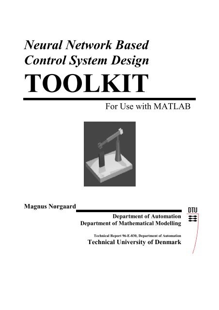
<strong>Neural</strong> <strong>Network</strong> <strong>Based</strong><br />
<strong>Control</strong> <strong>System</strong> <strong>Design</strong><br />
<strong>TOOLKIT</strong><br />
Magnus Nørgaard<br />
For Use with MATLAB �<br />
Department of <strong>Automation</strong><br />
Department of Mathematical Modelling<br />
Technical Report 96-E-830, Department of <strong>Automation</strong><br />
Technical University of Denmark
Release Notes<br />
<strong>Neural</strong> <strong>Network</strong> <strong>Based</strong><br />
<strong>Control</strong> <strong>System</strong> <strong>Design</strong><br />
Toolkit<br />
Version 1.0<br />
Department of <strong>Automation</strong>, Technical University of Denmark, June 20, 1997<br />
This note contains important information on how the present set of tools is to be installed and the<br />
conditions under which it may be used. Please read it carefully before use.<br />
It is important that the NNSYSID toolbox (<strong>Neural</strong> <strong>Network</strong> based SYStem IDentification) has<br />
been installed in advance.<br />
INSTALLING THE <strong>TOOLKIT</strong><br />
° The toolkit is provided in two versions. One for MATLAB 4.2 an one for<br />
MATLAB 5. Both versions have been tested under UNIX on a HP9000/735 and<br />
MATLAB 4.2c.1 for WINDOWS 3.1/95 on an IBM compatible PENTIUM.<br />
° The entire toolkit is implemented as ordinary m-files and thus it should work<br />
equally well on all hardware platforms. However, a fast computer is highly<br />
recommended.<br />
° The Signal Processing toolbox is the only official MathWorks toolbox required by<br />
NNCTRL. However, the <strong>Control</strong> Toolbox is also used in one of the demonstration<br />
programs (“lintest”). Although not a requirement, it is an advantage if SIMULINK<br />
is available as well.
° When properly installed, the structure of the toolkit is as follows:<br />
• NNCTRL<br />
Basic directory containing different Readme-files and the following three<br />
subdirectories:<br />
• CTRLTOOL<br />
The actual toolkit functions and script-files.<br />
• CTRLDEMO<br />
Initialization files, SIMULINK models, and mat-files used for<br />
demonstration.<br />
• TEMPLATE<br />
“Templates” for the initialization files which are called by the<br />
programs in the CTRLTOOL directory.<br />
Your MATLAB path must include the directory CTRLTOOL as well as the<br />
directory containing the NNSYSID toolbox:<br />
>> path(path,’/xx/xx/NNCTRL/CTRLTOOL’)<br />
>> path(path,’/xx/xx/NNSYSID’)<br />
If the tools are going to be used on a regular basis it is recommended that the path<br />
statements are included in ones personal startup.m file (see the MATLABmanual).<br />
During normal use one begins by copying the initialization file associated with the<br />
desired control system from the TEMPLATE directory to the working directory.<br />
The file must then be modified to comply with the application under<br />
consideration. Typical working procedures can be seen by running the<br />
demonstration programs. Furthermore, the different text files found in the<br />
NNCTRL directory provide supplementary information on this matter.<br />
When running the demonstration programs the working directory must be the<br />
directory NNCTRL/CTRLDEMO.<br />
° The checks for incorrect program/function calls are not very thorough and<br />
consequently MATLAB will often respond with quite incomprehensible error<br />
messages when a program or function is incorrectly invoked.<br />
4
CONDITIONS/ DISCLAIMER<br />
By using the toolbox the user agrees to all of the following:<br />
° If one is going to publish any work in which this toolkit has been used, please<br />
remember it was obtained free of charge and include a reference to this technical<br />
report (M. Nørgaard: ”<strong>Neural</strong> <strong>Network</strong> <strong>Based</strong> <strong>Control</strong> <strong>System</strong> <strong>Design</strong> Toolkit,”<br />
Tech. Report. 96-E-830, Department of <strong>Automation</strong>, Technical University of<br />
Denmark, 1996).<br />
° Magnus Nørgaard and the Department of <strong>Automation</strong> do not offer any support for<br />
this product whatsoever. The toolkit is offered free of charge - take it or leave it!<br />
° The toolkit is copyrighted freeware by Magnus Nørgaard/Department of<br />
<strong>Automation</strong>, DTU. It may be distributed freely unmodified. It is, however, not<br />
permitted to utilize any part of the software in commercial products without prior<br />
written consent of Magnus Nørgaard, The Department of <strong>Automation</strong>, DTU.<br />
° THE <strong>TOOLKIT</strong> IS PROVIDED “AS-IS” WITHOUT WARRENTY OF ANY<br />
KIND, EITHER EXPRESS OR IMPLIED, INCLUDING BUT NOT LIMITED<br />
TO THE IMPLIED WARRENTIES OR CONDITIONS OF MECHANTABILITY<br />
OR FITNESS FOR A PARTICULAR PURPOSE. IN NO EVENT SHALL<br />
MAGNUS NØRGAARD AND/OR THE DEPARTMENT OF AUTOMATION<br />
BE LIABLE FOR ANY SPECIAL, INCIDENTAL, INDIRECT, OR<br />
CONSEQUENTIAL DAMAGES OF ANY KIND, OR DAMAGES<br />
WHATSOEVER RESULTING FROM LOSS OF USE, DATA, OR PROFITS,<br />
WHETHER OR NOT MN/IAU HAVE BEEN ADVISED OF THE POSSIBILITY<br />
OF SUCH DAMAGES, AND/OR ON ANY THEORY OF LIABILITY ARISING<br />
OUT OF OR IN CONNECTION WITH THE USE OR PERFORMANCE OF<br />
THIS SOFTWARE.<br />
MATLAB is a trademark of The MathWorks, Inc.<br />
MS-Windows is a trademark of Microsoft Coporation.<br />
Trademarks of other companies and/or organizations mentioned in this documentation appear for<br />
identification purposes only and are the property of their respective companies and/or<br />
organizations.
ACKNOWLEDGEMENTS<br />
The work with these tools was initiated during a stay at the Neuro-Engineering Group, NASA<br />
Ames Research Center. The group members, and in particular their “fearless leader” Dr. Charles<br />
(“Chuck”) Jorgensen, are gratefully acknowledged for creating an inspiring atmosphere. I thank<br />
Niels Kjølstad Poulsen from the Department of Mathematical Modelling for generously letting<br />
me draw on his wealth of knowlegde within most areas of control system design. Also, I wish to<br />
acknowledge Ole Ravn, Paul Haase Sørensen and Elbert Hendricks, Department of <strong>Automation</strong><br />
for their suggestions and comments. In all neural network related matters, Lars Kai Hansen and<br />
the neural network group at the Department of Mathematical Modelling has been a major<br />
inspiration and I wish to thank them too.<br />
June 20, 1997<br />
Magnus Nørgaard<br />
Department of <strong>Automation</strong>, Building 326<br />
Technical University of Denmark<br />
2800 Lyngby<br />
Denmark<br />
e-mail:pmn@iau.dtu.dk<br />
6
1 Tutorial<br />
This manual documents an engineering tool for design and simulation of control systems for processes<br />
that are nonlinear and difficult to model in a deductive fashion. The approach to the problem has been<br />
the typical system identification approach to model based control of an unknown process:<br />
1. <strong>System</strong> identification. I.e., infer a neural network model of the process to be controlled from a set of<br />
data collected in an experiment with the process.<br />
2. <strong>Based</strong> on the identified model one or more controllers are designed (these may be neural networks<br />
as well). Run some simulations to tune the design parameters, and select the controller that appears<br />
to be most suitable for the application.<br />
3. Implementation on a real-time platform and application to real process.<br />
Obviously, in practice the three stages are not necessarily completely independent.<br />
While the NNSYSID toolbox described in Nørgaard (1995) was explicitly designed for solving the<br />
system identification task, the NNCTRL toolkit has been developed to assist the control engineer in<br />
solving the second task. The toolkit is developed in MATLAB due to the excellent data visualization<br />
features and its support for simulation of dynamic systems. In addition, it has been a major motivation<br />
that MATLAB is extremely popular in the control engineering community. Apart from the NNSYSID<br />
toolbox the toolkit requires the Signal Processing toolbox provided by the MathWorks, Inc. Although<br />
not a vital requirement it is also an advantage if SIMULINK � is available. If it is not present,<br />
MATLAB’s built-in ODE solver is used instead.<br />
The NNCTRL toolkit provides concepts where a network is used directly as the controller as well as<br />
indirect designs that are based on a neural network process model. The concepts supported by the<br />
toolkit include: Direct inverse control, internal model control, feedforward control, optimal control,<br />
feedback linearization, nonlinear generalized predictive control, and control based on instantaneous<br />
linearization. The toolkit is primarily intended to be used on time-invariant, single-input-single-output<br />
(SISO) processes.<br />
The NNCTRL toolkit has been given a flexible structure to accommodate incorporation of the user’s<br />
personal neural network architectures and control system designs. Since the entire toolkit has been<br />
implemented as ordinary ‘m-files’ it is very easy to understand and modify the existing code if desired.<br />
This is an attractive feature if the designs provided in advance are not considered sufficient for the<br />
applications under consideration or if the user would like to test new ideas.<br />
First the manual describes the fundamental program structure shared by the different neural network<br />
based control systems and training algorithms. Subsequently an example is given of how the user
1. Tutorial<br />
specifies the design parameters associated with a given application. Finally the different functions in the<br />
toolkit are presented by category in accordance with the type of control system to which they belong.<br />
1.1 THE BASIC FRAMEWORK<br />
All the different control systems have been implemented within the same framework. This framework is<br />
composed of different standard elements such as reading a design parameter file, variable initialization,<br />
generating a reference signal, process simulation, a constant gain PID controller, data storage, data<br />
visualization, and more. The control systems can be divided into two fundamentally different<br />
categories:<br />
1-2<br />
• Direct design: the controller is directly implemented by a neural network.<br />
• Indirect design: The controller is not itself a neural network but it is based on a neural<br />
network model of the process.<br />
The program structure is slightly different for each of the two categories. To illustrate the difference<br />
they are shown in fig. 1 and fig. 2, respectively.<br />
C<br />
B<br />
<strong>Design</strong> parameters<br />
Initializations<br />
Main loop begin<br />
Compute reference<br />
Compute output from process<br />
(Update weights)<br />
Compute control<br />
Time updates<br />
End loop<br />
Plot simulation results<br />
A<br />
Simulink, Matlab<br />
or neural net<br />
model<br />
Figure 1. Program structure for the direct design (i.e., the controller is a neural network). In some<br />
cases it is possible to train the controller on-line and for this reason a step called: “update weights”<br />
has been included.
C<br />
B<br />
<strong>Design</strong> parameters<br />
Initializations<br />
Main loop begin<br />
Compute reference<br />
Compute output from process<br />
<strong>Design</strong> controller<br />
Compute control<br />
Time updates<br />
End loop<br />
Plot simulation results<br />
Simulink, Matlab<br />
or neural net<br />
model<br />
1. Tutorial<br />
Figure 2. Program structure for the indirect design, i.e., when the controller is based on a neural<br />
network model of the process.<br />
Each of the boxes in fig. 1 and fig. 2 specifies a MATLAB script file or function. The three basic<br />
components are:<br />
A) A function describing the process to be controlled. The process can be specified as a SIMULINK<br />
model, a MATLAB function containing the differential equations, or a neural network model of the<br />
process. The Simulink and MATLAB options are of course only relevant when a mathematical<br />
model of the process is available in advance.<br />
B) A MATLAB script file containing design parameters and variables to be initialized by the user. The<br />
initializations that are typically required include: choice of reference signal, sampling frequency,<br />
name of SIMULINK/MATLAB function implementing the process, PID or neural network based<br />
controller, design parameters for the controller. This file has a prespecified name and format that is<br />
associated with the type of control system. The name is always concluded by the letters init.m (e.g.,<br />
invinit.m in direct inverse control and npcinit.m in nonlinear predictive control). A typical NNCTRL<br />
session is initiated by copying a “template” initialization file to the working directory. This file is<br />
then modified to comply with the application under consideration.<br />
C) The main program which automatically reads the initialization file and simulates the process. This<br />
program usually contains the letters con.m in its name to specify that it is the control system<br />
simulation program (for example invcon.m in direct inverse control and optcon.m in optimal<br />
control). It should be emphasized that the program structure does not always follow the patterns<br />
shown in fig. 1 and fig. 2 exactly, but that small variations may occur.<br />
1.2 A TYPICAL INITIALIZATION FILE<br />
During normal operation the user will only need to modify an initialization file containing the basic<br />
design parameters and initializations for the simulation/training. More experienced users may also wish<br />
to modify the actual simulation programs to incorporate their personal algorithms, but this topic is not<br />
covered here. As an example of a typical initialization file, the file used for simulation of nonlinear<br />
predictive control is shown on the following page. Subsequently the different design parameters are<br />
discussed.<br />
NNCTRL Toolkit User’s Guide 1-3<br />
A
1. Tutorial<br />
1-4<br />
% -------------------------------> NPCINIT.M = nb)<br />
Nu = 2; % <strong>Control</strong> horizon<br />
rho = 0.03; % Penalty factor on differenced control signal<br />
% -- Minimization algorithm initialzations -<br />
% maxiter: Maxiumum number of Levenberg-Marquardt/Quasi-Newton iteratons.<br />
% delta : If the 2-norm of the difference to the previous iterate is smaller<br />
% than 'delta', the algorithm is terminated.<br />
% initval: A string which will be evaluated by npccon1/2. To avoid problems with<br />
% local minima, different initial values of the most future component<br />
% of the 'sequence of future controls' can be initialized differenly.<br />
% I.e. the minimization algorithm is executed once for each element<br />
% in 'initval'. Use initval = '[upmin(Nu)]' as default.<br />
maxiter = 5; % Max. number of iterations to determine u<br />
delta = 1e-4; % Norm-of-control-change-stop criterion<br />
initval = '[upmin(Nu)]';<br />
% ----------- Reference signal ------------dc<br />
= 0; % DC-level<br />
sq_amp = 3; % Amplitude of square signals (row vector)<br />
sq_freq = 0.1; % Frequencies of square signals (column vector)<br />
sin_amp = [0]; % Amplitude of sine signals (row vector)<br />
sin_freq= [0]'; % Frequencies of sine signals (column vector)<br />
Nvar = 0'; % Variance of white noise signal<br />
% -- Constant Gain <strong>Control</strong>ler Parameters --<br />
K=8; % PID parameters<br />
Td=0.8; % PID<br />
alf=0.1; % PID<br />
Wi=0.2; % PID (1/Ti)<br />
% ------ Specify data vectors to plot -------<br />
% Notice that all strings in plot_a resp. plot_b must have equal length<br />
plot_a(1,:) = 'ref_data ';<br />
plot_a(2,:) = 'y_data ';<br />
plot_b(1,:) = 'u_data';
% ---------- Switches ----------regty<br />
='npc'; % <strong>Control</strong>ler type (npc, pid, none)<br />
refty ='siggener'; % Reference signal(siggener/)<br />
simul ='simulink'; % <strong>Control</strong> object spec.(simulink/matlab/nnet)<br />
1. Tutorial<br />
regty defines the type of controller. It is possible to make a complete open-loop simulation (‘none’),<br />
to use a constant gain PID-controller (‘pid’) or, in this case, a generalized predictive control design<br />
based on a neural network predictor for the process (‘npc’).<br />
refty defines the type of reference trajectory. It is possible to use a signal generator (‘siggener’)<br />
which can produce square waves, sinusoidals and white noise. Alternatively one can specify the name<br />
of a vector containing the desired reference trajectory (for example, refty=‘myref’). If the latter<br />
option is used, the vector must exist in the workspace or be defined elsewhere in the initialization file.<br />
simul specifies the “tool” used for modelling the process. There are three possibilities: a SIMULINK<br />
model (‘simulink’), a MATLAB model (‘matlab’), or a neural network model (‘nnet’).<br />
% ---------- Initializations -----------<br />
Ts = 0.2; % Sampling period (in seconds)<br />
samples = 300; % Number of samples in simulation<br />
Ts is the sampling period in seconds and samples specifies the the number of samples to be simulated.<br />
% -- <strong>System</strong> to be <strong>Control</strong>led (SIMULINK) -sim_model<br />
= 'spm1'; % Name of SIMULINK model<br />
If simul=‘simulink’ the program will simulate the “process” specified in a SIMULINK diagram with<br />
the name defined in sim_model. The SIMULINK block must have an inport specifying the input and<br />
an outport specifying the output, but apart from this there are no constraints on how the model is built.<br />
The picture below shows the SIMULINK model used in the demos:<br />
1<br />
Inport<br />
+<br />
−<br />
Sum<br />
.<br />
x2<br />
1<br />
s<br />
Integrator1<br />
.<br />
x2=x1<br />
1<br />
s<br />
y=x1<br />
NNCTRL Toolkit User’s Guide 1-5<br />
*<br />
Product<br />
Integrator2<br />
1<br />
Outport
1. Tutorial<br />
% --- <strong>System</strong> to be <strong>Control</strong>led (MATLAB) -mat_model<br />
= 'springm'; % Name of MATLAB model<br />
model_out = 'smout'; % Output equation (function of the states)<br />
x0 = [0;0]; % Initial states<br />
If simul=‘matlab’ the program will simulate the “process” defined by the two MATLAB files defined<br />
in mat_model (the differential equations) and model_out (the output as a function of the states).<br />
For example:<br />
function xdot=springm(t,x)<br />
global ugl;<br />
xdot = [x(2) ; -x(1)-x(2)-x(1)*x(1)*x(1)+ugl];<br />
and:<br />
function y=smout(x);<br />
y = x(1);<br />
x0 is a vector specifying the initial states.<br />
It is important to include the global ugl; statement (ugl is short for “u global”) in the MATLAB<br />
function containing the differential equations describing the model. This is to comply with the format<br />
required for passing the control signal to a function called by MATLAB’s differential equation solver<br />
ode45.<br />
% ----- <strong>Neural</strong> <strong>Network</strong> Specification ------<br />
% "nnfile" must contain the following variables which together define<br />
% an NNARX model:<br />
% NN, NetDef, W1, W2<br />
% (i.e. regressor structure, architecture definition, and weight matrices)<br />
nnfile = 'forward'; % Name of file containing the neural network model<br />
The predictive controller requires a neural network model to predict the future outputs. This network<br />
must be a NNARX (or NNOE) model created with the NNSYSID-toolbox. Regressor structure (NN),<br />
network architecture (NetDef) and weight matrices (W1 and W2) must be saved in a file. The name of<br />
the file name must be specified in the variable nnfile. If neither a SIMULINK model nor a MATLAB<br />
model of the process exists, the network model can also be used for simulating the process.<br />
Latest Breaking News: NNCTRL for MATLAB 5/SIMULINK 2:<br />
New ordinary differential equation (ODE) solvers are supplied with MATLAB5/SIMULINK 2 and the<br />
call of these solvers from within MATLAB has been changed. If a SIMULINK function of the process<br />
is available, the additional variable ?? must be specified. This variable must contain the name of the<br />
ODE solver.<br />
% -- <strong>System</strong> to be <strong>Control</strong>led (SIMULINK) -integrator<br />
= 'ode45'; % Name of dif. eq. solver (f. ex. ode45 or ode15s)<br />
sim_model = 'spm1'; % Name of SIMULINK model<br />
The reader is referred to the MATLAB manuals for more details on the different ODE solvers.<br />
1-6
1. Tutorial<br />
If a model of the process is available only in MATLAB, the solver ‘ode45’ has been preselected. If the<br />
user prefers another ODE solver the name of this should be inserted in the main program.<br />
% ------------ Reference filter ---------------<br />
Am = [1.0 -0.7]; % Denominator of filter<br />
Bm = [0.3]; % Numerator of filter<br />
It is possible to filter the reference trajectory if desired. The filter’s transfer function is specified in the<br />
polynomials A m and B m. The specified choice corresponds to:<br />
0. 3<br />
r( t)<br />
= r( t)<br />
−<br />
1− 0. 7q 1<br />
% ---------- GPC initializations -----------<br />
N1 = 1; % Min. prediction horizon (must equal the time delay!)<br />
N2 = 7; % Max. prediction horizon (>= nb)<br />
Nu = 2; % <strong>Control</strong> horizon<br />
rho = 0.03; % Penalty factor on differenced control signal<br />
%-- Minimization algorithm initialzations -<br />
%maxiter: Maxiumum number of Levenberg-Marquardt/Quasi-Newton iteratons.<br />
%delta : If the 2-norm of the difference to the previous iterate is smaller<br />
% than 'delta', the algorithm is terminated.<br />
%initval: A string which will be evaluated by npccon1/2. To avoid problems with<br />
% local minima, different initial values of the most future component<br />
% of the 'sequence of future controls' can be initialized differenly.<br />
% I.e. the minimization algorithm is executed once for each element<br />
% in 'initval'. Use initval = '[upmin(Nu)]' as default.<br />
maxiter = 5; % Max. number of iterations to determine u<br />
delta = 1e-4; % Norm-of-control-change-stop criterion<br />
initval = '[upmin(Nu)]';<br />
If the nonlinear generalized predictive control strategy has been selected by setting regty=‘npc’ the<br />
design parameters must be specified in N 1, N 2, N u, and rho:<br />
J ( t,<br />
U ( t))<br />
=<br />
5<br />
N<br />
2<br />
2<br />
∑[<br />
r(<br />
t + i)<br />
− yˆ<br />
( t + i)<br />
] + ρ∑<br />
[ Δu(<br />
t + i −1)<br />
]<br />
i=<br />
N1<br />
The GPC-criterion can be minimized using two different schemes: a Quasi-Newton algorithm (obtained<br />
by running the program npccon1) or a Levenberg-Marquardt algorithm (obtained by running npccon2).<br />
maxiter specifies the maximum number of iterations and delta defines the stopping criterion. The<br />
criterion may have several local minima and consequently it may be desireable to specify different<br />
starting points for the minimization algorithm. This can be done in the vector initval.<br />
NNCTRL Toolkit User’s Guide 1-7<br />
Nu<br />
i=<br />
1<br />
2
1. Tutorial<br />
% ----------- Reference signal ------------dc<br />
= 0; % DC-level<br />
sq_amp = [3]; % Amplitude of square signals (row vector)<br />
sq_freq = [0.1]’; % Frequencies of square signals (column vector)<br />
sin_amp = [0]; % Amplitude of sine signals (row vector)<br />
sin_freq= [0]'; % Frequencies of sine signals (column vector)<br />
Nvar = 0'; % Variance of white noise signal<br />
If refty=‘siggener’ a simple signal generator is invoked to generate the reference trajectory. The<br />
variables above define the trajectory. It is possible to create a trajectory composed of several square<br />
waves and/or sinusoidals by defining sq_amp, sq_freq, sin_amp, and sin_freq as vectors.<br />
% -- Constant Gain <strong>Control</strong>ler Parameters --<br />
K=8; % PID parameters<br />
Td=0.8; % PID<br />
alf=0.1; % PID<br />
Wi=0.2; % PID (1/Ti)<br />
It is possible to use an ordinary PID controller instead of the predictive controller. This is achieved by<br />
setting regty=‘pid’. The controller is implemented as a discrete version of:<br />
1-8<br />
1+<br />
Td s 1+<br />
Tis D( s) = K<br />
1+<br />
alf * T s T s<br />
% ------ Specify data vectors to plot -------<br />
% Notice that all strings in plot_a resp. plot_b must have equal length<br />
plot_a(1,:) = 'ref_data';<br />
plot_a(2,:) = 'y_data ';<br />
plot_b(1,:) = 'u_data';<br />
Finally it is possibly to specify the signals to be plotted. The signals considered most interesting are<br />
stored in vectors with names concluded by the letters ‘_data’. For example, ref_data specifies the<br />
reference, y_data the output signal and u_data the control signal. plot_a and plot_b are matrices of<br />
strings which are evaluated by the program. For example, it is possible to write:<br />
plot_b(1,:) = '3.5*u_data+10';<br />
to plot a scaled version of the control signal. Since the control system simulation programs are scriptfiles,<br />
all parameters, vectors, and matrices will be available in the workspace when the simulation is<br />
completed and they can be used in further analyses. A typical plot produced by the simulation program<br />
is shown below.<br />
d<br />
i
3<br />
2<br />
1<br />
0<br />
−1<br />
−2<br />
Nonlinear Predictive <strong>Control</strong><br />
1. Tutorial<br />
NNCTRL Toolkit User’s Guide 1-9<br />
ref_data<br />
y_data<br />
−3<br />
0 50 100 150<br />
Samples<br />
200 250<br />
15<br />
10<br />
5<br />
0<br />
−5<br />
−10<br />
u_data<br />
−15<br />
0 50 100 150<br />
Samples<br />
200 250
2 <strong>Control</strong> system design<br />
In this chapter the control systems implemented in the NNCTRL toolkit are introduced. The control<br />
systems provided are: direct inverse control, internal model control, feedforward, control by inputoutput<br />
linearization, optimal control, approximate pole placement control, minimum variance control,<br />
predictive control based on instantaneous linearization, and nonlinear predictive control.<br />
To experience the features of the different types of neural network based control it is often relevant to<br />
investigate how the controllers perform on a well-known process. In fact, this is one of the primary<br />
purposes of this toolkit. For this reason it is possible to control models that are built in SIMULINK � or<br />
differential equation models that are specified in MATLAB � . Also it is possible to simulate an<br />
experiment with the process to acquire a set of data for system identification and controller design.<br />
In the following sections the different functions are discussed, starting with how to simulate an<br />
experiment (if externally generated data are used, one can skip this section). Not all the options for the<br />
different *init.m files will be discussed since they have a great deal of overlap with one another and<br />
with the one shown in the previous chapter.<br />
2.1 SIMULATING THE EXPERIMENT<br />
experim<br />
expinit<br />
Experiment Simulation<br />
Simulate experiment.<br />
File with design parameters for experim.<br />
If the NNCTRL toolkit is used to gain experience with neural network based control or if a<br />
rudimentary model of the process to be controlled exists, the experiment can be simulated using a<br />
SIMULINK � or MATLAB � model of the process. The experiment can be conducted in open-loop, but<br />
if the process is poorly damped or unstable it is also possible to make the experiment in closed-loop<br />
with a PID-controller (or an RST-controller).
2. <strong>Control</strong> <strong>System</strong> <strong>Design</strong><br />
2-2<br />
r<br />
+<br />
-<br />
up<br />
+<br />
+<br />
PID controller <strong>System</strong><br />
u<br />
uc<br />
Figure 3 Collecting data in closed-loop with a PID-controller.<br />
A manually tuned PID-controller will often be designed somewhat conservatively - its primary<br />
objective is to stabilize the process. It is therefore possible to add a signal (up) directly to the control<br />
signal to ensure a certain high frequency content in the data set. If the experiment is conducted in openloop<br />
it makes no difference whether r or up is used as the reference signal.<br />
The function experim simulates the experiment and the file expinit contains the initializations to be<br />
specified by the user. Some excerpts from the expinit file are given below:<br />
% ---------- Switches ----------regty<br />
='none'; % <strong>Control</strong>ler type (rst, pid, none)<br />
refty ='predef'; % Reference signal (siggener/none/)<br />
probety ='none'; % Probing signal (none/)<br />
regty specifies the type of controller. regty=‘none’ implies that the experiment is conducted in openloop,<br />
regty=‘pid’ that the experiment is conducted in closed-loop with a PID-controller, and<br />
regty=‘rst’ that the experiment is conducted in closed-loop with an RST-controller. The design<br />
parameters of the PID and RST controllers are also set in the file:<br />
% -------- Linear <strong>Control</strong>ler Parameters ---------<br />
K=8; % PID parameters<br />
Td=0.8; % PID<br />
alf=0.1; % PID<br />
Wi=0.2; % PID (1/Ti)<br />
r0=0.0609; % RST parameters<br />
r1=0.0514; % RST<br />
t0=0.2; % RST<br />
s0=0.802; % RST<br />
s1=-0.602; % RST<br />
R = [r0 r1];<br />
S = [s0 s1];<br />
T = t0;<br />
refty selects the type of reference signal (r) and probety the type of signal added directly to the<br />
control signal in a closed-loop experiment (up). If refty=‘siggener’ the built-in signal generator is<br />
used. If this is not adequate it is possible to use a signal defined in a vector which is available in the<br />
workspace. If the name of the vector is my_signal then set refty= ‘my_signal’.<br />
y
2.2 CONTROL WITH INVERSE MODELS<br />
general<br />
special1<br />
invinit1<br />
special2<br />
special3<br />
invinit2<br />
invsim<br />
invcon<br />
invinit<br />
imccon<br />
imcinit<br />
ffcon<br />
ffinit<br />
invtest<br />
<strong>Control</strong> with Inverse Models<br />
General training of inverse models.<br />
Specialized back-prop training of inverse models.<br />
File with design parameters for special1.<br />
Specialized training with an RPLR type Gauss-Newton method.<br />
Specialized training with an RPEM type Gauss-Newton method.<br />
File with design parameters for special2 and special3.<br />
Function for evaluating inverse models.<br />
Program for simulating direct inverse control.<br />
File with design parameters for invcon.<br />
Program for simulating internal model control.<br />
File with design parameters for imccon.<br />
Program for simulating process with feedforward control.<br />
File with design parameters for ffcon.<br />
Program for demonstrating direct inverse control.<br />
2. <strong>Control</strong> <strong>System</strong> <strong>Design</strong><br />
Conceptually, the most fundamental neural network based controllers are probably those using the<br />
“inverse” of the process as the controller. The most simple concept is called direct inverse control. The<br />
principle of this is that if the process can be described by:<br />
a network is trained as the inverse of the process:<br />
( )<br />
y( t + 1) = g y( t), , y( t − n + 1),<br />
u( t), , u( t − m)<br />
( ( 1), ( ), , ( 1), ( 1),<br />
( ) )<br />
¡ ¡ −1<br />
u( t) = g y t + y t y t − n + u t − u t − m<br />
¢<br />
The inverse model is subsequently applied as the controller for the proces by inserting the desired<br />
output, the reference r(t+1), instead of the output y(t+1). There are several references available which<br />
use this idea, e.g., Psaltis et al. (1988), Hunt & Sbarbaro (1991), and Hunt et al. (1992). See also fig. 4.<br />
Internal model control (IMC) and feedforward control represent other strategies that utilize inverse<br />
models.<br />
NNCTRL Toolkit User’s Guide 2-3
2. <strong>Control</strong> <strong>System</strong> <strong>Design</strong><br />
2-4<br />
r(t+1)<br />
q -1<br />
q -2<br />
q -2<br />
NN<br />
inverse<br />
model<br />
u(t)<br />
Figure 4 Direct inverse control.<br />
Process<br />
y(t+1)<br />
Before considering the actual control system, an inverse model must be trained. Two strategies for<br />
obtaining the inverse model are provided in the toolkit: generalized training and specialized training<br />
(Psaltis et al. 1988). In generalized training a network is trained off-line to minimize the following<br />
criterion (θ specifies the weights in the network):<br />
N<br />
£<br />
( ( ) )<br />
J ( θ ) = u( t) − u t<br />
1<br />
∑<br />
t=<br />
1<br />
An experiment is performed and a set of corresponding inputs and outputs are stored. Subsequently the<br />
function general, which applies a version of the Levenberg-Marquardt method (Fletcher, 1987), is<br />
invoked.<br />
Specialized training is an on-line procedure related to model-reference adaptive control. The idea is to<br />
minimize the criterion:<br />
where<br />
∑(<br />
m )<br />
J ( θ ) = y ( t) − y( t)<br />
2<br />
t<br />
−1<br />
q Bm ( q)<br />
ym ( t)<br />
= r( t)<br />
A ( q)<br />
The inverse model is obtained if Am=Bm=1, but often a low-pass filtered version is preferred. In this<br />
case the result will be some kind of “detuned” (or “smoothed”) inverse model.<br />
Specialized training is often said to be goal directed because it, as opposed to generalized training,<br />
attempts to train the network so that the output of the process follows the reference closely. For this<br />
reason, specialized training is particularly well-suited for optimizing the controller for a prescribed<br />
reference trajectory. This is a relevant feature in many robotics applications. Also it is with special<br />
training possible to make an inverse model for processes that are not one-to-one.<br />
Specialized training must be performed on-line and thus it is much more difficult to carry out in<br />
practice than generalized training. Before the actual training of the inverse model is initiated, a<br />
“forward” model of the process must be trained since this is required by the scheme. This can be<br />
m<br />
2<br />
2
2. <strong>Control</strong> <strong>System</strong> <strong>Design</strong><br />
created with the NNSYSID toolbox from a data set collected in an experiment performed in advance as<br />
described in section 2.1. The principle is depicted in fig. 5.<br />
e u<br />
r NN<br />
inverse model<br />
Reference<br />
model<br />
u<br />
NN<br />
forward model<br />
Process<br />
Figure 5 The principle of specialized training.<br />
Unlike generalized training the controller design is model based when the specialized training scheme is<br />
applied since a model of the process is required. Details on the principle can be found in Hunt &<br />
Sbarbaro (1991). Three different variations of the scheme have been implemented: One using a<br />
recursive back-propagation algorithm for minimizing the criterion (special1) and two more rapid<br />
methods using different variations of the recursive Gauss-Newton algorithm (special2 and special3).<br />
Specialized training is more complex to implement than generalized training and requires more design<br />
parameters. For this reason it has not been implemented as MATLAB functions like generalized<br />
training. The three variations of the scheme are instead implemented by the same type of combination<br />
of script files and initialization files as was discussed in chapter 1.<br />
The difference between special 1 and special2 on one side and special3 on the other side lies in the<br />
way the derivative of the process output with respect to the weights of the inverse model is<br />
approximated. special 1 and special2 have been implemented in the spirit of recursive “pseudo-linear<br />
regression” methods (Ljung, 1987) in the sense that the past outputs and past controls dependency on<br />
the network weights is disregarded:<br />
¤<br />
dy( t)<br />
∂y(<br />
t)<br />
du( t −1)<br />
∂y(<br />
t)<br />
∂u(<br />
t −1)<br />
ψ ( t)<br />
= =<br />
≈<br />
dθ<br />
∂u( t −1)<br />
dθ<br />
∂u(<br />
t −1)<br />
∂θ<br />
special3 is closer to the true recursive prediction error method discussed in Ljung (1987):<br />
dy( t)<br />
∂y(<br />
t)<br />
du( t −1)<br />
ψ ( t)<br />
= =<br />
dθ<br />
∂u( t −1)<br />
dθ<br />
¤ ¤ n<br />
m<br />
∂y(<br />
t)<br />
⎡∂u(<br />
t −1)<br />
∂u(<br />
t −1)<br />
dy( t − i)<br />
∂u(<br />
t −1)<br />
du( t − i)<br />
⎤<br />
≈<br />
∂u(<br />
t − )<br />
⎢ + ∑ + ∑<br />
1 ⎣ ∂θ i ∂y( t − i)<br />
dθ<br />
i ∂u( t − i)<br />
dθ<br />
⎥<br />
= 1 = 2<br />
⎦<br />
In special2 and special3 the user can choose one of three updating formulas (see Åström &<br />
Wittenmark, 1995; Salgado et al, 1988):<br />
NNCTRL Toolkit User’s Guide 2-5<br />
ym<br />
e<br />
y<br />
y^<br />
-<br />
+
2. <strong>Control</strong> <strong>System</strong> <strong>Design</strong><br />
Exponential forgetting (method=‘ff’):<br />
2-6<br />
T ( )<br />
K( t) = P( t − 1) ψ ( t) λI + ψ ( t) P( t − 1)<br />
ψ ( t)<br />
¥<br />
( ( ) )<br />
¥ ¥<br />
θ( t) = θ(<br />
t − 1)<br />
+ K( t) y( t) − y t<br />
T<br />
( 1 ψ 1 )<br />
P( t) = P( t − ) − K( t) ( t) P( t − )<br />
Constant-trace (method=‘ct’):<br />
λ<br />
T ( )<br />
K( t) = P( t − 1) ψ ( t) λ + ψ ( t) P( t − 1)<br />
ψ ( t)<br />
¥<br />
( ( ) )<br />
¥ ¥<br />
θ( t) = θ(<br />
t − 1)<br />
+ K( t) y( t) − y t<br />
−1<br />
−1<br />
T<br />
⎛ P( t − 1) ψ ( t) ψ ( t) P( t − 1)<br />
⎞<br />
P( t) = ⎜ P( t − 1)<br />
+<br />
T<br />
⎟<br />
⎝<br />
1 + ψ ( t) P( t − 1)<br />
ψ ( t)<br />
⎠<br />
α − α<br />
P( t)<br />
=<br />
tr( P( t))<br />
max min<br />
P( t) + α I<br />
min<br />
Exponential Forgetting and Resetting Algorithm (method=‘efra’):<br />
T ( )<br />
K( t) = αP( t − 1) ψ ( t) 1 + ψ ( t) P( t − 1)<br />
ψ ( t)<br />
¥<br />
( ( ) )<br />
¥ ¥<br />
θ( t) = θ(<br />
t − 1)<br />
+ K( t) y( t) − y t<br />
1<br />
T<br />
2<br />
P( t) = P( t − 1) − K( t) ψ ( t) P( t − 1) + βI − δP<br />
( t − 1)<br />
λ<br />
−1<br />
−1<br />
λ<br />
To illustrate how specialized training is executed, some excerpts from the file invinit2 are shown<br />
below. This file contains the design parameters for both special2 and special3. The file invinit1, which<br />
contains the design parameters for special1, has almost the same structure.<br />
% ---------- Switches ----------simul<br />
= 'simulink'; % <strong>System</strong> specification (simulink/matlab/nnet)<br />
method = 'ff'; % Training algorithm (ff/ct/efra)<br />
refty = 'siggener'; % Reference signal (siggener/)<br />
% ------ General Initializations -------<br />
Ts = 0.20; % Sampling period (in seconds)<br />
samples = 200 ; % Number of samples in each epoch
2. <strong>Control</strong> <strong>System</strong> <strong>Design</strong><br />
method specifies the training algorithm. The forgetting factor algorithm will usually give the most rapid<br />
convergence, but be aware of the possibility of covariance blow-up (Åström & Wittenmark, 1995).<br />
refty specifies the type of reference signal.<br />
% ----- <strong>Neural</strong> <strong>Network</strong> Specification ------<br />
%The "forward model file" must contain the following variables which together<br />
% define a NNARX-model:<br />
% NN, NetDeff, W1f, W2f<br />
% and the "inverse model file" must contain<br />
% NN, NetDefi, W1i, W2i<br />
% (i.e. regressor structure, architecture definition, and weight matrices)<br />
nnforw = 'forward'; % Name of file containing forward model<br />
nninv = 'inverse'; % Name of file containing inverse model<br />
nnforw should be set to the name of the file containing the architecture definition and weight matrices<br />
for a neural network model of the process to be controlled. This model is required to provide estimates<br />
of the process’ Jacobian: ∂<br />
¦<br />
y( t)<br />
∂u(<br />
t −1)<br />
nninv should be set to the name of a file containing the architecture definition and the initial weight<br />
matrices for the inverse neural network model. The weights can be initialized by random, but most<br />
often it is better to make a rough initialization using generalized training. When working in this way,<br />
specialized training can be considered a fine-tuning of the inverse model.<br />
% ------------ Reference Model ---------------<br />
Am = [1 0.7]; % Model denominator<br />
Bm = [0.3]; % Model numerator<br />
When the ordinary inverse model is needed Am=1 and Bm=1. However, often it is preferred that the<br />
closed-loop system follows a prescribed transfer function model. Am and Bm are then be set to the<br />
desired closed-loop denominator and numerator, respectively.<br />
% ------------ Training parameters ----------maxiter<br />
= 8;<br />
maxiter specifies the number of times that the reference trajectory (of the length specified in the<br />
variable samples) is repeated. The total number of times that the weights are updated are thus<br />
maxiter*samples.<br />
NNCTRL Toolkit User’s Guide 2-7
2. <strong>Control</strong> <strong>System</strong> <strong>Design</strong><br />
% --- Forgetting factor algorithm (ff) ---<br />
% trparms = [lambda p0]<br />
% lambda = forgetting factor (suggested value 0.995)<br />
% p0 = Covariance matrix diagonal (1-10)<br />
%<br />
% --- Constant trace algorithm (ct) ---<br />
% trparms = [lambda alpha_max alpha_min]<br />
% lambda = forgetting factor (suggested value 0.995)<br />
% alpha_max = Max. eigenvalue of covariance matrix (100)<br />
% alpha_min = Min. eigenvaule of covariance matrix (0.001)<br />
%<br />
% --- Exponential Forgetting and Restting Algorithm (efra) ---<br />
% trparms = [alpha beta delta lambda]<br />
% Suggested values:<br />
% alpha = 0.5-1<br />
% beta = 0.001<br />
% delta = 0.001<br />
% lambda = 0.98<br />
trparms = [0.995 10];<br />
%trparms = [0.995 100 0.001];<br />
%trparms = [1 0.001 0.001 0.98];<br />
trparms is a vector containing the design parameters for the update of the covariance matrix in the<br />
recursive Gauss-Newton algorithm. The content of this vector depends of course on the selected<br />
updating scheme (exponential forgetting, constant trace, EFRA).<br />
% ------ Specify data vectors to plot -------<br />
% Notice that all strings in plot_a resp. plot_b must have equal length<br />
plot_a(1,:) = 'ref_data ';<br />
plot_a(2,:) = 'y_data ';<br />
plot_a(3,:) = 'yhat_data';<br />
plot_b(1,:) = 'u_data';<br />
Each time the reference trajectory has been applied once, a plot will appear on the screen with the<br />
signals defined in plot_a and plot_b. The SSE (sum-of-squared-errors) for the error between<br />
reference and output signal is written in the plot to give the user an indication of how the algorithms is<br />
converging.<br />
Once an inverse model has been trained there are different ways in which it can be used for control.<br />
The toolkit provides three different concepts:<br />
Direct inverse control:<br />
As the name indicates the inverse model is directly used as the controller:<br />
The principle was shown in fig. 4.<br />
2-8<br />
¨ ( ( 1), ( ), , ( 1), ( 1),<br />
( ) )<br />
§ −1<br />
u( t) = g r t + y t y t − n + u t − u t − m
2. <strong>Control</strong> <strong>System</strong> <strong>Design</strong><br />
invcon is used for simulating the closed-loop system while the design parameters are specified in the<br />
file invinit. Some examples of design parameters to be initialized in invinit are shown below:<br />
% ---------- Switches ----------regty<br />
='dic'; % <strong>Control</strong>ler type (dic, pid, none)<br />
simul ='simulink’; % <strong>Control</strong> object spec. (simulink/matlab/nnet)<br />
regty=‘dic’ means direct inverse control. If regty=‘pid’ an ordinary PID-controller will be used<br />
instead.<br />
% ----- Inverse <strong>Network</strong> Specification ------<br />
% The file must contain the variables:<br />
% NN, NetDefi, W1i, W2i<br />
% (i.e. regressor structure, architecture definition, and weight matrices)<br />
nninv = 'inverse'; % Name of file<br />
The variable nninv is set to the name of the file containing the regressor structure, architecture<br />
definition and weight matrices for the neural network that is modelling the inverse of the process.<br />
% ------------ Reference Filter ---------------<br />
Am = [1]; % Filter denominator<br />
Bm = [1]; % Filter numerator<br />
Am and Bm defines a filter that is used on the reference signal before it is applied to the inverse model. It<br />
has nothing to do with the reference model used in specialized training. An option to filter the<br />
reference is provided to avoid that the reference signal has a large high frequency component.<br />
Internal model control:<br />
This design has been treated in Hunt & Sbarbaro (1991). The control signal is synthesized by a<br />
combination of a “forward” model of the process and an inverse model. An attractive property of this<br />
design is that it provides an off-set free response regardless of whether or not the process is affected by<br />
a constant disturbance. The scheme is implemented in imccon and imcinit.<br />
d(t)<br />
r(t) Filter NN-controller<br />
+<br />
-<br />
��<br />
��<br />
NN-model<br />
q -1 ©©<br />
NNCTRL Toolkit User’s Guide 2-9<br />
u(t)<br />
Figure 6 Inverse model control (IMC).<br />
Process<br />
q -1 ��<br />
The file imcinit is very similar to invinit. The differences are shown below:<br />
+<br />
y(t)<br />
^<br />
-<br />
y(t)<br />
+
2. <strong>Control</strong> <strong>System</strong> <strong>Design</strong><br />
% ---------- Switches ----------regty<br />
='imc'; % <strong>Control</strong>ler type (imc, pid, none)<br />
regty must be set to 'imc' to select internal model control.<br />
% ----- Inverse <strong>Network</strong> Specification ------<br />
% The file must contain the variables:<br />
% NN, NetDefi, W1i, W2i<br />
% (i.e. regressor structure, architecture definition, and weight matrices)<br />
nninv = 'inverse3'; % File name<br />
% ----- Forward <strong>Network</strong> Specification ------<br />
% The file must contain: NN, NetDeff, W1f, W2f<br />
nnforw = 'forward'; % File name<br />
A neural network model of the process is integrated in the controller design as shown on fig. 6. If the<br />
specialized training scheme was used for creating the inverse model, a model of the process is already<br />
available. Otherwise a new model must be trained before the IMC concept can be used.<br />
% ---------------- Filter ------------------<br />
Am = [1 -0.7]; % Filter denominator<br />
Bm = [0.3]; % Filter numerator<br />
Am and Bm are denominator and numerator of the filter, F, shown in fig.6.<br />
Feedforward<br />
Using inverse models for feedback control leads to a dead-beat type of control which is unsuitable in<br />
many cases. If a PID controller has already been tuned for stabilizing the process, an inverse model can<br />
be used for providing a feedforward signal directly from the reference. This has been proposed in<br />
Leunen (1993) and Sørensen (1994). The scheme is implemented in ffcon and ffinit.<br />
2-10<br />
r<br />
+<br />
-<br />
NN<br />
inverse model<br />
+<br />
+<br />
PID controller Process<br />
u<br />
u fb<br />
Figure 7 Feedforward for optimization of an existing control system.<br />
u ff<br />
y
An excerpt from the file ffinit is shown below:<br />
% ---------- Switches ----------regty<br />
='pidff'; % <strong>Control</strong>ler type (pid, pidff, ff, none)<br />
% -------- Linear <strong>Control</strong>ler Parameters ---------<br />
K=8; % PID parameters<br />
Td=0.8; % PID<br />
alf=0.1; % PID<br />
Wi=0.2; % PID (1/Ti)<br />
2. <strong>Control</strong> <strong>System</strong> <strong>Design</strong><br />
If regty=‘pid’ a constant gain PID controller is used with the parameters defined by K, Td, alf, and<br />
Wi. If regty=‘ff’ the process is controlled in open-loop using the inverse neural network model as a<br />
feedforward controller. regty=‘pidff’ combines the two so that the PID controller is used for<br />
stabilizing the process and suppressing disturbances while the feedforward is used for providing a fast<br />
tracking of the reference.<br />
NNCTRL Toolkit User’s Guide 2-11
2. <strong>Control</strong> <strong>System</strong> <strong>Design</strong><br />
2.3 FEEDBACK LINEARIZATION<br />
2-12<br />
fblcon<br />
fblinit<br />
fbltest<br />
<strong>Control</strong> by Feedback Linearization<br />
Simulate control by feedback linearization.<br />
File with design parameters for fblcon.<br />
Program for demonstrating control by feedback linearization.<br />
Feedback linearization is a common method for controlling certain classes of nonlinear processes. The<br />
toolkit provides a simple example of a discrete input-output linearizing controller that is based on a<br />
neural network model of the process. The NNSYSID toolbox contains the function nniol to train a<br />
neural network model that has the following structure:<br />
� �<br />
( 1 2 )<br />
( )<br />
�<br />
y( t) = f y( t − ), , y( t − n), u( t − ), , u( t − m)<br />
+<br />
g y( t −1), , y( t − n), u( t − 2), , u( t − m) u( t −1)<br />
� �<br />
f and g are two separate networks. A feedback linearizing controller is obtained by calculating the<br />
controls according to:<br />
� �<br />
� �<br />
− ( − + 1 − 1 − + 1 )<br />
( ( ), , ( − + 1), ( − 1), , ( − + 1)<br />
)<br />
w( t) f y( t), , y( t n ), u( t ), , u( t m )<br />
u( t)<br />
=<br />
g y t y t n u t u t m<br />
Selecting the virtual control, w(t), as an appropriate linear combination of past outputs plus the<br />
reference enables an arbitrary assignment of the closed-loop poles. As for the model-reference<br />
controller, feedback linearization is thus a nonlinear counterpart to pole placement with all zeros<br />
canceled (see Åström & Wittenmark, 1995). The principle is depicted in Figure 8.<br />
r(t)<br />
w(t)-f(•)<br />
g(•)<br />
q -2 q -1<br />
u(t-1)<br />
q -1<br />
q -2 q -1<br />
NN-2<br />
g(•)<br />
Process<br />
Figure 8 Discrete feedback linearization.<br />
q -1<br />
q -2 q -1<br />
NN-1<br />
f(•)<br />
y(t)
2. <strong>Control</strong> <strong>System</strong> <strong>Design</strong><br />
The design parameters must be specified in the file fblinit. An excerpt from the file is discussed below.<br />
% ---------- Switches ----------regty<br />
='fbl'; % <strong>Control</strong>ler type (fbl, pid, none)<br />
regty=‘fbl’ gives control by feedback linearization.<br />
% ----- <strong>Neural</strong> <strong>Network</strong> Specification ------<br />
% "nnfile" must contain the following variables which together define<br />
% the network model:<br />
% NN, NetDeff, NetDefg, W1f, W2f, W1g, W2g<br />
% (i.e. regressor structure, architecture definitions, and weight matrices)<br />
nnfile = 'net_file'; % Name of file<br />
nnfile, which contains the regressor structure, architecture definition and weights of the neural<br />
network, must in this case include seven different variables due to the somewhat special network<br />
architecture. NN specifies the regressors and is set as for an NNARX model. NetDeff defines the<br />
architecture of the network implementing f while NetDefg defines the architecture of the network<br />
implementing g. W1f and W2f contain the weights for f while W1g and W2g contain the weights for g.<br />
% ---- Desired characteristic polynomial ---<br />
Am = [1 -1.4 0.49]; % Characteristic polynomial<br />
Am contains the desired closed-loop characteristic polynomial. In this case the polynomial has been<br />
2<br />
selected to Am ( z) = z − 1.4 z + 0 .49 corresponding to two poles in z = 0. 7 .<br />
NNCTRL Toolkit User’s Guide 2-13
2. <strong>Control</strong> <strong>System</strong> <strong>Design</strong><br />
2.4 OPTIMAL CONTROL<br />
2-14<br />
opttrain<br />
optinit<br />
optcon<br />
optinit<br />
opttest<br />
Optimal <strong>Control</strong><br />
Simulate control by feedback linearization.<br />
File with design parameters for opttrain.<br />
Simulate optimal control of process (similar to invcon).<br />
File with design parameters for optcon.<br />
Program for demonstrating the optimal control concept.<br />
A simple training algorithm for design of optimal controllers has been implemented by a small<br />
modification of the specialized training algorithm implemented in special2. The modification consists of<br />
an additional term which is added to the criterion to penalize the squared controls:<br />
( ) ( )<br />
J ( θ) = r( t) − y( t) + ρ u( t)<br />
, ρ ≥ 0<br />
3<br />
∑<br />
t<br />
2 2<br />
The training of the network is very similar to specialized training of inverse models and is also<br />
performed on-line. As for specialized training a “forward” model of the process must have been<br />
identified with the NNSYSID toolbox in advance.<br />
The training is carried out with opttrain which implements a modified recursive Gauss-Newton<br />
algorithm. For the sake of brevity let<br />
y( t)<br />
eu( t)<br />
e( t)<br />
u( t ) ≡<br />
∂<br />
∂ −1<br />
du( t − 1)<br />
ψ u( t)<br />
≡<br />
dθ<br />
�<br />
∂y(<br />
t)<br />
ψ ( t)<br />
≡ ψ u(<br />
t)<br />
∂u(<br />
t −1)<br />
The gradient is changed which manifests itself in a new weight update:<br />
( )<br />
� �<br />
θ( t) = θ( t − 1) + P( t) ψ ( t) e ( t) − ρu(<br />
t −1)<br />
u u<br />
The update of the inverse Hessian is exactly the same as in the specialized training scheme implemented<br />
in special2. Naturally, it is an approximation to use the same covariance update(s) as in specialized<br />
training, but it appears to work reasonably well.
The following variables must be set in optrinit before the training is started:<br />
2. <strong>Control</strong> <strong>System</strong> <strong>Design</strong><br />
% ---------- Switches ----------simul<br />
= 'simulink'; % <strong>System</strong> specification (simulink/matlab/nnet)<br />
method = 'ff'; % Training algorithm (ff/ct/efra)<br />
refty = 'siggener'; % Reference generation (siggener/)<br />
method specifies the variation of the training algorithm (forgetting factor, constant trace, EFRA).<br />
refty specifies the type of reference signal. Since this is an on-line scheme related to specialized<br />
training, it is excellent for optimizing the controller for a prescribed reference trajectory.<br />
% ----- <strong>Neural</strong> <strong>Network</strong> Specification ------<br />
% The "forward model file" must contain the following variables which<br />
% define a NNARX-model:<br />
% NN, NetDeff, W1f, W2f<br />
% and the "controller network file" must contain<br />
% NetDefc, W1c, W2c<br />
% (i.e. regressor structure, architecture definition, and weight matrices)<br />
nnforw = 'forward'; % Name of file containing forward model<br />
nnctrl = 'initopt'; % Name of file containing initial controller net<br />
Two files must be present (actually the same file can be used for both networks): nnforw is set to the<br />
filename containing the network which models the process. This network must be trained in advance<br />
with the nnarx function in the NNSYSID toolbox. The variables defining the network must have the<br />
names NN, NetDeff, W1f, and W2f.<br />
nnctrl contains the initial controller network. The network weights can for example be initialized with<br />
the generalized inverse training scheme (function general). The variables defining the network must<br />
have the names (NN,) NetDefc, W1c, and W2c.<br />
If desired, it is possible to filter the reference:<br />
% ------------ Reference filter ---------------<br />
Am = [1 -0.7]; % Filter denominator<br />
Bm = [0.3]; % Filter numerator<br />
Am and Bm do not specify a reference model as in specialized training. In this case they simply specify a<br />
filter to be used on the reference signal.<br />
Most of the design parameters associated with the training algorithm were discussed in the section<br />
about specialized training. In this case it is of course necessary to include an additional parameter,<br />
namely ρ:<br />
% ------------ Training parameters ----------maxiter<br />
= 7; % Maximum number of epochs<br />
rho = 1e-3; % Penalty factor on squared controls<br />
NNCTRL Toolkit User’s Guide 2-15
2. <strong>Control</strong> <strong>System</strong> <strong>Design</strong><br />
If rho=0, the algorithm degenerates to specialized training and the inverse model is thus obtained.<br />
When the controller network has been trained, the final network is stored in a file. optcon is then used<br />
for simulating the closed-loop system. This function is essentially identical to invcon except that the<br />
design parameters must be defined in optinit and the names of the variables specifying the controller<br />
network must have different names.<br />
2-16
2.5 INSTANTANEOUS LINEARIZATION<br />
lincon<br />
lininit<br />
diophant<br />
dio<br />
apccon<br />
apcinit<br />
lintest<br />
<strong>Control</strong> by Instantaneous Linearization<br />
2. <strong>Control</strong> <strong>System</strong> <strong>Design</strong><br />
Simulate control using approximate pole placement or minimum variance.<br />
File with design parameters for lincon.<br />
General function for solving Diophantine equations.<br />
Prepares problem for solution by diophant.<br />
Simulate approximate generalized predictive control.<br />
File with design parameters for apccon.<br />
Program for demonstrating approximate pole placement control.<br />
In Sørensen (1994) a technique for linearizing neural network models around the current operating<br />
point is given. The idea is summarized in the following.<br />
Assume that a deterministic model of the process under consideration has been established with the<br />
NNSYSID-toolbox:<br />
( 1 � �<br />
)<br />
y( t) = g y( t − ), , y( t − n), u( t − d), , u( t − d − m)<br />
The “state” ϕ(t) is then introduced as a vector composed of the arguments of the function g:<br />
[ ]<br />
z t y t y t n u t d u t d m T<br />
� �<br />
( ) = ( − 1) ( − ) ( − ) ( − − )<br />
� �<br />
At time t=τ linearize g around the current state ϕ(τ) to obtain the approximate model:<br />
~<br />
y( t) = −a ~<br />
y( t − 1) − −a ~<br />
y( t − n) + b u<br />
~<br />
( t − d) + + b u<br />
~<br />
( t − d − m)<br />
where<br />
and<br />
1 n 0<br />
m<br />
a<br />
b<br />
i<br />
i<br />
( ( ) )<br />
∂g ϕ t<br />
= −<br />
∂y(<br />
t − i)<br />
( ( ) )<br />
∂g ϕ t<br />
=<br />
∂u(<br />
t − d − i)<br />
ϕ( t)<br />
= ϕ ( τ )<br />
ϕ ( t ) = ϕ( τ )<br />
~ y( t − i) = y( t − i) − y( τ − i)<br />
u~ ( t − i) = u( t − i) − u( τ<br />
− i)<br />
NNCTRL Toolkit User’s Guide 2-17
2. <strong>Control</strong> <strong>System</strong> <strong>Design</strong><br />
Seperating the portion of the expression containing components of the current state vector, the<br />
approximate model may alternatively be written as:<br />
where the bias term, ζ(τ), is determined by<br />
and<br />
2-18<br />
−1 −d −1<br />
y( t) = ( 1 − A( q )) y( t) + q B( q ) u( t)<br />
+ ζ( τ )<br />
� �<br />
ζ( τ ) = y( τ) + a y( τ − 1) + + a y( τ − n) − b u( τ − d) − − b u( τ − d − m)<br />
1 n 0<br />
m<br />
1 �<br />
1<br />
A( q ) =<br />
1<br />
+ a q + + a q<br />
− − −n<br />
1<br />
n<br />
1<br />
1<br />
B( q ) = b + b q + + b q<br />
− − −m<br />
0 1<br />
m<br />
�<br />
The approximate model may thus be interpreted as a linear model affected by an additional DCdisturbance,<br />
ζ(τ), depending on the operating point.<br />
It is straightforward to apply this principle to the design of control systems. The idea is illustrated in<br />
Figure 9.<br />
Reference<br />
<strong>Control</strong>ler<br />
design<br />
<strong>Control</strong>ler<br />
Linearized model parameters<br />
<strong>Control</strong>ler<br />
Parameters<br />
Input<br />
Extract<br />
linear model<br />
Process<br />
Figure 9. Instantaneous linearization applied to control system design.<br />
Although the controller is not adaptive in the sense that it has been designed with time-varying<br />
processes in mind, the concept is closely related to the indirect self-tuning regulator concept examined<br />
in Åström & Wittenmark (1995). Instead of recursively estimating a linear model at each sample, a<br />
linear model is extracted from a nonlinear neural network model instead. The method is thus a type of<br />
gain scheduling control where the schedule is infinite. Unlike the previously mentioned concepts the<br />
controller is in this case not directly implemented by a neural network.<br />
Approximate pole placement and minimum variance:<br />
Together lincon, lininit, and diophant have adopted the instantaneous linearization principle for<br />
realization of different controllers. Three different controllers have been implemented.<br />
• Pole placement with all zeros canceled. The zeros are canceled and the controller is designed to<br />
make the closed-loop system follow a prescribed transfer function model.<br />
• Pole placement with no zeros canceled. Only the poles of the closed-loop system are moved to<br />
prescribed locations.<br />
Output
2. <strong>Control</strong> <strong>System</strong> <strong>Design</strong><br />
• Minimum Variance. <strong>Based</strong> on the assumption that the bias, ζ(τ), is integrated white noise:<br />
( )<br />
ζ( τ ) = e t<br />
, the so-called MV1-controller has been implemented. This controller is designed to<br />
Δ<br />
minimize the criterion:<br />
2 2<br />
{ }<br />
−1<br />
( , ( ) ) = [ ( + ) − ( ) ( ) ] + δ[ Δ ( ) ]<br />
J t u t E y t d W q r t u t I t<br />
4<br />
where It specifies the information gathered up to time t:<br />
� �<br />
{ ( ), ( 1), , ( 0), ( 1), , ( 0)<br />
}<br />
It = y t y t − y u t − u<br />
The functions dio and diophant are provided for solving the Diophantine equation.<br />
An excerpt of the file lininit:<br />
% ---------- Switches ----------regty<br />
='rst'; % <strong>Control</strong>ler type (rst/pid/none)<br />
design ='ppaz'; % <strong>Control</strong>ler design (ppnz/ppaz/mv1/off)<br />
The pole placement and minimum variance controllers are all realized in the RST-controller structure<br />
shown in fig. 10. Unless a constant gain PID-controller is desired, regty should thus be set to 'rst'.<br />
r(t)<br />
T(q -1 )<br />
+<br />
-<br />
1<br />
R(q -1 )<br />
u(t) y(t)<br />
<strong>System</strong><br />
NNCTRL Toolkit User’s Guide 2-19<br />
S(q -1 )<br />
−1 −1 −1<br />
Figure 10 The RST-controller: R( q ) y( t) = T( q ) r( t) − S( q ) y( t)<br />
In Åström & Wittenmark (1995) this type of controller structure is discussed thoroughly and the reader<br />
is therefore refered to this book for supplementary information.<br />
design specifies the type of design, i.e., the implementation of the “design block” in Figure 9:<br />
design=‘ppaz’ gives pole placement with all the zeros canceled.<br />
design=‘ppnz’ gives pole placement with no zeros canceled.<br />
design=‘mv1’ gives the MV1-controller.<br />
If a pole placement design is selected, the following design parameters must be specified. The reader is<br />
referred to Åström & Wittenmark (1995) for an explanation of the different polynomials (for<br />
convenience the same notation is used here, except that Åström & Wittenmark uses the forward shift<br />
operator, q, rather than the delay operator, q -1 ).
2. <strong>Control</strong> <strong>System</strong> <strong>Design</strong><br />
% -- <strong>Design</strong> parameters in pole placement --<br />
% deg(Am)=deg(A)+deg(Ar)<br />
% deg(Ao)=deg(A)-1 if no zeros are cancled<br />
% deg(Ao)=deg(A)-deg(B)-1 if all zeros are canceled<br />
Am = [1.0 -1.4 0.49 0]; % Denominator of desired model<br />
Bm = [0.09]; % Numerator of desired model (starts in z^{-1})<br />
Ao = [1]; % Observer polynomial<br />
Ar = [1 -1]; % Pre-specified factor of R. Ar MUST contain<br />
% [1 -1] as a factor (=integrator).<br />
As = 1; % Pre-specified factor of S (e.g., notch filter)<br />
Am, Bm, Ao, Ar, and As are all polynomials in q -1 . Bm is only used if the zeros are canceled. If no zeros<br />
are canceled the open-loop zeros are retained and the content of Bm is ignored. However, the DC-gain<br />
is modified to ensure a unity gain at DC.<br />
In the MV1 design it is only necessary to specify the penalty factor, δ:<br />
% -------- <strong>Design</strong> parameters in MV1 -------delta<br />
= 0.002; % Penalty on squared differenced controls<br />
The polynomials Am, Bm, Ao, Ar, and As are not used at all and do not have to be set.<br />
Approximate GPC:<br />
The idea behind generalized predictive control (GPC), which is realized by apccon and apcinit, is to at<br />
each iteration minimize a criterion of the following type:<br />
2-20<br />
J ( t,<br />
U ( t))<br />
=<br />
with respect to the Nu future controls<br />
and subject to the constraint<br />
5<br />
N<br />
2<br />
2<br />
∑[<br />
r(<br />
t + i)<br />
− yˆ<br />
( t + i)<br />
] + ρ∑[<br />
Δu(<br />
t + i −1)<br />
]<br />
i=<br />
N1<br />
Nu<br />
i=<br />
1<br />
[ � 1 ]<br />
U( t) = u( t) u( t + Nu − )<br />
Δu( t + i) = , N ≤ i ≤ N − d<br />
0 u<br />
2<br />
N1 denotes the minimum prediction (or costing) horizon, N2 the maximum prediction (or costing)<br />
horizon, and Nu the (maximum) control horizon. ρ is a weighting factor penalizing variations in the<br />
controls. ζ(τ) is modelled as integrated white noise and the predictions of future outputs, � y( t + i)<br />
, are<br />
determined as the minimum variance predictions. The optimization problem (which must be solved online<br />
since a new linear model is obtained at each sample) results in a sequence of future controls, U(t).<br />
From this sequence the first component, u(t), is then applied to the process. Nørgaard et al. (1996)<br />
details the derivation of the controller.<br />
T<br />
2
2. <strong>Control</strong> <strong>System</strong> <strong>Design</strong><br />
The design parameters for the approximate GPC are relatively straightforward to initialize. The<br />
following is an excerpt from the file apcinit. Compare this to the definition of the GPC-criterion J5.<br />
% ---------- Switches ----------regty<br />
='apc'; % <strong>Control</strong>ler type (apc, pid, none)<br />
% ---------- APC initializations -----------<br />
N1 = 1; % Minimum prediction horizon (typically=nk)<br />
N2 = 7; % Maximum prediction horizon (>= nb)<br />
Nu = 2; % <strong>Control</strong> horizon<br />
rho = 0.03; % Penalty on squared differenced controls<br />
NNCTRL Toolkit User’s Guide 2-21
2. <strong>Control</strong> <strong>System</strong> <strong>Design</strong><br />
2.6 NONLINEAR PREDICTIVE CONTROL<br />
2-22<br />
npccon1<br />
npccon2<br />
npcinit<br />
predtest<br />
Nonlinear Predictive <strong>Control</strong><br />
Simulate NPC using a Quasi-Newton method.<br />
Simulate NPC using a Newon based Levenberg-Marquardt method.<br />
File containing the design parameters.<br />
Program for demonstrating generalized predictive control.<br />
The instantaneous linearization technique has some shortcomings when the nonlinearities are not<br />
relatively smooth. Unfortunately, practically relevant criteria based design methods founded directly on<br />
a nonlinear neural network model are few. One of the most promising methods is nonlinear predictive<br />
control, which is based on the criterion J5 defined above. However, in nonlinear predictive control the<br />
prediction of future outputs is not obtained through a linearization, but from succesive recursive use of<br />
a nonlinear NNARX model:<br />
� �<br />
� �<br />
( ( 1), , ( min( , )), ( ), , ( max( , 0)),<br />
u( t − d + k), , u( t − d − m + k)<br />
)<br />
�<br />
y( t + k t) = g y t + k − y t + k − k n y t y t − n − k<br />
�<br />
The optimization problem is in this case much more difficult to solve and an iterative search method is<br />
required. The reader is referred to Nørgaard (1996) for a derivation of the control law and for a<br />
discussion of relevant optimization algorithms. The toolkit offers two different algorithms for solving<br />
the problem: A Quasi-Newton method applying the BFGS-algorithm for updating the inverse Hessian<br />
and a Newton based Levenberg-Marquardt method.<br />
An excerpt from the file npcinit.m shows that most design parameters are similar to apcinit.m:<br />
% ---------- Switches ----------regty<br />
='npc'; % <strong>Control</strong>ler type (npc, pid, none)<br />
% ---------- GPC initializations -----------<br />
N1 = 1; % Min. prediction horizon (Must equal the time delay)<br />
N2 = 7; % Max. prediction horizon (>= nb)<br />
Nu = 2 % <strong>Control</strong> horizon<br />
rho = 0.03; % Penalty on squared differenced controls<br />
% -- Minimization algorithm initializations -<br />
maxiter = 5; % Max. number of iterations to determine u<br />
delta = 1e-4; % Norm-of-control-change-stop criterion<br />
initval = '[upmin(Nu)]';
2. <strong>Control</strong> <strong>System</strong> <strong>Design</strong><br />
Different design parameters specify how the optimization should be performed. The default values<br />
shown in the excerpt will work for most applications, but sometimes it can be necessary to modify<br />
them.<br />
maxiter is of course the maximum number of iterations. maxiter=5 is usually appropriate. A smaller<br />
value implies that the simulation runs faster while a bigger value implies an enhanced accuracy.<br />
delta is essentially another stopping criterion. If the length of the vector obtained by subtracting the<br />
( i) ( i−1)<br />
previous iterate from the current is smaller than delta: U ( t) − U ( t) < delta the current iterate is<br />
accepted as the final one.<br />
initval is a vector that has been introduced because it may happen that the criterion to be minimized<br />
(J5) has more than one local minimum. Since the criterion is minimized iteratively an initial guess on the<br />
( 0) ( 0) ( 0) ( 0)<br />
sequence of future controls, U ( t) = [ u ( t), u ( t + � 1), , u ( t + Nu −1)<br />
] , is required. If the criterion<br />
has more than one local minimum it is desireable to execute the optimization algorithm more than once<br />
to find the global one, starting from different initializations of U (0) (t). npccon1 and npccon2 have been<br />
implemented in such a way that the first Nu-1 controls are taken from the final iterate on U(t-1),<br />
determined in the previous sample. The vector initval then contains the initial guess(es) on u(t+Nu-<br />
1). initval has been implemented as a “string vector” to make it possible that expressions can be<br />
written in the vector. The default choice is initval = '[upmin(Nu)]' which implies that<br />
( 0)<br />
( final ) ( final)<br />
( final ) ( final)<br />
U ( t) = u ( t), u ( t + 1), , u ( t � + N − 2), u ( t + N − 2)<br />
is used (the final control in the<br />
[ t−1<br />
t−1<br />
t−1<br />
u t−1<br />
u ]<br />
vector U (final) (t-1) is repeated). The choice initval='[upmin(Nu) 5]' implies that the algorithm is<br />
executed twice and that the starting point the second time is<br />
( 0)<br />
( final ) ( final ) ( final )<br />
U ( t) = u ( t), u ( t + 1), , u ( t + N − 2), 5<br />
[ t−1<br />
t−1<br />
t−1<br />
u ]<br />
r<br />
�<br />
Optimization <strong>System</strong><br />
u<br />
Figure 11 Nonlinear predictive control. The controller is an iterative optimization scheme.<br />
NNCTRL Toolkit User’s Guide 2-23<br />
y
References<br />
R. Fletcher (1987): “Practical Methods of Optimization,” Wiley, 1987<br />
A. Grace, A.J. Laub, J.N Little, C.M. Thompson (1992): “<strong>Control</strong> <strong>System</strong> Toolbox User’s Guide,”<br />
The MathWorks, Inc.<br />
K.J. Hunt, D. Sbarbaro (1991): “<strong>Neural</strong> <strong>Network</strong>s for Nonlinear Internal Model <strong>Control</strong>,” IEE<br />
Proceedings-D, Vol. 138, No. 5, pp. 431-438.<br />
K.J. Hunt, D. Sbarbaro, R. Zbikowski, P.J. Gawthrop (1992): “<strong>Neural</strong> <strong>Network</strong>s for <strong>Control</strong> <strong>System</strong>s -<br />
A Survey,” Automatica, Vol. 28, No. 6, pp. 1083-1112.<br />
W.T. van Luenen (1993): “<strong>Neural</strong> <strong>Network</strong>s for <strong>Control</strong>: on Knowleige Representation and<br />
Learning,” Ph.D Thesis, <strong>Control</strong> Laboratory of Electrical Engineering, University of Twente,<br />
Enschede, the Netherlands.<br />
L. Ljung (1987):“<strong>System</strong> Identification - Theory for the User,” Prentice-Hall, 1987.<br />
M. Nørgaard (1995): “<strong>Neural</strong> <strong>Network</strong> <strong>Based</strong> <strong>System</strong> Identification Toolbox,” Tech. report 95-E-773,<br />
Department of <strong>Automation</strong>, Technical University of Denmark.<br />
M. Nørgaard, P.H. Sørensen (1995): “Generalized Predictive <strong>Control</strong> of a Nonlinear <strong>System</strong> using<br />
<strong>Neural</strong> <strong>Network</strong>s,” Preprints, 1995 International Symposium on Artificial <strong>Neural</strong> <strong>Network</strong>s,<br />
Hsinchu, Taiwan, ROC, pp. B1-33-40.<br />
M. Nørgaard (1996): “<strong>System</strong> Identification and <strong>Control</strong> with <strong>Neural</strong> <strong>Network</strong>s,” Ph.D. thesis,<br />
Department of <strong>Automation</strong>, Technical University of Denmark.<br />
M. Nørgaard, P.H. Sørensen, N.K. Poulsen, O. Ravn, & L.K. Hansen (1996): “Intelligent Predictive<br />
<strong>Control</strong> of Nonlinear Processes Using <strong>Neural</strong> <strong>Network</strong>s,” submitted for the 11th IEEE Int.<br />
Symp. on Intelligent <strong>Control</strong> (ISIC), Dearborn, Michigan, USA.<br />
D. Psaltis, A. Sideris, A.A. Yamamure (1988): “A Multilayered <strong>Neural</strong> <strong>Network</strong> <strong>Control</strong>ler,” <strong>Control</strong><br />
Sys. Mag., Vol. 8, No. 2, pp. 17-21.<br />
M.E. Salgado, G. Goodwin, R.H. Middleton (1988): “Modified Least Squares Algorithm<br />
Incorporating Exponential Forgetting and Resetting,” Int. J. <strong>Control</strong>, 47, pp. 477-491.<br />
J. Sjöberg, H. Hjalmerson, L. Ljung (1994):“<strong>Neural</strong> <strong>Network</strong>s in <strong>System</strong> Identification,” Preprints<br />
10th IFAC symposium on SYSID, Copenhagen, Denmark. Vol.2, pp. 49-71, 1994.<br />
O. Sørensen (1994):“<strong>Neural</strong> <strong>Network</strong>s in <strong>Control</strong> Applications,” Ph.D. Thesis. Aalborg University,<br />
Department of <strong>Control</strong> Engineering, 1994.<br />
K.J. Åström, B. Wittenmark (1995): “Adaptive <strong>Control</strong>,” 2nd. Edition, Addison-Wesley.


