Wavelet detection method for XMM - Osservatorio Astronomico di ...

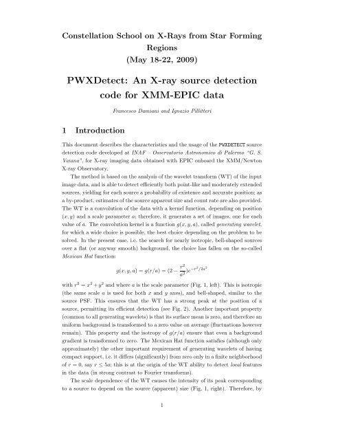
Constellation School on X-Rays from Star FormingRegions(May 18-22, 2009)PWXDetect: An X-ray source detectioncode for XMM-EPIC dataFrancesco Damiani and Ignazio Pillitteri1 IntroductionThis document describes the characteristics and the usage of the PWXDETECT sourcedetection code developed at INAF – Osservatorio Astronomico di Palermo “G. S.Vaiana”, for X-ray imaging data obtained with EPIC onboard the XMM/NewtonX-ray Observatory.The method is based on the analysis of the wavelet transform (WT) of the inputimage data, and is able to detect efficiently both point-like and moderately extendedsources, yielding for each source a probability of existence and accurate position; asa by-product, estimates of the source apparent size and count rate are also provided.The WT is a convolution of the data with a kernel function, depending on position(x, y) and a scale parameter a; therefore, it generates a set of images, one for eachvalue of a. The convolution kernel is a function g(x, y, a), called generating wavelet,for which a wide choice is possible, the best choice depending on the problem to besolved. In the present case, i.e. the search for nearly isotropic, bell-shaped sourcesover a flat (or anyway smooth) background, the choice has fallen on the so-calledMexican Hat function:g(x, y, a) = g(r/a) = (2 − r2a 2 )e−r2 /2a 2with r 2 = x 2 + y 2 and where a is the scale parameter (Fig. 1, left). This is isotropic(the same scale a is used for both x and y axes), and bell-shaped, similar to thesource PSF. This ensures that the WT has a strong peak at the position of asource, permitting its efficient detection (see Fig. 2). Another important property(common to all generating wavelets) is that its surface mean is zero, and therefore anuniform background is transformed to a zero value on average (fluctuations howeverremain). This property and the isotropy of g(r/a) ensure that even a backgroundgradient is transformed to zero. The Mexican Hat function satisfies (although onlyapproximately) the other important requirement of generating wavelets of havingcompact support, i.e. it differs (significantly) from zero only in a finite neighborhoodof r = 0, say r ≤ 5a; this is at the origin of the WT ability to detect local featuresin the data (in strong contrast to Fourier transforms).The scale dependence of the WT causes the intensity of its peak correspondingto a source to depend on the source (apparent) size (Fig. 1, right). Therefore, by1

Figure 4: Examples of exposure map (left panel), and extrapolated border (rightpanel) for the pn detector.3.2 CCD Gaps and EdgesDifferently from ROSAT and Chandra data, the images obtained with the EPICcamera are characterized by sharp gradients in correspondence to the gaps betweenadjacent CCD chips, at the chip outer edges and at bad pixel positions. Thisfeature makes a wavelet detection method prone to find many spurious detectionsin the regions with steep gradients. We have solved the problem with a series of“masks”, computed from the exposure maps. By using these masks, PWXDETECTinterpolates the real image in the gaps and in the bad-pixel holes, using a weightedaverage of values from a small neighborhood with non-zero exposure.Near the image outer edges, the code extrapolates the values of local backgroundoutwards by a 80 ′′ . This extrapolated border avoids obtaining local WT maxima(and thus spurious detections) near the true image edge (Fig. 4).3.3 Combination of different MOS and pn datasetsThe simultaneous availability of three MOS1, MOS2 and pn datasets makes possibleto perform source detection on the combination of the data, to achieve a deepersensitivity than using a single instrument. PWXDETECT can combine severalimages together (not necessarily two MOS and one pn), with weight factors givenby the exposure time (maps) and the detector effective areas (Fig. 5). The WT istherefore applied to an overall count-rate image rather than on photon images. Thedifference is not sensible when dealing with individual detectors, but becomes crucialin the case of a combination of datasets, to compensate for the individual detectorcharacteristics (edge, gaps), and take properly full advantage of the informationcontent of all available data.5

4 Significance threshold of sources and backgroundsimulationsStatistical fluctuations of the background in a real image may give rise local maximain the WT, which might be mistaken as real detections if a detection threshold isnot properly set. A detections threshold is expressed as nσ, where σ is the usualstandard deviation of a Gaussian distribution; actually, since the WT probabilitydistribution is not a Gaussian when the background is Poissonian, a nσ thresholdis meant to be equivalent to a probability level (e.g. 3σ = 99.73%), and we speaktherefore of “equivalent sigmas”. Pre-setting a threshold in terms of some numberof (equivalent) sigmas has only a limited usefulness: a more interesting parameterfor thresholding is the expected number of spurious detections in a given PWXDE-TECT run, which a user is left free to vary according to his/her needs. How thisnumber of spurious detections varies with the nσ threshold needed by PWXDE-TECT has been therefore studied in detail. This was done by running PWXDE-TECT on large sets (several hundreds) of simulated EPIC images containing onlybackground, as already done for the ROSAT/PSPC detection code (Damiani et al.1997), and by studying the distribution of significance for all (spurious) detectedsources. The exposure map was used, by a purposely written simulator, to producemost realistically background vignetting and inter-chip gaps. Both MOS andpn datasets were simulated, and analyzed separately and in combination. We havefound that the threshold corresponding to a given number of spurious detections perfield increases slightly with the background level, parametrized by the total numberof photons in the field of view, and such a dependence was calibrated by analyzingsets of simulations with different total number of counts (for each of MOS and pn).The number of simulated datasets at each background level was large enough to permita reliable derivation of the threshold corresponding to one spurious detectionper field. For a given detector (or combination), the threshold is therefore uniquelyfixed by the desired (average) number of spurious detections per field, and by theimage total background.Indicatively, the threshold corresponding to to one spurious detections per fieldis 4.7-4.8 for images with 100 kcounts, 4.9-5.0 for 150-200 kcounts and 5.2 for 300kcounts, approximately the same for MOS and pn. In case of a sum of datasets, thesame rule applies, provided that the total number of background counts is taken asreference.5 PWXDETECT usagePWXDETECT is able to detect sources on a single EPIC event dataset, or on severalof them with nearly the same pointing. The code needs as input a valid FITSevent file (or a list of event files), and its corresponding exposure map (or list ofexposure maps). The exposure map must be computed beforehand using the SAStask eexpmap, binned (mandatory) at a scale of 2 ′′ pix −1 , resulting in a size of1296×1296 pixels (i.e., a binning of 40 pixels in both X and Y columns of event6

Figure 5: From top to bottom, and from left to right: EPIC MOS1, MOS2, pn, andthe ‘combined’ image obtained with PWXDETECT.tables). Filtering ”on the fly” is not possible: any time or energy filtering must beapplied before calling PWXDETECT.PWXDETECT uses the parameter file pwxdetect.par to read/save its parameters.This file must reside in the working directory and its name cannot be changed.Normally, PWXDETECT asks interactively for input parameters. Non-interactive mode(for e.g. shell scripts) is set by changing in the pwxdetect.par file the mode parameterfrom ’ql’ to ’h’. PWXDETECT requires two important input parameters: the detectionthreshold and the maximum scale to be used in the analysis. The number of expectedspurious detections depends on the choice of these parameters, and on theimage background level (see previous section). The code has been tested mainly onpointlike sources and thus it works with detection scales up to 16 ′′ .5.1 Input parameters and output filesInput file name: a standard EPIC FITS event table, or the name of a file (precededby a ‘@’) containing a list of datasets, one per line.Exposure map file name: the exposure map of the given event file, created witheexpmap, or the name of a file (preceded by a ‘@’) containing a list of exposuremaps, one per line, in exactly the same order as the listed event files.Final significance threshold for detection: the final detection threshold, in equivalentgaussian sigmas (see above). initial threshold: the initial threshold is not askedfor in interactive mode, and its value may be changed only by editing the pwxdetect.parfile. Based on our experience, we recommend that it should be at most oneless than the final threshold (e.g., 3.5 for a final threshold of 4.5), or even slightly7

less.Maximum wavelet scale: the input dataset is convolved with a mexican hat waveletat various spatial scales. The smallest scale is set to 4.0 arcsec to be ≤ the EPICPSF size. The largest scale can be chosen by the user, nominally up to a value of32 ′′ . The scales actually used by PWXDETECT are all powers of √ 2, with other valuesrounded to the nearest power of √ 2. For point sources the value of the maximumuseful wavelet scale is 12-16 ′′ depending on the crowdedness of the field. Maximumscales larger than 16 ′′ are not well tested, and thus not recommended.Output source list filename root: the root file name for detected source lists (andDS9 region file).Output background filename root: the root file name for output background maps.Output Log file name: the file name of a log of PWXDETECT run.The PWXDETECT output comprises the following files:• a list of detected sources (root src, root src.fits), in ASCII and FITS format,respectively, containing source properties (position, counts, count rate, size,exposure time, background value, etc., see below).• an ASCII list which contains for each source and for each scale the detectionsignificance level (root signif)• a DS9-style region file (root overlay.ds9), for visualization of detected sourceswith DS9 (ftools software suite).• a log file containing the same output as printed on the screen.• two FITS background maps: a zero-order map (bkgroot0.fits), and a final map(bkgroot.fits) with bright sources removed. Units are counts/square arcsec.• an image of count rates (rate image.fits) in counts/sec/pixel, and a mask.fitsfile (intermediate products, for checking purposes only).• in case of a sum of images, the following outputs are created: a list of eventswith X and Y coordinates (merged evtlist.fits), and a normalized, summedexposure map (merged expmap.fits),• Optionally, a sensitivity map can be created after the detection process. Thisoption is enabled during code compilation, and thus depends on the codeversion being used. Note: this single step requires normally much more runtime than the usual detection run.Sum of data: Inputs and outputs:In the case of a sum, a list of datasets is processed. The detector of the first datasetis used as reference instrument and the other datasets are scaled (through factorsinput by the user) to this reference detector.The input file names must be preceded by a “@” symbol (e.g.:“@maplist” toread in the maplist file); in this way the code reads the list files of event tables8

and maps. To combine several dataset (for example MOS1, 2 and pn) the exposuremap list file must contain two numbers after each exposure map file name(in the same line): a number proportional to the respective background levels inthe input datasets, important to ensure that no unexpected spurious detectionsare obtained in combining them; and an effective area (in cm 2 ) for each detector(either monochromatic or spectrum-weighted, as chosen by the user), used to scalethe count rates to the reference detector, to derive the X-ray photon flux for detectedsources. The first number can be the total number of events in each dataset(assuming that background counts are much more than total source counts, otherwiseit should be evaluated more accurately). The second number should be themean effective area of each detector, weighted with the spectrum of sources thatare expected to be found (or those that one aims to study with more accuracy).Exposure times listed in the output files are the simple sum of exposure timesof each map, while the rates and counts are calculated by taking into account theweighted sum of the different detector responses and vignetting. They are scaledto the reference detector, hence to derive the energy fluxes (ergs cm −2 s −1 ) theconversion factor between count rates and energy fluxes must be calculated for thatreference detector and for the corresponding filter used during that observation.Obviously, changing the order of the listed datasets changes the reference detector.The nominal pointing direction of the combined image merged evtlist.fits is thesame as the input image with the highest count statistics.5.2 The output file root srcThe detected source file root src[.fits] contains:Column # 1: RA (deg): Right Ascension (decimal degrees)Column # 2: RA_err (deg): Error on RA (decimal degrees)Column # 3: Dec (deg): Declination (decimal degrees)Column # 4: Dec_err (deg): Error on Dec (decimal degrees)Column # 5: X (pix): Position X (physical pixels)Column # 6: X_err (pix): Error on X (physical pixels)Column # 7: Y (pix): Position Y (physical pixels)Column # 8: Y_err (pix): Error on Y (physical pixels)Column # 9: Offax (arcmin): Off-axis angleColumn #10: Det_scale (arcsec): Highest-significance detection scaleColumn #11: Src_area (arcsec 2 ): Approximate source (core) areaColumn #12: Signif: Detection significance (sigmas)Column #13: Src_cnt: Total source countsColumn #14: Cnt_err: Error on source countsColumn #15: Bkg_cnt: Background counts in source core areaColumn #16: Src_ct_rate (cts/sec): Source count rateColumn #17: Src_rate_err (cts/sec): Error on source count rateColumn #18: Src_flux (cts/sec/cm 2 ): Source photon fluxColumn #19: Src_flux_err (cts/sec/cm 2 ): Error on source fluxColumn #20: Bkg_rate (cts/sec/arcsec 2 ): Background count rate9

Column #21: Exp_time (sec): Source size-weighted exposure timeColumn #22: Size (arcsec): Source sizeColumn #23: Siz_err (arcsec): Error on source sizeColumn #24: Extent: Source extent (relative to PSF)Column #25: Ext_err: Error on source extentColumn #26: Src_num: PWXDETECT source number6 Preparation of dataThis section describes how to filter the data in order to maximize the ability to detectfaint sources by reducing the background level and spurious artifacts in EPICimages. The data can be obtained by the Pipeline Processed System (PPS files) orby having to rerun the reduction chains for MOS and pn starting from ObservationData Files (ODF files). Details on the general processing of EPIC data can be foundin the document at the web address: http://heasarc.gsfc.nasa.gov/docs/xmm/abc/.We suppose to start from event tables generated by the SAS pipeline reduction softwareor retrieved from PPS files. We give here further details about energy, patternand time filtering.Generally, the data from the standard SAS pipeline reduction need to be filteredfor energy band, pixel triggering pattern and time intervals with low backgroundrate. The SAS task evselect is used throughout these steps. An example of emevselect command is the following:evselect \--table=’P0041750101PNS002PIEVLI0000.FIT’ \--withfilteredset=true \--filteredset=filteredPN_03.79.fits \--keepfilteroutput=true \--destruct=yes \--withimageset=false \--writedss=true \expression="!( (CCDNR.eq.5) .and. (RAWX.eq.11)) .and. ((FLAG & 0xfb0024)==0) \.and. (PATTERN .LE. 12) .and. (PI.ge.300) .and. (PI.le.7900)This command will filter the event table P0041750101PNS002PIEVLI0000.FITto obtain the filtered file filteredPN 03.79.fits with the criteria given in the expressionparameter. The expression operates a selection on FLAG and PATTERNparameters, energy band and excludes a group of pixels.The filters which should be applied to the initial data are described below.Pattern selection. A “pattern” flag is assigned to each event in order to qualifythe manner in which neighbour detector pixels have been triggered simultaneouslyby each X-ray photon. A convenient choice is to retain only the events that triggeredup to four pixels at the same time (in fortran-like syntax: PATTERN .le. 12). Forspectral analysis a restrictive choice is PATTERN .le. 4 to retain only double pixelevents.10

Energy filter. This filter selects the events in a certain energy band throughthe PI column (PI units are eV).FLAG filter. In Fig. 6, left panel, the raw image is affected by spuriouspseudo-events near the chip edges and by hot pixels. Such features could resultin many spurious detected sources. It is of particular relevance to clean the imagefrom these effects if we are interested to obtain a list of detected sources almost freefrom false detections. It is possible to filter the event by means of FLAG column inMOS and pn. The expression to be used is written in the keyword XMMEA EM andXMMEA EP in the header of event FITS table for MOS and pn respectively. Whilefor MOS data the filtering with this expression (namely: FLAG & 0x766b0000)==0)is adeguate, for pn data the analog expression: FLAG & 0xfa0000) == 0 is not.The various flag listed in the header keywords correspond to expressions given inexadecimal notation. The (exadecimal) sum of two values performs the combinedaction of the summed flag filters. The expression FLAG & 0xfb0024)==0) makesthe above pn selection and in addiction excludes the events: out of fov, close tochip gaps, close to bad pixels; namely, the sum of exadecimal values: (0x)fa0000 +(0x)4 + (0x)20 + (0x)010000. The right panel in Fig. 6 shows the result of thesefilters.Bad pixels. It is possible to exclude group of pixels or entire chip columns. Inthe above example the section !((CCDNR.eq.5) .and. (RAWX.eq.11)) exclude thedamaged column 11 of chip 5. This bad column is the bright one in the top leftcorner of raw image in Fig. 6, left panel.6.1 Time filteringXMM-Newton observations are very often affected by high background rate intervals.Because of the high satellite effective area, during high solar activity episodes,high energy particles are collected by the XMM-Newton mirrors and produce contaminantevents. We discuss in more detail this filtering stage and a method basedon the signal to noise of the image.7 ReferencesThe algorithm and the application to the PSPC detector are described in:– Damiani et al. 1997, ApJ, 483, 350– Damiani et al. 1997, ApJ, 483, 370For technical and calibration information about EPIC and XMM-Newton:http://xmm.vilspa.esa.es11

Figure 6: Left panel: pn data from SAS reduction pipeline. Right panel: the samedata filtered for energy, flag, pattern and low background rate intervals.12