keck geology consortium proceedings of the twenty-fourth annual ...

KECK GEOLOGY CONSORTIUM 

PROCEEDINGS OF THE TWENTY-FOURTH 

ANNUAL KECK RESEARCH SYMPOSIUM IN 

GEOLOGY 

April 2011 

Union College, Schenectady, NY 

Dr. Robert J. Varga, Editor 

Director, Keck Geology Consortium 

Pomona College 

Dr. Holli Frey 

Symposium Convenor 

Union College 

Carol Morgan 

Keck Geology Consortium Administrative Assistant 

Diane Kadyk 

Symposium Proceedings Layout & Design 

Department of Earth & Environment 

Franklin & Marshall College 

Keck Geology Consortium 

Geology Department, Pomona College 

185 E. 6 th St., Claremont, CA 91711 

(909) 607-0651, keckgeology@pomona.edu, keckgeology.org 

ISSN# 1528-7491 

The Consortium Colleges The National Science Foundation ExxonMobil Corporation

KECK GEOLOGY CONSORTIUM 

PROCEEDINGS OF THE TWENTY-FOURTH ANNUAL KECK 

RESEARCH SYMPOSIUM IN GEOLOGY 

ISSN# 1528-7491 

Robert J. Varga 

Editor and Keck Director 


April 2011 



185 E 6 th St., Claremont, CA 

91711 

Diane Kadyk 

Proceedings Layout & Design 

Franklin & Marshall College 

Keck Geology Consortium Member Institutions: 

Amherst College, Beloit College, Carleton College, Colgate University, The College of Wooster, 

The Colorado College, Franklin & Marshall College, Macalester College, Mt Holyoke College, 

Oberlin College, Pomona College, Smith College, Trinity University, Union College, 

Washington & Lee University, Wesleyan University, Whitman College, Williams College 

2010-2011 PROJECTS 

FORMATION OF BASEMENT-INVOLVED FORELAND ARCHES: INTEGRATED STRUCTURAL AND 

SEISMOLOGICAL RESEARCH IN THE BIGHORN MOUNTAINS, WYOMING 

Faculty: CHRISTINE SIDDOWAY, MEGAN ANDERSON, Colorado College, ERIC ERSLEV, University of 

Wyoming 

Students: MOLLY CHAMBERLIN, Texas A&M University, ELIZABETH DALLEY, Oberlin College, JOHN 

SPENCE HORNBUCKLE III, Washington and Lee University, BRYAN MCATEE, Lafayette College, DAVID 

OAKLEY, Williams College, DREW C. THAYER, Colorado College, CHAD TREXLER, Whitman College, TRIANA 

N. UFRET, University of Puerto Rico, BRENNAN YOUNG, Utah State University. 

EXPLORING THE PROTEROZOIC BIG SKY OROGENY IN SOUTHWEST MONTANA 

Faculty: TEKLA A. HARMS, JOHN T. CHENEY, Amherst College, JOHN BRADY, Smith College 

Students: JESSE DAVENPORT, College of Wooster, KRISTINA DOYLE, Amherst College, B. PARKER HAYNES, 

University of North Carolina - Chapel Hill, DANIELLE LERNER, Mount Holyoke College, CALEB O. LUCY, 

Williams College, ALIANORA WALKER, Smith College. 

INTERDISCIPLINARY STUDIES IN THE CRITICAL ZONE, BOULDER CREEK CATCHMENT, 

FRONT RANGE, COLORADO 

Faculty: DAVID P. DETHIER, Williams College, WILL OUIMET. University of Connecticut 

Students: ERIN CAMP, Amherst College, EVAN N. DETHIER, Williams College, HAYLEY CORSON-RIKERT, 

Wesleyan University, KEITH M. KANTACK, Williams College, ELLEN M. MALEY, Smith College, JAMES A. 

MCCARTHY, Williams College, COREY SHIRCLIFF, Beloit College, KATHLEEN WARRELL, Georgia Tech 

University, CIANNA E. WYSHNYSZKY, Amherst College. 

SEDIMENT DYNAMICS & ENVIRONMENTS IN THE LOWER CONNECTICUT RIVER 

Faculty: SUZANNE O’CONNELL, Wesleyan University 

Students: LYNN M. GEIGER, Wellesley College, KARA JACOBACCI, University of Massachusetts (Amherst), 

GABRIEL ROMERO, Pomona College. 

GEOMORPHIC AND PALEOENVIRONMENTAL CHANGE IN GLACIER NATIONAL PARK, 

MONTANA, U.S.A. 

Faculty: KELLY MACGREGOR, Macalester College, CATHERINE RIIHIMAKI, Drew University, AMY MYRBO, 

LacCore Lab, University of Minnesota, KRISTINA BRADY, LacCore Lab, University of Minnesota

Students: HANNAH BOURNE, Wesleyan University, JONATHAN GRIFFITH, Union College, JACQUELINE 

KUTVIRT, Macalester College, EMMA LOCATELLI, Macalester College, SARAH MATTESON, Bryn Mawr 

College, PERRY ODDO, Franklin and Marshall College, CLARK BRUNSON SIMCOE, Washington and Lee 

University. 

GEOLOGIC, GEOMORPHIC, AND ENVIRONMENTAL CHANGE AT THE NORTHERN 

TERMINATION OF THE LAKE HÖVSGÖL RIFT, MONGOLIA 

Faculty: KARL W. WEGMANN, North Carolina State University, TSALMAN AMGAA, Mongolian University of 

Science and Technology, KURT L. FRANKEL, Georgia Institute of Technology, ANDREW P. deWET, Franklin & 

Marshall College, AMGALAN BAYASAGALN, Mongolian University of Science and Technology. 

Students: BRIANA BERKOWITZ, Beloit College, DAENA CHARLES, Union College, MELLISSA CROSS, Colgate 

University, JOHN MICHAELS, North Carolina State University, ERDENEBAYAR TSAGAANNARAN, Mongolian 

University of Science and Technology, BATTOGTOH DAMDINSUREN, Mongolian University of Science and 

Technology, DANIEL ROTHBERG, Colorado College, ESUGEI GANBOLD, ARANZAL ERDENE, Mongolian 

University of Science and Technology, AFSHAN SHAIKH, Georgia Institute of Technology, KRISTIN TADDEI, 

Franklin and Marshall College, GABRIELLE VANCE, Whitman College, ANDREW ZUZA, Cornell University. 

LATE PLEISTOCENE EDIFICE FAILURE AND SECTOR COLLAPSE OF VOLCÁN BARÚ, PANAMA 

Faculty: THOMAS GARDNER, Trinity University, KRISTIN MORELL, Penn State University 

Students: SHANNON BRADY, Union College. LOGAN SCHUMACHER, Pomona College, HANNAH ZELLNER, 

Trinity University. 

KECK SIERRA: MAGMA-WALLROCK INTERACTIONS IN THE SEQUOIA REGION 

Faculty: JADE STAR LACKEY, Pomona College, STACI L. LOEWY, California State University-Bakersfield 

Students: MARY BADAME, Oberlin College, MEGAN D’ERRICO, Trinity University, STANLEY HENSLEY, 

California State University, Bakersfield, JULIA HOLLAND, Trinity University, JESSLYN STARNES, Denison 

University, JULIANNE M. WALLAN, Colgate University. 

EOCENE TECTONIC EVOLUTION OF THE TETONS-ABSAROKA RANGES, WYOMING 

Faculty: JOHN CRADDOCK, Macalester College, DAVE MALONE, Illinois State University 

Students: JESSE GEARY, Macalester College, KATHERINE KRAVITZ, Smith College, RAY MCGAUGHEY, 

Carleton College. 

Funding Provided by: 

Keck Geology Consortium Member Institutions 

The National Science Foundation Grant NSF-REU 1005122 

ExxonMobil Corporation

Keck Geology Consortium: Projects 2010-2011 

Short Contributions— Front Range, CO 

INTERDISCIPLINARY STUDIES IN THE CRITICAL ZONE, BOULDER CREEK CATCHMENT, 

FRONT RANGE, COLORADO 

Project Faculty: DAVID P. DETHIER: Williams College, WILL OUIMET: University of Connecticut 

CORING A 12KYR SPHAGNUM PEAT BOG: A SEARCH FOR MERCURY AND ITS IMPLICATIONS 

ERIN CAMP, Amherst College 

Research Advisor: Anna Martini 

EXAMINING KNICKPOINTS IN THE BOULDER CREEK CATCHMENT, COLORADO 

EVAN N. DETHIER, Williams College 

Research Advisor: David P. Dethier 

THE DISTRIBUTION OF PHOSPHORUS IN ALPINE AND UPLAND SOILS OF THE BOULDER 

CREEK, COLORADO CATCHMENT 

HAYLEY CORSON-RIKERT, Wesleyan University 

Research Advisor: Timothy Ku 

RECONSTRUCTING THE PINEDALE GLACIATION, GREEN LAKES VALLEY, COLORADO 

KEITH M. KANTACK, Williams College 


CHARACTERIZATION OF TRACE METAL CONCENTRATIONS AND MINING LEGACY IN SOILS, 

BOULDER COUNTY, COLORADO 

ELLEN M. MALEY, Smith College 

Research Advisor: Amy L. Rhodes 

ASSESSING EOLIAN CONTRIBUTIONS TO SOILS IN THE BOULDER CREEK CATCHMENT, 

COLORADO 

JAMES A. MCCARTHY, Williams College 


USING POLLEN TO UNDERSTAND QUATERNARY PALEOENVIRONMENTS IN BETASSO GULCH, 

COLORADO 

COREY SHIRCLIFF, Beloit College 

Research Advisor: Carl Mendelson 

STREAM TERRACES IN THE CRITICAL ZONE – LOWER GORDON GULCH, COLORADO 

KATHLEEN WARRELL, Georgia Tech 

Research Advisor: Kurt Frankel 

METEORIC 10 BE IN GORDON GULCH SOILS: IMPLICATIONS FOR HILLSLOPE PROCESSES AND 

DEVELOPMENT 

CIANNA E. WYSHNYSZKY, Amherst College 

Research Advisor: Will Ouimet and Peter Crowley 



185 E. 6 th St., Claremont, CA 91711 

Keckgeology.org

24th Annual Keck Symposium: 2011 Union College, Schenectady, NY 

INTERDISCIPLINARY STUDIES IN THE CRITICAL ZONE, 

BOULDER CREEK CATCHMENT, FRONT RANGE, COLORADO 

DAVID P. DETHIER, Williams College 

WILL OUIMET, University of Connecticut 

INTRODUCTION 

Processes in the critical zone, the life-sustaining surficial 

mantle of the earth, involve weathered geologic 

materials, water, and the biosphere, mediated by 

atmospheric processes that are controlled by changing 

climate. Field and laboratory studies that investigate 

geologic, hydrologic and geochemical components of 

the critical zone provide valuable data about processes 

and the physical basis for their integration into 

models of short and long-term geomorphic, hydrologic 

and biochemical response. The Keck Colorado 

Project is working in cooperation with a large 

interdisciplinary study of the critical zone (Boulder 

Creek Critical Zone Observatory: Weathered profile 

development in a rocky environment and its influence 

on watershed hydrology and biogeochemistry— Suzanne 

Anderson, PI, Institute for Arctic and Alpine 

Studies, University of Colorado). The observatory 

(CZO) consists of 3 small, instrumented catchments 

in the Boulder Creek basin, Colorado Front Range: 

(1) Green Lakes Valley (GLV; el. 3400 m)--a steep, 

glacially scoured alpine area in the City of Boulder 

watershed; (2) Gordon Gulch (el. 2600 m)--a forested, 

mid-elevation catchment that exposes isolated bedrock 

remnants (tors) developed on a surface of low 

relief; and (3) Betasso gulch (el. 1950 m)--a steep, 

thinly forested basin that preserves thick regolith in 

the upper catchment and exposes extensive bedrock 

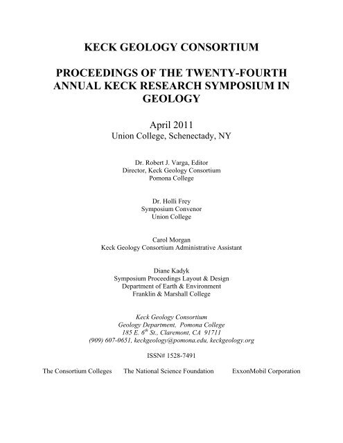
outcrops at lower elevations (Fig. 1). 

The glaciated GLV, low relief surface, and bedrock 

canyons are developed in granitic or gneissic rocks 

and are influenced by the strong gradient in elevation, 

climate and vegetation from west to east. Variation 

in critical-zone development in these different environments 

allows us to test models of weathering and 

regolith generation, elemental cycling, slope evolution 

and sediment transport in an accessible field 

setting. Land-use, vegetation and hydrologic response 

93 

in each CZO catchment also reflect changes produced 

by anthropogenic activities such as mining and timber 

harvest over the past 150 years. Keck Colorado field 

studies focus on using a variety of techniques to map 

and characterize the geologic history, near-surface 

geologic materials and geochemical properties for 

each of the study catchments. 

Figure 1. Perspective view looking west across the Front 

Range from Boulder, Colorado, showing Middle Boulder 

Creek and location of Betasso, Gordon Gulch and Green 

Lakes Valley catchments, Boulder Creek Critical Zone 

Observatory. White filled area shows approximate extent 

of latest Pleistocene glaciers (after Madole et al., 1999). 

SETTING 

The middle Boulder Creek catchment (Fig. 1) extends 

from the glaciated alpine zone of the Continental 

Divide east to the semi-arid western edge of the Great 

Plains. The high-relief zone of cirques and deep, Ushaped 

valleys in the glaciated area become shallower 

eastward through a zone of low relief and relatively 

low slopes. To the east, valleys deepen into steep, 

narrow bedrock canyons as they pass knickzones, and 

flatten to lower channel slopes near the piedmont margin. 

Small glaciers and late-persisting snowfields dot 

the alpine zone, which exposes bedrock and relatively 

thin deposits related to the latest Pleistocene Pinedale 

glaciation and to Holocene erosion. The forested zone


of low relief exposes local areas of thick (characteristically 

3 to 8 m) regolith, saprolite and oxidized bedrock, 

but the weathered mantle is thin in other areas. 

Low terraces and alluvial fans as thick as 4 m line 

channels locally. In the vicinity of knickzones and 

in downstream areas such as Betasso gulch, slopes 

near channels are steep and fresh bedrock is exposed, 

whereas areas more distant from channels retain a 

thicker weathered mantle. 

APPROACH 

In our third project year, we used field mapping and 

sampling in all three CZO catchments, supplemented 

by geophysical measurements, in order to provide 

basic data about soils and their geochemistry, shallow 

subsurface geology and erosional history of 

the critical zone. Students supported by the Keck 

Geology consortium and by NSF learned geophysical 

techniques and initial data reduction, processing 

and visualization methods in these settings. Students 

chose from a variety of potential projects in the study 

catchments; 2010 project topical areas included: 

1. Trace-metal studies of soils and bog sediment, 

Boulder Creek catchment 

2. Soil chemistry (Fe and P) in CZO catchments 

and meteoric 10Be studies of soils, focused on 

Gordon Gulch 

3. Stratigraphy and palynology of valley-fill 

sediment, Gordon and Betasso catchments 

4. Geomorphic research: Ice erosion and geo 

morphic evolution of the Green Lakes Valley 

and the evolution of knickpoints along channels 

in the Boulder Creek catchment 

We ran resistivity lines in Gordon Gulch, resistivity 

and ground-penetrating radar on Niwot Ridge and 

ground-penetrating radar in the vicinity of the bogs 

near the N. Branch Boulder Creek. In Gordon Gulch, 

we worked on regolith studies in cooperation with 

investigators from the University of Colorado and the 

US Geological Survey. 

STUDENT PROJECTS 

Six Keck students joined Williams students Evan 

Dethier, Keith Kantack and James McCarthy and 

94 

Erin Camp (Amherst), who were supported directly 

by NSF funding. David Dethier and Will Ouimet 

supervised students on a daily basis and field teams 

frequently joined investigators and graduate students 

from the University of Colorado. Matthias Leopold 

(Technical University of Munich) worked with Keck 

students for two weeks in the field. Keck students 

were among the only undergraduates to present preliminary 

results of their field research at the 3rd annual 

Boulder Creek CZO meeting on 10 August 2010. 

Keck Colorado students worked in pairs on a daily 

basis and sometimes as geophysical support teams. 

Geophysical data provided important background data 

for extensive studies in Gordon Gulch and for coring 

of bogs (Fig. 2). 

Figure 2. Coring a bog in a late Pinedale moraine complex 

along the N. Fork Boulder Creek, supervised by 

Robert Nelson, Colby College. 

Short papers elsewhere in this volume report results 

of the field and laboratory studies in some detail. 

We summarize and provide brief comments on this 

research here. 

Studies of trace metals in organic sediment, soil 

and regolith in Gordon Gulch and adjacent areas 

Erin Camp (Amherst) reports “Coring a 12 kyr sphagnum 

bog in the N. Boulder Creek valley—a search 

for mercury and its implications” and Ellie Maley 

(Smith) worked on “Characterization of trace metal 

concentrations and mining legacy in soils, Boulder 

County, Colorado”. Both of these studies demonstrate 

that Hg is enriched in recent organic-rich


sediment of the montane zone when compared to 

older bog sediment or to soil C-horizons. The bog Hg 

profile and 14 C ages show a strong correspondence 

between elevated Hg levels and large, silicic volcanic 

eruptions in Holocene time. Peak Hg levels produced 

by eruptions decline over narrow intervals. Mercury 

concentrations in bog sediments increase to a broad 

peak coincident with exploitation of precious metals 

in the western hemisphere beginning in the 16th century 

and peaking in the late 19th century in Colorado. 

Ellie’s work shows that Hg, As and possibly Pb are 

enriched in organic-rich O and A-horizons compared 

to soil parent material; other minor elements such as 

Cu and Zn do not show enrichment. Ellie’s research 

suggests that metal enrichment likely represents the 

legacy of local metal mining, milling and smelting, 

and the affinity of organic matter for these relatively 

volatile trace metals. 

Studies of soil and regolith geochemistry and age 

in Gordon Gulch and adjacent areas 

Four students, including Ellie Maley, studied soils 

and regolith exposed in pits that were dug in Gordon 

Gulch and at other nearby exposures. The “pit 

crew”, aided by their advisors and other CZO investigators, 

collected from many of the same sites and 

worked on separate, but complimentary topics. Cianna 

Wyshnytzky (Amherst) documented meteoric 

10 Be accumulation in soils from Gordon Gulch and 

at Silver Lake—“Erosion, particle paths and deposition—meteoric 

10 Be in Gordon Gulch”. James 

McCarthy (Williams) studied the texture and Fed 

(dithionite-extractable iron) accumulation in soils 

from Gordon Gulch and adjacent subalpine and alpine 

areas: “Assessing eolian contributions to soils in the 

Boulder Creek catchment”, whereas Hayley Corson- 

Rikert (Wesleyan) studied “Extractable P in soils of 

the Boulder Creek catchment, Colorado”. 

Data from these studies demonstrate that there are 

fundamental differences between soils developed on 

stable sites and those that formed on regolith-covered 

hillslopes and that dustfall and chemical weathering 

influence the partitioning of Fed and P in soils. Both 

erosion and weathering rates are related to aspect in 

Gordon Gulch; regolith is thicker, more weathered 

and contains more meteoric 10 Be on the north-facing 

95 

Figure 3. Soil pits in Gordon Gulch. A. James McCarthy, 

Cianna Wyshnytzky, Hayley Corson-Rikert and Ellie 

Maley in a 1.8 m-deep pit in regolith, north-facing slope. 

B. Soil-sampling tools and thin regolith over saprolite, 

south-facing slope. Cianna Wyshnytzky sampling for meteoric 

10Be analysis. 

slope. Fe and P mobility also are influenced by the 

moisture and temperature gradient between soils exposed 

in Gordon Gulch and soils of similar age in the 

alpine and subalpine portions of the Boulder Creek 

CZO. Extractable Fe, clay and 10 Be reach peak values 

in the B-horizon of the till-derived soil at Silver Lake 

(Fig. 4), whereas P is depleted in the soil compared to 

unweathered till; soils in Gordon Gulch and Betasso 

do not display comparable patterns. 

The inventory of meteoric 10 Be in Gordon Gulch is 

consistent with model predictions for deposition rates 

(Graly et al., 2011), but the inventory at Silver Lake is 

too high, suggesting that at this site dustfall rates or


Figure 4. Plot showing relationship of Fed, clay and 

meteoric 10 Be to depth below the surface and soil horizons 

at Silver Lake, Green Lakes Valley. P (not plotted) is depleted 

and relatively labile in the upper soil and relatively 

enriched and associated with inorganic material in the 

unoxidized till. 

late Pleistocene precipitation may have been substantially 

higher than at present. Cianna’s meteoric 10 Be 

research represents the first application of this technique 

in the Boulder Creek CZO catchments. 

Stratigraphy and palynology of valley-fill sediment, 

Gordon and Betasso catchments 

In Gordon Gulch and in upper Betasso Gulch, colluvium 

and deposits beneath terraces as much as 4 

m above the channel comprise local valley fills of 

Holocene and latest Pleistocene (?) age. Kathleen 

Warrell (Georgia Tech) studied terrace morphology 

and sampled deposits exposed beneath low terraces 

in Gordon Gulch-- “Stream terraces in the critical 

zone-- lower Gordon Gulch, Colorado”. Her work 

96 

shows that at least 75,000 m 3 of sediment is stored in 

near the channel in lower Gordon Gulch. Sediment 

beneath the 1-m terrace is less than 1500 years old 

(Fig. 5); 

Figure 5. Graphic log of sediment (description from C. 

Shircliff) exposed beneath K. Warrell’s 1-m terrace. Basal 

sediment is approximately 1500 years old. 

higher terraces are cut into middle and early Holocene 

alluvial and colluvial deposits. Corey Shircliff 

(Beloit) studied organic material in Holocene terrace 

deposits in Gordon Gulch and Betasso--“Using pollen 

to understand Quaternary paleoenvironments in 

Betasso Gulch, Colorado”. She was able to separate 

pollen from a buried soil developed on colluvium and 

to identify many of the pollen grains. Corey’s work 

indicates that early Holocene pollen at Betasso is 

richer in Picea (spruce) than a modern pollen sample 

and records a climate that was likely wetter and perhaps 

slightly cooler than that at present. 

Ice erosion and geomorphic evolution of the Green 

Lakes Valley and the evolution of knickpoints 

along channels in the Boulder Creek catchment 

Keith Kantack (Williams) used field measurements


in GLV and interpretation of DEMs derived from 

Lidar flown in August 2011 to map the extent of late 

Pinedale ice and glacial moraines in the upper North 

Boulder Creek catchment (Fig. 6). 

Figure 6. Keith Kantack, Evan Dethier and James Mc- 

Carthy stand on glacially sculpted and smoothed bedrock 

knob, upper Green Lakes Valley. 

His work “Reconstructingthe Pinedale glaciation in 

the Green Lakes valley, Colorado” shows that latest 

Pleistocene ice in the GLV was thin (mainly less 

than 150 m), but extended out of the cirques and 

more than 10 km to the east to elevations as low as 

2650 m. Measured moraine volumes suggest that the 

average erosion rate by North Boulder cirque glaciers 

was about 1mm yr -1 during the maximum late Pinedale 

glaciation, which lasted from about 21 to 15 ka. 

Those rates are similar to estimates used by Ward et 

al. (2009) for modeling ice flow in Front Range catchments. 

Evan Dethier studied the evolution of channels and 

slopes at different scales near knickpoints in Betasso, 

Gordon Gulch, and along Middle Boulder Creek-- 

“Knickpoints—a study of channels in the Boulder 

Creek catchment”. His field studies, combined with 

RiverTools interpretation of DEMs derived from August, 

2010 Lidar, suggest that channels and adjacent 

hillslopes reflect the slow migration of knickpoints 

in the Boulder Creek catchment, moderated by local 

rock strength. Betasso gulch, the smallest of the 

Boulder Creek CZO catchments, has a channel that is 

97 

steep and rough throughout and is flanked by steep, 

smooth slopes that expose bedrock and thin regolith 

near Boulder Creek. In the upper part of the catchment, 

however, the channel only locally exposes 

bedrock, and is cut mainly in soft, deeply weathered 

saprolite and through thick colluvium that was deposited 

in latest Pleistocene time. At Gordon Gulch, rock 

strength appears to control the location of the knickzone 

that separates the upper and lower basin; morphology 

of adjacent hillslopes reflect local channel 

slope. At the scale of Boulder Creek, hillslope evolution 

appears to “lag” knickpoint migration because 

local rocks are strong and hillslope erosion requires 

removal of large volumes of rock. 

Figure 7. Sculpted bedrock and boulder-rich channel 

in the knickzone along N. Boulder Creek above Boulder 

Falls. 

CONCLUSIONS 

“Piggybacking” the Keck Colorado Geology Project 

on the NSF-Boulder Creek Critical Zone Observatory 

has allowed Keck undergraduates to integrate their 

projects with the research of graduate and postdoctoral 

students from the University of Colorado and 

other research universities. Keck student research 

has benefitted from the personnel, monitoring efforts, 

and general level of scientific interest associated with 

the NSF project. The Boulder Creek CZO has gained 

from the focused field and laboratory research of the 

Keck students, their energy, and their collective demonstration 

of what can be accomplished by the best


undergraduates. 

ACKNOWLEDGMENTS 

Field studies and measurements in the Boulder Creek 

area were performed in cooperation with the Boulder 

Creek CZO Project (National Science Foundation), 

the USDA Forest Service, and the City of Boulder 

Watershed and Parks and Recreation Departments. 

Nel Caine (University of Colorado) and Craig Skeie 

(City Watershed Manager) guided work in the Green 

Lakes basin, Pete Birkeland (University of Colorado) 

taught us about soils. Greg Tucker, Cam Wobus and 

Abby Langston (all affiliated with the University of 

Colorado) shared their knowledge of the Critical Zone 

and how to study it. Suzanne Anderson and Bob Anderson 

joined us for many field “teaching moments”. 

We gratefully acknowledge the field and laboratory 

skills of Bob Nelson (Colby College), and the ongoing 

cooperation, digging ability and cogent advice of 

Joerg Voelkel and Matthias Leopold (Technical University 

of Munich). The hospitality of the Mountain 

Research Station made this project possible. 

REFERENCES 

Graly, J. A., Reusser, L. J., and Bierman, P. R., 2011, 

Short and long-term delivery rates of meteoric 

10Be to terrestrial soils: Earth and Planetary 

Science Letters 302, p. 329-336. 

Madole, R.F., VanSistine, D.P., and Michael, J. A., 

1999, Pleistocene glaciation in the upper Platte 

River drainage basin, Colorado. U.S. Geol. Surv. 

Geol. Invest. Series I-2644. 

Ward, D. J., R. S. Anderson, Z. S. Guido, and J. P. 

Briner (2009), Numerical modeling of cosmogenic 

deglaciation records, Front Range and San 

Juan mountains, Colorado, J. Geophys. Res., 

114, F01026, doi:10.1029/2008JF001057. 

98


CORING A 12KYR OMBROTROPHIC SPHAGNUM PEAT BOG: 

A HISTORY OF ATMOSPHERIC MERCURY 

ERIN CAMP, Amherst College 

Research Advisor: Anna Martini 

INTRODUCTION 

Elemental mercury (Hg 0 ) is primarily transported 

through the atmosphere, where it has an average 

residence time of one year and can be deposited 

worldwide (Bindler, 2003). Hg 0 is deposited both 

naturally and anthropogenically in the environment, 

where it can chemically transform into a highly toxic 

methylated form of mercury (Vandal et al., 1993). 

Mercury is introduced naturally into the environment 

through volcanism, geothermal activity, and emission 

from the biosphere and water bodies, and anthropogenically 

through coal combustion, waste incineration, 

and metal ore processing (Bindler, 2003). Additionally, 

mercury retention is known to increase in 

colder temperatures, thus can be used as a paleotemperature 

proxy (Martínez-Cortizas et al., 1999). 

Ombrotrophic peat bogs topped by Sphagnum moss 

are excellent archives of elemental Hg deposition 

because they receive all their nutrients from the 

atmosphere and allow little vertical mixing (Madsen, 

1981; Lodenius et al., 1983). The Colorado Front 

Range has a rich history of gold and silver mining, 

smelting and mercury amalgamation, thus it is an 

ideal location for mercury studies (Nriagu, 1994). 

This project has measured the amount of Hg deposition 

in North Boulder Creek Bog, CO in order to 1) 

identify the natural background Hg deposition for 

this location, 2) correlate concentrations with natural 

and anthropogenic historical events, and 3) calculate 

the amount of anthropogenically deposited mercury 

in this location. 

PROJECT LOCATION 

North Boulder Creek Bog (40.007349º,-105.560421º; 

Fig. 1) is a 3-meter deep subalpine Sphagnum mosscoated 

ombrotrophic bog that began to accumulate 

organic sediment at 12,000 cal. 14 C years BP (yBP; 

99 

Figure 1: Google Earth image of project location, 

illustrating the perimeter of the bog and the surrounding 

glacial moraine. 

present refers to 1950) (Leopold and Dethier, 2007; 

Leopold, 2010 personal communication). The bog 

is located in the Front Range of Colorado, situated 

within a kettle hole associated with the Pinedale 

glaciation, and flanked by a glacial moraine on its 

eastern side (Richmond, 1960; Fig. 1). North Boulder 

Creek Bog is believed to have formed after the 

rapid drainage of Lake Devlin about 13,000 years 

ago (Leopold pers. comm. 2010; Madole, 1985). 

METHODS 

The coring, performed with a modified Livingstone 

piston corer (Livingstone, 1955), produced a complete 

1.8m core that had been compacted by an average 

of 50%—slightly less near the top and more 

near the bottom—representing a 3.65m core. Sampling 

of the core was performed at 2.5cm intervals, 

representing ‘expanded’ intervals of 5cm. All depths 

referred to in this paper are ‘expanded’ depths. All 

samples were dried overnight—maximum of 12 

hours—at 105ºC. All seventy-four samples were


ground with mortar and pestle, and run individually 

in a direct combustion cold vapor AA instrument 

(Hydra-C, Leeman Labs) for total mercury concentration. 

The machine was calibrated using a marine 

sediment standard with a precision of ±6.03% and an 

accuracy (recovery) of 103.6%. Following these runs, 

higher resolution sampling was conducted at 2cm 

‘expanded’ intervals near the uppermost section of the 

core, in order to obtain more precise data during 

modern times. Six samples were taken near 35cm 

depth, and five additional samples were taken from 

the top 5cm of the core. Additionally, five samples 

were sent to the Woods Hole NOSAMS Facility for 

AMS radiocarbon analysis. These samples were extracted 

from various locations along the core at 100, 

160, 265, 315, and 365cm depths. Radiocarbon age is 

calculated from the δ13C-corrected Fraction Modern 

(Fm) according to the following formula: 

Age = -8033ln (Fm). 

Figure 2: Photos of top two sections of the core. Top 

photo represents the first meter of core, compacted to 

48cm. Bottom picture represents the second meter of core, 

compacted to 46cm. 

RESULTS 

The radiocarbon data yield a typical, slightly curved 

age vs. depth trend. With a linear regression analysis, 

the bog has a deposition rate of 0.36 mm yr -1 . A poly- 

100 

Figure 3: Age-depth graphs for C-14 data of the five bog 

samples, calibrated at Woods Hole HOSAMS facility. 

Top graph is a polynomial regression; bottom graph is 

a linear regression. Reporting of ages and/or activities 

follows the convention outlined by Stuiver and Polach 

(1977) and Stuiver (1980). Ages are calculated using 

5568 years as the half-life of radiocarbon and are reported 

without reservoir corrections or calibration to calendar 

years. Boxed inset is illustrated in Figure 5. 

nomial regression was used in order to fit the data at 

the shallowest and deepest parts of the core, where 

the best fit line tapers off in a convex fashion (Fig. 

3). The polynomial regression suggests a calibrated 

age of 9105 yBP at the deepest part of the core. 

The data from our mercury analysis, shown in Figure 

4, range from 5.2 ppb to 201.2 ppb (ng/g). The highest 

values are recorded at shallow depths in the core, 

at recent times with greater anthropogenic influence, 

while the lowest values are recorded deep within 

the core, during historic times. The natural mercury 

background concentration for the North Boulder 

Creek Bog was calculated at approximately 23.2 ppb. 

Discernable peaks in mercury concentration occur at 

0.5cm (158.9 ppb), 20cm (201.2 ppb), 42cm (125.8 

ppb), 70cm (61.9 ppb), 80cm (49.4 ppb), 105cm 

(58.6 ppb), 135cm (54.6 ppb), and 230cm (72.5 ppb).


DISCUSSION 

CARBON DATING 

The oldest date calculated using 14 C was 8,800 BP at 

365cm. Radiocarbon dating of this bog from previous 

studies demonstrated a maximum age of approximate 

ly 12,000 yBP (Leopold and Dethier, 2007), which 

suggests that our core location may not have been at 

the deepest or oldest part of the bog, or the core may 

not have reached the bottom of the bog. 

Accumulation rates in peat bogs from other studies 

range anywhere between 0.015-0.920 mm yr -1 

(Bindler, 2003; Biester et al., 2002). The average peat 

accumulation rate in North Boulder Creek Bog was 

calculated at 0.359 mm yr -1 , indicating a slow to 

intermediate deposition rate. This value is likely slow 

due to the subalpine location of the bog, where there 

are minimal organic inputs. 

MERCURY ANALYSIS 

Each sample represent approximately 28 years, yet 

there is a large gap of approximately 140 years be 

tween each sample due to the 5cm interval, due to the 

difficulty of high-resolution sampling. Additionally, 

there is typically much more compaction at depth 

within bogs. Thus, there may be events within these 

gaps of time that are not recorded by our mercury 

analysis. At the top of the core, however, sampling 

was conducted at tighter intervals and there is likely 

to be much less compaction. 

The mercury concentration data from the core show 

reliable signals at appropriate depths, matching 

closely with results from other mercury studies of 

peat bogs (Martínez-Cortizas et al., 1999; Biester et 

al., 2002; Givelet et al., 2003; Schuster et al., 2002, 

Bindler, 2002). Results from this core demonstrate 

a set of peaks in mercury concentrations in the top 

75cm depth, with a major drop in mercury concentration 

approaching the top of the core above 20cm. 

These peaks are all well above 50 ppb, indicating an 

additional source of mercury in addition to the natural 

deposition. 

From 75-70cm depth, mercury concentration rises 

101 

Natural Background Level--23.2 ppb 

135cm: Aniakchak, AK eruption 3435 BP 

Unknown 

See Figure 5 

75cm: Silver mining in the Americas 400 BP 

80cm: Ceboruco eruption, 1020 BP 

105cm: Okmok, AK eruption 2050 BP 

180cm: Indonesian eruptions, 5500-5300 BP 

305-345cm: Northern Hemisphere climatic shift 

} 

Figure 4: Mercury concentrations with depth in the complete 

North Boulder Creek Bog core, correlated to 14 CyBP. 

Red dots represent individual samples, and the dashed 

black line is the interpreted flux in concentration. 

sharply to 61.9 ppb. According to the age-depth 

model, 75cm corresponds to an age of 509 yBP, 

closely following the onset of silver mining in the 

Americas in the 1550s when mercury was used to 

amalgamate the silver from its natural compounds. 

The sharp peak above 75cm depth likely represents 

the first clear distinction between natural and anthropogenic 

mercury deposition. Below this depth, it can 

be inferred that the majority of mercury deposition 

was due to natural causes, including dust loads, 

volcanic events, and climatic fluxes (Pirrone et al., 

2010; Martínez-Cortizas et al., 1999). Alternatively, 

above 75cm it can be inferred that anthropogenicallyinduced 

mercury deposition is a significant contribu 

tor in addition to the natural mercury deposition. 

Thus, according to historic data, the mercury depos 

ited above 70cm would have originated from modern 

mining, industrial pollution, waste incineration, 

WWII, coal burning, volcanic events, and climatic 

shifts (Hylander and Meili, 2003; Pirrone et al., 

2010). 

In addition to the onset of ore mining and processing, 

the climate was also changing rapidly at this time in 

the Northern Hemisphere. Colder temperatures are 

known to sequester higher quantities of elemental 

–60 

0 

180 

1,800 

4,000 

6,000 

7,300 

8,400 

9,000 

Age (cal. years BP)


mercury, thus shifts to a colder climate may have 

caused a higher retention of mercury in the bog near 

70 cm (Martínez-Cortizas et al., 1999). The Little 

Ice Age took place from 500-250 yBP (Mann et al., 

2009), and could have contributed to the higher retention 

of mercury. 

PRE-ANTHROPOGENIC 

Below 70cm, anomalous mercury peaks occur at 

80cm, 105cm, 135cm, 180cm, and 230cm in the core. 

From 85 to 80cm depth, mercury concentration rises 

to a small peak of approximately 50 ppb. At 85cm, 

the age-depth model estimates an age of 1039 yBP, 

and at 80cm an estimate of 776 BP. At 1020 ± 200 

BP, the Mexican volcano Ceboruco erupted, releasing 

about 1.1 ± 0.08 x 10 10 m 3 of volcanic material and 

producing an explosion rated as a 6 on the Volcanic 

Explosivity Index (Smithsonian Institution, Global 

Volcanism Program). Given a time window of 1039- 

776 yBP, the mercury peak at 80cm likely resulted, 

in part, from the 1020 ± 200 BP eruption, which took 

place 2,090km away from the bog. 

The next peak of 58.6 ppb Hg is recorded at 105cm, 

corresponding to an age of 2048 yBP. This peak may 

in part be explained by the Okmok eruption in the 

Aleutian Islands in 100 ± 50 BC (2050 BP). This 

eruption was a VEI 6 and ejected 5.0 ± 1.0 x 10 10 m 3 

of tephra (Smithsonian Institution). The Okmok Caldera 

is located just 4,828km from North Boulder 

Creek Bog and may be a contributor to the anomalous 

mercury peak that occurs just two years after its alculated 

eruption date. 

The 54.6 ppb Hg peak at 135cm corresponds to an 

age of 3437 yBP, just following the Aniakchak eruption 

in Alaska, US. This eruption was rated a VEI 6 

and released over 5 x 10 10 m 3 of tephra (Smithsonian 

Institution). The extreme magnitude of the Aniakchak 

eruption and its close proximity to the deposition site 

(6,700km) make it a likely candidate for the anomalous 

peak at 135cm. 

Climate may also have an effect on the amount of 

mercury deposited in the bog between 3438 and 2048 

yBP, when the two previously mentioned mercury 

peaks were likely deposited. The cooler time period 

102 

between 3,500-2,500 yBP in the Northern Hemisphere 

was characterized by ice rafting in the North 

Atlantic, high latitude cooling, and alpine glacier 

retreat, and is believed to be a period of Rapid Climate 

Change (RCC) resulting from a decline in solar 

output (Mayewski et al., 2004). 

At 180cm depth mercury rises to 58.8 ppb, but re 

mains at high values between 195-175cm (5932-5056 

yBP). This lengthy increase in mercury concentration 

may be partly due to the combined effects of the two 

eruptions of Luzon in Indonesia, which occurred at 

5530 and 5500 yBP at Taal and Pinatubo, respectively. 

Together the VEI 6 eruptions released a total 

of 6.3 x 10 10 m 3 of tephra into the atmosphere (Smithsonian 

Institution). Alternatively, the sustained rise 

in mercury concentration in this part of the core may 

also be due to a shift to colder temperatures between 

6000 and 5000 BP—similar to the climate shift that 

also took place between 3,500-2,500 yBP. The colder 

climates in the Northern Hemisphere during this 

time are similarly attributed to solar variability 

(Mayewski et al., 2004). 

From 245cm to 230cm depth, another peak climbs 

from 22.4 ppb Hg to a maximum of 72.5 ppb Hg. At 

245cm, our age-depth model approximates an age 

of 7118 yBP (5,168 BC). Sufficient volcanic or climatic 

events cannot be correlated with the timing of 

this peak; therefore the mercury concentration at this 

depth cannot be attributed to a single point source. 

Higher resolution mercury analyses at this depth may 

yield more informative data. 

Finally, there is an anomalous increase in mercury 

concentration between 345 and 305 cm in the core, 

representing a plateau just slightly above the background 

concentration. This plateau seems to linger 

for approximately 500 years, between 8962 and 8477 

years BP, with a slight drop at 325 cm. Northern 

Hemispheric climate experienced a rapid shift to 

colder temperatures at 8,200 years BP, when the 

North Atlantic region received a large meltwater burst 

from proglacial lakes, causing both deepwater circulation 

and Northern Hemisphere temperature regulation 

to weaken (Born and Levermann, 2010). Due to the 

improbability of sustained volcanic influence during 

the time at which this plateau appears, it is highly


likely that Holocene climate shifts played a large role 

in the retention of mercury in North Boulder Creek 

Bog. 

ANTHROPOGENIC 

Assuming the natural background level of mercury 

deposition has remained constant at this location, the 

anthropogenic input of mercury has ranged from 

about 13-136 ppb since the 1550s. Above 75cm in 

the core, the most prominent peak resides at 20cm 

(Fig. 5), which has been fit to other mercury curves in 

order to obtain an accurate date of 67 yBP, when 

Mount Krakatau erupted in Indonesia on August 

26, 1883. The massive eruption was rated a VEI 6 

and ejected 2.0 ± 0.2 x 10 10 m 3 of tephra (Smithsonian 

Institution), and is therefore a reliable marker with 

which to pinpoint the date of that peak. There is a 

smaller peak just below Krakatau at 42cm depth, 

which is interpreted as the Tambora eruption of 

1815 in Indonesia—a VEI 7 that erupted 1.6 x 10 11 

m 3 of tephra. Between these two peaks, the mercury 

concentration drops significantly before 

3.5cm: WWII 

20cm: Krakatau 

Mt. St. Helens 1980 – -30 BP 

38-32cm: Gold Rush 

42cm: Tambora 

– 5 BP 

–67 BP 

– 85 BP 

– 100 BP 

– 135 BP 

Figure 5: Zoomed inset from Figure 4. Mercury concentrations 

of high-resolution samples above 45cm in the core, 

calibrated to yBP. Red dots represent individual samples, 

and the dashed black line is the interpreted flux in concentration. 

Age (yrs BP) 

103 

Krakatau, and remains at a small plateau between 38 

and 32cm (137.2-120.4 ppb). This small plateau, 

less concentrated in mercury than the peak of 

Krakatau but slightly more than that of Tambora, is 

interpreted as the signal of mercury deposited by the 

American Gold Rush from 1850-1865, when mercury 

was used as an amalgamator for gold and silver ore 

processing. 

Above the 20cm peak, another significant peak 

of 158.9 ppb resides at 0.5cm. Due to its shallow 

position and extremely high mercury signal, this peak 

is interpreted as the mercury released and deposited 

during the Mount St. Helens eruption in March of 

1980. The VEI 5 eruption, just 1510km away from 

the deposition site, released 7.4 x 10 7 m 3 of lava and 

1.2 x 10 9 m 3 of tephra into the atmosphere (Smithsonian 

Institution). Below the Mt. St. Helens peak, 

there is a smaller increase in mercury concentration at 

3.5cm (126.6 ppb). This small jump is likely a mercury 

signal deposited during WWII, when the defense 

industry was utilizing mercury to manufacture explosives. 

Above the Mt. St. Helens peak, our data record the 

drop in atmospheric mercury concentration during 

the past few decades, marked by a total concentration 

of 86.6 ppb at 0cm, down from a peak of 158.9 ppb. 

This result is congruent with modern measurements 

that have shown a decrease in atmospheric mercury 

contributions from anthropogenic sources 

(Hylander and Meili, 2003). Given a natural background 

deposition of 23.2 ppb Hg, our most recent 

sample indicates an input of 63.4 ppb Hg from human 

activity at present, which includes coal combustion, 

industrial processes, and waste incineration. 

CONCLUSION 

As an ombrotrophic peat bog, North Boulder Creek 

Bog holds a well-recorded history of mercury deposition 

since approximately 9,000 yBP. The core used in 

this project did not reach the oldest portion of the 

bog, thus analyses on an additional core in a deeper 

location are recommended. A search for tephra using 

SEM analysis is recommended at the depths 

where we believe volcanic signals are located.


ACKNOWLEDGEMENTS 

This project was made possible by funding from the 

National Science Foundation. I would also like to extend 

the utmost appreciation to Bob Nelson and Matthias 

Leopold for their assistance in tackling the bog, 

and to David Dethier and Will Ouimet for their instruction 

and advising in the field. 

REFERENCES 

Bindler, R., 2003, Estimating the Natural Background 

Atmospheric Deposition Rate of Mercury Utilizing 

Ombrotrophic Bogs in Southern Sweden: 

Environ. Sci. Technol., 37 (1), p. 40–46. 

Biester, H., Kilian, R., Franzen, C., Woda, C., Mangini, 

A., and Schöler, H.F., 2002, Elevated mercury 

accumulation in a peat bog of the Magellanic 

Moorlands, Chile (53ºS) – an anthropogenic 

signal from the Southern Hemisphere: Earth and 

Planetary Science Letters no. 201, p. 609-620. 

Born, A., Levermann, A., 2010, The 8.2 ka event: 

Abrupt transition of the subpolar gyre toward a 

modern North Atlantic circulation: Geochemistry 

Geophysics Geosystems, v. 11, no. 6, p. 1-8. 

Givelet, N., Roos-Barraclough, F., and Shotyk, W., 

2003, Predominant anthropogenic sources and 

rates of atmospheric mercury accumulation in 

southern Ontario recorded by peat cores from 

three bogs: comparison with natural “background” 

values (past 8000) years: J. Environ. 

Monit., v. 5, p. 939-949. 

Hylander, L.D., and Meili, M., 2003, 500 years of 

mercury production: global annual inventory by 

region until 2000 and associated emissions: The 

Science of the Total Environment, v. 304, p. 13- 

27. 

Leopold, M., and Dethier, D., 2007, Near surface geophysics 

and sediment analysis to precisely date 

the outbreak of glacial Lake Devlin, Front Range 

Colorado: Eos Trans. AGU, 88(52), Fall Meet. 

Suppl., Abstract H51E– 0809. 

104 

Livingstone, D.A., 1955, A lightweight piston sampler 

for lake deposits: Ecology, v. 36, p. 137-139. 

Lodenius, M., Seppänen, A., and Uusi-Rauva, A., 

1983, Sorption and mobilization of mercury in 

peat soil: Chemosphere, v. 12, p. 1575–1581. 

Madole, R.F., 1985, Lake Devlin and Pinedale glacial 

history, Front Range, Colorado: Quaternary 

Research, v. 25, p. 43-54. 

Madsen, P.P., 1981, Peat bog records of atmospheric 

mercury deposition: Nature, v. 293, p. 127-130. 

Mann, M.E., Zhang, Z., Rutherford, S., Bradley, 

R.S., Hughes, M.K., Shindell, D., Ammann, C., 

Faluvegi, G., and Ni, F., 2009, Global Signatures 

and Dynamical Origins of the Little Ice Age and 

Medieval Climate Anomaly: Science, v. 326, no. 

5957, p. 1256-1260. 

Martínez-Cortizas, A., Pontevedra-Pombal, X., García-Rodeja, 

E., Nóvoa-Muñoz, J.C., and Shotyk, 

W., 1999, Mercury in a Spanish peat bog: Archive 

of climate change and atmospheric metal 

deposition: Science, v. 284, p. 939-942. 

Mayewski, P.A., Rohling, E.E., Stager, J.C., Karlén, 

W., Maasch, K.A., Meeker, L.D., Meyerson, 

E.A., Gasse, F., van Kreveld, S., Holmgren, K., 

Lee-Thorp, J., Rosqvist, G., Rack, F., Staubwasser, 

M., Schneider, R.R., and Steig, E.J., 2004, 

Holocene climate variability: Quaternary Research, 

v. 62 (3), p. 243-255. 

Nriagu, J.O., 1994, Mercury pollution from the past 

mining of gold and silver in the Americas: Science 

of the Total Environment, v. 149, p. 167- 

181. 

Pirrone, N., Cinnirella, S., Feng, X., Finkelman, R.B., 

Friedli, H.R., Leaner, J., Mason, R., Mukherjee, 

A.B., Stracher, G.B., Streets, D.G., and Telmer, 

K., 2010, Global mercury emissions to the atmosphere 

from anthropogenic and natural sources: 

Atmos. Chem. Phys., v.10, p. 5951-5964. 

Schuster, P.F., Krabbenhoft, D.P., Naftz, D.L., Cecil,


L.D., Olson, M.L., Dewild, J.F., Susong, D.D., 

Green, J.R., and Abbott, M.L., 2002, Atmospheric 

mercury depostion during the last 270 years: 

a glacial ice core record of natural and anthropogenic 

sources: Environ. Sci. Technol., v. 36, no. 

11, p. 2303-2310. 

Smithsonian Institution, National Museum of Natural 

History, Global Volcanism Program, “Volcanoes 

of the World: Large Eruptions,” http://www. 

volcano.si.edu/world/largeeruptions.cfm. 

Stuiver, M. and Polach, H. A., 1977, Discussion: 

Reporting of 14C data: Radiocarbon, v. 19, p. 

355-363. 

Stuiver, M., 1980. Workshop on 14C data reporting: 

Radiocarbon, v. 22, p. 964-966. 

Vandal, G.M., Fitzgerald, W.F., Boutron, C.F., and 

Candelone, J., 1993, Variations in mercury deposition 

to Antarctica over the past 34,000 years: 

Nature, v. 362, p. 621-623. 

105


THE DISTRIBUTION OF PHOSPHORUS IN ALPINE AND 

UPLAND SOILS OF THE BOULDER CREEK, COLORADO 

CATCHMENT 

HAYLEY CORSON-RIKERT, Wesleyan University 

Research Advisor: Timothy Ku 

INTRODUCTION 

Biological growth within terrestrial ecosystems is 

generally limited by the concentration of nitrogen, 

phosphorus, or both (Sato et al., 2009). Investigation 

into the availability of both these macronutrients 

in modern day alpine environments is important as 

N + P availability determines how such ecosystems 

will respond to climatic changes and anthropogenic 

alterations of soil chemistry (Wu et al., 2006). Recent 

studies have shown that enhanced rates of nitrogen 

deposition can force alpine systems that are typically 

N-limited to become P-limited, especially when P is 

efficiently cycled, making investigation into soil P 

dynamics yet more important (Sievering et al., 1996; 

Hedin et al., 2003; Vitousek et al., 2010). 

Distribution of soil P occurs through geochemical 

and biochemical pathways, and is controlled by the 

demand for and supply of P in soil horizons (McGill 

and Cole, 1981). Crystalline or primary mineral P in 

deeper soils represents a long-term soil P reservoir, 

whereas secondary mineral forms and in particular 

labile forms are cycled more rapidly in upper and/or 

surface horizons (Walker and Syers, 1976). On short 

timescales, the availability of labile soil P to plants is 

dependent on a number of factors, including temperature, 

moisture, aeration, and soil microorganism activity 

(Tate & Salcedo, 1988). In the long term, labile P 

availability is dependent on the state of soil development, 

which in turn is determined by soil residence 

time and the rate of chemical and physical weathering 

(Walker and Syers, 1976; Porder et al., 2007). 

In this study, I examine the soil P reservoirs of four 

soil profiles across an elevation gradient in Boulder 

County, Colorado, in order to better understand 

the patterns of and controls on soil P distribution in 

alpine environments. The four selected profiles are 

a subset of a broader set of studied soils in the Boulder 

Creek NCZO, and represent a range of elevations and 

climatic conditions. From greatest to least elevation, 

the sites are GLV, in the Green Lakes Valley; SLM, at 

the moraine below Silver Lake; UGG, in upper Gordon 

Gulch; and Betasso, in the Betasso Preserve (Table 1). 

The soils at GLV and SLM are relatively stable, with 

minimal soil movement, while the UGG and Betasso 

profiles are marked by buried horizons, which represent 

discontinuities in the soil sequence. Mean annual 

temperature near the highest site averages -3.7ºC, while 

average annual temperature at Betasso are about 10ºC 

(Niwot Ridge LTER; NOAA). Annual precipitation at 

this lower altitude is about 40 cm, while precipitation at 

the continental divide above GLV can amount to more 

than 100 cm annually (Table 1; Birkeland et al., 2003). 

METHODS 

In July and August 2010, soils from 31 sites were collected 

from newly scraped exposures or fresh soil pits. 

Collected samples were stored in plastic bags vacated 

of air in order to best preserve field moisture. Soil pH 

in water and soil moisture were determined by standard 

methods (Carter and Gregorich, 2008). Total carbon 

and nitrogen concentrations were determined on a 

Thermo Flash 1112 Elemental Analyzer. Given the lack 

of carbonate minerals in these soils, total carbon (TC) 

is assumed to equal total organic carbon (TOC). Bulk 

chemistry analysis for metals was determined by ICP- 

OES techniques at SGS Mineral Services, after dissolving 

soils in a four-acid digest (HCl/HNO 3 /HF/HClO 4 ). 

The digestion may not have completely dissolved very 

recalcitrant mineral phases. On 21 samples, soil P 

pools were determined by a modified Hedley sequential 

extraction procedure (Figure 1; Hedley et al., 1982; 

Ruttenberg, 1992; Tiessen and Moir, 1993). Inorganic 

(Pi) and total phosphorus (Pt) concentrations were 

determined by spectrophotometry methods of Murphy 

112


and Riley (1962) using a Beckman Coulter DU5300 

at a wavelength of 885 nm. Organic phosphorus (Po) 

concentrations were determined by subtraction of Pi 

from Pt. 

Figure 1. Flowchart of sequential phosphorus extraction 

methodology. The procedure is a modification of Tiessen 

and Moir (1993), with the ashing step of Ruttenberg 

(1992). Pi = inorganic phosphorus, and Pt = total phosphorus. 

Autoclaving conditions were 121ºC, 17 psi, for 50 

minutes. 

Measured extractable P fractions were grouped to 

obtain operationally-defined soil pools: Exchangeable 

P (NaHCO3 Pi); Organic P (NaHCO 3 Po + NaOH Po 

+ C. HCl Po); Fe-bound P (NaOH Pi); Ca-bound P 

(1M HCL Pi + 1M HCl Po); Recalcitrant P (C. HCl 

Pi); and Highly Recalcitrant P (Ashed Pi + Ashed Po) 

(Tiessen and Moir, 1993). The percentage of initial 

total P remaining in individual horizons was calculated 

relative to Al as follows, where X = sample 

horizon and Y = parent material (or deepest available 

horizon): Initial total P concentration equals [Al]X 

x ([Pt]Y/[Al]Y). The % of initial total P remaining 

113 

equals 100 x ([Pt]X/[Pt]Y) (Vitousek et al., 2004, 

Supp. Mat.). The percent of initial Ca-bound Pi was 

calculated in the same manner. 

RESULTS AND DISCUSSION 

General soil properties 

A summary of results is shown in Table 1. In these 

four soil profiles, soil pH increases with depth, with 

surface horizons displaying pH ranging from 4.43 to 

5.61 and base horizons pH ranging from 5.51 to 6.05. 

The greater acidity of surface horizons is typically the 

result of organic matter decay, which lowers the pH 

of soil pore waters (Twidale, 1990). This assumption 

is supported by the consistently high TOC concentrations 

in surface horizons (Figure 2). As expected, 

TOC is correlated with organic N throughout all horizons, 

and C:N, C:P 0 , N:P 0 , and soil moisture values 

decrease with depth (Table 1; Figure 2). P organic:P 

inorganic decreases with depth, demonstrating the 

transition from surface horizons rich in organic and 

plant available P to deeper horizons dominated by 

primary and secondary mineral P (Figure 2). Soil 

concentrations of Al increase with depth at all sites 

(Table 1). 

Table 1. Table of study site information and soil properties. 

Soil ages from Dethier et al., unpublished data -- * 

denotes exposure ages measured by OSL techniques, † 

denotes age based on CRN techniques. 

Total Soil P 

Total P concentration profiles are presented in the 

right-hand column of Figures 3 and 4. Total soil P 

concentration varies from 198 to 2853 ug/g across all 

horizons. These values are comparable to those of 

other alpine soil studies, which were generally be


Figure 2. Soil depth vs. TOC, C:N. C:P 0 , N:P 0 , and P 

organic:P inorganic. Note log scale on x-axis. 

tween 121 to 2540 ug/g (Table 1; e.g. Makarov et al., 

1997). Total soil phosphorus concentrations show no 

discernable correlation with elevation. It is assumed 

that the variation in moisture regimes, parent material, 

soil residence time, and weathering rates is too great 

for a clear pattern to emerge. 

The Development of Soil P Reservoirs 

Soil P is widely held to exist in three main pools: 

primary inorganic P, secondary inorganic P, and organic 

P. Walker and Syers (1976) presented a model 

in which primary inorganic P (mineral P) is abundant 

in early stages of soil development and, as weathering 

progresses, is transformed into organic forms 

and sorbed to secondary minerals. Thus, the primary 

mineral P fraction becomes depleted as the organic P 

and secondary mineral P fractions are enriched. At 

first, a portion of this sorbed inorganic secondary 

mineral P is exchangeable, or plant available, but this 

labile fraction is later diminished with the exhaustion 

of the primary mineral P reservoir. In more highly 

weathered profiles, labile P is further depleted due 

to the progressive transformation of the secondary 

mineral P into occluded, or recalcitrant, forms that are 

biologically unavailable. Within soil profiles, horizon 

development progresses vertically, with upper horizons 

originating from parent material. Each horizon, 

therefore, represents a stage and/or type of soil development, 

and soil P distribution within these horizons 

114 

should reflect their position on the continuum. In 

effect, primary mineral P is expected to decrease from 

deeper to surface horizons, while organic, secondary 

mineral, and labile P are expected to increase 

(Walker and Syers, 1976; Stewart and Tiessen, 1987; 

Crews, 1995; Porder et al., 2007). In stable soils, this 

increase in plant-available P and decrease in primary 

mineral P occurs as total P is diminished due to net P 

removal by weathering. This pattern is most visible 

in sites that experience high annual levels of precipitation, 

due to the enhancement of soil redox processes 

and thus the quickening of mineral P dissolution and 

removal (Miller et al., 2001; Hedin et al., 2003). 

Distribution of Soil P Pools in the Boulder Creek 

Catchment 

Figures 3 and 4 show the distribution of P fractions, 

total P, and calculated values of % P remaining at the 

four study sites. The importance of various soil P 

transformation processes is reflected in the distribution 

of these soil P pools, and is impacted by the extent 

to which the soil profile has been disturbed during 

development (Beck and Elsenbeer, 1999). Buried 

horizons at UGG and Betasso indicate that these soils 

have experienced more soil movement than the more 

stationary profiles of GLV and SLM. At GLV and 

SLM, Ca-bound Pi generally increases with depth and 

exchangeable P decreases with depth. The O and A 

horizons at GLV are the exception to this pattern, as 

they have proportionally greater concentrations of Cabound 

P than the horizons immediately below. These 

elevated levels of primary mineral P, coupled with the 

concomitant rise of remaining initial total P to percentages 

greater than 100, points to an external input 

of comparatively unweathered hillslope colluvium or 

eolian material. This is supported by the P organic:P 

inorganic ratios of the O and A horizons (Figure 2), 

which are slightly lower than in the horizons immediately 

below, suggesting that these upper horizons are 

less weathered than the B horizons below (Tate and 

Salcedo, 1988). Soil P distribution within these GLV 

B horizons instead appears to be the result of continued 

weathering, as a net loss of total P due to mineral 

dissolution is apparent from the Cu to Bw1 horizon. 

Site SLM, due to its stability, has the most standard 

distribution of soil P fractions, with a clear inverse


Figure 3. GLV and SLM Soil P reservoirs, with the 

left-hand chart depicting the relative percentage of each 

P-reservoir per soil horizons, and the right-hand chart 

illustrating total P (bars, lower x-axis) and the % of initial 

total P and Ca-bound Pi remaining in each horizon, relative 

to Al (upper x-axis). 

relationship between the organic P and Ca-bound P 

fractions. This clean pattern indicates that soil surface 

horizons are developed almost entirely from the 

parent material, though some eolian deposition may 

have altered surface horizon composition. Here, like 

in the lower GLV horizons, total soil P is highest at 

depth and decreases above the parent material horizon. 

Measurements of % initial total P remaining 

also decrease, suggesting that P is consistently being 

removed from the soil system throughout all horizons, 

leading to a decrease in Ca-bound P and a subsequent 

enrichment of the organic P fraction. 

The lower two studies sites, UGG and Betasso, have 

a more complex history than GLV and SLM, as both 

contain buried horizons. At UGG, though organic P 

content decreases with depth, as expected, and Cabound 

P concomitantly increases, there is a clear 

difference between buried and current soil horizons. 

Total P decreases sharply between the lower bBt2 and 

the bBt above it. Similarly, Ca-bound P is at least 

70% of total P in the lowermost horizons, but only 

~7% of total P in the Bt1, Cox, and Bw horizons. 

This low total P content in these middle three horizons, 

coupled with their corresponding low percentage 

of primary mineral P, and high percentage of organic 

P and recalcitrant P indicate that these horizons 

115 

are highly weathered, despite their relatively young 

exposure age (Table 1). This conclusion, in turn, suggests 

that that these upper horizons have either experienced 

intense and rapid weathering, or formed from 

already weathered material that was transported to 

this site, burying the lowermost bBt2 and CRt horizons 

that had formed in situ. Soil exposure ages support 

this last conclusion, as the two bottom horizons 

were last exposed 20,000 years ago, while the upper 

‘moved’ horizons were exposed much more recently, 

roughly 2,000 years ago (Table 1). Importantly, 

within the two soil brackets above, {CRt-bBt2} and 

{bBt-A}, the total soil P and % P remaining do not 

diminish with decreasing depth, indicating no net P 

loss. This is in contrast to the net P loss at the higher 

GLV and SLM profiles. The relatively larger fraction 

of Ca-bound P in the surface A horizon suggests that 

soil P distribution in the near surface environment is 

skewed by an external influx of unweathered material 

rich in primary mineral P (Figure 4). 

Figure 4. UGG and Betasso Soil P reservoirs, with the 

left-hand chart depicting the relative percentage of each 

P-reservoir per soil horizons, and the right-hand chart 

illustrating total P (bars, lower x-axis) and the % of initial 

total P and Ca-bound Pi remaining in each horizon, relative 

to Al. 

The Betasso soil profile shows no similar enrichment 

of Ca-bound P in surface horizons, but contains a thin 

O horizon that is heavily enriched in organic P. This 

horizon is primarily composed of fresh and decaying 

plant litter and needles. Below the O horizon, organic


P levels do not increase greatly, total P increases only 

slightly, and Ca-bound P remains a dominant portion 

of total soil P -- suggesting that the lower A, B, bA, 

and bBt horizons have experienced little weathering 

despite their age of 5 to 12 kyr. Given the comparatively 

low annual levels of rainfall at this site, ~40 

cm, this slow soil P development is likely due to the 

limited percolation of moisture to deeper horizons, 

which would limit both chemical weathering and soil 

microbial activity. 

CONCLUSIONS 

Soil P pools at the four sites can be explained by 

continued weathering and patterns of soil movement. 

SLM shows the most consistent trend in soil development, 

with surface horizons enriched in exchangeable 

and organic P and deeper portions of the profile 

enriched in Ca-bound P. GLV has a similar profile, 

except that the upper layer likely contains relocated 

primary mineral P. This addition of outside material 

is also evident in the A and Bw horizons of the UGG 

profile, suggesting that the relocation of primary mineral 

P by either hillslope removal or eolian deposition 

may be an important factor in soil P distribution and 

development in surface soil environments across the 

Front Range gradient. The Betasso site is relatively 

unweathered, with little accumulation of organic P in 

the A horizon. This may be the result of a low degree 

of weathering experienced by soils at this altitude. 

Overall, weathering appears to be more intense at the 

higher, wetter alpine sites of GLV and SLM, where a 

considerable fraction of soil P has been lost, than at 

UGG and Betasso, though the relocation of unweathered 

and weathered soil material, as seen at both SLM 

and UGG, serves to complicate this trend. 

REFERENCES 

Beck, M., and Elsenbeer, H., 1999, Biogeochemical 

cycles of soil phosphorus in southern Alpine 

spodosols: Geoderma, vol. 91, p. 249-260 

Birkeland, P., Shroba, R., Burns, S., Price, A., and 

Tonkin, P., 2003, Integrating soils and geomorphology 

in mountains—an example from the 

Front Range of Colorado: Geomorphology, v. 55, 

p. 329-344 

116 

Carter, M., and Gregorich, E., editors, 2008, Soil 

Sampling and Methods of Analysis: CRC Press, 

1224 p. 

Crews, T., Kitayama, K., Fownes, J., Riley, R., Herbert, 

D., Mueller-Dombois, R., and Vitousek, P., 

1994, Changes in Soil Phosphorus Fractions and 

Ecosystem Dynamics Across and Long Chronosequence 

in Hawaii: Ecology, vol. 76, no. 5, 

p.1407-1424 

Hedin, L., Vitousek, P., and Matson, P., 2003, Nutrient 

Losses over Four Million Years of Tropical 

Forest Development: Ecology, vol. 84, no. 9, p. 

2231-2255 

Hedley, M., Stewart, J., and Chauhan, B., 1982, 

Changes in inorganic and organic soil phosphorus 

fractions induced by cultivation practices and 

laboratory incubations: Soil Sci. Soc. Am. J., vol. 

46, p. 970-976 

McGill, W., and Cole, C., 1981, Comparative Aspects 

of Cycling of Organic C, N, S and P through Soil 

Organic Matter: Geoderma, vol. 26, p. 267-286 

Makarov, M., Malysheva, T., Haumaier, L., Alt, H., 

and Zech, W., 1997, The forms of phosphorus 

in humic and fulvic acids of a toposequence of 

alpine soils in the northern Caucasus: Geoderma, 

vol, 80, p. 61-73 

McGill, W., and Cole, C., 1981, Comparative Aspects 

of Cycling of Organic C, N, S and P through Soil 

Organic Matter: Geoderma, vol. 26, p. 267-286 

Miller, A., Schuur, E., and Chadwick, O., 2001, 

Redox control of phosphorus pools in Hawaiian 

montane forest soils: Geoderma, vol. 102, p. 

219-237 

Murphy, J., Riley, J., 1962, A modified single solution 

method for the determination of phosphate 

in natural waters: Anal. Chim. Acta., vol. 27, p. 

31-36 

Niwot Ridge LTER, “Site Information.” Niwot Ridge 

LTER. Web. 12 Dec. 2010.


. 

NOAA, “Boulder Monthly Mean Temperature 

1897-present.” NOAA Earth System Research 

Laboratory. Web. 13 Dec. 2010. . 

Porder, S., Vitousek, P., Chadwick, O., Chamberlain, 

C., and Hilley, G., 2007, Uplift, Erosion, and 

Phosphorus Limitation in Terrestrial Ecosystems: 

Ecosystems, vol. 10, p. 158-170 

Ruttenberg, K., 1992, Development of a Sequential 

Extraction Method for Different Forms of Phosphorus 

in Marine Sediments: Limnology and 

Oceanography, vol. 37, no. 7, p. 1460-1482 

Sato, S., Neves, E., Solomon, D., Liang, B., and 

Lehmann, J., 2009, Biogenic calcium phosphate 

transformation in soils over millennial time 

scales: J Soils Sediments, vol. 9, p. 194-205 

Sievering, H., Rusch, D., and Marquez, L., 1996, 

Nitric acid, particulate nitrate, and ammonium in 

the continental free troposphere: Nitrogen deposition 

to an alpine tundra ecosystem: Atmospheric 

Environment, vol. 30, no. 14, p. 2527-2537 

Stewart, J., and Tiessen, H., 1987, Dynamics of soil 

organic phosphorus: Biogeochemistry, vol. 4, p. 

41-60 

Tate, K., and Salcedo, I., 1988, Phosphorus control 

of soil organic matter accumulation and cycling: 

Biogeochemistry, vol. 5, p. 99-107 

Tiessen, H., and Moir, J., 1993, Characterization of 

available phosphorus by sequential extraction, in 

Carter, M. (Ed.), Soil Sampling and Method of 

Analysis: Lewis, Chelsea, MI, p. 75-86 

Twidale, C., 1990, Weathering, soil development, and 

landforms: GSA Special Paper 252, p. 29-50 

Vitousek., P., Ladeforged, T., Kirch, P., Hartshorn, A., 

Graves, M., Hotchkis, S., Tuljapurkar, S., and 

Chadwick, O., 2004, Supplementary Material 

117 

to Soils, Agriculture, and Society in Precontact 

Hawaii: Science, vol. 304, p. 1665-1669 

Vitousek, P., Porder, S., Houlton, B., and Chadwick, 

O., 2010, Terrestrial phosphorus limitation: 

mechanisms, implications, and nitrogen-phosphorus 

interactions: Ecological Applications, 

Vol. 20, No. 1, p. 5-15 

Walker, T., and Syers, J., 1976, The Fate of Phosphorus 

During Pedogenesis: Geoderma, vol. 15, p. 

1-19 

Wu, G., Wei, J., Deng, H., and Zhao, J, 2006, Nutrient 

cycling in an Alpine tundra ecosystem on 

Changbai Mountain, Northeast China: Applied 

Soil Ecology, vol. 32, p. 199-209


EXAMINING KNICKPOINTS IN THE BOULDER CREEK 

CATCHMENT, COLORADO 

EVAN N. DETHIER, Williams College 


INTRODUCTION 

The apparent stasis of our current landscape belies the 

constant change it has undergone for millions of years 

before the present. The landscape continues to transform 

as erosional denudation balances slow uplift of 

rock material. Interaction between tectonics, climate, 

and surface processes are linked by channels, and 

their transmission of signals through the landscape. 

(Whipple and Tucker, 1999; Zaprowski et al, 2005; 

Wobus et al, 2010). 

In rapidly eroding landscapes, a knickpoint—a steep 

reach bounded on both sides by relatively shallower 

reaches—is a physical indicator of transient channel 

response to climate and tectonic signals. In postorogenic 

landscapes, knickpoints may also reflect 

rock strength or slow, complex response to external 

forcing. Explanations for the existence of knickpoints 

are varied, but consensus holds that these features 

are transitory, migrating in a front from an initial 

source at the head or foot of the channel (Crosby and 

Whipple, 2006; Wobus et al, 2010). If the knickpoint 

is migrating upstream, the topography below will 

have undergone greater adjustment than the topography 

upstream of the knickpoint, and vice versa if 

the knickpoint is migrating downstream (Crosby and 

Whipple, 2006; Wobus et al, 2010). Studying the 

location and characteristics of knickpoints can help us 

understand the dynamics of topographic response to 

different forcings (Crosby and Whipple, 2006; Wobus 

et al, 2010). 

Most knickpoint research has focused on regions 

with high uplift rates, weak rock, and rapid landscape 

evolution. In contrast, the Front Range in Colorado— 

in the interior of the North American continent—is 

a region with low uplift and low precipitation, relatively 

strong rock, and thus comparatively low rates 

of incision. 

Studying streams in the Front Range can provide 

insight into the behavior of a slowly evolving environment. 

Profiles of steady-state channels and hillslopes 

have different concavity. Steady-state channels are 

concave up, and steady-state hillslopes are concave 

down in the upper reach and concave up near the channel 

(Anderson, 2008). These shapes are disturbed by the 

introduction of a knickpoint to the system, or prevented 

from occurring by a permanent knickpoint. As knickpoints 

travel through the river system, the long profile 

of the river becomes locally convex, with shallow 

reaches bounding a steep section. Adjacent hillslopes 

respond to the resulting changes in boundary conditions, 

often exhibiting greater concavity and roughness 

as a result of increased incision. Examining these features 

around knickpoints allows us to characterize the 

ways a landscape moves back towards equilibrium. 

The thrust of this project is to identify knickpoints, 

characterize the morphology of the channels that include 

the knickpoints, and describe the nature of the 

adjacent hillslopes. After this identification, I hope to 

draw conclusions by contrasting the basin area above 

the knickpoint with the area below, and comparing the 

area within the knickpoint with the area that bounds it. 

RESEARCH AREA 

I conducted my field research in the Middle Boulder 

Creek watershed (Fig. 1). I focused on Middle Boulder 

Creek and its tributaries, particularly two small channels: 

Gordon Gulch and Betasso Gulch. 

The Colorado Front Range, which formed and evolved 

during the Laramide orogeny from 65 to 40 Ma, extends 

westward from the piedmont at Boulder to the 

Continental Divide. Initially formed by rapid uplift, 

since 40 Ma the Front Range has been tectonically inac- 

106


Figure 1. Map showing the Boulder Creek Catchment, 

outlined in black. Betasso Gulch and Gordon Gulch are 

shown in orange. Middle Boulder Creek is traced to its 

headwaters at the Continental Divide, and to its outlet in 

the South Platte River on the plains. 

tive, with isostatic response driving rock uplift in the 

region (Kellogg et al, 2008). Melt from small glaciers 

and seasonal snowpack in upland areas runs down 

numerous tributaries of Middle Boulder Creek and 

eventually empties onto the Great Plains. The relatively 

high relief alpine and subalpine zone has been 

sculpted by glacial and periglacial activity. Below 

~2500 m, a rolling upland landscape is deeply incised 

by narrow canyons that extend up from the piedmont. 

Due to high evapotranspiration rates during the summer 

months, many small drainages east of the glacial 

limit are ephemeral. The vegetated low-relief surface 

has not been affected by glaciation, and away from 

the deep canyons, locally thick weathered deposits 

overlie fresh bedrock (Birkeland et al 2003). Hillslope 

and channel processes govern landscape evolution in 

this montane zone, which includes the Gordon Gulch 

and Betasso Gulch catchments. 

Climate in the Front Range is largely dependent on 

elevation and proximity to the continental divide, 

which runs North-South roughly 30 km west of Boulder. 

Annual precipitation is highest near the divide 

and low on the plains (PRISM Climate Group). The 

orographic effect is strong in the winter, with significant 

snow accumulation near the continental divide 

and lighter precipitation down low. Frequent, low 

elevation thunderstorms during the summer months 

mitigate this orographic effect. 

METHODS 

I surveyed channel longitudinal profiles in the field, 

while measuring numerous river parameters, hillslope 

character, and rock strength, and used DEMs based on 

Lidar (Gordon Gulch and Betasso Gulch) and USGS 

maps (Boulder Creek) to characterize channels and 

hillslopes. 

At the Gordon Gulch and Betasso catchments, we 

surveyed the longitudinal profile of the stream, using 

a tripod-mounted Tru-Pulse 360 Laser Rangefinder. 

All measurements were parallel to the stream channel. 

I recorded the vertical distance, horizontal distance, 

and azimuth for each section of stream. I also measured 

channel width and estimated bankfull width 

using a tape measure I estimated d 50 and dmax grain 

sizes, and boulder percentage for the reach. Prominent 

tributaries of the main stream were also surveyed using 

the same process. 

We also conducted a series of cross-valley surveys using 

the channel as a base and measuring perpendicular 

to the channel, using a GPS point for location. At 

each survey point on the hillslope, I recorded bedrock 

and boulder percentages and noted bedrock lithology, 

the presence of vegetation, and local slope characteristics. 

We completed five cross-valley profiles for 

each main stream, and three for each of the tributaries. 

As we surveyed we measured rock strength with 

a Schmidt hammer on outcrops in the channel and at 

selected outcrops on the hillslopes. A Schmidt hammer 

measures rock strength by applying a specific 

amount of force to a rock with a spring loaded piston, 

then recording the force of the piston as it rebounds 

Figure 2. Schmidt hammer measurements being taken on 

Betasso Gulch hillslopes. 

107


off the outcrop. 

The scale of Middle Boulder Creek and North Boulder 

Creek precluded the comprehensive field surveys 

that we carried out in Gordon Gulch and Betasso 

Gulch. The level of detail provided by Digital Elevation 

Models (DEMs) is sufficient for analysis of these 

channels. To supplement the digital analysis we surveyed 

individual, representative reaches distributed 

along the Boulder Creek channels. Beginning by taking 

a GPS point in the middle of a reach, we surveyed 

slope, width, and reach length with the rangefinder. 

We described each reach and photographed the channel 

and the surrounding hillslopes. We measured river 

and valley width with the rangefinder, estimated d 50 

where cobbles could be seen through the water, and 

estimated dmax by identifying the largest boulder in 

the reach. We noted the presence of hillslope features 

such as rock slides and falls, tributary entrances, and 

cliffs. We also applied the same Schmidt hammer process 

described above to each section that we recorded, 

measuring bedrock if it was present at the water level 

or stationary boulders where bedrock was not exposed 

in the channel. In sections with cliffs adjacent 

to the channel, we searched for evidence of sculpting, 

potholes, or polish on the bedrock, and used the 

rangefinder to measure the vertical distance above the 

current channel. 

I supplemented my field data with extensive remote 

sensing analysis. Using 1m-resolution LIDAR data 

for Gordon Gulch and Betasso Gulch, and 10m resolution 

DEMs for Middle Boulder Creek, I calculated 

additional cross-valley profiles and basin slopes. I 

corroborated my surveyed long profiles with the LI- 

DAR and DEMs, and calculated power relationships 

with drainage area, downstream distance, and slope. 

To ease comparison between basins of different magnitudes, 

I normalized longitudinal profiles and mean 

basin slope profiles, setting the lowest distance and 

elevation values equal to zero, and the highest values 

equal to one. 

RESULTS 

The project focuses on relationships between knickpoints, 

mean basin slope, channel slope, and rock 

strength, so I will focus on data in those areas. 

Distance from the headwaters is correlated with drain- 

Figure 3. A comparison of four basins, showing remarkable 

similarity in catchment shape despite a large disparity 

in magnitude. 

Figure 4. Normalized longitudinal profiles for the channels 

of Betasso Gulch, Gordon Gulch, and Middle Boulder 

Creek. The profiles are made by setting the minimum elevation 

and distance equal to 1 and the maximum elevation 

and distance equal to 0, then adjusting each intermediate 

point by dividing its value by the maximum value. 

108


Figure 5. Plots of channel slope and mean basin slope orthogonal 

to the channel. The x-axis represents the distance 

in kilometers from the headwaters. Mean basin slopes are 

calculated by averaging the slopes of hillslope transects. 

The black line on the channel slopes is a moving average. 

109 

age area in each of the catchments I worked in (Fig. 

3). 

I found knickpoints in each channel that I surveyed. A 

graph of normalized longitudinal profiles shows these 

knickpoints on a standard scale (Fig. 4). 

The largest channel, Middle Boulder Creek, contains 

a prominent knickpoint located on a reach ~30.5- 

33 kilometers from the headwaters. This knickpoint 

has an average slope of 0.074, higher than the 0.042 

channel average. Basin slopes are steepest at the 

knickpoint and just downstream (Fig. 5). There is a 

second minor knickpoint near the top of the reach we 

surveyed, though slopes in that reach are only locally 

as high as 0.04. 

In Gordon Gulch, two knickpoints—located ~2.5 and 

2.8 kilometers from the headwaters and separated by 

300 meters of relatively low channel slope— are distinguished 

by an average slope of 0.153. These slopes 

are considerably higher than the mean reach slope of 

0.108, and more than twice the average slope of the 

non-knickpoint reaches (0.067) (Fig. 5). Basin slope 

analysis shows that the average slope on the Gordon 

Gulch hillsides is higher normal to the knickpoints 

than other locations on the channel. Schmidt hammer 

rock strength values are highest on the hillslopes and 

in the channel at the knickpoints: mean values at the 

knickpoints are 45-55, as opposed to mean values of 

30-40 elsewhere in the basin. 

Betasso Gulch contains three small knickpoints (Fig. 

5). Each knickpoint in the channel is a short, steep 

outcrop covered by little or no sediment. Ranging 

in height from 1.5-3 meters, these bedrock steps 

have generally higher Schmidt values than bedrock 

elsewhere in the channel. Hillslope rock strength is 

highest between the lowest and middle knickpoint. At 

the two lower knickpoints, Schmidt values range from 

40-50, higher than the values of 25-25 elsewhere. At 

the upper knickpoint, the values are between 25-35, 

in contrast to values of 0-15 that pervade in the upper 

zone of Betasso Gulch. This uppermost knickpoint is 

near the low margin of a saprolite and colluvial zone: 

these disintegrated materials provide a thick cover for 

solid bedrock, which rarely crops out at the surface in 

the upper half of the basin. In this upper section, both


channel slopes and hillslopes are shallowest. 

DISCUSSION 

Though knickpoints take different forms in the three 

study areas, they mark the boundary between steadystate 

and adjusting landscapes in all catchments. 

Above the knickpoint, basin slopes adjust steadily to 

accommodate slow downcutting, and are shallower 

and smoother than the hillslopes below. The steeper 

channel slopes within a knickpoint focus higher 

stream power and greater incision rates on that reach 

in the channel. In the catchments in this study, the influence 

of a knickpoint on a longitudinal profile scales 

with the size of the basin in which it is located (Fig. 

4). Middle Boulder Creek has the most prominent 

knickpoint: the zone of higher slopes is more than two 

kilometers long, and is almost twice as steep as the 

channel average. The knickpoint significantly disrupts 

the concave-up shape expected for a steady-state 

channel. Gordon Gulch, with intermediate drainage 

size, includes two closely spaced knickpoints with a 

slope disparity comparable to that of Middle Boulder 

Creek. But these knickpoints are less dominant 

features: they appear as large lumps within a generally 

smooth profile. The knickpoints in Betasso Gulch 

are less remarkable: they appear as small steps in the 

longitudinal profile but do not affect the concavity of 

the channel. The bedrock steps that mark knickpoint 

location are dramatic in the field but are less convincing 

when plotted (Fig. 4). 

Rapid channel lowering in the knickpoint increases 

adjacent basin slope: as the knickpoint moves up the 

channel it leaves higher basin slopes in its wake. The 

rate at which hillslopes adjust to the new boundary 

conditions depends on the mobility of constituent 

material and the capacity of the channel to move the 

material downstream. Stronger rock resists weathering 

and preserves steeper hillslopes, whereas weak 

rock and colluvium are susceptible to weathering and 

mass movements. A stream with high competence can 

transport weathered debris and allow further weathering 

to occur, but for streams with low stream power 

hillslopes only slowly return to a steady state. 

The most compelling relationship of hillslope to 

channel slope is in Middle Boulder Creek (Fig. 5). 

110 

High rock strength has produced a lag in slope response 

to the migration of the knickpoint. Steep basin 

slopes persist below the main knickpoint, despite high 

stream power during snowmelt and summer thunderstorms. 

The hillslopes above the knickpoint are 

smoother and shallower: they are in relative steady 

state, having adjusted to the passage of a previous, 

smaller knickpoint through the system. 

Hillslopes in Gordon Gulch have responded similarly 

to the presence of knickpoints. A trend of steepening 

hillslopes with distance from the headwaters is broken 

only by the shallow section between knickpoints 

(Fig. 5). These low slopes can be explained by weak 

rock—reflected in low Schmidt hammer measurements—that 

underlies the area between knickpoints. 

Additionally, the proximity of the lower knickpoint— 

with its associated higher stream power—may help 

to efficiently transport material and accelerate the 

hillslope adjustment to the new baselevel. Steep 

hillslopes below the lower knickpoint suggest that the 

landscape there continues to adjust. 

Betasso Gulch displays the most dramatic basin slope 

increase with distance down the channel (Fig. 5). 

The shallow sloped colluvial and saprolite hillslopes 

above the knickpoints stand in stark contrast to the 

steep, outcrop-dominated hillslopes that flank the 

knickpoints and below. Several factors can account 

for the steep lower slopes. The relative strength of the 

rock below the knickpoints may have prevented the 

lower hillslopes from readjusting. Even if material 

was available to move, the tiny channel in Betasso 

Gulch has a low capacity for transport, and hillslope 

evolution would be slowed by that limiting factor. 

These characteristics of Betasso Gulch have prevented 

its basin from adjusting to the passage of several 

knickpoints. 

CONCLUSION 

Catchments of dramatically different sizes can be 

compared effectively: general knickpoint mechanics 

are similar in each basin we examined. Knickpoints 

mark the boundary between hillslopes in steady 

state and hillslopes that are struggling to adjust to 

new boundary conditions. The disruption of previous 

steady state is driven by increased incision rates 

associated with knickpoints. Hillslopes at and below


knickpoints become steeper with a rapid baselevel 

fall. Rock strength, stream power, and continued 

disruption limit the ability of a hillslope to approach 

a new steady state after a knickpoint passes. In each 

study area, we found steep, rough hillslopes downstream 

from knickpoints, as opposed to comparatively 

smoother and flatter hillslopes above. We found high 

rock strength within and below knickpoints, perhaps 

the result of recent exposure with enhanced denudation 

following the knickpoint-driven baselevel lowering. 

The parameters involved in channel and hillslope 

evolution—channel slope, rock strength, hillslope 

shape, sediment transport, and weathering—all are 

inherently linked in these systems to the presence of 

knickpoints. The catchments in my study area have 

not fully adjusted to the passage of knickpoints. This 

lack of response suggests a slowly evolving landscape 

dominated by strong rock, subdued weathering, and 

low stream power. 


I would like to thank my advisor Dr. David P. Dethier 

for his guidance, advice, and helpful questions. Thank 

you also to Dr. William Ouimet for his assistance 

in the field and as an advisor through the process. I 

would like to thank Keith Kantack for his instrumental 

work assisting me in the field. I would also like to 

thank the Williams College Geosciences Department, 

the National Science Foundation, and the KECK Geology 

Consortium. 

REFERENCES 

Anderson, R. S. (2008), The Little Book of Geomorphology: 

Exercising the Principle of Conservation. 

Anderson, R. S. and Anderson, S. P. (2010), Geomorphology: 

The Mechanics and Chemistry of Landscapes 

(Cambridge University Press) textbook, 

640 pp., published June 2010. 

Birkeland, P.W., Shroba, R.R., Burns, S.F., Price, A.B. 

and Tonkin, P.J. (2003), Integrating soils and 

geomorphology in mountains - an example from 

the Front Range of Colorado, Geomorphology 

55, p. 329-344. 

111 

Crosby BT, Whipple KX. 2006. Knickpoint initiation 

and distribution within fluvial networks: 236 waterfalls 

in the Waipaoa River, North Island, New 

Zealand. Geomorphology 82: 16–38. 

Kellogg, K.S., Shroba, R.R., Bryant, Bruce, and 

Premo, W.R. (2008), Geologic map of the Denver 

West 30’ x 60’ quadrangle, north-central 

Colorado: U.S. Geological Survey Scientific 

Investigations Map 3000, scale 1:100,000, 48-p. 

pamphlet. 

PRISM Climate Group, Oregon State University, 

http://prism.oregonstate.edu, created 2011. 

Whipple, K. X., and G. E. Tucker (1999), Dynamics 

of the stream power river incision model: Implications 

for height limits of mountain ranges, 

landscape response time scales, and research 

needs, J. Geophys. Res., 104, 17,661–17,674. 

Wobus, C. W., G. E. Tucker, and R. S. Anderson 

(2010), Does climate change create distinctive 

patterns of landscape incision?, J. Geophys. Res., 

115, F04008, doi:10.1029/2009JF001562. 

Zachos, J., Pagani, M., Sloan, L., Thomas, E., and 

Billups, K. (2001), Trends, rhythms, and aberrations 

in global climate 65 Ma to present. Science, 

292, p. 686-693. 

Zaprowski, B. J., et al. (2005), Climatic influences on 

profile concavity and river incision, J. Geophys. 

Res., 110, F03004, doi:10.1029/2004JF000138. 

Zhang, P., P. Molnar, and W. R. Downs (2001), Increased 

sedimentation rates and grain sizes 2 – 4 

Myr ago due to the influence of climate change 

on erosion rates, Nature, 410, 891–897.


RECONSTRUCTING THE PINEDALE GLACIATION, GREEN 

LAKES VALLEY, COLORADO 

KEITH M. KANTACK, Williams College 


INTRODUCTION 

During the Pinedale Glaciation (~32-15 kya) alpine 

glaciers covered much Colorado’s Front Range 

(Madole 1998). While these glaciers are small and 

scarce today, their work still dominates the landscape. 

As powerful erosive agents, glaciers remove massive 

volumes of material from their beds and leave 

equally impressive volumes of sediment in the form 

of moraines and outwash plains. By using field and 

modeling techniques based on glacial evidence, we 

can determine glacier size and ice flow direction, as 

well as how much sediment they deposited, which 

ultimately helps to constrain how quickly glaciers cut 

their cirques and valleys. 

While the scoured bedrock surface of the deglaciated 

alpine zone is not typical of the critical zone, glaciers 

are sediment factories. Much of the sediment that 

ends up covering the lower reaches of alpine and 

subalpine basins and flanking channels downstream is 

generated by glacial erosion of bedrock. In this way, 

glaciers are not just icy blocks high in the mountains, 

but significant players in the all important critical 

zone. 

In this paper, I use field and LIDAR evidence to model 

the extent of the Pinedale glaciation in the GLV, as 

well as its contributions to the critical zone. 

SETTING 

The Green Lakes Valley (GLV) of the Colorado Front 

Range is about 13 kilometers northwest of the town of 

Nederland in the headwater area of the North Branch 

of Boulder Creek (Fig. 1). The valley floor runs 

extends from 3300 to 3900 meters in elevation and 

is walled by 3900 to 4100 meter peaks that form the 

continental divide. The valley, which is part of the 

City of Boulder watershed, is protected and access is 

limited to researchers working on specific topics. 

Figure 1. Colorado, Boulder County, and a panoramic 

view of the GLV, looking west toward the continental divide 

over the step between Green Lake 3 (left) and 4. 

During the peak of the Pinedale glaciation, glaciers 

flowed out of small cirques in the Front Range, 

through valleys, and joined forces, reaching lengths 

of 15 kilometers and elevations as low as 2500 meters 

(Madole et al. 1998). The GLV bears many marks 

of glaciation. In favorable sites, the bedrock holds 

polish and striations, and moraines are preserved in 

downvalley locations. On the valley floor, bedrock is 

ubiquitously smoothed, and bears evidence of plucking. 

In places, the valley walls are oversteepened, 

reflecting undercutting by debris sheared along by the 

moving ice. Post-glacial talus fields cover the base of 

these cliffs and cover large tracts of the lower walls. 

The valley is U-shaped, with six lakes strung along 

118


the floor. The lakes fill a series of topographic steps, 

the most notable dropping 125 meters from Green 

Lake 4 to Green Lake 3. 

Just south on the continental divide is the Arapaho 

Valley, which I did not map. Like the GLV, the floor 

of the Arapaho Valley is dotted with six lakes. But 

the valley is roughly double the area of the GLV, and 

rather than the many-stepped profile of the GLV, the 

Arapahoe Valley profile has one large (500 meter) 

step 1.5 kilometers from the divide. 

Further south are the Rainbow and Horseshoe cirques. 

These are small features, with areas < 0.5km 2 . However, 

there are well-defined moraine complexes below 

both cirques. (Gable and Madole, 1976) 

The bedrock in underlying the study area is comprised 

of 4 main rock types: (1) cordierite and magnetitebearing 

sillimanite-biotite gneiss commonly referred 

to as Metasediments; (2) the Boulder Creek Granodiorite; 

(3) Silver Plume Quartz Monzonite; and (4) 

Monzonite . 

Climate in this area is cool and continental with 

strong seasonal variation and relatively low precipitation. 

Presently, mean annual temperature is -3.5ºC 

and mean annual precipitation is 763 mm at the Niwot 

Ridge D1 monitoring station, which sits atop the 

south-facing slope of the GLV. Annual snow accumulation 

reaches 20 meters at the head of the valley 

(Caine 1995). 

METHODS 

FIELD METHODS 

In order to reconstruct the extent of Pinedale ice in 

the GLV, I examined bedrock surfaces on the floor 

and walls of the valley for evidence of recent glacial 

smoothing: primarily polish and striations. I traversed 

the entire valley with a Garmin Rino120 GPS and 

mapped evidence of glaciation and local flow directions. 

Trimline zones were identified on valley walls 

as the point where polish ceased, and rough, unglaciated 

outcrop began. On the south-facing slope of the 

valley, I also mapped polished boulders. 

MODELING AND LABORATORY METHODS 

Reconstruction of ice is an important aspect of this 

119 

study, as modern glaciers in the Front Range are mere 

shadows of their former extent. Modeling an ice 

surface is essentially determining ice thickness at any 

point on the glacier and begins with concepts of ice 

deformation and resulting motion. I used a modeling 

program developed by Hulton and Benn (2010) that 

incorporates cross-valley profile or “shape factor”, 

bed profile, yield stress, and field observed trimline 

elevations. 

All GIS studies were done using ArcMap 10. Using 

the trimline points collected in the field, I made a 

complete trimline map of the glacier in the GLV. The 

Arapaho Valley glacier used Madole’s upper Platte 

River glaciation modeling (citation). The greatest 

extent of the glacier was modeled using an equilibrium 

line altitude (ELA- the altitude at which ablation 

equals accumulation) of 3350 meters (Ward et al, 

2009) As I moved ELA higher, I maintained an accumulation 

area ratio (AAR) of 0.65, which is to say the 

area above the ELA comprised 65% of the total ice 

surface. Below the ELA, I modeled the glacier with a 

high centerline surface topography, where the surface 

of the glacier bowed upwards as much as 20 meters. 

At the ELA, the surface was flat. Above the ELA, I 

modeled the glacier in the accumulation zone using 

low centerline topography where the surface bowed 

down as much as 20 meters. 

To map glacial deposits in the Pinedale ablation zone, 

I used LIDAR data, which shows moraines in high 

detail. Light Detection and Ranging (LIDAR) data 

produces a digital elevation model (DEM) with a 

unique elevation value for every pixel. The LIDAR 

layer I used was flown with snow-off in August, 2010 

by the National Center for Airborne Laser Mapping, 

and is comprised of 1-meter pixels. To map the 

moraines, I used a hillshade layer, which accentuates 

terrain relief. 

To reconstruct the Pinedale glacier surface, I used ArcMap’s 

Kriging tool, which produced a layer based on 

the elevation of the trimline and interpolated surface 

points. With the layer produced by Kriging, I could 

reconstruct elevation contours for the Pinedale ice, as 

well as calculate the volume of ice held in the valley. 

The first step for calculating moraine volume involved 

mapping the moraine belts using DEMs


derived from the LIDAR data. Within the belts, I 

created a new elevation layer (again by Kriging) with 

a 1 m 2 pixel based on the lowest points around the 

moraines, including kettles within the moraine belt. 

The points were selected so as to produce a layer that 

would approximate the surface elevation prior to the 

late-glacial maximum of the Pinedale glaciation. This 

layer was subtracted from the LIDAR values, which 

(because it is a 1 m 2 pixel) yields moraine volume. 

Because making an elevation layer for an entire 

moraine belt introduces large local error, each moraine 

belt was divided into 4 to 7 sections. In some 

places, this interpolated low layer was higher than the 

LIDAR, which produced negative volume values for 

those pixels. These pixels were omitted from calculations, 

but their presence indicates that this volume 

is a lower limit. An upper limit was established by 

lowering the interpolated layer 4 meters, to ensure 

it includes the entire moraine belt. Compared to the 

lower limit, this equates to adding 4 m 3 to each pixel 

value. 

Erosion rate E was calculated using the following 

equation. 

Where MV is calculated moraine volume, A is area of 

the cirque or catchment in which the glacial sediment 

originated, and t is time. In this case, time was 6000 

years, reflecting the duration of the Pinedale glacial 

maximum, which lasted from ~21 to 15 kya (Ward et 

al, 2009). 

RESULTS 

Pinedale ice reached its maximum extent at 21 kya, 

when the ELA stood at 3350 m in the Green Lakes 

area of the Front Range (Ward, 2009). At this maximum, 

the glacier flowing out of the Green Lakes and 

Arapaho Valleys covered an area of 22.3 km 2 with a 

volume 1.86 km 3 . By 16 kya, the ELA had risen to 

3650 m (Ward, 2009). With this retreat, the Green 

Lakes and Arapaho glaciers separated. Because I 

did not map the Arapaho valley in the field, I did not 

model its glacier at this ELA, where a more intimate 

knowledge of the area is required. The GLV model, 

however, shows a reduction in glaciated area to 2.43 

km 2 and volume to 0.23 km 3 . (Table 1) 

120 

Figure 2. (A) Map showing extent and thickness of Pinedale 

ice in Green Lakes and Arapaho Valley. Blue is modeled 

with an ELA of 3350 m, or the Pinedale glacial maximum. 

Orange is modeled with an ELA of 3650 m. Darker 

colors indicate greater ice thickness. 10m contours represent 

surface elevation of the ELA 3350 m glacier. ELAs 

are shown in green. Black arrows are ice flow direction 

indicated by striation measurements. (B) Profile of glacier 

at ELA 3350 m (blue from “A”). Red (Arapaho) and blue 

(Green Lakes) are profiles above the confluence. 

Ice Thickness (m) 

Date ELA (m) Ice Area (km 2 ) Average Maximum Ice Volume (km 3 ) 

21kya 3350 22.27 83.32 239.58 1.85 

16kya 3650 2.43 93.90 207.25 0.23 

Table 1. ELA and size statistics for the glaciers occupying 

the Green Lakes and Arapaho Valleys. Note that for 16 

kya, only the glacier in GLV is considered.


Area (km 2 ) Moraine volume (10 6 m 3 ) Lowering rate, in mm yr -1 

Cirque Catchment Moraine Minimum a Maximum b Ca d Min Ca d Max C c Min C c Max 

Green Lakes 

and Arapahoe 11.19 22.50 5.65 67.06 89.57 0.50 0.66 1.00 1.33 

Rainbow Lakes 0.45 0.91 0.71 0.85 3.67 0.15 0.67 0.31 1.37 

Horseshoe 0.30 1.45 0.77 2.20 5.28 0.25 0.61 1.23 2.98 

a 

Volume calculated using subtraction of a modeled elevation layer from lidar. 

b 

Volume with an additional 4 meters of sediment lying beneath the entire moraine 

complex. 

c 

Lowering rate if morainal material came only from within the cirque 

d 

Lowering rate if morainal material includes sediment from the catchment above the moraines. 

Table 2. Calculated moraine volume and lowering rate 

Figure 3. Green Lakes and Arapahoe Valleys and Rainbow and Horseshoe Cirques with associated moraine complexes. 

Inset shows example of hillshade view of moraines. Darker colors in the moraines reflect thicker morainal deposits. The 

deepest parts of the valleys and cirques are indicated by darker shades. 

121


I calculated volumes for the moraine belts left by the 

Pinedale glaciers that flowed from the Arapaho and 

GLVs, along with the Rainbow Lakes and Horseshoe 

Cirques. 

The Arapaho/Green Lakes glacier deposited between 

67.06x10 6 and 89.57x10 6 m 3 of debris. The Horseshoe 

glacier deposited between 2.20 and 5.28x10 6 

m3. The Rainbow Lakes moraines occupied between 

8.5x10 5 and 3.67x10 6 m 3 . (Table 2) 

Erosion or lowering rates during the late Pinedale 

maximum were calculated for each glacier based on 

moraine volumes. These values are likely minima, 

since the glaciers also released sediment as glacial 

outwash, which was mainly transported downstream. 

I calculated rates based on the entire catchment above 

each moraine belt, as well as by assuming that morainal 

debris originated from just the cirque that held 

the glacier. Results suggest that bed lowering was 

0.25 to 2.98 mm per year for Horseshoe, 0.5 to 1.33 

mm per year for Green Lakes and Arapaho, and 0.15 

to 1.37 mm per year for Rainbow (Table 2). 

DISCUSSION 

The modeled glacier shows that while it covered an 

impressive area, the GLV/Arapaho ice at maximum 

was only 83 meters thick on average, and 240 meters 

at its thickest. The glacier’s thinness likely reflects 

relatively dry climate. Thinness may also suggest a 

high ice velocity, but this is not likely given the cool 

climate and low precipitation. High velocity could 

also explain the area of ice below the ELA, which is 

strikingly large considering the small accumulation 

zone in the Arapaho and Green Lakes Valleys. Given 

the stepped nature of the bed (slope ranges from flat 

to near vertical), flow velocity was likely highly varied. 

The erosion rates calculated here are reasonable for 

a small glacier in a relatively dry climate flowing 

over hard rocks. In their glacial-valley profile model, 

MacGregor and Anderson (2000) use an erosion rate 

of 1 mm per year. Ward et al. (2009) use erosion 

rates of 0.1, 1.0, and 10 mm per year in their modeling 

of the Middle Boulder Creek Valley glaciation. It 

is important to realize that the rates calculated here 

122 

provide provisional upper and lower limits based on 

field evidence. Lidar data provide a precise DEM 

and GIS-based spatial analysis (kriging in this case), 

which is a rational method for calculating the surface 

beneath the late Pinedale morainal debris. We have 

measured the depth of sediment and water in several 

kettles and believe that 4 m is a reasonable estimate 

for an average depth and thus a thickness to add to 

the morainal belt. Additional field measurements and 

shallow geophysics would allow us to better constrain 

these values. Additionally we have not estimated the 

volume of sediment that was carried away by glaciofluvial 

and fluvial processes. Finally, we have not estimated 

what fraction of the sediment in the moraines 

was eroded by glaciers from the cirques and which 

portion comes from slope processes in the rest of the 

catchment. However, while these unestimated values 

mainly prevent me from measuring the total glacial 

erosion rate, the range of general lowering rates I 

present for each location are well constrained. 

One would expect the Rainbow and Horseshoe glaciers 

to have nearly identical erosion rates, as they 

are similar size cirques located less than 1 kilometer 

apart on the same slope. However, Horseshoe gives 

a greater rate of incision. This is likely the result of 

bedrock differences and catchment size. While Rainbow 

is underlain with primarily metaseds, Horseshoe 

is cutting into the coarser Boulder Creek Granodiorite. 

Additionally, Horseshoe sits in a catchment 60% 

larger than Rainbow’s. This suggests that the periglacial 

and other processes in the catchment contributed 

an important fraction of the sediment in the moraine 

belt. 

When you consider cirque volume, these values indicate 

that cutting the Green Lakes and Arapaho Valleys 

to their present depth would require 11 glacier periods 

of the same size as the 6000 years of the late Pinedale. 

Cutting the Rainbow and Horseshoe cirques would 

require 6.5 and 3.6 such glaciations, respectively. The 

calculated cirque-cutting time values suggest that the 

late Pinedale was a significant event in the morphologic 

evolution of these features. These calculations 

assume that the erosion rate would be the same in 

previous glaciations.


CONCLUSIONS 

Using a combination of field evidence, numerical 

modeling, and GIS data I was able to reconstruct the 

Pinedale glaciation of the GLV region of the Colorado 

Front Range. 

Modeling suggests that the glacier reached an areal 

extent of 22 km 2 , but that the ice was generally thin, 

with an average thickness of 83 meters. This could 

indicate high flow rate, but more likely reflects the 

dry climate. 

The calculated moraine volumes suggest that the 

Pinedale represents a significant episode in the evolution 

of Front Range morphology. The calculated 

erosion rates, which are on the order of 1 mm per 

year, represent a substantial movement of sediment 

within the critical zone and exposure of large volumes 

of fresh surfaces. 

These results represent a work in progress. Further 

work will include more detailed modeling of the 

retreat of Pinedale ice, studying the development of 

steps within the GLV, and determining the origin of 

the polished boulders that sit 50 m above trimline on 

the south-facing slope of the valley. 


Thanks to my advisor David Dethier for getting me to 

this point and somehow keeping it fun. And thanks to 

Evan Dethier and James McCarthy for their help and 

companionship in the field and classroom. 

REFERENCES 

Caine, N. (1995). Snowpack Influences on Geomorphic 

Processes in Green Lakes Valley, Colorado 

Front Range. The Geographic Journal 161(1): 

55-68. 

Gable, F. J. and R. F. Madole (1976). Geologic Map 

of the Ward Quadrangle, Boulder County, Colorado, 

USGS. 

Hulton, N. R. J. and D. I. Benn (2010). An Excel 

spreadsheet program for reconstructing the sur- 

123 

face profile of former mountain glaciers and ice 

caps. Computers and Geosciences 36: 605-610. 

MacGregor, K.R., Anderson, R.S., Anderson, S.P., 

and Waddington, E.D. Numerical simiulation 

of glacial-valley longitudinal profile evolution. 

Geology. 2000. 

Madole, R. F., D. VanSistine, and Michael, J.A. 

(1998). Glaciation in the upper Platte River 

drainage basin. Geologic Investigations Series. 

USGS. 

Ward, D. J., Anderson, Robert S., Guido, Zackry S., 

and Briner, Jason P. (2009). Numerical Modeling 

of Cosmogenic Deglaciation Records, Front 

Range and San Juan Mountains, Colorado. Journal 

of Geophysical Research 114.


CHARACTERIZATION OF TRACE METAL CONCENTRATIONS 

AND MINING LEGACY IN SOILS, BOULDER COUNTY, 

COLORADO 

ELLEN M. MALEY, Smith College 

Research Advisor: Amy L. Rhodes 

INTRODUCTION 

The Boulder Creek Critical Zone Observatory (CZO) 

is located in an area steeped in mineral exploitation 

dating back to the 1880s. The Colorado Mineral Belt 

is comprised of igneous intrusions and ore deposits 

from the Laramide orogeny. This band strikes northeast/southwest 

through the region, stretching 250 

miles (Tweto and Sims, 1963). Beginning in the late 

1800s, this region was mined for gold, tungsten, lead, 

silver, and zinc (Fig. 1). Along with prospecting, 

mining, and smelting, this region was subject to deforestation 

and development with the flux of settlers 

in the late 1800s (Veblen and Lorenz, 1991). The 

surge of European settlers in the mining boom made 

this region an industrial hub, utilizing processes now 

known to have negative impacts on ecosystems. 

The Boulder Creek CZO project focuses on the balance 

between natural weathering and erosion processes 

in the critical zone. The purpose of this investigation 

is to quantify heavy metal concentrations 

in regional soils to identify possible contamination 

associated with mineral exploitation. In investigation 

of soil processes in the critical zone, environmental 

impacts associated with the flux of human settlers, 

such as deforestation, road construction, and mining, 

should not be overlooked. In the case of mining, 

Diawara et al. (2006) report surface soil contamination 

of lead (300 ppm), arsenic (30 ppm), cadmium (5 

ppm), and mercury (200 ppb) around major smelting 

sites in southern Colorado. While certain elements, 

such as Pb, have been detected in Boulder County 

soils, the heavy metal signature associated with this 

region has not been investigated in detail (Dethier, 

personal communication). This investigation characterizes 

the regional extent of metal contamination 

across a range of sites in Boulder County. 

This investigation employs the analysis of spatial and 

geochemical data to determine whether surface soils 

exhibit trace metal enrichment and, if so, to characterize 

the nature of contamination across southwestern 

Boulder County. This study investigates lead, arsenic, 

cadmium, chromium, barium, manganese, mercury, 

copper, iron, and aluminum. These 10 metals include 

major soil constituents (Fe, Al, Mn) and common 

environmental contaminants (Pb, Cd, As and Hg). 

Trace metal enrichment in the A horizon compared to 

material from depth (C horizon) is expected to be a 

function of two variables: natural accumulation and 

external accumulation. Pedogenesis releases mineralbound 

elements to the soil through weathering. Biochemical 

processes draw elements, such as manganese, 

from depth and concentrate them in surface soils 

via decomposition. Natural accumulation depends on 

profile weathering and organic enrichment. 

Alternatively, external accumulation reflects anthropogenic 

deposition. The main control on deposition 

is the distance between a location and its potential 

contamination source, in this case, mining/smelting 

sites. The likelihood of contamination surrounding 

historic mining and smelting sites is based on the 

observation by Kabata-Pendias (2001) that metal 

halos surround locations such as these. With no other 

factors considered, metals associated with mining 

should be highest in concentration in soils surrounding 

the source of enrichment, and will decrease along 

a gradient with distance from the source, mostly in 

the direction of transport. 

Controls on accumulation pertain to the affinity 

each soil has for an element. Kabata-Pendias (2001) 

suggests that organic and clay content are the main 

controls for metal adsorption in soils, as oxide minerals 

and organics have partial negative-charged surfaces, 

which tend to form weak bonds with positively 

charged metals. Soil pH affects metal solubility and 

124


is a function of mineralogy and organic content. Eh/ 

pH plots for elements demonstrate increased mobility 

in acidic, reducing soils. To characterize the 

distribution of metals in Boulder County soils in this 

investigation, trace metal concentrations were evaluated 

in relation to the soil properties of pH, % organic 

content, and % fine-grained material. Possible spatial 

relationships between trace metal concentrations and 

locations of mining and smelting locations were also 

investigated. 

METHODS 

To obtain a regional spectrum of soils, samples were 

collected along an east-trending elevation gradient 

from alpine (3450 m) to lower montane (1850 m) 

elevations; samples included three Boulder CZO 

sites: Green Lakes Basin, Gordon Gulch, and Betasso 

Preserve. Accessible sites along major roads between 

CZO sites also were sampled to characterize the 

region in higher detail (Fig. 1). Surface soils, consisting 

of organic and A horizons, were sampled to ~20 

cm depth. Unaltered parent material (C horizon) was 

sampled at >1 meter depth to compare surface soils 

with unweathered parent material geochemically. 

Thirty-three air-dried samples were sieved to


and Hydra-C were normalized by soil digest mass. 

Results for As, Al, Ba, Cd, Cr, Cu, Fe, Mn, and Pb 

in mg/kg soil (ppm), and Hg in µg/kg soil (ppb) are 

reported in Table 1. Sample concentrations were used 

to explore how metals fractionate, how metal concentrations 

vary by horizon, and how concentrations of 

one element relate to others within horizons. 

Correlation ellipsoid matrices were used to generalize 

relationships between elements for each horizon. 

Corresponding elemental A and C horizon concentrations 

were compared to evaluate whether processes 

are occurring through the entire soil profile or are 

localized within a given horizon. Surface soil concentrations 

were analyzed spatially in relation to mining 

site locations using ArcGIS. Spatial parameters 

of distance to nearest mine site and number of mines 

within 1.5 kilometer radius for each sample site were 

created for statistical analysis, which is not addressed 

in this submission. 

Examination of correlations between different trace 

metals and between trace metals and soil properties 

may provide insight regarding metal origin. For 

example, a correlation between two metals within the 

C horizon for all samples could suggest that the metal 

origin is similar and may be associated with parent 

material breakdown. Likewise, a strong correlation 

between two metals in surface soils and not at depth 

could suggest that the metals are derived from the 

same source, such as atmospheric deposition. 

Fractionation of Elements 

The finest material in soils is comprised of silt- and 

clay-sized mineral and organic particles, which bear a 

partial-negative surface charge and have high relative 

surface area (Kabata-Pendias, 2001). The charge and 

area draw metal cations to clay surfaces, which results 

in higher metal content in fine-grained fractions. In 

keeping with literature predictions about the behavior 

of trace metals in soils (Kabata-Pendias, 2001), 

fraction analysis of three samples showed higher trace 

metal concentration in fine-grained fractions (Fig. 2). 

Soil chemistry was comparable between 125µm. 

126 

For example, Pb and As show a negative correlation 

between grain-size and concentration (Fig. 2). Concentrations 

are higher in finer fractions than in coarse 

material for all elements. Analyses suggest that aluminum 

is lower in concentration at Magnolia Road, a 

21 kyr moraine soil, compared to Gordon Gulch and 

Betasso sites. As this soil does not vary significantly 

in age with other sites (see Wyshnytsky, this volume), 

this difference is likely due to variations in host rock 

mineralogy between sites. 

Figure 2. Example plots of Al, Pb, and As concentration 

distribution by size fraction (in µm) from three sample 

locations, compared with bulk concentrations in ppm (mg/ 

kg soil) for each site. 

Elemental Trends by Soil Horizon 

Boulder County A horizons are enriched in Mn, Pb, 

Ba, Hg, and As. Surface soil enrichment results from 

accumulation and/or atmospheric deposition. Anthropogenic 

addition to soils from mining activity 

has occurred via atmospheric deposition. However, 

external dust input and bioaccumulation, the tendency 

for plants to draw elements from depth and concentrate 

them in surface soils, may also be occurring. 

Therefore, elements enriched at the surface may be 

of anthropogenic or natural origin. In contrast, C 

horizons are enriched in Cu and Cr. Iron and Al do 

not vary consistently between horizons. Elements 

without surface enrichment are likely derived from 

original host rock composition. 

The A to C relationship across sites was evaluated by 

comparing elemental concentrations between A and


Pb (ppm) 

Hg (ppb) 

100 

80 

60 

40 

20 

Pb 

Hg 

As 

Figure 3. Mercury, As, Pb and Mn, Ba as functions of % organic content with regression line equations and associated R 2 

values displayed. These correlations suggest that elements that are enriched in surface soils are associated with organic 

content. 

C horizons collected at the same sample site. Linear 

trends between A and C horizons for Fe, Cu and Cr 

suggest that variations by site are associated with 

pedogenic breakdown of host rock. Enrichment in the 

A horizon and the relationships between A-enriched 

elements and soil properties, like % organics, warranted 

further investigation. 

Elemental Relationships 

y = 7.0426 + 2.2878x R 2 = 0.51071 

y = 2.1103 + 2.9885x R 2 = 0.73348 

y = 1.1015 + 0.14777x R 2 = 0.61033 

0 

0 

0 5 10 15 20 25 

% organic content 

In surface soils, enrichment of elements can be 

derived from natural and anthropogenic processes. 

Elevated concentrations of Mn and Ba may result 

from biological surficial concentration of elements 

from depth or from atmospheric dust input, while the 

source of Pb, As and Hg is anthropogenic (Kabata- 

Pendias, 2001). As Mn is extracted from depth over 

time by plants, decomposing organic matter may concentrate 

Mn in surface soils (Kabata-Pendias, 2001). 

There is a positive correlation between Mn and Ba, 

which suggests a common source. Mercury, Pb, As, 

Mn, and Ba are enriched in surface soils, and each has 

a positive correlation with % organic content (Fig. 3). 

5 

4 

3 

2 

1 

As (ppm) 

As (ppm) 

Mn (ppm) 

6 

5 

4 

3 

2 

1 

500 

400 

300 

200 

100 

As 

Hg 

Mn 

Ba 

y = 41.748 + 11.948x R 2 = 0.43988 

y = 26.236 + 1.4091x R 2 = 0.2561 

0 

0 

0 5 10 15 20 25 

% organic content 

y = 1.1148 + 0.044219x R 2 = 0.55056 

y = 2.5292 + 0.88298x R 2 = 0.67269 

0 

0 

0 20 40 60 80100 Pb (ppm) 

Figure 4. Mercury (ppb) and As (ppm) across all horizons 

and sites with corresponding Pb (ppm) concentrations, 

showing the relationship between Hg/Pb and As/Pb across 

southwestern Boulder County. R2 values (Hg/Pb R2 = 

0.67, As/Pb R2 = 0.55) suggest correlation between variables. 

127 

100 

80 

60 

40 

20 

Ba (ppm) 

120 

100 

80 

60 

40 

20 

Hg (ppb)


The most striking trend in trace metals occurs between 

Pb, As, and Hg in surface soils (Fig. 4). Strong 

correlation between Pb, As, and Hg (Fig. 4) in surface 

soils suggests that these metals were deposited via a 

common atmospheric anthropogenic source. 

In the C horizon, Fe and Mn, Fe and Al, and Fe and 

Cr are positively correlated, suggesting that these elements 

are associated with host rock breakdown. No 

relationship between Cu and Cr exists, though both 

of these elements are enriched at depth. The positive 

correlations between Cr and Fe and Cr and Al suggest 

that chromium is present in host rock, and it was 

incorporated into soils by pedogenesis. Iron and Mn 

are positively correlated at depth, but not in surface 

soils where Mn is enriched. This difference could be 

attributed to Mn-rich dust inputs or bioaccumulation 

in organic matter (Kabata-Pendias, 2001). 

Mining Signal and Implications 

Surface soils are enriched with respect to Mn, Ba, As, 

and Pb, but not all A horizon enrichment can be attributed 

to anthropogenic activity. Barium and Mn have 

a weak association with organic content, and these 

elements may be enriched due to bioaccumulation 

(Kabata-Pendias, 2001). The correlation between As, 

Hg, and Pb in surface soils suggests that these metals 

are affiliated with atmospheric deposition. These 

metals are associated with ore smelting processes that 

may have been used in the Boulder County region 

(Kabata-Pendias, 2001). These trace metal signatures 

are likely evidence of the mining legacy in the region. 

CONCLUSIONS 

The enrichment of surface soils in elements associated 

with anthropogenic activity suggests that Boulder 

County soils bear a signature associated with historic 

mining activity in the region. Surface soils in southern 

Boulder County are enriched in Hg, Mn, Ba, As, 

and Pb. Lead, arsenic, and mercury enrichment likely 

results from anthropogenic atmospheric inputs from 

mining activity, whereas the origin of manganese and 

barium enrichment is likely from bioaccumulation 

or dust inputs. Measured concentrations of metals 

reflect mechanisms of deposition and mobilization. 

While other elements may have been associated with 

deposition, Pb, As, and Hg are potential contaminants 

with a related source. This investigation of potential 

contamination of toxic elements bears significance for 

the Boulder Creek watershed, as the heavy metals in 

surface soils are bioavailable (U.S. EPA, 1996) and 

could mobilize. Further exploration will quantify the 

mass of each element by area to characterize contamination 

potential of the watershed. 

Within a soil profile, trace metals form weak bonds 

with fine-grained (1000 ppm 

sample excluded from range (n=6); B: O (n=4), A (n=14), 

C (n=3). C: compared with mean values in U.S. soils, as 

reported by Kabata-Pendias (2001). 

128


this project. I also thank Dr. Robert Newton, for his 

encouragement and wisdom, and Dr. Anna Martini 

and Erin Camp at Amherst College for their assistance 

with mercury analysis. 

REFERENCES 

Causey, J. Douglas. 1998. MAS/MILS Arc/Info Point 

Coverage for the Western United States (Excluding 

Hawaii): United States Geological Survey 

Open-File Report 98-512, Spokane, WA. 

Diawara, M., J. Litt, D. Unis, N. Alfonso, L. Martinez, 

J. Crock, D. Smith, and J. Carsella. 2006. “Arsenic, 

Cadmium, Lead, and Mercury in Surface Soils, 

Pueblo, Colorado: Implications for Population 

Health Risk.” Environmental Geochemistry and 

Health 28 (4): 297-315. 

Kabata-Pendias, A. and H. Pendias. 2001. Trace Elements 

in Soils and Plants. 3rd ed. Boca Raton, 

FL: CRC Press: 331 pp. 

Kimbrough, David E. and Janice R. Wakakuwa. 1989. 

“Acid Digestion for Sediments, Sludges, Soils, 

and Solid Wastes. A Proposed Alternative to EPA 

SW 846 Method 3050.” Environmental Science & 

Technology 23 (7): 898-900. 

Robertson, G. Philip, David C. Coleman, Caroline S. 

Bledsoe, and Phillip Sollins, eds. 1999. Standard 

Soil Methods for Long-Term Ecological Research. 

New York: Oxford University Press. 

Rowell, D. L. 1994. “Section 3.3: The Determination 

of Water Content and Loss on Ignition.” In Soil 

Science: Methods & Applications, 48. Reading, 

Massachusetts: Prentice Hall. 

Tweto, O. and P. K. Sims. 1963. “Precambrian Ancestry 

of the Colorado Mineral Belt.” Geological 

Society of America Bulletin 74 (8): 991-1014. 

Veblen, Thomas T. and Diane C. Lorenz. 1991. The 

Colorado Front Range: A Century of Change. 

Salt Lake City, Utah: University of Utah Press. 

United States Environmental Protection Agency. 

129 

1996. Method 3050B: Acid Digestion of Sediments, 

Sludges, and Soils–Revision 2. United 

States EPA SW-846: Test Methods for Evaluating 

Solid Waste, Physical/Chemical Methods.


INTRODUCTION 

The Critical Zone 

The Critical Zone extends from fresh rock to the top 

of the vegetation canopy and is where the biosphere, 

atmosphere, hydrosphere, and rock materials interact 

(Anderson et al., 2007). The complex processes 

occurring in the Critical Zone release raw materials 

from minerals and create substrates for terrestrial life, 

supporting microbial, plant, and faunal activity. Rates 

of chemical and mechanical processes vary temporally 

and spatially due to gradients in climate, rock 

materials, and slope. Soil is the highly weathered, 

top-most part of the regolith, but is distinct because 

of its unique layered habit. These layers (horizons), 

record more intense weathering conditions at the 

surface, and record downward transport of chemical 

weathering products and organic additions from 

the biosphere (Anderson and Anderson, 2010). Field 

and laboratory studies of soils enrich models of rock 

weathering, chemical and mechanical transport, and 

regolith formation. Results help to highlight the role 

of soil-forming processes as indicators of the geomorphic 

controls on Critical Zone processes. 

The Critical Zone can be thought of as a bottom-up 

feed-through reactor in which physical and chemical 

weathering processes alter fresh rock material being 

supplied by uplift and erosion (Anderson et al., 2007). 

Simultaneously, physical erosion and chemical denudation 

processes transport mass out of the system. 

Thus, the rates of weathering and denudation together 

determine the thickness of the Critical Zone (Anderson 

et al., 2007). The balance of transport-limited and 

weathering-limited environments is largely determined 

by topographic and climatic factors. 

Catenas 

ASSESSING EOLIAN CONTRIBUTIONS TO SOILS IN THE 

BOULDER CREEK CATCHMENT, COLORADO 

JAMES A. MCCARTHY, Williams College 


The bottom-up reactor model for regolith formation 

130 

assumes that parent materials in the system derive 

only from the weathering of underlying bedrock or 

sediment. However, soil profiles on slopes are distinctly 

related to the soils above and below because 

of the influence of slope-controlled transport mechanisms. 

The term catena describes a sequence of soils 

on a slope, emphasizing that their variation is due to 

changes in both slope gradient and position (Birkeland, 

1999). In this model, regolith and soils are 

thinnest at the shoulder and backslope, and gradually 

thicken, reaching a maximum at the toeslope. There 

is also a chemical gradient along slopes, driven partly 

by the physical transport of the mobile regolith, and 

enhanced by hydrologic factors; clay minerals and 

dissolved cations in a soil column may be transported 

down slope by throughflow, accumulating at the base 

of the slope. Climatic conditions determine both the 

mobility of soil materials and chemical constituents, 

and thus the effects of throughflow on pedogenesis 

vary spatially. Thicker soils and better-developed 

horizons may occur at the base of slopes due to the 

influx of weatherable materials and increased soilmoisture 

status via throughflow water. 

Downslope transport of the mobile layer may be episodic, 

mediated by climate, and the regolith that eventually 

arrives at the toeslope includes a mixture of 

soil and saprolite. Models of sediment flux generally 

assume that hillslope processes are constant through 

time, but episodic transport suggests more stochastic 

conditions (Anderson and Anderson, 2010). Regolith 

moves downslope and episodic transport results in the 

burial of soils at the base of the slope; current soils 

in these positions form from materials derived from 

upslope rather than from bedrock. Thus, morphological 

differences along hillslopes may represent changes 

in the strength of pedogenesis and changes in parent 

material.


Significance of dustfall 

Dustfall is not included explicitly in the Critical Zone 

reactor model; however, the enrichment of eolian silt 

and clay affects the “mineralogy, chemistry, nutrient 

status, and moisture-holding capacity of soils (Muhs 

and Benedict, 2006, p. 120),” and thus “may control 

the rate and direction of pedogenesis (Mason and Jacobs, 

1998, p. 1135).” For this reason, characterizing 

the rate of eolian inputs is important for Critical Zone 

studies. 

Transport, deposition, and subsequent weathering of 

eolian materials are controlled by climate. In areas 

distal from eolian source materials, fine sediments are 

deposited at relatively low rates; soil formation exceeds 

deposition, and the original parent material (e.g. 

crystalline bedrock) primarily influences pedogenesis 

(Birkeland, 1999; Muhs et al., 2008). Dust inputs 

are rapidly weathered at the surface, and potentially 

offset losses from the weathering of the original parent 

material (Mason and Jacobs, 1998). The volume 

and geochemistry of the dust determine its effect on 

pedogenesis. 

Based on field observations and laboratory analysis, 

this study seeks to: (1) track the concentration of 

pedogenic iron within and between soil profiles to 

characterize weathering patterns in high-relief environments; 

and (2) assess the contribution and effects 

of eolian materials on montane soils. 

METHODS 

Field 

I selected 24 sites in the Boulder Creek catchment 

for field description and sampling (Fig. 1). The sites 

together represent varying elevation, slope, aspect, 

parent material, moisture regime, and inferred age. 

Sites include upper montane Gordon Gulch (14), the 

alpine and subalpine Green Lakes basin (5), a highway 

road cut near the town of Ward (2), and Betasso 

Gulch (2). Ten of the lower Gordon Gulch sites comprise 

two catenas (5 sites in each) that face north and 

south. Lower Gordon Gulch is oriented so that slopes 

have near north-south aspect directions. Sites on both 

transects stretch from just below the catchment crest 

to just above the break in slope with valley fans and 

131 

terrace deposits. At each site, I dug soil pits with my 

Keck colleagues until excessive depth or hard saprolite 

prevented further excavation. I followed standard 

soil description procedures and used a Garmin GPS 

device to record the site location and elevation. I collected 

approximately 750g of soil from all horizons 

(98 total samples), with the exception of O and L 

horizons when present. 

Figure 1. Locations of soil pits that were dug, described 

and sampled in the Boulder Creek watershed. 

Laboratory 

In the laboratory I dry-sieved all samples using 

USDA standard soil sieves. I then subdivided the 


obtained from D.P. Dethier), I established background 

values for Fe 2 O 3 for each site. I then calculated the 

mass of accumulated Fe 2 O 3 at each site by subtracting 

the background from the total mass of Fe 2 O 3 to 

yield total accumulated Fe 2 O 3 (in g cm -2 ). I calculated 

total accumulated clay by the same method. I also 

ran samples from previous field studies in the Front 

Range for comparison, including a profile formed in 

Bull Lake (130ka) till. 

RESULTS 

Field 

Soil morphology varies widely across the study area, 

reflecting the differences in parent material, relief, 

and climate within the Boulder Creek CZO (Fig. 2). 

Soils in the Green Lakes basin formed from glacial 

till and periglacial debris and, at stable sites, typically 

exhibit A/Ej/Bw/Cox/Cu profiles. Soils in the Betasso 

Gulch derive from either weathered colluvium 

or highly weathered saprolite, and sample sites show 

thick (>50cm) Bt horizons and, locally, a thick buried 

soil. 

In Gordon Gulch the two catenas are broadly similar, 

but show marked differences near the footslope. 

Soils on the south-facing slope transect are thin (


age percent clay of the surface horizon and subsurface 

horizons from all 24 sites is 6.17% (1 sigma = 1.71) 

and 5.02% (1 sigma = 3.21), respectively. This indicates 

slight enrichment of the surface horizons in clay. 

Along the Gordon Gulch transects (9 sample sites), 

the average percent clay of surface and subsurface horizons 

is 5.07% (1 sigma = 1.08) and 3.12% (1 sigma 

= 1.07), respectively. Differences in silt concentration 

between surface and subsurface horizons are 

insignificant across the entire catchment. However, 

along the two Gordon Gulch transects, surface horizons 

may be slightly enriched in silt. 

Dithionite-extractable iron (Fe d ), as %Fe 2 O 3 , is 

slightly lower in surface horizons than subsurface 

horizons; average %Fe 2 O 3 of the surface horizon and 

subsurface horizons from 24 sites is 1.52% (1 sigma 

= 0.44) and 1.81% (1 sigma = 0.65), respectively. In 

Gordon Gulch, average %Fe 2 O 3 of the surface and 

subsurface horizons is 1.43% (1 sigma = 0.22) and 

1.74% (1 sigma = 0.46), respectively. Total profile 

accumulated Fe 2 O 3 values are extremely variable 

across the catchment, with an average value of 1.84 

g cm-2 and a standard deviation of 1.51 g cm -2 . The 

maximum value is 5.1 g cm -2 at the site “WRC-01”; 

the minimum accumulated Fe 2 O 3 is 0.19 g cm-2 at the 

site “SFT-03.” 

DISCUSSION 

Data collected in this study permit evaluation of 

weathering rates and eolian sedimentation in the 

Boulder Creek catchment. Dithionite-extractable iron 

(Fe d ) represents the concentration of secondary iron 

oxides and organically bound iron complexes in a soil 

(McFadden and Hendricks, 1985). Higher concentrations 

of Fe d in a sample thus indicate higher amounts 

of “free” iron that have been released by weathering 

and total profile Fe d content typically increases 

with soil age and may correlate with total profile clay 

content (McFadden and Hendricks, 1985). This 

relationship is expected in soils, as clay minerals and 

iron oxides are both products of weathering, and time 

positively influences the degree of weathering (Birkeland, 

1999). Therefore, variation in total profile Fe d 

may indicate relative ages of soils across a study area. 

133 

Figure 3. Fe d accumulation rate, determined by using 

total profile Fe d content of four soils of known age. The 

soil from Betasso Gulch (red bullet) formed from deep, 

weathered colluvium and an uncertain portion of the Fe 2 O 3 

content is inherited. For this reason, the profile was not 

used to fit the curve. 

Total profile Fe d increases with age at stable sites in 

the Boulder Creek catchment (Fig. 3). The strong 

positive correlation of Fe d with age suggests that 

pedogenic clay should also increase. However, 

textural data show that surface horizons, relative to 

subsurface horizons, are commonly enriched in clay 

but depleted in Fe d (Table 1). The enrichment of clay 

in surface horizons, coupled with relatively low Fe d 

values, suggests that clay content indicates eolian 

enrichment of soils in the catchment. Clay-sized sediment 

suggests a distal source. 

Total profile Fe d and clay content suggest both weathering 

and transport mechanics on slopes in Gordon 

Gulch (Fig. 4). On both north-facing and south-facing 

slopes, Fe d and clay content in soil and regolith 

increases downslope.


Figure 4. Total profile accumulated Fed content and total 

profile clay content along the two Gordon Gulch transects. 

The north-facing slope is in black and the south-facing 

slope in red. The filled markers and solid lines represent 

Fed content, and the hollow markers and dashed lines 

represent clay content. 

The correlation of clay and Fe d content on both slopes 

indicates that regolith is “older” downslope. Fed 

and clay accumulate more rapidly on the north-facing 

slope than on the south-facing slope. Therefore, 

weathering rates may be higher on the north-facing 

slope, perhaps reflecting differences in temperature 

and moisture content due to aspect. 

CONCLUSIONS 

Pedogenic iron in the Boulder Creek catchment increases 

with age. Total profile Fe d content correlates 

with total profile clay content; this suggests that clays 

in sampled profiles are primarily pedogenic. However, 

clay content is slightly higher in surface horizons 

than in subsurface horizons and Fe d content is slightly 

reduced, indicating that the surface horizons are 

enriched in clay. High clay and low iron content in 

surface horizons suggests an eolian source rather than 

intensified in-situ weathering. 

Future work will focus on (1) determining the significant 

factors affecting eolian deposition (e.g. elevation, 

MAP, aspect, etc.); (2) incorporating trace-element 

134 

data in surface and parent material horizons to determine 

local or distant provenance of eolian clays 

and (3) using Fe d accumulation rate to infer ages of 

sample sites in the catchment. 


I’d like to thank my thesis advisor, David P. Dethier 

for his advice, support, and enthusiasm. Secondly, 

I’d like to thank my fellow Keck colleagues for their 

efforts in the field. I’d also like to thank all of those 

working in the Boulder Creek CZO who shared their 

knowledge, the Williams College Geosciences Department, 

the Sperry Fund, and the Keck Geology 

Consortium. 

REFERENCES 

Anderson, S.P., von Blanckenburg, F., and White, 

A.F., 2007, Physical and chemical controls on the 

Critical Zone: Elements, v. 3, p. 315-319. 

Anderson, R.S., and Anderson, S.P., 2010, Geomorphology: 

the mechanics and chemistry of landscapes: 

Cambridge, Cambridge University Press, 

637 p. 

Birkeland, P.W., 1999, Soils and Geomorphology: New 

York, Oxford University Press, 430 p. 

Gee, G.W., and J.W. Bauder. 1986. Particle-size analysis, 

p. 383-411. In A. Klute (ed.) Methods of soil 

analysis. Part 1. 2nd ed. Agron. Monogr. 9. ASA 

and SSSA, Madison, WI. 

Mason, J.A., and Jacobs, P.M., 1998, Chemical and 

particle-size evidence for addition of fine dust to 

soils of the Midwestern United States: Geology, v. 

26, p. 1135-1138. 

McFadden, L.D., and Hendricks, D.M., 1985, Changes 

in the content and composition of pedogenic 

iron oxyhydroxides in a chronosequence of soils 

in Southern California: Quaternary Research, v. 

23, p. 189-204. 

Muhs, D.R., and Benedict, J.B., 2006, Eolian additions 

to Late Quaternary alpine soils, Indian Peaks


Wilderness Area, Colorado Front Range: Artic, 

Antartic, and Alpince Research, v. 38, p. 120-130. 

Muhs, D.R., Budahn, J.R., Johnson, D.L., Reheis, M., 

Beann, J., Skipp, G., Fisher, E., and Jones, J.A., 

2008, geochemical evidence for airborne dust additions 

to soils in Channel Islands National Park, 

California: Geological Society of America Bulletin, 

v. January/February. 

135


USING POLLEN TO UNDERSTAND QUATERNARY 

PALEOENVIRONMENTS IN BETASSO GULCH, COLORADO 

COREY SHIRCLIFF, Beloit College 

Research Advisor: Carl Mendelson 

INTRODUCTION 

The mountain ranges of the western United States 

differ in climate and precipitation, and thus plant 

life varies as well. During the Pleistocene, oscillating 

climatic trends created sequences of glacial and 

interglacial times (Charlesworth, 1957); the Holocene 

is considered a modern interglacial epoch (Traverse, 

2007). By using palynological techniques, it is possible 

to understand how glacial climates have affected 

the environment. By documenting the current geographical 

trends of plant species, and then applying 

that information to understanding Quaternary pollen 

samples, it is possible to reconstruct local environments 

over time. 

In the Rocky Mountains, the most recent glaciation is 

known as the Pinedale. In the Colorado Front Range, 

it occurred from about 30,000 YBP (years before 

present) to 15,000 to 12,000 years YBP (Legg and 

Baker, 1980). As the deglaciation occurred at higher 

elevations, the flora of the entire Front Range area 

responded. Certain floral taxa are important in determining 

the post-glacial environment, as discussed in 

detail later. One way to understand the paleoclimate 

of this dynamic time is by using palynological methods 

to examine the pollen in sediments that are known 

to be younger than 12,000 years in age. 

Betasso Gulch, located in the north-central Front 

Range of Colorado (Fig. 1), is a good place to collect 

samples for a palynological analysis due to the development 

of an organic-rich A soil horizon, which is 

buried under a modern soil profile. Both radiocarbon 

and optically stimulated luminescence (OSL) dates 

are available for the soil horizons exposed in Betasso. 

A regional laterally continuous buried A horizon corresponds 

to a time between 9,000 and 6,000 years ago 

(see Fig. 2). This is an interesting interval to investigate 

palynologically, because the response of 

the flora at this time and elevation (~ 2,000 m) is not 

well known in this area. Samples were taken from 

this buried A horizon and from modern forest litter 

to better understand how the climate has changed at 

Betasso Gulch. 

Figure 1. Betasso Gulch sample locality (red triangle). 

Previously studied sites: Devlins Park (Legg and Baker, 

1980) and Redrock Lake (Maher, 1972). Modified from 

Marr (1961) in Legg and Baker (1980, fig. 1). 

Although a wealth of pollen studies have been conducted 

in the Rocky Mountains and surrounding 

mountain ranges, two particularly relevant papers 

focus on pollen data from the Front Range, close to 

my sample site. Unfortunately, both localities are 

significantly higher in elevation (Fig. 1), but comparison 

with Betasso may still yield important information. 

Legg and Baker (1980) studied Pinedale-age 

lacustrine sediments from Lake Devlin; the sediments 

range in age from about 22,000 to 12,000 radiocarbon 

years before present (RCYBP). The authors 

found significant pollen contributions from Artemisia 

(sagebrush and relatives) at 42%, Poaceae (grasses) 

at 13%, and Cyperaceae (sedges) at 4%; Alnus (alder) 

and Betula (birch) appeared in small quantities at the 

top of the section. 

136


Figure 2. Dated stratigraphic section 50 m downstream 

from the Betasso Gulch locality. The buried soil A horizon 

is labeled IIIAb. Radiocarbon dates and image from 

Dethier (written commun., 2011). 

The top of the Lake Devlin section is dated at 

~12,000 RCYBP, or about 14,600 calibrated years, 

which is slightly older than the bottom of the stratigraphic 

section at Betasso Gulch. The other relevant 

study is of Redrock Lake, about nine kilometers north 

of Devlins Park and at a similar elevation (Maher, 

1972). Maher investigated the time from 10,000 

RCYBP to the modern. He found an increase of 

Pinus (pine) and a decrease of Picea (spruce) upsection. 

Additionally, maxima for deposition of pollen 

grains occurred from 7,500 to 3,500 RCYBP and 

Picea deposition peaked around 8,500 RCYBP. He 

concluded that the interval from 6,700 to 7,600 YBP 

was cooler and/or wetter than earlier post-Pinedale 

times. 

MODERN VEGETATION AND CLIMATE 

It is possible to classify vegetation zones on the 

eastern slope of the Front Range (Legg and Baker, 

1980; see Fig. 1). Beginning on the eastern plains 

is the grassland zone, which is below 1,800 meters 

137 

in elevation. Moving westward, on the lower slopes 

of the mountains, is the montane zone, which ranges 

from 1,800 to 2,800 meters; Betasso Gulch is located 

in this zone at an elevation of about 2000 m. 

Higher yet are the subalpine (2,800 to 3,350 m) and 

alpine (above 3,350 m) zones. The montane zone is 

characterized by an open forest populated by Pinus 

ponderosa (Ponderosa Pine), Pinus contorta (Lodgepole 

Pine), and Pseudotsuga menziesii (Douglas Fir), 

along with many shrubs, grasses, and herbs (Legg 

and Baker, 1980). This description is reflected in the 

modern sample I collected (see Results). 

METHODS 

Field Methods 

Samples were collected at Gordon Gulch and Betasso 

Gulch. The Gordon Gulch samples, while rich in 

pollen, were not included in this paper due to time 

constraints in pollen identification and the fact that 

Gordon Gulch occurs at a higher elevation, and thus 

may have been more affected by recent glaciation. 

Samples at Betasso Gulch were collected at five-cm 

intervals from the base (1.2 m) to the top (1.05 m) of 

the buried A horizon (Fig. 2, level IIIAb). The succeeding 

meter of sediment was not sampled due to 

bioturbation by roots, resulting in a mix of pollen 

grains from different levels. The sampled horizon 

was located in a channel, which had been eroded by a 

flood from pipes for a nearby water-treatment facility. 

A modern sample was taken at the surface, in an area 

at least two meters from any tree, and without significant 

undergrowth. Several handfuls of surface sediment 

were collected in an area of about one square 

meter, to help rid the sample of a bias toward grasses 

and shrubs growing on the surface. Therefore, five 

total samples were collected: four from the buried A 

horizon and one modern sample. All of these samples 

were composed of dry sediment and organic debris. 

Laboratory Methods 

Pollen was extracted from the sediment and concentrated 

using a variety of chemical methods (see 

Traverse, 2007). After washing about 2 ml of sample 

in 5% KOH, the residue was filtered using a 250-mm 

screen to exclude rock fragments and large organic 

debris. The sample was then washed in HCl to dis-


solve carbonates, and washed again in hydrofluoric 

acid to dissolve silicates. After rinsing in acetic acid, 

residues were acetolyzed (nine parts acetic anhydride 

to one part sulfuric acid) in order to dissolve the part 

of the exine of the pollen grain that does not consist 

of the highly resistant sporopollenin. After diluting 

thoroughly in water, residues were washed through a 

10-mm screen. Remaining residues were successively 

dewatered with 95% ethanol and tert-butyl alcohol 

(TBA). Storage in TBA prevented the pollen grains 

from deflating or degrading. Slides were made using 

silicon oil as a mounting medium, and cover glasses 

were sealed with colored nail polish. 

Identification Methods 

It is necessary to identify 300 pollen grains from each 

sample in order to reach the 95% confidence interval 

for this kind of pollen analysis (Traverse, 2007). 

Pollen grains were identified using a Zeiss compound 

microscope under 40x and 100x (with oil) objectives. 

Identification was confirmed by referring to Kapp 

(1990) and to reference slides of modern pollen grains 

(courtesy of Robert Nelson, Colby College). Some 

grains were impossible to identify due to folding and 

exine degradation. 

RESULTS 

Modern 

Figure 3 shows selected pollen grains. High amounts 

of Pinus grains were identifiable; they represented at 

least 67% of the Betasso sample. Almost all of the 

unidentified pollen from the modern sample (9%) is 

arboreal; much of it probably belongs to Pinus, so 

67% is a minimum. Pseudotsuga menziesii is also an 

important arboreal component, at 3% of the modern 

sample. Juniperus (juniper) and Artemisia (sagebrush) 

together represent the majority of the shrubs 

found in the Front Range area, and constitute 21% of 

the Betasso modern sample. Grasses (Poaceae) are at 

a fairly average level (5%). 

Early Holocene 

Pinus, Artemisia, Poaceae, and Asteraceae (composites) 

contributed the most pollen grains to the early 

Holocene samples (Fig. 4). Progressing upward at 

138 

Figure 3. Light-microscope images of Betasso spores and 

pollen grains. A) unidentified spore found throughout the 

buried A horizon. B) degraded Pseudotsuga menziesii 

(Douglas Fir) pollen grain. C) Pinus ponderosa pollen 

grain. D) Ambrosia artemesiifolia (common ragweed) 

pollen grain. (Ambrosia is a composite, and thus a member 

of the Asteraceae.) 

Betasso, there is a slight increase of Pinus; in the 

modern sample, Pinus is most common by far (67%). 

Artemisia (sagebrush and wormwood) pollen also 

represented a significant percent, but in the modern 

sample it dwindled to 18%. It was rarely possible to 

identify Artemisia grains to the species level. Poaceae 

and Asteraceae both showed decreasing trends 

(Fig. 4). 

Pseudotsuga menziesii (Douglas Fir) represented 

less than 1%, and in some cases 0%, in the buried A 

samples, but had a 3% representation in the modern 

sample. Because P. menziesii rarely rises above a 5% 

pollen representation in modern-day forests where it 

is known to grow in large quantities (Whitlock, 1993), 

I consider this result to be important. 

In the samples from the buried A horizon, many 

grains, particularly those of arboreal pollen types, 

were folded in a way that made identification impos-


sible. They were counted, and a percent of unidentifiable 

grains was found. The most unidentified grains 

were in the middle of the buried A section, rising to 

almost 20% in one sample. 

Figure 4. Pollen percentage diagram (includes identified 

pollen only). Note the scale break between 0 and 1.05 

m. Dashed lines represent unsampled interval and are an 

estimate only of the trend of the pollen percents. The modern 

sample is plotted at 0 m. The percents of total pollen 

grains that could not be identified were as follows: 1.20 m 

(13%); 1.15 m (19%); 1.10 m (17%); 1.05 m (15%); 0 m 

(9%). 

DISCUSSION 

Pollen percentages are typically used to indicate 

changes in climate (Table 1). In modern-day forests, 

pine trees grow in relatively dry areas. Where precipitation 

increases, other arboreal species tend to 

win out in the battle for forest dominance. Pines in 

particular flourish in dry conditions, as seen in current-day 

Betasso Gulch, which hosts a pine-enriched 

forest; significant species include Pinus ponderosa 

and P. contorta. Because the percentages of P. ponderosa 

were lower in the buried A horizon, I infer that 

the climate at 9 ka was probably wetter and/or cooler 

than today’s climate. Today in the Front Range, P. 

ponderosa does not grow above the montane zone 

due to its inability to thrive in the cold temperatures 

experienced in the subalpine and alpine zones (Weber, 

1976). Therefore, because the P. ponderosa percent 

increases from the buried A section to the modern, the 

environment may have become more favorable for 

Ponderosa Pines. Hence, it was becoming warmer 

139 

and drier from the buried A to present. The pollen 

percent of total Pinus species almost doubles in the 

modern sample; this substantial leap suggests that the 

climate has become considerably warmer and drier 

than the time represented at the top of the buried A 

section (1.05 m below the surface), that is, since the 

early Holocene. 

Taxon Common Name Climate Implications 

(If pollen levels increase) 

Picea Spruce Moister 

Pseudotsuga menziesii Douglas Fir Drier 

Poaceae Grasses Drier 

Chenopodiaceae Herbs and Subshrubs Drier 

Pinus Pine Drier and warmer 

Artemisia Sagebrush Drier and warmer 

Table 1. Climate trends associated with increases of certain 

taxa in pollen samples. 

Whitlock (1993) concluded that a decrease in Artemisia 

indicated a wetter, cooler climate. She also 

argued that an increase in Picea suggested a wetter, 

cooler climate. In the surface sample, Picea decreases 

from 10% to 2% (indicating warming) and 

Artemisia levels decrease by 11% (indicating cooling). 

Although the decrease in Artemisia indicates a 

wetter and cooler environment, the decrease in Picea 

and significant increase in Pinus suggest a warmer 

environment. Moreover, although the Amaranthaceae 

+ Chenopodiaceae pollen group stays fairly constant 

in the buried A horizon, its percentage rises by 5% in 

the modern sample. Bright (1966) and Davis et al. 

(1986) inferred a drier climate when Amaranthaceae + 

Chenopodiaceae levels increased. Lastly, an increase 

in Pseudotsuga menziesii (Douglas Fir) has been 

shown to indicate warming (Whitlock, 1993). The 

increase from 0% to 3% from the buried A to modern 

gives further evidence for warming, keeping in mind 

that 5% is the maximum percent P. menziesii reaches 

in any forest (Whitlock, 1993). 

I conclude that the environment at Betasso Gulch 

changed from a wetter, cooler climate (soil horizon 

A) to the current warmer and more arid conditions. 

Maher (1972) argued that the time from about 6,700 

to 7,600 YBP was cool and wet, compared to the preceding 

~3,000 years. Although evidence for cooling 

within the buried A horizon is weak, there is a pos


sibility that this section fits in slightly before 7,600 

YBP, or between then and 6,700 YBP, and may thus 

be consistent with the findings of Maher (1972). Further 

studies of this buried soil horizon should be undertaken 

before such a conclusion can be confirmed. 

My tentative conclusions are not statistically robust. 

For example, the percents reported for the buried 

A horizon are at best estimates because 15-20% of 

the pollen grains could not be identified due to folding 

and degradation. In the modern sample, most 

unidentified pollen grains are bisaccate, so are probably 

Pinus species. Most significantly, the samples 

from the buried A horizon might not yield reliable 

information regarding trends in pollen percents—this 

horizon, like the succeeding meter of sediment, may 

have been bioturbated, resulting in homogenization 

of the microflora. For a more accurate understanding 

of climate change in this area, more samples should 

be taken from the buried A horizon, and additional 

surface samples need to be collected to confirm the 

pollen percents representative of the current climate. 

It would also be beneficial to collect older samples in 

the section. Finally, the discrepancy between the radiocarbon 

and OSL ages (Fig. 2) needs to be resolved. 


I would like to profusely thank Dr. Bob Nelson of 

Colby College for his tremendous assistance in this 

project. I would also like to thank my advisor at Beloit 

College, Dr. Carl Mendelson, for his mentorship 

and bravery in the face of a student using HF, and 

my advisor Dr. Jim Rougvie, for taking over advising 

when Carl went on sabbatical. Thanks are also in order 

to Dr. Carol Mankiewicz for assistance with figure 

preparation. Lastly, I thank both Dr. David Dethier 

(Williams College) and Dr. Will Ouimet (University 

of Connecticut) for their mentorship this summer and 

throughout the year. 

REFERENCES 

Bright, R.C., 1966, Pollen and seed stratigraphy of 

Swan Lake, south-eastern Idaho; its relation to 

regional vegetational history and to Lake Bonn- 

140 

eville history: Tebiwa, v. 9, p. 1-47. 

Charlesworth, J.K., 1957, The Quaternary Era: with 

special reference to its glaciation: London, E. 

Arnold, 1601 p. 

Davis, O. K., Sheppard, J. C., and Robertson, 

S., 1986, Contrasting climatic histories 

for the Snake River Plain, Idaho, resulting from 

multiple thermal maxima: Quaternary Research, 

v. 26, p. 321-339. 

Kapp, R. O., 2000, Pollen and spores (2d ed.): College 

Station, Texas, American Association of 

Stratigraphic Palynologists, 279 p. 

Legg, T. E., and Baker, R. G., 1980, Palynology 

of Pinedale sediments, Devlins Park, Boulder 

County, Colorado: Arctic and Alpine Research, 

v. 12, no. 3, p. 319-333. 

Maher, L.J., Jr., 1972, Absolute pollen diagram of Redrock 

Lake, Boulder County, Colorado: Quaternary 

Research, v. 2, no. 4, p. 531-553. 

Traverse, A., 2007, Paleopalynology (2d ed.): Boston, 

Unwin Hyman, 600 p. 

Weber, W. A., 1976, Rocky Mountain flora (5th ed.): 

Niwot, University Press of Colorado, 479 p. 

Whitlock, C., 1993, Postglacial vegetation and climate 

of Grand Teton and southern Yellowstone 

National Parks: Ecological Monographs, v. 63, 

p. 173-198.


STREAM TERRACES IN THE CRITICAL ZONE – LOWER 

GORDON GULCH, COLORADO 

KATHLEEN WARRELL, Georgia Tech 

Research Advisor: Kurt Frankel 

INTRODUCTION 

Systems of stream terraces provide insight into the 

history of a stream and how the surrounding landscape 

has changed throughout geologic history. 

Stream terraces are an integral part of the Critical 

Zone (CZ), which is defined as the boundary layer 

that extends from the buried, unweathered bedrock up 

through weathered rock and regolith to the soil where 

terrestrial life thrives (Anderson et al., 2007). The 

CZ is the vital place on Earth’s surface where rocks, 

soil, atmospheric gasses, and meteoric water interact. 

Anderson et al. (2007) described the CZ as a “feedthrough 

reactor” that transforms solid bedrock into 

soil and sediment, which is then transported downslope 

into a stream channel. 

The morphology of a stream and its floodplain is the 

result of a delicate balance of driving and resisting 

forces. Excess erosion on surrounding hillslopes can 

cause aggradation and increase the stream elevation. 

Aggraded sediment is removed when it is entrained 

by the stream. Sediment entrainment and deposition 

by a stream are driven by the depth and slope of that 

stream; they are resisted by channel configuration, 

sediment size and sediment concentration (Ritter et 

al., 2002). 

Fill terraces are especially important in the CZ because 

they store sediment and biomass eroded from 

surrounding hillslopes. Fill terraces are extremely 

productive areas in a stream valley, as they provide 

a stable, flat environment with organic-rich soil on 

which plants and animals thrive. However, these 

terraces are only temporary features in many landscapes, 

as stream incision and sediment entrainment 

are constantly removing sediment from the terraces. 

This study uses terrace morphology of Lower Gordon 

Gulch to estimate the volume of sediment stored in 

these terraces and to model the timescale to remove 

141 

all of this sediment from the Gulch. 

GEOGRAPHIC AND GEOLOGIC SETTING 

The study area for this project is the 3.76 square kilometer 

Gordon Gulch catchment in Boulder County, 

Colorado. Gordon Gulch is a tributary of North 

Boulder Creek; it joins North Boulder Creek about 16 

kilometers from its headwaters. Elevations in Gordon 

Gulch range from 2,400 meters to 2,700 meters. 

Gordon Gulch is separated informally into two sections 

– Lower Gordon Gulch and a large tributary that 

constitutes Upper Gordon Gulch. A large knickpoint 

lies between Lower and Upper Gordon Gulch (Fig. 1). 

The stream in Upper Gordon Gulch is intermittent; 

however the majority of the stream in Lower Gordon 

Gulch contains water in most years. 

Figure 1. Map of Gordon Gulch showing location in 

Boulder County and Colorado. Map of Gordon Gulch is 

a hillshade derived from lidar flown in August 2010 with 

a pixel size of 1 m 2 . The start and end of the terrace map 

section are noted.


Stream aggradation is sensitive to local changes in 

land use. During the late 1800s to early 1900s as 

miners began working in the area surrounding Gordon 

Gulch, land use changed drastically. The introduction 

of prospecting and small-scale mining may have 

generated a large amount of sediment that aggraded in 

Gordon Gulch. The frequency of fires also increased 

at this time, resulting in an increase in erosion in the 

catchment (Goldblum and Veblen, 1992). 

METHODS 

A Laser Technology Tru-Pulse 360 laser rangefinder 

was used to produce a detailed base map of the 

stream. The rangefinder has an accuracy of ±0.20 meters 

slope distance, ±0.25 degrees slope angle, and ±1 

degree azimuthal angle. Azimuthal angle was used in 

conjunction with horizontal distance measurements 

to produce x and y coordinates. The z coordinate was 

calculated using a base-level measurement from a 

GPS and cumulative vertical distance measurements. 

These coordinates were graphed in Matlab with equal 

axes to produce a base map for mapping terraces. 

Stream morphology and a series of flags placed along 

the stream were used to mark terraces on the map 

relative to their location along the stream. Terraces 

were differentiated based upon their morphology and 

height relative to surrounding terraces and hillslopes. 

The rangefinder was used to measure the height of 

each terrace above the stream channel. Seventy-five 

tree core ages were collected from trees growing 

on the terraces to approximate the age each terrace 

stabilized. Two samples of buried wood were also 

collected from the terraces for 14 C dating. 

A series of eight detailed cross sections were measured 

along the stream using the rangefinder (Fig. 

2C). Valley-wide cross sections were extracted from 

a high resolution digital elevation model to estimate 

the slope of the bedrock in surrounding hillslopes 

(Fig. 2B). Riemann sums were used to calculate cross 

sectional area of sediment between the bedrock slope 

and terrace cross section (Fig. 2C). The area was 

multiplied by the distance upstream to the next cross 

section, and all volumes were summed to obtain the 

total volume of sediment stored in the terraces (V s ). 

142 

Figure 2. (A) Map view of terraces at KW-ST-10 with 

cross section X-X’ marked. Tors (Qt) are shown. (B) 

Valley-wide cross section derived from lidar showing 

estimated slope angles of the bedrock boundary. (C) Cross 

section and map view of stream terrace map at location 

KW-ST-10 showing terraces Qt4 and Qt5 and the cross 

sectional area of sediment. 

The cross sections were also used to determine bankfull 

width (B) and hydraulic radius (R) of the active 

stream. Hydraulic radius is: 

where: 

R = HB[2H + B] -1 , 

H = Q w B -1 v -1 , 

where H is bankfull depth, Q w is maximum discharge 

of water in the stream, and v is velocity of the stream. 

Bankfull velocity was approximated at 0.5 m/s. 

Maximum discharge of water from Gordon Gulch 

was calculated as the 90 th percentile of daily discharge 

data from the stream gauge over the year 2009. At 

each cross section location a sample of stream sediment 

was collected. The 84 th percentile grain size


(D 84 , in meters) of each sample was determined by 

sieving the samples. 

These data were used to determine the maximum 

sediment flux (Q s ) of the stream, which is adapted 

from Mueller and Pitlick (2005) as: 

Q = 11.2(θ-θ ) s c 4.5θ -3 3 0.5 [(s-1)gD ] B 84 

where θ is Shields stress, θ c is critical Shields stress 

(approximated at 0.03), s is specific gravity of sediment, 

and g is gravity. Shields stress is defined as: 

θ = τ[(ρ s -ρ w )gD 84 ] -1 , 

where τ is shear stress (τ = ρ w gRS), ρ s and ρ w are sediment 

and water densities, g is gravity, and S is decimal 

slope (Cronin et al., 2007). Slope was measured 

from the base map at each sample location. When θ 

is equal to 0.03, the stream is capable of transporting 

all the sediment in its bed. Below this value, the 

stream cannot transport all of its sediment. When θ 

is above 0.07 the stream is capable of carrying more 

sediment than its bed contains. 

The sediment removal time-scale (T s ) for the valley is: 

143 

T s = VsQs -1 t, 

Sheet1 

Terrace h min h max area n units age min n cores 

Qt1 2.2 3.3 97 2 83 1 

Qt2 1.2 2.1 908 8 134 6 

Qt3 0.9 1.7 2751 33 158 18 

Qt4 0.4 1.2 3043 92 162 33 

Qt5 0.1 0.7 1465 164 120 7 

Table 1. Characterization of Gordon Gulch stream terraces, 

with Qt1 being the oldest and Qt5 being the current 

floodplain. h min and h max are minimum and maximum 

heights of terraces above the stream channel in meters, 

area is total area of all units in square meters, n units is number 

of units mapped for each terrace, age min is minimum 

age obtained from tree coring in years, n cores is number of 

tree cores obtained for each terrace. 

where t is a unitless time interval, defined as: 

t = [total years of Q w data] / [total years of Q w 

exceeding 90th percentile]. 

This calculation assumes stream flow patterns remain 

constant over thousand year timescales. 

Figure 3. Stream terrace map near location KW-ST-05 (red dot). Terraces range from Qt1 (oldest) to Qt5 (youngest). Alluvial 

fan units (Qfa) are visible. Tor deposits (Qt) are not visible. 

Page 1


RESULTS 

Sheet1 

Sample ID Dist D 84 S H R B τ θ Q s 

KW-ST-04 0.00 0.002 0.08 0.09 0.075 0.9 59 1.80 710 

KW-ST-06 0.19 0.020 0.08 0.10 0.081 0.8 63 0.20 360 

KW-ST-05 0.386 0.002 0.08 0.20 0.100 0.4 79 2.40 500 

KW-ST-01 0.64 0.020 0.09 0.27 0.096 0.3 85 0.26 260 

KW-ST-07 0.771 0.010 0.09 0.09 0.075 0.9 66 0.41 650 

KW-ST-08 0.993 0.020 0.09 0.17 0.098 0.5 87 0.27 450 

KW-ST-09 1.266 0.020 0.11 0.27 0.096 0.3 100 0.32 390 

KW-ST-10 1.414 0.020 0.10 0.07 0.061 1.2 60 0.18 470 

Median 0.29 460 

Table 2. Shields stress and sediment flux for Gordon 

Gulch. Dist. is distance upstream from the beginning of 

the mapped section in meters, D 84 is grain size in meters, 

S is decimal slope, H is bank-full depth in meters, R is 

hydraulic radius in meters, B is bank-full width in meters, 

τ is shear stress in Newtons per square meter, θ is Shields 

stress (unitless), Q s is modeled sediment flux in cubic meters 

per 12 year cycle. 

Terraces along 1.6 km of Lower Gordon Gulch were 

characterized into five distinct levels, which are listed 

in Table 1. Terrace Qt5 is the current floodplain and 

was vegetated by mostly grasses and young plants. 

There was no discernible difference in vegetation on 

terraces Qt1 through Qt4. Figure 3 shows a section of 

Lower Gordon Gulch in which all five terrace levels 

interact with alluvial fans (Qa). 

Page 1 

Morphology of terraces in Gordon Gulch varies along 

the stream. Downstream, there are more terraces 

flanking the stream in complex patterns. The majority 

of terraces are not paired. The north bank of the 

stream often contains few or no terraces. Terraces on 

the south bank are more extensive. In some locations 

(Fig. 3) it is possible to find all five terraces in 

one location. Upstream there may be only one or two 

terraces flanking the stream (Fig. 2A). No bedrock is 

visible in the mapped stream channel. Tor deposits 

are more common upstream. The overall width of 

upstream terraces is half that of downstream terraces. 

The total volume of sediment stored in the terraces of 

lower Gordon Gulch (V s ) was calculated to be 50,000 

m 3 in the mapped 1.6 km of the stream (Table 2). 

The time interval t was calculated using discharge 

data from Boulder Creek over the past 24 years provided 

by the US Geological Survey. Of the 24 years 

of data, two years of maximum discharge values exceeded 

the 90th percentile of the Boulder Creek data. 

144 

Thus, the time interval between maximum discharge 

events in the catchment is 12 years. 

Parameters for the calculation of Q s are listed in 

Table 2. For the 90th percentile discharge (3,500 m 3 / 

day from Boulder Creek CZO stream gauge data), 

the median θ value was 0.29, more than sufficient to 

mobilize terrace sediment. The θ values were used to 

calculate sediment flux at each sample location, with 

the median sediment discharge value being 460 m 3 

of sediment transported from Gordon Gulch every 12 

years. Median values were used to avoid sensitivity 

to outliers. 

At the current rates of water and sediment discharge, 

this model estimates that it would take 1,300 years to 

evacuate the sediment currently in the basin. 

Two radiometric 14 C dates were obtained from buried 

wood in terrace sediments. The first sample was 30 

cm above the current stream channel and was dated 

1,110 ± 50 years before present. The second sample 

was 10 cm above the current stream channel and was 

dated 1,520 ± 40 years before present. 

DISCUSSION 

As streams go through periods of aggradation and 

degradation a complex system of terraces may form. 

In Gordon Gulch, five terraces have formed from this 

process. 

Terrace morphology of Gordon Gulch 

Variations in terrace morphology along Gordon Gulch 

can be attributed to valley morphology. Water downstream 

carries more sediment, as drainage area is directly 

related to distance from the headwaters. Thus, 

more sediment is carried into the stream by erosional 

processes. Increased sediment is counteracted by 

decreased slope of the stream. The combined effect 

of these factors is that a larger amount of sediment 

accumulated in downstream terraces versus upstream 

terraces. Terrace sediments in Qt1 through Qt4 were 

accumulated in the past 2,000 years and are currently 

being incised into. Qt5 may be the result of a combination 

of current accumulation and incision into past 

accumulation.


Ages obtained from tree coring are largely varied and 

do not accurately reflect terrace ages. This may be 

the result of logging and forest fires that cleared many 

of the trees in the past 200 years. The oldest tree was 

a 162 year old Ponderosa Pine on Qt4. Thus, terraces 

Qt1 through Qt4 stabilized at least 162 years ago. 

Sediment removal from Gordon Gulch 

Shields stress (θ) values for maximum stream discharge 

in Gordon Gulch have a large variation. Maximum 

stream discharge is more than sufficient (θ > 

0.07) in all sample locations to transport all sediment 

in the stream. In two locations (KW-ST-04 and KW- 

ST-05), the θ value for maximum stream discharge is 

very high (θ > 1.5) due to decreased grain size. These 

locations also have a high Q s value. In locations 

with a large D 84 grain size (D 84 ≥ 20 mm), θ values 

were below 0.40 and Q s values were below or near 

the median Q s value. Increased slope also resulted in 

increased θ and Q s values. Grain size appears to have 

the largest control on θ and Q s values 

The sediment removal timescale for terraces in Gordon 

Gulch calculated by this model is 1,300 years. 

Evacuating the sediment in this timescale would be 

unlikely. The model does not take into account forces 

holding sediments together, which include roots, buried 

logs and other biologic factors, as well as compaction 

forces of buried sediments. The model also does 

not account for sediment currently being added to the 

stream by erosion on hillslopes and from addition of 

sediment upstream of the mapped area. Incorporating 

these factors into the model would likely increase the 

sediment removal timescale. 

CONCLUSION 

The Gordon Gulch terrace system includes five complex 

terrace levels that are closely related to valley 

morphology. Downstream terraces are wider and 

more complex due to aggradation from increased 

sediment concentration and decreased slope. Sediment 

stored in terraces has been accumulating for 

over 2,000 years. Total volume of sediment stored 

in the terraces was approximated to be 50,000 cubic 

meters. Hydrologic models applied to calculate sedi- 

145 

ment flux estimate that it would take 1,300 years to 

evacuate terrace sediment from Gordon Gulch. This 

value underestimates the time it will take to remove 

sediment stored in the terraces, largely because the 

model does not take into account biologic factors and 

erosional input from the headwaters and hillslopes. 

Future research should focus on quantifying inputs 

of sediment into the stream by erosion on hillslopes 

and upstream of the mapped area. Incorporating 

these factors into the model would provide a closer 

approximation of the sediment removal timescale. 

Future research should also quantify the effects of 

biologic factors and compaction on erosion of terrace 

sediments. Understanding these factors would also 

provide better understanding of how the complex relationships 

of the CZ affect sediment flux. Volume of 

sediment should be better estimated using geophysical 

methods (ground penetrating radar) to measure the 

depth to bedrock below the terraces. 


I thank David Dethier, Will Ouimet, Kurt Frankel, 

Corey Shircliff, Erin Camp, Reece Lyerly, Cianna 

Wyshnytzky, Hayley Corson-Rikert, and Ellie Maley 

for their help. 

REFERENCES 

Anderson, S. P., F. von Blanckenburg, and A. F. White 

(2007), Physical and chemical controls on the Critical 

Zone, Elements, 3(5), 315-319. 

Cronin, G., J. H. McCutchan, J. Pitlick, and W. M. 

Lewis (2007), Use of Shields stress to reconstruct and 

forecast changes in river metabolism, Freshw. Biol., 

52(8), 1587-1601. 

Goldblum, D., and T. T. Veblen (1992), Fire history of 

a Ponderosa pine Douglas-fir forest in the Colorado 

Front Range, Physical Geography, 13(2), 133-148. 

Mueller, E. R., and J. Pitlick (2005), Morphologically 

based model of bed load transport capacity in a headwater 

stream, Journal of Geophysical Research-Earth 

Surface, 110(F2).


METEORIC 10 BE IN GORDON GULCH SOILS: IMPLICATIONS 

FOR HILLSLOPE PROCESSES AND DEVELOPMENT 

CIANNA E. WYSHNYTZKY, Amherst College 

Research Advisors: Will Ouimet and Peter Crowley 

INTRODUCTION 

Is some agent of tectonism necessary to explain the 

dramatic relief of the Front Range or are isostatic 

responses to erosion induced by climate change sufficient? 

Could a post-Eocene change in climate and 

integration of channel systems alone allow for increased 

incision to dominate this landscape and create 

the high relief of deeply incised canyons and large 

stream valleys, or is some tectonism necessary to account 

for the observed amount of warping, tilting, and 

erosion? Understanding the evolution of Front Range 

hillslopes in relation to late Cenozoic climatic and 

tectonic evolution, hillslope processes, and fundamental 

critical zone principles could provide a more 

thorough understanding of the modern geomorphology 

of the region. 

This research used the accumulation of meteoric 10 Be 

to determine the age of soils on hillslopes in Gordon 

Gulch and helps constrain interpretations of regolith 

transport, extending current information about the 

recent evolution of Colorado’s Front Range. This 

research contributes to research done by the Boulder 

Creek Critical Zone Observatory (BC-CZO) within 

the extents of their focus area in the Front Range and 

complements ongoing research in Gordon Gulch. 

This is the first project in the region using LiDAR 

analysis and meteoric 10 Be as a tracer of modern hillslope 

evolution. 

Due to its adherence to sediment within soils and its 

constant rate of production in the atmosphere, soil 

age can be constrained by using the inventory of total 

meteoric 10 Be of a soil profile. Erosion rates and 

estimated soil transport rates can then be quantified 

(Jungers et al., 2009; Graly et al., 2010; Willenbring 

and von Blackenburg, 2010). Studies in North Carolina 

(Jungers, et al., 2009) and Australia (Fifield, et al., 

2010) have traced hillslope sediment production and 

146 

transport using meteoric 10 Be, after which the theoretical 

framework of this research has been modeled. 

Graly et al. (2010) have shown that the concentration 

of meteoric 10 Be in soil profiles typically conforms 

to one of three general profile shapes: exponentially 

declining, bulge, and bulge/declining (small bulge 

towards the top of the profile). As a soil profile 

evolves, so does its meteoric 10 Be inventory due to 

soil formation and mixing processes. Given a steady 

state hillslope, the peak concentration of meteoric 

10 Be is expected in one horizon (Jungers et al., 2009). 

Concentration then decreases with depth, and the 

inventory is expected to increase downslope, creating 

a bulge profile. Given a young and eroding hillslope 

profile, the highest concentration of meteoric 10 Be will 

still be in a single layer, but erosion prevents this concentration 

from moving to depths beyond near-surface 

(Graly et al., 2010). 

GEOGRAPHIC AND GEOLOGIC SETTING 

Gordon Gulch is a focus area of the BC-CZO located 

below and east of the modern alpine environment and 

late Pleistocene glacial limit and generally above and 

west of the deeply incised landscape that characterizes 

the lower portion of Front Range rivers. The 

degree to which the drainage basin may be affected 

by upstream-migrating rejuvenation from the lower 

portion of the range and/or alpine environmental processes 

(i.e. periglacial activity) is debated (Anderson 

et al., 2006). Gordon Gulch is a 2.75 km 2 catchment 

with exposed bedrock in various places. It can be 

subdivided into two primary floral and spatial environments: 

the north- and south-facing hillslopes (Fig. 

1). 

METHODS 

Sample Collection and Transect Selection 

Hillslope transects were chosen using a combination


Figure 1. Gordon Gulch. a) air photo (1m B&W DOQ, 

1999), b) shaded relief map, c) slope map. (b and c derived 

from ~1m resolution LiDAR data). Blue dots indicates 

sample pit locations. 

of topographic profile and field observations of the 

character of hillslopes at proposed soil pit locations. 

Areas containing evidence of recent fire were avoided 

to not incorporate fire as an agent of erosion, and 

gullies, bedrock outcrops, trails/roads, and miners’ 

pits were avoided to obtain the most representative 

and continuous downslope path from ridge to stream. 

These criteria affected transect selection so that the 

smoothest profile on each hillslope was found to act 

as a proxy for overall hillslopes of the area. Samples 

from 9 hillslope pits (5 on the north-facing hillslope, 

4 on the south-facing hillslope) were collected in 10 

147 

cm intervals from 1-2 cm thick slots, beginning below 

the O-horizon (Fig. 1). Each soil profile was photographed 

and individual horizons were described in 

detail. 

Meteoric 10 Be 

Samples were dried to remove excess moisture and 

hand sieved through a wire-mesh 2 mm sieve to 

remove coarse particles, since meteoric 10 Be binds 

to particles with high surface area (Fifield, 2010). 

Sieved samples were ground into fine powders using 

a tungsten carbide shatterbox triplet. 

Beryllium was extracted from samples at the Cosmogenic 

Nuclide Laboratory at the University of 

Vermont from ~0.5 g aliquots by ion exchange acid 

elutions in a method adapted from the flux fusion 

methods originally presented by Stone (1998). Atoms 

of 10 Be were counted using an accelerator mass 

spectrometer (AMS) by the GeoCAMS group at the 

Center for Accelerator Mass Spectromery (CAMS) at 

the Livermore National Laboratory in California. 

In addition to the analysis of 10 Be on hillslopes of 

unknown age, 10 Be analysis of samples from stable 

reference sites (with known ages) were run to quantify 

how much 10 Be has been delivered to the region by 

precipitation and dustfall during the past ~15,000 to 

25,000 years. The analysis of meteoric 10 Be in these 

stable reference sites also improves the understanding 

of correlations between other methods of dating, 

such as optically stimulated luminescence (OSL), 14 C 

of charcoal layers, and in situ 10 Be, something which 

could expand this method of dating throughout the 

geologic research community. The reference sites are 

a known Pinedale moraine (~15 ka) at Silver Lake 

and a soil pit in Upper Gordon Gulch recently dated 

using OSL (~26 ka) (Völkel et al., 2010). 

Digital Elevation Map (DEM) Analysis 

Snow-off Light Detection and Ranging (LIDAR) data 

(National Center for Airborne Laser Mapping, August 

2010) were used to produce digital elevation maps 

(DEM) for use in ArcMap. Profiles of the north- and 

south-facing hillslopes of Gordon Gulch were made 

in ArcMap using Spatial Analyst to create profiles


(Fig. 2). For each hillslope, the transect with pits 

was the original profile produced. Transects parallel 

to these were spaced approximately 120 m apart and 

extended to the borders of the drainage basin. All 

transects began in the channel and ended at the ridge 

and were normal to the channel. Spatial Analyst was 

also used to produce digital elevation, hillshade, and 

slope maps using LiDAR data. These two maps and 

the additional air photo provide three different visual 

190 

180 representations of Gordon Gulch drainage basin as a 

170 

160 whole (Fig. 2). 

Distance (m) 

150 

140 

130 

120 

110 a. North Facing Hillslope 

100 

90 

80 

70 

60 

50 

40 

30 

20 

10 

F 

0 

180 

160 

140 

120 

100 

40 

20 

190 

180 

170 

160 

150 

140 

130 

120 

110 

100 

90 

80 

70 

60 

50 

40 

30 

20 

10 

0 

0 

0 

D 

E 

G 

Figure 2. Profiles of the north- and south-facing hillslopes 

of Gordon Gulch extracted from ~1m resolution LiDAR 

digital elevation model. Profiles are labeled from west 

to east (downstream) beginning with “A” or “a”. Transects 

in bold are the focus transects of this study. Open 

circles indicate locations of pits sampled for meteoric 10 Be. 

Shaded relief map (see Fig 1. for legend) shows approximate 

location of transects with black lines. Dots indicate 

sample pit locations. Dashed line indicates approximate 

boundary between the upper and lower basin. 

RESULTS 

Map Analysis 

NGG-05 

NGG-04 

M 

O 

N R 

P 

NGG-03 

100 200 300 400 500 

NGG-02 

NGG-01 

600 700 800 900 1000 

Q S 

L 

K 

K 

J 

I 

H 

L 

M 

A B 

E 

D 

G 

F 

H 

J 

I 

C 

N Distance (m) 

S 

q pr 

s 

80 

m 

l 

g 

60 f 

t 

o u 

v 

n k w j 

e 

h 

100 

SGG-03 

i 

200 

SGG-02 

d 

300 

b. South Facing Hillslope 

c 

b 

SGG-01 

400 

a 

SGG-00 

500 

The air photo clearly depicts differences in present 

1000100 200 300 400 500 600 

600 

A BC 

DEF 

700 

G 

e 

f g 

a b c d 

h 

i 

j 

k 

H 

I 

J 

K 

L M N 

800 

900 

l 

V 

U W 

T 

m 

n op q r s t u v w x 

O P 

Q 

R 

S T 

U V 

W 

148 

vegetation on the north- and south-facing hillslopes of 

lower Gordon Gulch. Vegetation is less dense on the 

south-facing hillslope, whereas little except vegetation 

is visible on the north-facing hillslope. 

With the addition of a hillshade layer, the DEM depicts 

both elevation and topographic features. Bedrock 

outcrops are seen extruding 1-10 m above the 

dominant soil mantled hillslopes. These bedrock outcrops 

are characterized by shallow slope upslope and 

close to vertical slope on the downslope sides. The 

density of bedrock outcrops between the north- and 

south-facing hillslopes appears similar in upper Gordon 

Gulch. However, there is a disparity of bedrock 

outcrop density between the north- and south-facing 

hillslopes of lower Gordon Gulch (Trotta, 2010). 

More bedrock outcrops are present on the southfacing 

hillslope, and these are larger than those on the 

north-facing hillslope. The north-facing hillslope is 

dissected by numerous gullies, whereas few gullies 

are visible on the south-facing hillslope. 

The slope map shows that many of the north-facing 

hillslopes have a parabolic shape in which the highest 

slopes are in the middle-range of the transect and the 

lowest slopes at the bottom of the gulch and the drainage 

divide. In contrast, the slope is fairly constant 

on the south-facing hillslope of lower Gordon Gulch, 

except where the slope increases in the downslope direction 

of bedrock outcrops and as the slope shallows 

near the ridge of the drainage basin. 

Hillslope Profiles 

The north-facing hillslope of Gordon Gulch is shorter 

and shallower (Fig. 2a) than the south-facing hillslope, 

which is longer and steeper overall (Fig. 2b). 

Using data drawn from ArcMap hillslope profiles 

(Fig. 2) beginning at the first stream encountered 

and ending at the drainage divide, the average slope 

of all north-facing hillslopes is 9.6º and of all southfacing 

hillslopes is 12.2º. Taking the average from 

the sampled pit transect and the two transects parallel 

on each side yields slopes of 15.0º on the north-facing 

hillslope and 19.6º on the south-facing hillslope. The 

steepest local (and non-bedrock outcrop) slopes are 

found in the lower half of the north-facing hillslope, 

as seen in the slope map, but not reflected in profile


data due to profile length averages. In lower Gordon 

Gulch, the north-facing hillslope profiles are characterized 

by a ridge creating a break in slope followed 

by a second slope ending at the drainage basin boundary. 

The first slope (before the ridge break) is parabolic 

in nature. Bedrock outcrops are found almost 

solely at the top of the profile, but above the break in 

slope. In contrast, the south-facing hillslope profiles 

are more linear than parabolic and have a more consistent 

slope from ridge to stream, except where broken 

by bedrock outcrops. Bedrock outcrops are more 

abundant on this slope than the north-facing hillslope, 

and are seen as the many small spikes on the profiles. 


Lower Gordon Gulch 

North-facing hillslope soils have 10 Be concentrations 

of 5-8 x 10 8 atoms/g in the uppermost samples and 

decline to < 2 x 10 8 atoms/g at depths >60 cm (Table 

1). Pits NGG-01 and NGG-05 show exponentially 

declining profiles with some variability and small 

bulges, corresponding to the highest concentration 

of 10 Be in the B-horizon and the Cox-horizon respectively. 

Pits NGG-02, NGG-03, and NGG-04 show 

exponentially declining profiles (with some variability) 

with peak meteoric 10 Be concentrations towards 

the top of the profiles. The lowest concentration for 

each pit is at depth, except for NGG-01 in which the 

lowest concentration is in the Cox2-horizon (Fig. 3a). 

Pits NGG-01 and NGG-02 decline to a steady concentration 

at depth, whereas the other three pits on 

this hillslope show no clear indication of approaching 

a steady concentration. 

South-facing hillslope soils have 10 Be concentrations 

of 2.5-5 x 10 8 atoms/g near the surface and decline to 

< 2.7 x 10 8 atoms/g at depths >32 cm (Table 1). Pits 

SGG-00 and SGG-02 show approximately linear declining 

profiles. Pit SGG-02 also shows a bulge, corresponding 

to the highest concentration of 10 Be in the 

SGG-02 A/Cox1-horizon border. Pit SGG-03 shows 

an exponentially declining profile with a small bulge, 

corresponding to the highest concentration of 10 Be in 

the Cox1-horizon. Pit SGG-01 shows no clear declining 

trend with a bulge corresponding to the highest 

concentrations of 10 Be in the SGG-01A-horizon. The 

lowest concentration for each pit is at depth (Fig. 3b). 

149 

Pits SGG-01 and SGG-03 appear to be approaching a 

steady concentration at depth, whereas pits SGG-00 

and SGG-02 show no clear indication of approaching 

a steady concentration. 

Sample 

10Be Bulk Density Thickness 10Be inventory Total Pit Inventory Soil Age 

(atoms/g) (g/cm^3) (cm) (atoms/cm^2) (atoms/cm^2) (years) 

NGG-01-8 8.06E+08 1.2 5 3.69E+09 

NGG-01-18 8.96E+08 1.4 10 9.77E+09 

NGG-01-28 7.54E+08 1.4 25 1.95E+10 

NGG-01-58 2.27E+08 1.6 35 2.26E+09 

NGG-01-98 2.02E+08 1.6 40 1.06E+09 

NGG-01-138 1.47E+08 1.6 45 -2.73E+09 

NGG-01-188 2.06E+08 1.6 50 1.50E+10 

NGG-02-5 5.73E+08 1.6 10 8.09E+09 

NGG-02-25 2.74E+08 1.6 25 7.97E+09 

NGG-02-55 1.64E+08 1.6 35 4.88E+09 

NGG-02-95 1.17E+08 1.6 55 3.41E+09 

NGG-02-165 4.07E+07 1.6 70 -4.38E+09 

NGG-03-10 5.92E+08 1.5 5 3.42E+09 

NGG-03-20 3.66E+08 1.5 15 5.23E+09 

NGG-03-40 2.61E+08 1.5 20 3.85E+09 

NGG-03-60 1.85E+08 1.5 20 1.58E+09 

NGG-04-5 5.48E+08 1.4 5 2.87E+09 

NGG-04-15 4.29E+08 1.4 10 4.10E+09 

NGG-04-25 4.50E+08 1.6 10 5.09E+09 

NGG-04-35 2.49E+08 1.6 15 2.81E+09 

NGG-04-55 1.80E+08 1.6 20 1.53E+09 

NGG-05-0 5.56E+08 1.4 5 3.00E+09 

NGG-05-10 6.62E+08 1.5 10 7.95E+09 

NGG-05-20 4.41E+08 1.5 10 4.63E+09 

NGG-05-30 5.31E+08 1.6 15 9.57E+09 

NGG-05-50 1.98E+08 1.6 20 2.10E+09 

SGG-00-0 4.59E+08 1.2 5 1.88E+09 

SGG-00-10 3.99E+08 1.2 10 3.07E+09 

SGG-00-20 3.95E+08 1.6 10 4.21E+09 

SGG-00-30 3.12E+08 1.6 15 4.32E+09 

SGG-00-50 1.88E+08 1.6 20 1.80E+09 

SGG-01-0 2.85E+08 1.2 5 8.82E+08 

SGG-01-10 3.51E+08 1.2 10 2.52E+09 

SGG-01-20 4.28E+08 1.6 15 7.11E+09 

SGG-01-40 3.85E+08 1.6 20 8.10E+09 

SGG-01-60 1.29E+08 1.6 20 -1.04E+08 

SGG-02-2 3.51E+08 1.5 5 1.64E+09 

SGG-02-12 3.69E+08 1.5 10 3.55E+09 

SGG-02-22 2.79E+08 1.5 10 2.20E+09 

SGG-02-32 2.67E+08 1.5 10 2.02E+09 

SGG-03-0 2.93E+08 1.3 5 1.05E+09 

SGG-03-10 3.56E+08 1.5 10 3.38E+09 

SGG-03-20 2.96E+08 1.5 15 3.72E+09 

SGG-03-40 2.08E+08 1.5 25 2.88E+09 

Table 1. 10 Be concentration data for samples chosen for 

this analysis. Preliminary 10 Be inventory and soil ages 

were calculated using equations presented in the text. 

Silver Lake Moraine 

3.53E+10 32,300 

2.00E+10 18,300 

1.41E+10 12,800 

1.64E+10 15,000 

2.73E+10 24,900 

1.53E+10 13,900 

1.85E+10 16,900 

9.42E+09 8,580 

1.19E+10 10,900 

The Silver Lake moraine section shows a bulge profile 

with the highest concentration in the Bw-horizon 

(Fig. 4a). In the Bw-horizon at 25 cm and 35 cm 

deep, 10 Be concentrations (1.00 x 109 and 9.34 x 108 

atoms/g) are greater than twice the next highest concentration 

(4.35 x 10 8 atoms/g) in the Ej-horizon at 15 

cm deep (Tab. 1). Concentrations decrease to as low 

as 2.28 x 10 7 atoms/g in the Cu-horizon and appear to 

be approaching a steady concentration.


Depth (cm) 

0.00E+00 !(!!)*!!" 1.00E+08 '(!!)*!&" 2.00E+08 #(!!)*!&" 3.00E+08 +(!!)*!&" 4.00E+08 $(!!)*!&" 5.00E+08 ,(!!)*!&" 6.00E+08 %(!!)*!&" 7.00E+08 -(!!)*!&" 8.00E+08 &(!!)*!&" 9.00E+08 .(!!)*!&" 1.00E+09 '(!!)*!." 

0 

0!" 

20 

#!" 

40 

$!" 

60 

%!" 

60 

80 

&!" 

100 

'!!" 

100 

120 

'#!" 

140 

140 '$!" 

160 

'%!" 

180 

180 '&!" 

200 

#!!" 

0 

40 

80 

Figure 3. Meteoric 10 100 

Be from soils on the north (a.) and 

south (b.) facing hillslopes of lower Gordon Gulch. 

120 

140 

160 

180 

Upper Gordon Gulch 

200 

0 

20 

60 

NGG-01 

NGG-02 

NGG-03 

NGG-04 

NGG-05 

0 100000000 200000000 300000000 400000000 500000000 600000000 700000000 800000000 900000000 1E+09 

SGG-00 

SGG-01 

SGG-02 

SGG-03 

Meteoric ¹⁰Be Concentration(atoms/g) 

2.00 × 10⁸ 4.00 × 10⁸ 6.00 × 10⁸ 8.00 × 10⁸ 

2.00 × 10⁸ 4.00 × 10⁸ 

b. South Facing Hillslope 

The soil originally sampled for OSL dating 

by Jörg Völkel (2010) has a maximum 10 Be concentration 

of 1.66 x 10 10 atoms/g near the surface. The 

concentration decreases to 3.13 x 10 9 atoms/g at depth 

(Tab. 1) and creates an exponentially declining profile 

(Fig. 4b). 

Inventory and Soil Age Calculations 

Meteoric 10 Be inventories I Be (atoms/cm2) were calculated 

using an equation taken from Jungers et al. 

(2009): 

I Be = ∑(C Be -C inh )ρ s h 

a. North Facing Hillslope 

where C Be is depth-integrated 10 Be concentration, C inh 

is the inherited component of meteoric 10 Be , ρ s is 

depth-integrated soil bulk density, and h is soil thickness 

for each depth subsample. 

Inheritance for NGG-01 was assumed as the average 

concentration of the three deepest samples (1.85 x 10 8 

atoms/g) and for NGG-02 as the average of the two 

150 

Depth (cm) 

NGG-01 

/001!'" 

NGG-02 

/001!#" 

NGG-03 

/001!+" NGG-04 

/001!$" NGG-05 

/001!," 

SGG-00 

SGG-01 

SGG-02 

SGG-03 

Depth (cm) 

0 

350 

0 

0 

50 

100 

150 

200 

250 

300 

0 

20 

40 

60 

80 

100 


2.00 × 10⁸ 4.00 × 10⁸ 6.00 × 10⁸ 8.00 × 10⁸ 1.00 × 10⁹ 

0 200000000 400000000 600000000 800000000 1E+09 1.2E+09 


a. Silver Lake Moraine 

1.00 × 10⁸ 2.00 × 10⁸ 3.00 × 10⁸ 4.00 × 10⁸ 5.00 × 10⁸ 

0 100000000 200000000 300000000 400000000 500000000 600000000 

b. Upper Gordon Gulch OSL 

Dated Pit 

Figure 4. Meteoric 10 Be concentration plots for the Silver 

120 

Lake moraine (a.) and upper Gordon Gulch pit dated with 

OSL (b.). 

deepest samples (7.87 x 10 7 atoms/g). The average of 

the NGG-01 and NGG-02 inheritance values (1.32 x 

10 8 atoms/g) was used as the value for the remaining 

NGG pits and the SGG pits. The deepest concentration 

(9.21 x 10 7 atoms/g) was used for the OSL-dated 

pit. Inheritance has not yet been taken into account 

for the Silver Lake moraine, because it is assumed 

to be minimal. Bulk soil density was measured in 

the field for several sample locations and other bulk 

density values were assumed as standard values for 

soil and till density. The soil thickness for each depth 

subsample was calculated by establishing a mid-point 

between sample locations. The midpoint value was 

added to bottom samples to account for un-collected 

soil.


Soil ages (t, in years) were calculated for each pit using 

an equation adapted from Graly et al. (2010): 

t = (-1/λ)ln(1-λI Be /q) 

where λ is the 10 Be disintegration constant (5.1 x 10 -7 ), 

I Be is the total inventory of 10 Be (atoms/cm 2 ), and q is 

the local annual meteoric 10 Be flux (atoms/cm 2 ). The 

value of q was estimated from Figure 4 of Graly et al. 

and according to an annual precipitation rate of ~45 

cm in Gordon Gulch (1.1 x 10 6 atoms/cm 2 ) and ~90 

cm at Silver Lake (1.8 x 10 6 atoms/cm 2 ), both at ~40º 

latitude, (Graly et al., 2010). 

DISCUSSION 


Lower Gordon Gulch 

Meteoric 10 Be data suggest that the two opposite facing 

hillslopes of lower Gordon Gulch are evolving 

differently (Fig. 3). The three soil pits in the middle 

of the transect on the north-facing hillslope all show 

declining profiles of meteoric 10 Be concentration, suggesting 

an eroding slope because upper soil has been 

stripped from the column and 10 Be has not had the 

time to concentrate in a certain layer. Potential explanations 

for small bulges in the lowest (NGG-01) and 

highest (NGG-05) profiles include their locations and 

horizon profiles. Pit NGG-05 is located above the 

major break in slope on the hillslope, and therefore 

represents a different environment than the four lower 

pits. The highest concentrations of meteoric 10 Be in 

pits NGG-01 and NGG-03 are in the B-horizons. 

Meteoric 10 Be concentration data obtained from the 

south-facing slope differs from the concentrations 

from the north-facing slope. The only declining profile 

of the four sampled pits is the lowest (SGG-00), 

whereas the other profiles all contain a small bulge. 

Preliminary analysis suggests that perhaps the upper 

portion of the soil column on the south-facing hillslope 

has been stripped and evacuated. Had this not 

occurred, the profile shape on the south-facing hillslope 

may have resembled those on the north-facing 

hillslope with small bulges but overall decline profiles 

151 

and greater inventories. Therefore consistent meteoric 

10 Be concentration profile shapes across the two 

opposite facing hillslopes of Gordon Gulch would 

have been seen. 

Preliminary 10 Be inventory calculations show differences 

between the two hillslopes (Table 1). The 

north-facing hillslope has a greater inventory than the 

south-facing hillslope, particularly in the upper ~30 

cm of the profiles. Preliminary soil age calculations 

(Table 1) correlate to inventory differences and suggest 

that the south-facing hillslope of lower Gordon 

Gulch is eroding faster than the north-facing hillslope. 

Upper Gordon Gulch 

The 10 Be profile shows a declining profile (Fig. 4b), 

suggesting a young, eroding landscape. The preliminary 

soil age calculation drawn from an inventory of 

2.43 x 10 10 atoms/cm2 suggests an age of ~22,200 

years (Table 1), matching the age obtained from 

OSL dating of the same soil profile (~26,500 years) 

(Völkel et al., 2010). 

Silver Lake 

The 10 Be profile shows a bulge profile (Fig. 4a) with 

the highest 10 Be concentration in the Bw-horizon, further 

emphasizing a correlation between 10 Be and Ferich 

B-horizons from previous studies. Preliminary 

soil age calculations suggest an age of ~54 ka (Table 

1), older than the known age of this moraine at ~15ka. 

Sources of Error 

Potential sources of error in all inventory and soil age 

calculations include lack of soil bulk density measurements, 

estimated annual 10 Be flux rates, and estimated 

10 Be inheritance. Inheritance also comes into question 

when contemplating what this may mean for hillslope 

evolution. Additionally, some pits may not have been 

dug deep enough to sample the entire meteoric 10 Be 

inventory, due to regolith and potential bedrock composition.


CONCLUSION 

More detailed analysis of processes, soil ages, meteoric 

10 Be flux, and 10 Be inventories will lead to further 

analysis and discussion of the differences between the 

north-and south-facing hillslopes of Gordon Gulch 

and more precise dating of Gordon Gulch hillslopes 

and the Silver Lake moraine. Preliminary age calculations 

show that Gordon Gulch regolith is latest 

Pleistocene or Holocene in age or younger, not evolving 

throughout the Cenozoic, and that the soil flux 

here is rapid. 


Many thanks to the KECK consortium and Amherst 

College for funding and support. Thank you Will 

Ouimet and David Dethier for continuing excitement 

and advice. Thank you to Peter Crowley for learning 

a completely new subset of geology to become an 

effective replacement advisor. Thank you to all my 

fellow CO-KECK students, particularly the awesome 

soils group. Lastly, thank you to the many people 

from CU-Boulder, UMass, UVM, and the GeoCAMS 

group at the Livermore National Laboratory who 

helped in many different steps of field and laboratory 

work. 

REFERENCES 

Anderson, R. S., Riihimaki, C. A., Safran, E. B., 

MacGregor, K. R., 2006, Facing reality: Late 

Cenozoic evolution of smooth peaks, glacially 

ornamented valleys and deep river gorges of 

Colorado’s Front Range: in Willett, S.D., Hovius, 

N., Brandon, M.T., and Fisher, D.M., eds., 

Tectonics, climate and landscape evolution: Geological 

Society of America Special Paper 398, p. 

397-418. 

Fifield L. K., Wasson R. J., Pillans B., Stone J. O. H., 

2010, The longevity of hillslope soil in SE and 

NW Australia, CATENA, Volume 81, Issue 1, p. 

32-42. 

Graly, J. A., Bierman P. R., Reusser, L. J., Pavich, 

M. J., 2010, Meteoric 10Be in soil profiles - A 

152 

global meta-analysis, Geochimica et Cosmochimica 

Acta, v. 74, Issue 23, p. 6814-6829. 

Jungers, M. C., Bierman, P. R., Matmon, A., Nichols, 

K., Larsen, J., and Finkel, R., 2009, Tracing 

hillslope sediment production and transport with 

in situ and meteoric 10Be, J. Geophys. Res., v. 

114. 

Stone, J., 1998, A rapid fusion method for separation 

of beryllium-10 from soils and silicates: Geochimica 

et Cosmochimica Acta, v. 62, p. 555–561. 

Trotta, J. R., 2010, The Distribution of Tors in Gordon 

Gulch, Front Range, Colorado. Thesis submitted 

in partial fulfillment of the requirements for 

the Degree of Bachelor of Arts with Honors in 

Geosciences, Williams College. 

Völkel, J., Huber, J., Leopold, M. and Dethier, D., 

2010, Young Quaternary slope sediments and 

paleosoils in the Colorado Front Range – process 

and age, Geological Society of America Abstracts 

with Programs, 42, no. 5, p. 469. 

Willenbring, J. K. and von Blanckenburg, F., 2010, 

Meteoric cosmogenic Beryllium-10 adsorbed to 

river sediment and soil: Applications for Earthsurface 

dynamics, Earth Science Reviews v. 98, 

p. 105-122.

keck geology consortium proceedings of the twenty-fourth annual ...

Create successful ePaper yourself

Delete template?

Save as template?