Unity Mach number axial dispersion model for heat exchanger design

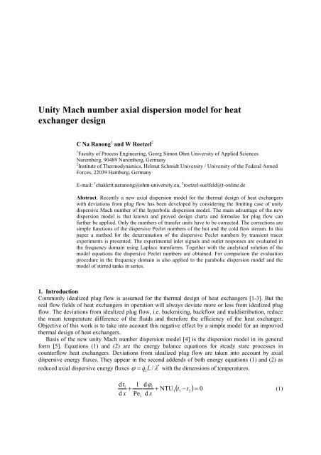
Unity Mach number axial dispersion model for heatexchanger designC Na Ranong 1 and W Roetzel 21 Faculty of Process Engineering, Georg Simon Ohm University of Applied SciencesNuremberg, 90489 Nuremberg, Germany2 Institute of Thermodynamics, Helmut Schmidt University / University of the Federal ArmedForces, 22039 Hamburg, GermanyE-mail: 1 chakkrit.naranong@ohm-university.eu, 2 roetzel-suelfeld@t-online.deAbstract. Recently a new axial dispersion model for the thermal design of heat exchangerswith deviations from plug flow has been developed by considering the limiting case of unitydispersive Mach number of the hyperbolic dispersion model. The main advantage of the newdispersion model is that known and proved design charts and formulae for plug flow canfurther be applied. Only the numbers of transfer units have to be corrected. The corrections aresimple functions of the dispersive Peclet numbers of the hot and the cold flow stream. In thispaper a method for the determination of the dispersive Peclet numbers by transient tracerexperiments is presented. The experimental inlet signals and outlet responses are evaluated inthe frequency domain using Laplace transforms. Together with the analytical solution of themodel equations the dispersive Peclet numbers are obtained. For comparison the evaluationprocedure in the frequency domain is also applied to the parabolic dispersion model and themodel of stirred tanks in series.1. IntroductionCommonly idealized plug flow is assumed for the thermal design of heat exchangers [1-3]. But thereal flow fields of heat exchangers in operation will always deviate more or less from idealized plugflow. The deviations from idealized plug flow, i.e. backmixing, backflow and maldistribution, reducethe mean temperature difference of the fluids and therefore the efficiency of the heat exchanger.Objective of this work is to take into account this negative effect by a simple model for an improvedthermal design of heat exchangers.Basis of the new unity Mach number dispersion model [4] is the dispersion model in its generalform [5]. Equations (1) and (2) are the energy balance equations for steady state processes incounterflow heat exchangers. Deviations from idealized plug flow are taken into account by axialdispersive energy fluxes. They appear in the second addends of both energy equations (1) and (2) as*reduced axial dispersive energy fluxes ϕ = L / λ with the dimensions of temperatures.q ldt1 dϕ1+ +1t1− td x Pe d xNTU ( ) 012=1(1)

dt2 1 dϕ2− + NTU2 1 2=d x Pe d x2( t − t ) 0(2)For the axial dispersive energy fluxes an empirical approach, equations (3) and (4), has beendeveloped on the basis of the hyperbolic heat conduction law [6, 7].2M1dϕ1d t1ϕ1+ = −(3)Pe d x d x12M2dϕ2dt2ϕ2− = −(4)Pe d x d x2The general hyperbolic dispersion model contains four parameters M 1 , M 2 , Pe 1 and Pe 2 , i.e. twodispersive Peclet numbers and two dispersive thermal Mach numbers [8 – 10]. The dispersive Pecletnumber is given byρcp*wLPe = . (5)λThe property λ * is an apparent thermal conductivity which is composed of the molecularconductivity and the convective dispersive contribution due to backflow, backmixing andmaldistribution. The molecular part is a fluid property and the convective one a flow property.Normally the molecular contribution is negligible.The dispersive thermal Mach number is given bywM = . (6)CFor pure convective phenomena of backflow, backmixing and maldistribution it can be expectedthat the propagation velocity of thermal disturbances C is in the order of the mean flow velocity w. Forpure molecular axial heat conduction according to Fourier’s law the propagation velocity of thermaldisturbances is infinite and M = 0. Table 1 shows the appropriate regions of application of the differentdispersion models with respect to the dispersive thermal Mach number, although all models can beapplied to arbitrary deviations from plug flow depending on the required accuracy [11 – 14].Table 1. Appropriate application of the dispersion models according to M.M type appropriate application0 parabolic axial heat conduction as in liquid metals0 < M < 1 hyperbolic pure backmixing and backflowM > 1 hyperbolic pure maldistribution in tube bundles or plate heat exchangers2. Unity Mach number dispersion modelThe analytical solution (M ≠ 1) even for the simple case of only one dispersive stream in acounterflow heat exchanger is very complicated and not suited for practical design calculations [9, 10].Thus a simplified less accurate model with a single fixed value of the thermal dispersive Mach numberis more appropriate. Since in industrial heat exchangers backmixing and backflow (M < 1) [9] as wellas maldistribution (M > 1) [9] takes place simultaneously, the value M = 1 seems to be a realistic mean

value which is at least better than M = 0 of the parabolic model. The special case M = 1 of thehyperbolic axial dispersion model is considered in the following. In equations (3) and (4) it becomesM 2 = 1.Figure 1. Temperature profiles in case of counterflow, NTU 1 =5, Pe 1 = 7, NTU 2 = 3, Pe 2 =10. NTU 1,d = 2.48 and NTU 2,d =1.49.To solve the governing equations (1) – (4) for the four dependent variables t 1 , t 2 , ϕ 1 and ϕ 2 onlytwo boundary conditions are necessary. The energy balance requires temperature jumps between thenon-dispersive region outside the heat exchanger and the dispersive region inside the heat exchanger(Figure 1). With given inlet temperatures of the fluids the two boundary conditions areT′=t11( x = 0)( x = 0)ϕ1+Pe1(7)andT′= t22( x = 1)ϕ2−Pe( x = 1)Finally, the outlet temperatures are calculated with exit conditions (9) and (10).2. (8)T′′=t21T′′=t21( x = 1)( x = 0)( x = 1)ϕ1+Pe1ϕ2−Pe( x = 0)2(9)(10)

3. Alternative formulation of the governing equationsThe main advantage of the new model becomes obvious if the governing equations (1) – (4) areformulated in an alternative way by introducing hypothetic temperatures T 1 (x) and T 2 (x) according toequations (11) and (12). The results are equations (13) and (14).ϕ1T1= t1+(11)Pe1ϕ2T2= t2−(12)Pe2dT1+ NTU1,d xdT2+ NTUd xd2, d( T −T)1= 0( T −T) = 0221(13)NTUiNTUi , d= , i = 1,2(14)NTU1NTU21++Pe Pe1Equation (13) has the mathematical form of the well-known energy equations of non-dispersiveplug flow. This means that known analytical solutions and design charts [1 – 3] can be used and thatthe dispersion effect can be accounted for solely by a correction of the number of transfer unitsaccording to equation (14). Figure 1 also shows the hypothetic temperatures which can be interpretedas the temperature profiles in an equivalent non-dispersive plug flow heat exchanger.Corresponding considerations [4] show that corrections (14) are also exactly valid for parallel flowand pure cross-flow. For other flow configurations the correction (14) yields sufficiently accurateapproximations [4]. The unity Mach number dispersion model has two parameters Pe 1 and Pe 2 . Itsapplication can be based on known plug flow solutions, diagrams and charts.4. Experimental determination of dispersive Peclet numbersTo apply the unity Mach number dispersion model, numerical values of dispersive Peclet numbersmust be available for the different types heat exchangers. In this paper a method which has beenoriginally applied to determine Peclet numbers of the parabolic dispersion model (M = 0) isconsidered [14] and transferred to the new model. The Peclet numbers of each flow side, e.g. shell sideand tube side of a shell and tube heat exchanger, can separately be determined by transient tracerexperiments. Taking the analogy between heat and mass transfer into account, the transient tracerexperiment corresponds to an adiabatic thermal experiment.4.1 Concept of adiabatic experimentsThe energy equation of a transient process in an adiabatic flow channel [9] with axial dispersion incase of M = 1 is∂t∂t+ = −∂z∂x1Pe2∂ϕ. (15)∂xIn principle, the energy equations (1) and (2) are on the one hand extended to allow for transient

process by the first addend of equation (15) and on the other hand they are simplified because NTU 1 =NTU 2 = 0 because the process is adiabatic. The index denoting the flow stream can be omitted sincethere is no interaction between the flow streams in this case.The empirical approach for the reduced axial dispersive energy flux [9] in case of M = 1 isϕ +1Pe⎛ ∂ϕ∂ϕ⎞ ∂t⎜ + ⎟ = − . (16)⎝ ∂z∂x⎠ ∂xAs for the steady state process the energy balance requires temperature jumps between the nondispersiveregion outside the heat exchanger and the dispersive region inside the heat exchanger. Atthe initial state the complete system has a uniform temperature which is normalized to zero and thereis no axial dispersive energy flux. The complete set of boundary and the initial conditions to solvepartial differential equations (15) and (16) isx = 0 :z = 0 :z = 0 :T′( x = 0, z) − t( x = 0, z) = ϕ( x = 0, z)Pet( x,z = 0)= 0ϕ( x,z = 0) = 01. (17)At the inlet the temperature T´´(z) may change arbitrarily with time. Common inlet signals are stepchange and Dirac pulse [13, 14]. The signal travels through the flow channel while it is changed due todispersion effects. The outlet signal of the process T´(z) is finally obtained from the exit condition1x = 1 : T′′( x = 1, z) = t( x = 1, z) + ϕ ( x = 1,z). (18)PeThe basic idea of the experiment is to calculate the dispersive Peclet number from measured inletand outlet signals. Because a simple analytic solution of equations (15) – (17) exists in the frequencydomain the dispersive Peclet number will be determined in the frequency domain from the Laplacetransforms of inlet and outlet signals.4.2. Determination of the dispersive Peclet number in the frequency domainIn the frequency domain the analytical relationship between inlet signal T´(z) und outlet signal T´´(z) isT ′′T ′( s)( s)⎛ Pe + s ⎞= exp ⎜−s ⎟ . (19)⎝ Pe + 2s⎠Equation (19) can be solved explicitly for the dispersive Peclet number:′′( s)′( s)( s)( s)Ts + 2lnTPe = −s(20)T ′′s + lnT ′If the inlet signals and outlet signals are known, the dispersive Peclet number can be directlycalculated. Since the dispersive Peclet number is a constant model parameter evaluation of equation(19) with arbitrary Laplace variables s must yield the same numerical of Pe, if the model exactly fits.

4.3 Evaluation procedureThe inlet and outlet signals can only be measured in the time domain. For the proposed method theyhave to be Laplace transformed into the frequency domain according toT∞∫z=0( s) T ( z) exp( − sz) dz= . (21)Figure 2. Example of inlet and outlet signals of an adiabatictransient experiments. Numerical integration according toequation (22) with denoted discrete measuring points.The experimental data will consist of a number of n equidistant discrete measuring points (figure2). Therefore, the integration according to equation (21) becomes a summation and the ratio betweenoutlet and inlet signal of equation (20) is approximatelyT ′′T ′( s)( s)≈1T′′1exp( −sz1)+21T′1exp( −sz1)+2n−1∑i=2n−1∑i=21T′′iexp( −szi)+ T′′nexp( −sz21T′iexp( −szi)+ T′nexp( −sz2nn). (22))Now equation (20) can be evaluated for different Laplace variables s. Since in general thedispersion model will not exactly fit, the dispersive Peclet number will not be the same for differentLaplace variables s, i.e.Pe = Pe(s) ≠ const. (23)For practical applications a mean dispersive Peclet number Pe m is proposed. Equation (24) requiresthe evaluation of equation (20) for four different values of s, table 2:

1Pem=23⎡ 1 1 ⎤ 1 ⎡ 1 1⎢ + ⎥ − ⎢ +⎢⎣Pe1 2Pe−1 2 ⎥⎦6 ⎣Pe+1Pe+ −1⎤⎥⎦(24)Table 2. Evaluation points for chosen value of s 1PesPe +1 s 1Pe +1/2 s 1 /2Pe -1/2 -s 1 /2Pe -1 -s 14.4 ExampleInstead of an adiabatic thermal experiment Balzereit [14] performed tracer experiments which areanalogous to adiabatic thermal experiments. The inlet signal is a Dirac pulse of concentration whichhas been realized with great experimental effort. The outlet signal for the shell side of a shell and tubeheat exchanger with 11 flow baffles is shown in figure 3.Figure 3. Experimental (•) and calculated (⎯) system responses to a Dirac pulse for the shell side of ashell and tube heat exchanger with 11 flow baffles; dimensionless outlet concentration as function ofdimensionless time: (a) unity Mach number dispersion model, (b) cascade model and (c) parabolicdispersion model.The evaluation procedure after section 4.3 yields a dispersive Peclet number Pe m = 38.6. For theparabolic dispersion model (M = 0) as in the original work of Balzereit [14] the dispersive Pecletnumber is 37.6, confirming the following relationship which can be derived from a comparison of bothmodels:(M=0) 2(M=1) [Pe ]Pe = (M=0)(M=0)Pe −1+exp[ −Pe](25)Finally, the heat exchanger can also be modeled as a cascade of stirred tanks in series [4]. Thetransfer function relating the outlet signal to the inlet signal in the frequency domain isT ′′T ′( s)1=( s) ( 1+s N ) N. (26)

In contrast to equation (19) the equation (26) cannot be solved explicitly for the model parameter ofinterest, i.e. the number of stirred tanks N. Data regression yields N = 19 for this example confirmingthe following relationship derived from steady state investigations and comparison between the unityMach number dispersion model and the stirred tank in series model:Pe (M=1) ≈ 2 N, (27)i.e. the Peclet number is directly proportional to the number of stirred tanks.For clarity the outlet responses of the different models are presented in the time domain afternumerical inversion of the Laplace transforms together with the experimental data in figure 3 showinggood agreement between model and experiment.5. Conclusions• The unity Mach number dispersion model allows a simple analytical solution of the energyequations for counterflow, parallel flow und pure cross-flow with dispersion on both flowsides.• For all flow configurations deviations from idealized plug flow can be taken into account bysimple corrections of the number of transfer units• All known analytical solutions and charts for idealized plug flow can be further used.• Peclet numbers can be determined for each flow side separately by tracer experiments.References[1] 2006 VDI-Wärmeatlas (Berlin: Springer)[2] 2010 Heat Atlas (Berlin: Springer)[3] Hewitt G, Shires G and Bott T 1994 Process heat transfer (Boca Raton: CRC Press)[4] Roetzel W, Na Ranong C and Fieg G 2011 New axial dispersion model for heat exchangerdesign Heat Mass Transf 47 (8) 1009-1017[5] Das S and Roetzel W 2004 The axial dispersion model for heat transfer equipment – A reviewInt J Transp Phenom 6 23 – 49[6] Chester M 1963 Second sound in solids. Phys Rev 131 2013 – 2015[7] Roetzel W, Spang B, Luo X and Das SK 1998 Propagation of the third sound wave in fluid:hypothesis and theoretical foundation Int J Heat Mass Transf 41 2769 - 2780[8] Roetzel W and Das S 1995 Hyperbolic axial dispersion model: Concept and its application to aplate heat exchanger Int J Heat Mass Transf 38 3065 – 3076[9] Roetzel W and Na Ranong C 2000 Axial dispersion models for heat exchangers Int J HeatTechnol 18 7 - 17[10] Sahoo R and Roetzel W 2002 Hyperbolic axial dispersion model for heat exchangers Int J HeatMass Transf 45 1261 - 1270[11] Spang B 1991 Über das thermische Verhalten von Rohrbündelwärmeübertragern mitSegmentumlenkblechen (VDI-Fortschrittsberichte, Reihe 19, Nr. 48)[12] Xuan Y 1991 Thermische Modellierung mehrgängiger Rohrbündelwärmeübertrager mitUmlenkblechen und geteiltem Mantelstrom (VDI-Fortschrittsberichte, Reihe 19, Nr. 52)(Düsseldorf: VDI)[13] Luo X 1998 Das axiale Dispersionsmodell für Kreuzstromwärmeübertrager (VDI-Fortschrittsberichte, Reihe 19, Nr. 109) (Düsseldorf: VDI)[14] Balzereit F 1999 Bestimmung von axialen Dispersionskoeffizienten in Wärmeübertragern ausVerweilzeitmessungen (VDI-Fortschrittsberichte, Reihe 19, Nr.120) (Düsseldorf: VDI)List of symbolscdimensionless concentration

C Propagation velocity of thermal disturbances (m s -1 )c p Specific isobaric heat capacity (J kg -1 K -1 )L Length of heat exchanger (m)l Space coordinate (m)M Dispersive thermal Mach number, M = w/CNTU Number of transfer unitsN number of stirred tanks in seriesn number of measuring pointsPe Dispersive Peclet number, Pe = w L ρ c p / λ*qlAxial dispersive energy flux (W m -2 )s Laplace variableT Hypothetic temperature (K)t Fluid temperature inside the exchanger (K)V Volume of fluid side (m 3 )V Volumetric flow rate (m 3 s -1 )w Mean flow velocity (m s -1 )x Dimensionless space coordinate (x = l/L)z Dimensionless time coordinate ( z = τ ( V/ V ) )Greek symbolsλ* apparent thermal conductivity (W m -1 K -1 )ϕ Reduced axial dispersive heat flux (K)ρ Density (kg m -3 )τ Time coordinate (s)Super- and subscriptsd dispersive1 Fluid 12 Fluid 2' Inlet'' Outlet- Laplace transform