Algorithm xxx: The Matlab Postprocessing Toolkit1 - Scott A. Sarra

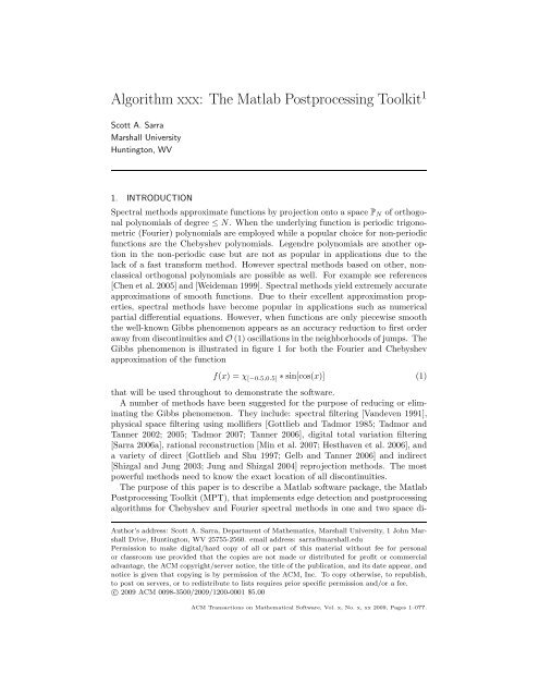
Algorithm xxx: The Matlab Postprocessing Toolkit 1Scott A. SarraMarshall UniversityHuntington, WV1. INTRODUCTIONSpectral methods approximate functions by projection onto a space P N of orthogonalpolynomials of degree ≤ N. When the underlying function is periodic trigonometric(Fourier) polynomials are employed while a popular choice for non-periodicfunctions are the Chebyshev polynomials. Legendre polynomials are another optionin the non-periodic case but are not as popular in applications due to thelack of a fast transform method. However spectral methods based on other, nonclassicalorthogonal polynomials are possible as well. For example see references[Chen et al. 2005] and [Weideman 1999]. Spectral methods yield extremely accurateapproximations of smooth functions. Due to their excellent approximation properties,spectral methods have become popular in applications such as numericalpartial differential equations. However, when functions are only piecewise smooththe well-known Gibbs phenomenon appears as an accuracy reduction to first orderaway from discontinuities and O (1) oscillations in the neighborhoods of jumps. TheGibbs phenomenon is illustrated in figure 1 for both the Fourier and Chebyshevapproximation of the functionf(x) = χ [−0.5,0.5] ∗ sin[cos(x)] (1)that will be used throughout to demonstrate the software.A number of methods have been suggested for the purpose of reducing or eliminatingthe Gibbs phenomenon. They include: spectral filtering [Vandeven 1991],physical space filtering using mollifiers [Gottlieb and Tadmor 1985; Tadmor andTanner 2002; 2005; Tadmor 2007; Tanner 2006], digital total variation filtering[Sarra 2006a], rational reconstruction [Min et al. 2007; Hesthaven et al. 2006], anda variety of direct [Gottlieb and Shu 1997; Gelb and Tanner 2006] and indirect[Shizgal and Jung 2003; Jung and Shizgal 2004] reprojection methods. The mostpowerful methods need to know the exact location of all discontinuities.The purpose of this paper is to describe a Matlab software package, the MatlabPostprocessing Toolkit (MPT), that implements edge detection and postprocessingalgorithms for Chebyshev and Fourier spectral methods in one and two space di-Author’s address: Scott A. Sarra, Department of Mathematics, Marshall University, 1 John MarshallDrive, Huntington, WV 25755-2560. email address: sarra@marshall.eduPermission to make digital/hard copy of all or part of this material without fee for personalor classroom use provided that the copies are not made or distributed for profit or commercialadvantage, the ACM copyright/server notice, the title of the publication, and its date appear, andnotice is given that copying is by permission of the ACM, Inc. To copy otherwise, to republish,to post on servers, or to redistribute to lists requires prior specific permission and/or a fee.c○ 2009 ACM 0098-3500/2009/1200-0001 $5.00ACM Transactions on Mathematical Software, Vol. x, No. x, xx 2009, Pages 1–0??.

2 · Scott A. Sarramensions. The software is intended for applications, algorithm benchmarking, andeducational purposes. The MPT is a significant extension and translation of theSpectral Signal Processing Suite (SSPS) [Sarra 2003c]. The SSPS was implementedin the Java programming language which limited its usefulness. The SSPS only implementededge detection, spectral filtering, and Gegenbauer Reprojection, for onedimensional Chebyshev approximations. The MPT is implemented in a languageknown by a large number of scientists and engineers and is broader in the scope ofalgorithms implemented. Details of the available user callable M-files along witha selection of example problems and associated results may be found in the usermanual distributed with the software.0.9Fourier0.9Chebyshev0.80.80.70.70.60.60.50.5f(x)0.4f(x)0.40.30.30.20.20.10.100−0.1−1 −0.5 0 0.5 1x−0.1−1 −0.5 0 0.5 1xFig. 1. Spectral approximation of function (1) vs. the exact function. The function is known atN = 200 interpolation sites and the interpolant is evaluated at M = 298 evenly spaced points.Left: Fourier. Right: Chebyshev.2. GLOBAL POLYNOMIAL APPROXIMATION METHODSThe software package is based on interpolation, rather than expansion, methodsincorporating Chebyshev and trigonometric polynomials. Interpolation and expansionmethods have the same excellent approximation properties but we have choseninterpolation since pseudospectral methods for PDEs are based on interpolation.The interpolating approximationI N f(x) = ∑ ka k φ k (x) (2)with expansion coefficients a k and basis functions φ k (x) on interval Ω = [−1, 1],satisfies I N f(x i ) = f(x i ) at N + 1 interpolation sites x i . Interpolation meansthat f(x), the function that is approximated, is a known function (at least at theinterpolation sites) while the terms collocation and pseudospectral are applied toglobal polynomial interpolatory methods for solving differential equations for anunknown function f(x). We refer to both situations as spectral approximation orACM Transactions on Mathematical Software, Vol. x, No. x, xx 2009.

The Matlab Postprocessing Toolkit · 3spectral methods. Detailed information on spectral methods may be found in thestandard references [Boyd 2000; Canuto et al. 2006; Hesthaven et al. 2007; Reyret2002; Trefethen 2000].2.1 Chebyshev InterpolationIn (2) the index k runs over k = 0, 1, . . .,N and the basis functions are the Chebyshevpolynomials [Mason and Handscomb 2003]φ k (x) = T k (x) = cos(k arccos(x)). (3)The expansion coefficients are efficiently calculated via the FFT (chebyshevCoefficients.m).The interpolation sites are the Chebyshev-Gauss-Lobatto (CGL) points( ) kπx k = − cos k = 0, 1, . . .,N. (4)NThe CGL points are the locations of the N −1 extrema of T N (x) plus the endpointsof the interval [−1, 1].2.2 Fourier (Trigonometric) InterpolationThe degree 2N Fourier approximation method uses evenly spaced interpolationsitesx k = −1 + 2 k, k = 0, 1, . . .,N − 1 (5)Non [−1, 1]. In (2) the index k runs over k = −N, −N + 1, . . .,N and the basisfunctions are the trigonometric polynomialsφ k (x) = e ikπx . (6)The expansion coefficients are efficiently calculated via the FFT.3. EDGE DETECTIONThe majority of postprocessing algorithms either require or may incorporate theexact location of discontinuities, or edges, in the function. Edge detection methodshave been developed in references [Gelb and Tadmor 1999; 2000a]. Twochoices of concentration factors are available in the edge detection routines, alinear concentration factor of σ(ξ) = ξ and an exponential concentration factor1σ(ξ) = ξ exp(6ξ(ξ−1)). Details on concentration factors can be found in references[Gelb and Tadmor 1999] and [Gelb and Tadmor 2000a].The edges are located by examining a weighted derivative of the spectral interpolantue(x) = w ddx I Nf(x) (7)where the weight is w = 1/N in the Fourier case and w = π √ 1 − x 2 /N for theChebyshev case. Denoting the location of discontinuities as α j and defining jumpsas[f](x) := f(x + ) − f(x − )ACM Transactions on Mathematical Software, Vol. x, No. x, xx 2009.

4 · Scott A. Sarrathe convergence of ue(x) to the location of the discontinuities may be described as{ (O1)ue(x) → N when x ≠ αj[f] (α j ) when x = α j .While a graphical examination of ue(x) verifies that it does have the desired convergenceproperties, an additional step is needed to numerically pinpoint the locationof the discontinuities. For that purpose, a non-linear enhancement [Gelb and Tadmor2000a] is made to ue(x) asun(x) = N Q 2 [ue(x)] Q .The enhanced sum has the convergence properties{ ( )O N −Q 2 when x ≠ α jun(x) →N Q 2 [[f] (α j )] Q when x = α j .By choosing Q > 1, the separation is enhanced between the O([ 1 N ] Q 2 ) points ofsmoothness and the O(N Q 2 ) points of discontinuity. The problem dependent thresholdparameter J is then used to pinpoint the location of all jumps and the edgesare located by redefining ue(x) as{ ue(x) if |un(x)| > Jue(x) =0 otherwise.Computational experience [Sarra 2003c] has lead to the inclusion of an additionalparameter η which controls the number of edges that can be found in the neighborhoodof a local maximum of ue(x). If the maximum occurs at x(i), then theparameter allows only one edge to be found in the interval (x[i − η], x[i + η]),i = 0, ..., N.The edge detection procedure can be employed repeatedly to find discontinuitiesin the l th derivative of a function and to determine intervals of C l -smoothness. Forexample, to find the discontinuities in the first derivative, first the locations of thediscontinuities in the function are found. Then in each smooth subinterval, I N f(x)is differentiated and the edge detection procedure is applied to find the jumps inthe first derivative. An example describing edge detection in a function and its firstderivative can be found in reference [Gelb and Tadmor 2000b].4. POSTPROCESSING METHODS4.1 Spectral FiltersSpectral filters [Vandeven 1991] lessen the effects of the Gibbs phenomenon byworking in transform space asF N f(x) = ∑ kσ(k/N)a k φ k (x) (8)The convergence rate of the filtered approximation is determined solely by theorder, ρ > 1, of the filter and the regularity of the function away from the pointof discontinuity. If the filter order, ρ, is chosen increasing with N, the filteredACM Transactions on Mathematical Software, Vol. x, No. x, xx 2009.

The Matlab Postprocessing Toolkit · 5expansion recovers exponential accuracy away from a discontinuity. Assuming thatf(x) has a discontinuity at x 0 and setting d(x) = x − x 0 , the estimate|f(x) − F N (x)| ≤Kd(x) ρ−1 N ρ−1 (9)holds where K is a constant. If ρ is sufficiently large, and d(x) is not too small,the error goes to zero faster than any finite power of N, i.e. spectral accuracy isrecovered. When x is close to a discontinuity the error increases. If d(x) = O(1/N)then the error estimate is O(1).The following ρ th order spectral filters are implemented in the MPT:(1) exponential filterσ 1 (ω) = e (ln εm) ωρ , (10)where ρ even and ε m represents machine zero.(2) Erfc-Log filter [Boyd 1996]√)σ 2 (ω) =(2 1 2 erfc √ − ln (1 − 4 [|ω| − 1/2] 2 )ρ [|ω| − 1/2]4 [|ω| − 1/2] 2(3) Vandeven filter [Vandeven 1991]σ 3 (ω) = 1 −4.2 Digital Total Variation Filtering(2ρ − 1)!(p − 1)!∫ |ω|0(11)t ρ−1 (1 − t) ρ−1 dt. (12)The Rudin, Osher, and Fatemi (ROF) Total Variation (TV) denoising model is apopular image processing method to remove noise from a digital image. The modelformulates a minimization problem which leads to a nonlinear Euler-Lagrange PDEto be solved by numerical PDE methods. In [Chan et al. 2001; Osher and Shen 2000]the authors develop a discrete version of the TV model on a graph - Digital TotalVariation (DTV) filtering. Viewing an oscillatory function as an image with noise,the DTV method was used to postprocess spectral approximations in [Sarra 2006a]and Radial Basis Function approximations in [Sarra 2006b]. The method works withpoint values in physical space and not with the spectral expansion coefficients. TheDTV method does not need to know the location of edges. The point values maybe located at scattered, non-structured sites, in complex geometries. The DTVmethod is very computationally efficient. While the method does mitigate theeffects of the Gibbs phenomenon it does not make any claims of restoring spectralaccuracy.To summarize the method, let [Ω, G] be a finite set Ω of nodes and a dictionaryof edges G connecting the nodes. General vertices are denoted by α, β, · · · . Thenotation α ∼ β indicates that α and β are linked by an edge. All the neighbors ofα are denoted byN α = {β ∈ Ω | β ∼ α}. (13)The graph variational problem is to minimize the fitted TV energyEλTV (u) = ∑ |∇ α u| a+ λ ∑(u α − u 02α) 2 (14)α∈Ωα∈ΩACM Transactions on Mathematical Software, Vol. x, No. x, xx 2009.

6 · Scott A. Sarrawhere u 0 is the spectral approximation containing the Gibbs oscillations and λ theuser specified fitting parameter. The unique solution to this problem is the solutionof the nonlinear restoration equation∑(u α − u β )β∼α( 1|∇ α u| a+)1+ λ(u α − u 0 α|∇ β u| ) = 0 (15)awhere the regularized location variation or strength function at any node α isdefined as⎡|∇ α u| a= ⎣ ∑1/2⎦ . (16)β∈N α(u β − u α ) 2 + a 2 ⎤The regularization parameter a is a small (the default in the software is a = 0.0001)value used to prevent a zero local variation and division by zero.The nonlinear system can be solved by a linearized Jacobi iteration as was donein [Chan et al. 2001; Sarra 2006a; 2006b]. Alternatively, we can work with thenonlinear restoration equation (15) and use time marching to reach a steady statedu αdt= ∑ β∼α(u α − u β )Preconditioning equation (17)du αdt= ∑ β∼α(u α − u β )( 1|∇ α u| a+)1+ λ(u α − u 0 α ). (17)|∇ β u| a(1 + |∇ )αu| a+ λ |∇ α u||∇ β u| a(u α − u 0 α ). (18)ayields a faster convergence to the steady state [Osher and Shen 2000]. The softwareuses time marching with the explicit Euler’s method. Typically about 100 time stepsare required to approach a steady state. An optimal value of the fitting parameterλ is not known. However, a large range of values for the fitting parameter resultsin a “good” postprocessing. In general, stronger oscillations are best handled witha small fitting parameter (< 10) while weaker oscillations require a larger value ofthe fitting parameter. More details on selecting the value of the shape parametercan be found in references [Sarra 2006a] and [Sarra 2009].In two space dimensions there is more than one way to define N α (figure 2). Oneis to consider at a node α i,j four neighboring points,N 4 α = {α i,j+1, α i+1,j , α i,j−1 , α i−1,j }and another is an eight point neighborhood,N 8 α = {α i,j+1 , α i+1,j+1 , α i+1,j , α i+1,j−1 , α i,j−1 , α i−1,j−1 , α i−1,j , α i−1,j+1 }.4.3 Rational ReconstructionRational functions have been used in several different forms to reduce the Gibbsphenomenon [Clenshaw and Lord 1974; Driscoll and Fornberg 2001; Hesthaven andKaber 2008; Hesthaven et al. 2006; Min et al. 2007]. Rational functions are morecomplex than simple polynomials and often do better in approximation discontinuousfunctions or functions with steep gradients.ACM Transactions on Mathematical Software, Vol. x, No. x, xx 2009.

The Matlab Postprocessing Toolkit · 7(i,j+1)(i−1,j+1)(i,j+1)(i+1,j+1)(i−1,j) (i,j)(i+1,j) (i−1,j)(i,j)(i+1,j)(i,j−1)(i−1,j−1)(i,j−1)(i+1,j−1)Fig. 2.2d DTV neighborhoods: Left, N 4 α . Right: N8 αA Padé approximant is of the formR K,M = P KQ M=∑ Kk=0 p kφ k (x)∑ Mm=0 q mφ m (x)(19)The linear Padé approximation of a function u is determined by imposing theorthogonality relations〈Q M u − P K , φ〉 = 0, ∀φ ∈ P N (20)From this, a linear system with M + 1 unknowns and K − N equations can beextracted. Reference [Hesthaven and Kaber 2008] can be consulted for details.After the degree of the denominator M is chosen the degree of the numeratoris set as K = (N − N c ) − M where N c

8 · Scott A. Sarrai smooth subintervals [a, b] the function is reprojected as∑m ifP(x) i = glΨ i l [ξ(x)] (21)l=0onto a basis Ψ l (x) of polynomials, the reprojection basis, which are orthogonal on[−1, 1] with respect to a weight function w(x) under the weighted inner product(Ψ k (ξ), Ψ k (ξ)) w which satisfies(Ψ k (ξ), Ψ l (ξ)) w =∫ 1−1Ψ k (ξ)Ψ l (ξ)w(ξ)dξ = γ l δ kl (22)where γ l is a normalization factor. The expansion coefficients gl i are evaluatedvia a Gaussian quadrature formula. If the function being approximated is knownat the quadrature points, gl i are referred to as the exact reprojection coefficients.Otherwise the spectral interpolant (2) is used to approximate the function at thequadrature points and the coefficients are referred to as the approximate reprojectioncoefficients ĝl i.The accuracy of the reprojection methods depends on accurately locating alldiscontinuities and intervals of smoothness. Failure to identify a discontinuity willcause the methods to fail badly. However, the methods are fairly robust to misidentifyingthe location of a discontinuity within a cell or two. This is because the weightof the reprojection basis tapers smoothly to zero at its boundaries and the reprojectioncoefficients are computed by multiplying the original function or its spectralprojection by the reprojection weight. In the neighborhood of discontinuities, theresult of the multiplication is very small if the weight is properly designed andcrossing a discontinuity by a few cells will only result in a correspondingly smallerror.4.4.1 Gegenbauer Reprojection. The Gegenbauer Reprojection Procedure (GRP)uses the Gegenbauer or Ultraspherical polynomials C λ las the reprojection basis.The GRP was developed in the series of papers [Gottlieb et al. 1992; Gottlieb andShu 1994; 1996; 1995a; 1995b; 1997]. Further analysis and application of the GRPcan be found in references [Boyd ; Jackiewicz 2003; Sarra 2003a; 2003b]. Reference[Boyd ] describes how the convergence of the GRP is adversely affected when theunderlying function has singularities off the real axis.The Gegenbauer polynomials satisfy the conditions of a Gibbs complementarybasis [Hesthaven et al. 2007] which allows for a spectrally accurate reprojection.The weight function associated with the Gegenbauer polynomials is w(x) = (1 −ξ 2 ) λ−1/2 . The Gegenbauer polynomials (gegenbauerPolynomial.m) are calculatedvia the three term recurrence relationC λ k+1(ξ) =2(k + λ)ξk + 1Ck λ (ξ) − k + 2λ − 1 C λk + 1k−1(ξ), k = 1, 2, . . . (23)with C λ 0 = 1 and C λ 1 = 2λξ.In smooth subinterval i the GRP postprocessed approximation ism ifP i (x) = ∑l=0g i l Cλ lACM Transactions on Mathematical Software, Vol. x, No. x, xx 2009.[ξ(x)] (24)

where the exact Gegenbauer expansion coefficients areandg i l = 1γ λ l∫ 1−1γ λ l = π 1 2The Matlab Postprocessing Toolkit · 9(1 − ξ 2 ) λ−1/2 C λ l (ξ)f[x(ξ)]dξ (25)Γ(l + 2λ)Γ(λ + 1 2 )l!Γ(2λ)Γ(λ)(n + λ) .If only the expansion coefficients a k are known and not the underlying function, asin a pseudospectral PDE approximation, the Gegenbauer coefficients are replacedwith the approximate Gegenbauer coefficientsĝ i l = 1γ λ l∫ 1−1(1 − ξ 2 ) λ−1/2 C λ l (ξ)I Nf[x(ξ)]dξ. (26)The integrals in (25) and (26) are evaluated via Chebyshev-Gauss-Lobatto quadrature.4.4.2 Freud Reprojection. The Freud Reprojection Procedure (FRP) [Gelb 2007;Gelb and Tanner 2006] uses the Freud polynomials ψ as the reprojection basis andthe weight function is w(ξ) = e −cξ2λ where λ = αN, 0 ( < α < 1, and c = lnǫ √N(b √ M )where ǫ M is machine epsilon. We have used λ = round − a)/2 − 2 (2)which was suggested in [Gelb and Tanner 2006].In [Gelb and Tanner 2006] an additional condition is added to the three conditionsthat a Gibbs complementary basis must satisfy. A basis that satisfies the fourconditions is called a Robust Gibbs complement. The Freud polynomial basis is anexample of a Robust Gibbs complement. Freud reprojection does not suffer fromthe numerical roundoff errors and the Runge phenomenon that the GRP does [Boyd]. The Freud polynomials are not known explicitly but can be computed recursivelyasψ k+1 (ξ) = ξψ k (ξ) −γ kψ k−1 (ξ)γ k−1where ψ 0 (ξ) = 1 and ψ 1 (ξ) = ξ. The recursion coefficients areγ k = (ψ k (ξ), ψ k (ξ)) w =The exact Freud coefficients areand the approximate Freud coefficients are∫ 1−1ψ k (ξ)ψ k (ξ)e −cξ2λ dξ. (27)gl i = 1 ∫ −1e −cξ2λ ψ l (ξ)f[x(ξ)]dξ. (28)γ l1ĝl i = 1 ∫ −1e −cξ2λ ψ l (ξ)I N f[x(ξ)]dξ. (29)γ l1Integrals (27), (28), and (29) are evaluated very accurately using the trapezoidrule which is exponentially accurate for smooth periodic functions. In smoothACM Transactions on Mathematical Software, Vol. x, No. x, xx 2009.

10 · Scott A. Sarrasubinterval i the FRP approximation is∑m ifP(x) i = glψ i l [ξ(x)]. (30)l=0In each subinterval of smoothness m i is set m i = N(b − a)/8. However, as N increasesthe number of terms in the reprojection basis m i is more than is necessary tonumerically resolve the function and the higher numbered reprojection coefficientsbecome very close to machine epsilon which leads to round-off errors. As describedon p. 15 of [Gelb and Tanner 2006], the round-off errors can be avoided by resettingm i to a value that prevents the average of three consecutive reprojectioncoefficients from being larger than a specified tolerance. Experimentally we havefound a tolerance of 10e-12 to work well in the Fourier case and 10e-8 to work wellwith Chebyshev approximations.For the FRP, the specification of M is not function-dependent as is the case forthe GRP. The FRP does not have any function-dependent parameters to be suppliedby the user. This is in contrast to the GRP which depends heavily on the properspecification of both a weight parameter λ and reprojection order M. Numericalevidence indicates that the FRP recovers exponential accuracy. However, due tothe incomplete knowledge of the Freud polynomials, this result has not been provento hold.4.4.3 Inverse Reprojection. The Gegenbauer and Freud reprojection methodsare referred to as direct methods as they compute the reprojection coefficientsdirectly from the spectral expansion coefficients a k (or function values). In contrast,inverse methods compute the reprojection coefficients by solving a linear system ofequationsWg = a.The Inverse Reprojection method was developed in [Jung and Shizgal 2004; 2005;Shizgal and Jung 2003]. A recent application of the Inverse Reprojection method totime-dependent PDE solutions can be found in [Abdi and Hosseini 2008]. Originally[Shizgal and Jung 2003], the Gegenbauer polynomials were used as the reprojectionbasis, but later [Jung and Shizgal 2004; 2005] the method was generalized to yielda unique reconstruction using any set of basis functions. The generalized methodis referred to as the inverse polynomial reconstruction method (IPRM).We have implemented the method using the Gegenbauer polynomials as the reconstructionbasis. Note that since the IPRM uniquely determines the reconstructionfor any reconstruction basis, the Gegenbauer parameter λ does not play a rolein the method as it does in the GRP method. The matrix W may be very illconditioned.This problem is addressed in reference [Jung and Shizgal 2007]. Theconditioning of W is best for small λ > 0 [Shizgal and Jung 2003]. In the computercode the default is λ = 1/2 which corresponds to the Legendre basis. Care has beentaken to consistently evaluate the spectral expansion coefficients and the integralsthat determine the elements of the matrix W as is discussed in [Jung and Shizgal2004]. Both are evaluated using Gaussian quadrature.ACM Transactions on Mathematical Software, Vol. x, No. x, xx 2009.

5. GRAPHICAL USER INTERFACEThe Matlab Postprocessing Toolkit · 11The Matlab functions of the MPT may be called directly from user written Matlabcode as we have illustrated in the examples provided in the user manual that accompaniesthe software. Additionally, to make the MPT functions more accessibleto non-Matlab users a graphical user interface (GUI) has been developed. TheGUI has built-in functions and pseudospectral PDE solutions that can be used todemonstrate and benchmark the algorithms. The Fourier PDE examples includelinear advection and inviscid Burger’s equation and the Chebyshev examples includelinear advection and the Euler equations of gas dynamics. More details of theGUI may be found in the GUI user guide which is also include with the distributedsoftware. A screen shot of the GUI is shown in figure 3.Fig. 3. Graphical user interface6. CONCLUDING COMMENTSWe have described a suite of Matlab programs that implement state-of-the-artpostprocessing and edge detection algorithms for Fourier and Chebyshev spectralapproximations of piecewise smooth functions in one and two space dimensions.ACM Transactions on Mathematical Software, Vol. x, No. x, xx 2009.

12 · Scott A. SarraPostprocessing methods that require one or more user defined parameters be specifiedin each smooth subregion are difficult to implement in two space dimensions.For this reason, the MPT only implements spectral filtering and DTV filtering intwo dimensions. Although not the most powerful one dimensional methods, theyare very computationally efficient and the closest to “black box” algorithms in twodimensions. In two dimensional applications, many of the one dimensional methodscan been applied to one dimensional slices in the x or y direction. This approachhas been taken in references [Jung and Shizgal 2005] and [Min et al. 2007].The MPT functions may be called directly from a Matlab script. Alternatively,the routines may be accessed from a GUI. The postprocessing functions and accompanyingGUI with built-in example functions and PDE solutions provide usersthe opportunity to benchmarch and demonstrate the postprocessing algorithms.Experienced Matlab users will find it easy to modify the GUI to incorporate theirown algorithms or example problems. The development of the MPT is ongoing andmodifications and extensions will be made as new algorithms are developed.We conclude with table 6 that summarizes the basic feature of the postprocessingalgorithms.edge spectral largemethod detection parameters accuracy κ(A)spectral filter ρ ∼DTVλ√Padé√∼ M, N c√GRP√λ, m i√FRP∗√√ √IPRMm iA √ in the edge detection column indicates the method must know the exact locationof the discontinuities while a ∼ indicates that the edge location may beincorporated to improve the method. The parameters column lists any user specifiedparameters. If the method incorporates edge detection the parameters must bespecified in each subinterval of smoothness. A √ in the spectral accuracy columnindicates the method is able to recover spectral accuracy over the entire intervalwhile a ∼ indicates that spectral accuracy may be recovered over a portion of theinterval sufficiently away from the edge locations. The √∗ in the spectral accuracycolumn of the FRP indicates numerically observed but not theoretical proven spectralaccuracy. A √ in the large κ(A) column indicates that a linear system must besolved to implement the method and that the matrix may have a large conditionnumber.REFERENCESAbdi, A. and Hosseini, S. M. 2008. An investigation of resolution of 2-variate Gibbs phenomenon.Applied Mathematics and Computation 203, 714–732.Boyd, J. P. Trouble with Gegenbauer reconstruction for defeating Gibbs’ phenomenon: Rungephenomenon in the diagonal limit of Gegenbauer polynomial approximations. Journal of ComputationalPhysics.Boyd, J. P. 1996. The Erfc-Log filter and the asymptotics of the Vandeven and Euler sequenceaccelerations. Houston Journal of Mathematics, 267–275.Boyd, J. P. 2000. Chebyshev and Fourier Spectral Methods, second ed. Dover.ACM Transactions on Mathematical Software, Vol. x, No. x, xx 2009.

The Matlab Postprocessing Toolkit · 13Canuto, C., Hussaini, M., Quarteroni, A., and Zang, T. 2006. Spectral Methods: Fundamentalsin Single Domains. Springer.Chan, T., Osher, S., and Shen, J. 2001. The digital TV filter and nonlinear denoising. IEEETransactions on Image Processing 10, 2.Chen, Q., Gottlieb, D., and Hesthaven, J. 2005. Spectral methods based on prolate spheroidalwave functions for hyperbolic PDEs. SIAM Journal on Numerical Analysis 43, 5, 1912–1933.Clenshaw, C. W. and Lord, K. 1974. Rational approximations from Chebyshev series. InStudies in Numerical Analysis, B. Scaife, Ed. Academic Press, 95113.Driscoll, T. and Fornberg, B. 2001. A Padé-based algorithm for overcoming the Gibbs phenomenon.Numerical Algorithms 26, 77–92.Gelb, A. 2007. Reconstruction of piecewise smooth functions from non-uniform grid data. Journalos Scientific Computing 30, 3, 409–440.Gelb, A. and Tadmor, E. 1999. Detection of edges in spectral data. Applied and ComputationalHarmonic Analysis 7, 101–135.Gelb, A. and Tadmor, E. 2000a. Detection of edges in spectral data II: Nonlinear enhancement.SIAM Journal of Numerical Analysis 38, 4, 1389–1408.Gelb, A. and Tadmor, E. 2000b. Enhanced spectral viscosity approximations for conservationlaws. Applied Numerical Mathematics 33, 3–21.Gelb, A. and Tanner, J. 2006. Robust reprojection methods for the resolution of the Gibbsphenomenon. Applied and Computational Harmonic Analysis 20, 3–25.Gottlieb, D. and Shu, C.-W. 1994. Resolution properties of the Fourier method for discontinuouswaves. Comput. Methods Appl. Mech. Engrg. 116, 27–37.Gottlieb, D. and Shu, C.-W. 1995a. On the Gibbs phenomenon IV: Recovering exponentialaccuracy in a subinterval from a Gegenbauer partial sum of a piecewise analytic function.Mathematics of Computation 64, 1081–1095.Gottlieb, D. and Shu, C.-W. 1995b. On the Gibbs phenomenon V: Recovering exponential accuracyfrom collocation point values of a piecewise analytic function. Numerische Mathematik 71,511–526.Gottlieb, D. and Shu, C.-W. 1996. On the Gibbs phenomenon III: Recovering exponentialaccuracy in a subinterval from a partial sum of a piecewise analytic function. SIAM Journalof Numerical Analysis 33, 280–290.Gottlieb, D. and Shu, C.-W. 1997. On the Gibbs phenomenon and its resolution. SIAMReview 39, 4, 644–668.Gottlieb, D., Shu, C.-W., Solomonoff, A., and Vandeven, H. 1992. On the Gibbs phenomenonI: recovering exponential accuracy from the Fourier partial sum of a nonperiodicanalytic function. Journal of Computational and Applied Mathematics 43, 81–98.Gottlieb, D. and Tadmor, E. 1985. Recovering pointwise values of discontinuous data withinspectral accuracy. In Progress and Supercomputing in Computational Fluid Dynamics, E. M.Murman and S. S. Abarbanel, Eds. Birkhäuser, Boston, 357–375.Hesthaven, J., Gottlieb, S., and Gottlieb, D. 2007. Spectral Methods for Time-DependentProblems. Cambridge University Press.Hesthaven, J. and Kaber, S. 2008. Padé-Jacobi approximants. Under Review. Journal ofComputational and Applied Mathematics.Hesthaven, J., Kaber, S., and Lurati, L. 2006. Padé-Legendre interpolants for Gibbs reconstruction.Journal of Scientific Computing 28, 2-3, 337–359.Jackiewicz, Z. 2003. Determination of optimal parameters for the Chebyshev-Gegenbauer reconstructionmethod. SIAM Journal of Scientific Computing 25, 4.Jung, J.-H. and Shizgal, B. 2004. Generalization of the inverse polynomial reconstructionmethod in the resolution of the Gibbs phenomenon. Journal of Computational and AppliedMathematics 172, 131–151.Jung, J.-H. and Shizgal, B. 2005. Inverse Polynomial Reconstruction of Two DimensionalFourier Images. Journal of Scientific Computing 25, 367–399.ACM Transactions on Mathematical Software, Vol. x, No. x, xx 2009.

14 · Scott A. SarraJung, J.-H. and Shizgal, B. 2007. On the numerical convergence with the inverse polynomialreconstruction method for the resolution of the Gibbs phenomenon. Journal of ComputationalPhysics 224, 477–488.Mason, J. and Handscomb, D. 2003. Chebyshev Polynomials. CRC.Min, M. S., Kaber, S. M., and Don, W. S. 2007. Fourier-Padé approximations and filteringfor spectral simulations of an incompressible Boussinesq convection problem. Mathematics ofComputation 76, 1275–1290.Osher, S. and Shen, J. 2000. Digitized PDE method for data restoration. In Analytic-Computational Methods in Applied Mathematics, G. Anastassiou, Ed. Chapman and Hall/CRC,Chapter 16, 751–771.Reyret, R. 2002. Spectral Methods for Incompressible Viscous Flow. Springer.Sarra, S. A. 2003a. Chebyshev super spectral viscosity method for a fluidized bed model. Journalof Computation Physics 186, 2, 630–651.Sarra, S. A. 2003b. Spectral methods with postprocessing for numerical hyperbolic heat transfer.Numerical Heat Transfer 43, 7, 717–730.Sarra, S. A. 2003c. The spectral signal processing suite. ACM Transactions on MathematicalSoftware 29, 2.Sarra, S. A. 2006a. Digital Total Variation filtering as postprocessing for Chebyshev pseudospectralmethods for conservation laws. Numerical Algorithms 41, 17–33.Sarra, S. A. 2006b. Digital Total Variation filtering as postprocessing for Radial Basis FunctionApproximation Methods. Computers and Mathematics with Applications 52, 1119–1130.Sarra, S. A. 2009. Edge detection free postprocessing for pseudospectral approximations. Toappear in the Journal of Scientific Computing.Shizgal, B. and Jung, J.-H. 2003. Towards the resolution of the Gibbs phenomena. Journal ofComputational and Applied Mathematics 161, 41–65.Tadmor, E. 2007. Filters, mollifiers and the computation of the Gibbs phenomenon. ActaNumerica 16, 305–378.Tadmor, E. and Tanner, J. 2002. Adaptive mollifers - high resolution recovery of piecewisesmooth data from its spectral information. Foundations of Computational Mathematics 2,155–189.Tadmor, E. and Tanner, J. 2005. Adaptive filters for piecewise smooth spectral data. IMAJournal of Numerical Analysis 25, 4.Tanner, J. 2006. Optimal filter and mollifier for piecewise smooth spectral data. Mathematicsof Computation 75, 254.Trefethen, L. N. 2000. Spectral Methods in Matlab. SIAM, Philadelphia.Vandeven, H. 1991. Family of spectral filters for discontinuous problems. SIAM Journal ofScientific Computing 6, 159–192.Weideman, J. 1999. Spectral methods based on nonclassical orthogonal polynomials. InternationalSeries of Numerical Mathematics 31, 239–251.ACM Transactions on Mathematical Software, Vol. x, No. x, xx 2009.