quantum electrodynamics - quantresearch.info

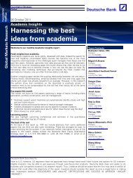
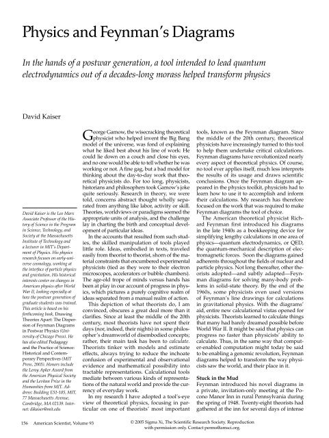
Santa Barbara News-PressFigure 1. Feynman diagrams were invented in 1948 to help physicists find their way out of a morass of calculations troubling a field of theorycalled QED, or quantum electrodynamics. Since then, they have filled blackboards around the world as essential bookkeeping devices in thecalculation-rich realm of theoretical physics. Here David Gross (center), in a newspaper photograph taken shortly after he was awarded the2004 Nobel Prize in Physics with H. David Politzer and Frank Wilczek, uses a diagram to discuss recent results in perturbative QCD (quantumchromodynamics) motivated by string theory with 1999 Nobelist Gerardus ’t Hooft (facing Gross at far right) and postdoctoral researchers MichaelHaack and Marcus Berg at the University of California, Santa Barbara. Gross, Politzer and Wilczek’s 1973 discovery paved the way forphysicists to use the diagrams successfully in QCD.discussions. Most of the young theorists werepreoccupied with the problems of QED. Andthose problems were, in the understated languageof physics, nontrivial.QED explains the force of electromagnetism—thephysical force that causes like chargesto repel each other and opposite charges toattract—at the quantum-mechanical level. InQED, electrons and other fundamental particlesexchange virtual photons—ghostlikeparticles of light—which serve as carriers ofthis force. A virtual particle is one that has borrowedenergy from the vacuum, briefly shimmeringinto existence literally from nothing.Virtual particles must pay back the borrowedenergy quickly, popping out of existence again,on a time scale set by Werner Heisenberg’s uncertaintyprinciple.Two terrific problems marred physicists’ effortsto make QED calculations. First, as theyhad known since the early 1930s, QED producedunphysical infinities, rather than finiteanswers, when pushed beyond its simplestapproximations. When posing what seemedlike straightforward questions—for instance,what is the probability that two electrons willscatter?—theorists could scrape together reasonableanswers with rough-and-ready approximations.But as soon as they tried to pushtheir calculations further, to refine their startingapproximations, the equations broke down.The problem was that the force-carrying virtualphotons could borrow any amount of energywhatsoever, even infinite energy, as long as theypaid it back quickly enough. Infinities begancropping up throughout the theorists’ equations,and their calculations kept returning infinityas an answer, rather than the finite quantityneeded to answer the question at hand.A second problem lurked within theorists’attempts to calculate with QED: The formalismwas notoriously cumbersome, an algebraicnightmare of distinct terms to track and evaluate.In principle, electrons could interact witheach other by shooting any number of virtualphotons back and forth. The more photons inthe fray, the more complicated the correspondingequations, and yet the quantum-mechanicalcalculation depended on tracking each scenarioand adding up all the contributions.All hope was not lost, at least at first. Heisenberg,Wolfgang Pauli, Paul Dirac and the otherwww.americanscientist.org© 2005 Sigma Xi, The Scientific Research Society. Reproductionwith permission only. Contact perms@amsci.org.2005 March–April 157

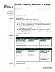
Figure 2. Richard Feynman and other physicists gathered in June 1947 at ShelterIsland, New York, several months before the meeting at the Pocono Manor Inn inwhich Feynman introduced his diagrams. Standing are Willis Lamb (left) and JohnWheeler. Seated, from left to right, are Abraham Pais, Richard Feynman, HermannFeshbach and Julian Schwinger. (Photograph courtesy of the Emilio Segrè VisualArchives, American Institute of Physics.)Figure 3. Electron-electron scattering is described byone of the earliest published Feynman diagrams (featuredin “Sightings,” September–October 2003). Oneelectron (solid line at bottom right) shoots out a forcecarryingparticle—a virtual photon (wavy line)—whichthen smacks into the second electron (solid line at bottomleft). The first electron recoils backward, while thesecond electron gets pushed off its original course. Thediagram thus sketches a quantum-mechanical view ofhow particles with the same charge repel each other. Assuggested by the term “Space-Time Approach” in thetitle of the article that accompanied this diagram, Feynmanoriginally drew diagrams in which the dimensionswere space and time; here the horizontal axis representsspace. Today most physicists draw Feynman diagramsin a more stylized way, highlighting the topology ofpropagation lines and vertices. (This diagram and Figure4 are reproduced from Feynman 1949a, by permissionof the American Physical Society.)interwar architects of QED knew that they couldapproximate this infinitely complicated calculationbecause the charge of the electron (e) is sosmall: e 2 ~1/137, in appropriate units. The chargeof the electrons governed how strong their interactionswould be with the force-carryingphotons: Every time a pair of electrons tradedanother photon back and forth, the equationsdescribing the exchange picked up another factorof this small number, e 2 (see facing page). Soa scenario in which the electrons traded onlyone photon would “weigh in” with the factor e 2 ,whereas electrons trading two photons wouldcarry the much smaller factor e 4 . This event, thatis, would make a contribution to the full calculationthat was less than one one-hundredth thecontribution of the single-photon exchange. Theterm corresponding to an exchange of three photons(with a factor of e 6 ) would be ten thousandtimes smaller than the one-photon-exchangeterm, and so on. Although the full calculationsextended in principle to include an infinite numberof separate contributions, in practice anygiven calculation could be truncated after onlya few terms. This was known as a perturbativecalculation: Theorists could approximate the fullanswer by keeping only those few terms thatmade the largest contribution, since all of theadditional terms were expected to contributenumerically insignificant corrections.Deceptively simple in the abstract, thisscheme was extraordinarily difficult in practice.One of Heisenberg’s graduate studentshad braved an e 4 calculation in the mid-1930s—just tracking the first round of correctionterms and ignoring all others—and quicklyfound himself swimming in hundreds ofdistinct terms. Individual contributions to theoverall calculation stretched over four or fivelines of algebra. It was all too easy to conflateor, worse, to omit terms within the algebraicmorass. Divergence difficulties, acute accountingwoes—by the start of World War II, QEDseemed an unholy mess, as calculationally intractableas it was conceptually muddled.Feynman’s RemedyIn his Pocono Manor Inn talk, Feynman toldhis fellow theorists that his diagrams offerednew promise for helping them march throughthe thickets of QED calculations. As one of hisfirst examples, he considered the problem ofelectron-electron scattering. He drew a simplediagram on the blackboard, similar to the onelater reproduced in his first article on the newdiagrammatic techniques (see Figure 3). Thediagram represented events in two dimensions:space on the horizontal axis and time onthe vertical axis.The diagram, he explained, provided ashorthand for a uniquely associated mathematicaldescription: An electron had a certainlikelihood of moving as a free particle from the158 American Scientist, Volume 93© 2005 Sigma Xi, The Scientific Research Society. Reproductionwith permission only. Contact perms@amsci.org.

point x 1to x 5. Feynman called this likelihoodK +(5,1). The other incoming electron movedfreely—with likelihood K +(6,2)—from pointx 2to x 6. This second electron could then emita virtual photon at x 6, which in turn wouldmove—with likelihood δ +(s 562)—to x 5, wherethe first electron would absorb it. (Here s 56represented the distance in space and time thatthe photon traveled.)The likelihood that an electron would emitor absorb a photon was eγ µ, where e was theelectron’s charge and γ µa vector of Dirac matrices(arrays of numbers to keep track of theelectron’s spin). Having given up some of itsenergy and momentum, the electron on theright would move from x 6to x 4, much the way ahunter recoils after firing a rifle. The electron onthe left, meanwhile, upon absorbing the photonand hence gaining some additional energyand momentum, would scatter from x 5to x 3. InFeynman’s hands, then, this diagram stood infor the mathematical expression (itself writtenin terms of the abbreviations K +and δ +):e 2 ∫∫d 4 x 5d 4 x 6K +(3,5)K +(4,6)γ µδ +(s 562)γ µK +(5,1)K +(6,2)In this simplest process, the two electronstraded just one photon between them; thestraight electron lines intersected with the wavyphoton line in two places, called “vertices.”The associated mathematical term thereforeFeynman diagrams are a powerful tool for making calculationsin quantum theory. As in any quantum-mechanicalcalculation, the currency of interest is a complex number, or“amplitude,” whose absolute square yields a probability. Forexample, A(t, x) might represent the amplitude that a particlewill be found at point x at time t; then the probability of findingthe particle there at that time will be |A(t, x)| 2 .In QED, the amplitudes are composed of a few basicingredients, each of which has an associated mathematicalexpression. To illustrate, I might write:Doing Physics with Feynman Diagramsx1—amplitude for a virtual electron to travel undisturbedfrom x to y: B(x,y);—amplitude for a virtual photon to travel undisturbedfrom x to y: C(x,y); and—amplitude for electron and photon to scatter: eD.Here e is the charge of the electron, which governs howstrongly electrons and photons will interact.Feynman introduced his diagrams to keep track of allof these possibilities. The rules for using the diagrams arefairly straightforward: At every “vertex,” draw two electronlines meeting one photon line. Draw all of the topologicallydistinct ways that electrons and photons can scatter.Then build an equation: Substitute factors of B(x,y) forevery virtual electron line, C(x,y) for every virtual photonline, eD for every vertex and integrate over all of the pointsinvolving virtual particles. Because e is so small (e 2 ~ 1/137,in appropriate units), diagrams that involve fewer verticestend to contribute more to the overall amplitude than complicateddiagrams, which contain many factors of this smallnumber. Physicists can thus approximate an amplitude, A,by writing it as a series of progressively complicated terms.For example, consider how an electron is scattered by anelectromagnetic field. Quantum-mechanically, the field canbe described as a collection of photons. In the simplest case,the electron (green line) will scatter just once from a singlephoton (red line) at just one vertex (the blue circle at point x 0):x 2x 4x 0x1x 3A (1)= eDOnly real particles appear in this diagram, not virtual ones, sothe only contribution to the amplitude comes from the vertex.But many more things can happen to the hapless electron.At the next level of complexity, the incoming electron mightshoot out a virtual photon before scattering from the electromagneticfield, reabsorbing the virtual photon at a later point:x 2A (2)= e 3 ∫D B(1,0) D B(0,2) D C(1,2)In this more complicated diagram, electron lines and photonlines meet in three places, and hence the amplitude forthis contribution is proportional to e 3 .Still more complicated things can happen. At the next levelof complexity, seven distinct Feynman diagrams enter:As an example, we may translate the diagram at upperleft into its associated amplitude:A (3)a= e 5 ∫D B(1,0) D B(0,2) D C(1,3) D× B(3,4) D B(4,3) C(4,2)The total amplitude for an electron to scatter from theelectromagnetic field may then be written:A = A (1)+ A (2)+ A (3)a+ A (3)b+ A (3)c+ ...and the probability for this interaction is |A| 2 .Robert Karplus and Norman Kroll first attempted thistype of calculation using Feynman’s diagrams in 1949;eight years later several other physicists found a series ofalgebraic errors in the calculation, whose correction only affectedthe fifth decimal place of their original answer. Sincethe 1980s, Tom Kinoshita (at Cornell) has gone all the wayto diagrams containing eight vertices—a calculation involving891 distinct Feynman diagrams, accurate to thirteendecimal places!—D.K.www.americanscientist.org 2005 March–April 159© 2005 Sigma Xi, The Scientific Research Society. Reproductionwith permission only. Contact perms@amsci.org.

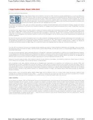
Figure 4. Feynman appended to the article containingFigure 3 a demonstration of how the diagrams serveas “bookkeepers”: this set of diagrams, showing allof the distinct ways that two electrons can trade twophotons back and forth. Each diagram correspondedto a unique integral, all of which had to be evaluatedand added together as part of the calculation for theprobability that two electrons will scatter.Figure 5. Freeman Dyson (right), shown with Victor Weisskopf on a boat en route toCopenhagen in 1952, contributed more than anyone else to putting Feynman diagramsinto circulation. Dyson’s derivation and explanation of the diagrams showed others howto use them, and postdocs trained at the Institute for Advanced Study in Princeton, NewJersey, during his time there spread the use of the diagrams to other institutions. (Photographcourtesy of the Emilio Segrè Visual Archives, American Institute of Physics.)contained two factors of the electron’s charge,e—one for each vertex. When squared, this expressiongave a fairly good estimate for theprobability that two electrons would scatter. Yetboth Feynman and his listeners knew that thiswas only the start of the calculation. In principle,as noted above, the two electrons couldtrade any number of photons back and forth.Feynman thus used his new diagrams todescribe the various possibilities. For example,there were nine different ways that theelectrons could exchange two photons, eachof which would involve four vertices (andhence their associated mathematical expressionswould contain e 4 instead of e 2 ). As in thesimplest case (involving only one photon),Feynman could walk through the mathematicalcontribution from each of these diagrams,plugging in K +’s and δ +’s for each electron andphoton line, and connecting them at the verticeswith factors of eγ µ.The main difference from the single-photoncase was that most of the integrals for the twophotondiagrams blew up to infinity, rather thanproviding a finite answer—just as physicistshad been finding with their non-diagrammaticcalculations for two decades. So Feynman nextshowed how some of the troublesome infinitiescould be removed—the step physicists dubbed“renormalization”—using a combination of calculationaltricks, some of his own design andothers borrowed. The order of operations wasimportant: Feynman started with the diagramsas a mnemonic aid in order to write down therelevant integrals, and only later altered theseintegrals, one at a time, to remove the infinities.By using the diagrams to organize the calculationalproblem, Feynman had thus solveda long-standing puzzle that had stymied theworld’s best theoretical physicists for years.Looking back, we might expect the receptionfrom his colleagues at the Pocono Manor Innto have been appreciative, at the very least. Yetthings did not go well at the meeting. For onething, the odds were stacked against Feynman:His presentation followed a marathon daylonglecture by Harvard’s Wunderkind, JulianSchwinger. Schwinger had arrived at a differentmethod (independent of any diagrams) toremove the infinities from QED calculations,and the audience sat glued to their seats—pausing only briefly for lunch—as Schwingerunveiled his derivation.Coming late in the day, Feynman’s blackboardpresentation was rushed and unfocused.No one seemed able to follow what he wasdoing. He suffered frequent interruptions fromthe likes of Niels Bohr, Paul Dirac and EdwardTeller, each of whom pressed Feynman on howhis new doodles fit in with the established principlesof quantum physics. Others asked moregenerally, in exasperation, what rules governedthe diagrams’ use. By all accounts, Feynmanleft the meeting disappointed, even depressed.Feynman’s frustration with the Pocono presentationhas been noted often. Overlooked inthese accounts, however, is the fact that this confusionlingered long after the diagrams’ inauspiciousintroduction. Even some of Feynman’s160 American Scientist, Volume 93© 2005 Sigma Xi, The Scientific Research Society. Reproductionwith permission only. Contact perms@amsci.org.

closest friends and colleagues had difficulty followingwhere his diagrams came from or howthey were to be used. People such as Hans Bethe,a world expert on QED and Feynman’s seniorcolleague at Cornell, and Ted Welton, Feynman’sformer undergraduate study partner and by thistime also an expert on QED, failed to understandwhat Feynman was doing, repeatedly askinghim to coach them along.Other theorists who had attended the Poconomeeting, including Rochester’s RobertMarshak, remained flummoxed when tryingto apply the new techniques, having to askFeynman to calculate for them since they wereunable to undertake diagrammatic calculationsthemselves. During the winter of 1950,meanwhile, a graduate student and two postdoctoralassociates began trading increasinglydetailed letters, trying to understand why theyeach kept getting different answers when usingthe diagrams for what was supposed tobe the same calculation. As late as 1953—fullyfive years after Feynman had unveiled his newtechnique at the Pocono meeting—Stanford’ssenior theorist, Leonard Schiff, wrote in a letterof recommendation for a recent graduate thathis student did understand the diagrammatictechniques and had used them in his thesis. AsSchiff’s letter makes clear, graduate studentscould not be assumed to understand or be wellpracticed with Feynman’s diagrams. The newtechniques were neither automatic nor obviousfor many physicists; the diagrams did notspread on their own.Dyson and the Apostolic PostdocsThe diagrams did spread, though—thanksoverwhelmingly to the efforts of Feynman’syounger associate Freeman Dyson. Dysonstudied mathematics in Cambridge, England,before traveling to the United States to pursuegraduate studies in theoretical physics. Hearrived at Cornell in the fall of 1947 to studywith Hans Bethe. Over the course of that yearhe also began meeting with Feynman, just atthe time that Feynman was working out hisnew approach to QED. Dyson and Feynmantalked often during the spring of 1948 aboutFeynman’s diagrams and how they could beused—conversations that continued in closequarters when the two drove across the countrytogether that summer, just a few monthsafter Feynman’s Pocono Manor presentation.Later that summer, Dyson attended the summerschool on theoretical physics at the Universityof Michigan, which featured detailedlectures by Julian Schwinger on his own, nondiagrammaticapproach to renormalization. Thesummer school offered Dyson the opportunityto talk informally and at length with Schwingerin much the same way that he had alreadybeen talking with Feynman. Thus by September1948, Dyson, and Dyson alone, had spentintense, concentrated time talking directly withboth Feynman and Schwinger about their newtechniques. At the end of the summer, Dysontook up residence at the Institute for AdvancedStudy in Princeton, New Jersey.Shortly after his arrival in Princeton, Dysonsubmitted an article to the Physical Reviewthat compared Feynman’s and Schwinger’smethods. (He also analyzed the methods ofthe Japanese theorist, Tomonaga Sin-itiro, whohad worked on the problem during and afterthe war; soon after the war, Schwinger arrivedindependently at an approach very similar toTomonaga’s.) More than just compare, Dysondemonstrated the mathematical equivalenceof all three approaches—all this beforeFeynman had written a single article on hisnew diagrams. Dyson’s early article, and alengthy follow-up article submitted that winter,were both published months in advanceof Feynman’s own papers. Even years afterFeynman’s now-famous articles appeared inprint, Dyson’s pair of articles were cited moreoften than Feynman’s.In these early papers, Dyson derived rules forthe diagrams’ use—precisely what Feynman’sfrustrated auditors at the Pocono meeting hadfound lacking. Dyson’s articles offered a “howto” guide, including step-by-step instructionsfor how the diagrams should be drawn andhow they were to be translated into their associatedmathematical expressions. In additionto systematizing Feynman’s diagrams, Dysonderived the form and use of the diagrams fromfirst principles, a topic that Feynman had notbroached at all. Beyond all these clarificationsand derivations, Dyson went on to demonstratehow, diagrams in hand, the troubling infinitieswithin QED could be removed systematicallyfrom any calculation, no matter how complicated.Until that time, Tomonaga, Schwingerand Feynman had worked only with the firstround of perturbative correction terms, andonly in the context of a few specific problems.Figure 6. By the mid-1950s, handy tables like the one including these explanations helpedyoung physicists learn how to translate each piece of their Feynman diagrams into theaccompanying mathematical expression. (Reprinted from Jauch and Rohrlich 1955.)www.americanscientist.org© 2005 Sigma Xi, The Scientific Research Society. Reproductionwith permission only. Contact perms@amsci.org.2005 March–April 161

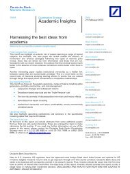
Figure 7. After World War II, the scale of equipment used by high-energy physicistsin the United States grew enormously. Here, E. O. Lawrence and his staff pose withthe newly renovated 184-inch synchrocyclotron at the Berkeley Radiation Laboratory,1946. Such particle accelerators attracted large teams of experimental physicists, whoquickly found themselves keepers of a “zoo” of unanticipated new particles. Studyingthe behavior of these nuclear particles became the order of the day. (Photographcourtesy of Lawrence Berkeley National Laboratory.)Building on the topology of the diagrams, Dysongeneralized from these worked examplesto offer a proof that problems in QED could berenormalized.More important than his published articles,Dyson converted the Institute for AdvancedStudy into a factory for Feynman diagrams. Tounderstand how, we must first step back andconsider changes in physicists’ postdoctoraltraining during this period. Before World WarII, only a small portion of physicists who completedPh.D.’s within the United States went onfor postdoctoral training; it was still commonto take a job with either industry or academiadirectly from one’s Ph.D. In the case of theoreticalphysicists—still a small minority amongphysicists within the U.S. before the war—thoseFigure 8. Faced with the influx of new and unexpected particles and interactions,some theoretical physicists began to use Feynman diagrams as pictures of physicalprocesses. The hope was that simple Feynman diagrams could help the physicistsclassify the new nuclear reactions, even if the physicists could no longer pursue perturbativecalculations. (Reprinted from Marshak 1952.)who did pursue postdoctoral training usuallytraveled to the established European centers.It was only in Cambridge, Copenhagen, Göttingenor Zurich that these young Americantheorists could “learn the music,” in I. I. Rabi’sfamous phrase, and not just “the libretto” of researchin physics. On returning, many of thesesame American physicists—among them EdwinKemble, John Van Vleck, John Slater and J.Robert Oppenheimer, as well as Rabi—endeavoredto build up domestic postdoctoral traininggrounds for young theorists.Soon after the war, one of the key centersfor young theorists to complete postdoctoralwork became the Institute for AdvancedStudy, newly under Oppenheimer’s direction.Having achieved worldwide fame for his roleas director of the wartime laboratory at LosAlamos, Oppenheimer was in constant demandafterward. He left his Berkeley post in1947 to become director of the Princeton institute,in part to have a perch closer to hisnewfound consulting duties in Washington,D.C. He made it a condition of his acceptingthe position that he be allowed to increasethe numbers of young, temporary memberswithin the physics staff—that is, to turn theinstitute into a center for theoretical physicists’postdoctoral training. The institute quicklybecame a common stopping-ground for youngtheorists, who circulated through what Oppenheimercalled his “intellectual hotel” fortwo-year postdoctoral stays.This focused yet informal haven for postdocsproved crucial for spreading Feynmandiagrams around. When Dyson arrived in thefall of 1948—just one year after Oppenheimerbecame director and began to implement hisplan for theorists’ postdoctoral study at theinstitute—he joined a cohort of 11 other juniortheorists. One of the new buildings atthe institute, which was supposed to containoffices for the new visitors, had not been completedon time, so the entire crew of theorypostdocs spent much of that fall semester huddledaround desks in a single office. The closequarters bred immediate collaborations. Veryquickly, Dyson emerged as a kind of ringleader,training his peers in the new diagrammatictechniques and coordinating a series of collaborativecalculations involving the diagrams.One of the most famous of these calculationswas published by two of Dyson’s peers at theinstitute, Robert Karplus and Norman Kroll.After Dyson got them started, they pursuedthe e 4 corrections to an electron’s magnetic moment—thatis, to show how strongly a spinningelectron would be affected by an externalelectromagnetic field. This was a monumentalcalculation involving a long list of complicatedFeynman diagrams. Tracing througheach diagram-and-integral pair as Dyson hadtaught them, the postdocs demonstrated that162 American Scientist, Volume 93© 2005 Sigma Xi, The Scientific Research Society. Reproductionwith permission only. Contact perms@amsci.org.

an electron should have a magnetic momentof 1.001147 instead of 1 (in appropriate units),an answer whose six-place accuracy comparedincredibly well with the latest experimentalmeasurements. Following “much helpful discussionwith F. J. Dyson,” Karplus and Krollthus showed how Feynman diagrams couldbe put to work for calculations no one haddreamed possible before.The Princeton postdocs, personally tutoredin the niceties of diagrammatic calculations byDyson, soon left the institute to take teachingjobs elsewhere. More than four-fifths of all thearticles that used Feynman diagrams in themain American physics journal, the Physical Review,between 1949 and 1954 were submitted bythese postdocs directly, or by graduate students(and other colleagues) whom they trained onarriving at their new jobs. The great majority ofthe 114 authors who made use of the diagramsin the Physical Review during this period did sobecause they had been trained in the new techniquesby Dyson or by one of Dyson’s newlyminted apprentices. (All but two of the remainingauthors interacted directly with Feynman.)The acknowledgments in graduate students’dissertations from geographically disperseddepartments in places including Berkeley, Chicago,Iowa City, Bloomington, Madison, Urbana,Rochester and Ithaca confirm the role of theinstitute postdocs in taking the new techniqueswith them and teaching their own recruits howto use them. In this way, Feynman diagramsspread throughout the U.S. by means of a postdoccascade emanating from the Institute forAdvanced Study.Years later, Schwinger sniffed that Feynmandiagrams had “brought computation to themasses.” The diagrams, he insisted, were a matterat most of “pedagogy, not physics.” Theycertainly were a matter of pedagogy. Lookingat the authors of all these diagrammatic articles,the institute postdocs’ pedagogical missionbecomes clear: More than 80 percent of theauthors were still in the midst of their trainingwhen they began using Feynman diagrams, eitheras graduate students or as postdocs. Mostof the others began using the diagrams whileyoung instructors or assistant professors, lessthan seven years past their doctorates. Olderphysicists simply did not “re-tool.”All the same, the diagrams did not spreadeverywhere. Individuals and even entire departmentsthat remained out of touch with the newlydispersed postdocs failed to make any use of thediagrams, even years after detailed instructionsfor their use had been in print. One of Dyson’sfirst converts at the institute, Fritz Rohrlich (whowent on to publish one of the first textbookson the new diagrammatic techniques), had toadvise a graduate student at the University ofPennsylvania that he should choose a differentdissertation topic or drop out of graduate schoolaltogether; without any representatives from thePrinceton network in town, the student simplywould not be able to get up to speed with thediagrammatic methods.As physicists recognized at the time, muchmore than published research articles orpedagogical texts was required to spread thediagrams around. Personal mentoring andthe postdocs’ peripatetic appointments wereCornellColumbiaChicagoUrbanaOxford/CambridgeFigure 9. As the new diagrams propagated, mentors and students crafted diagrams for different purposes. “Familyresemblances” can be seen in these pairs. In each case the first (left or top) diagram comes from a young instructor,and the second diagram from someone that person trained. Sources: Cornell: Feynman 1949a, Frank 1951; Columbia:Karplus and Kroll 1950, Weneser, Bersohn and Kroll 1953; Rochester: Marshak 1952, Simon 1950; Chicago: Gell-Mann and Low 1951, Wentzel 1953; Urbana: Low 1952, Chew 1954. Oxford and Cambridge: Salam 1951, Ward 1951.Rochesterwww.americanscientist.org© 2005 Sigma Xi, The Scientific Research Society. Reproductionwith permission only. Contact perms@amsci.org.2005 March–April 163

the key. Very similar transfer mechanismsspread the diagrams to young theorists inGreat Britain and Japan, while the hardeningof the Cold War choked off the diagrams’spread to physicists in the Soviet Union. Onlywith the return of face-to-face workshopsbetween American and Soviet physicists inthe mid-1950s, under the “Atoms for Peace”initiatives, did Soviet physicists begin to useFeynman diagrams at anything resemblingthe pace in other countries.The Diagrams DominateSchwinger’s disparaging comments aside, theefficiency of using Feynman diagrams for perturbativecalculations within QED was simplyundeniable. Given the labyrinthine nature ofthe correction terms in these calculations, andthe rapidity and ease with which they could beresolved using the diagrams, one would haveexpected them to be dispersed and used widelyfor this purpose. And yet it didn’t happen.Only a handful of authors published high-orderperturbative calculations akin to Karplus andKroll’s, trotting out the diagrams as bookkeepersfor the ever-tinier wisps of QED perturbations.Fewer than 20 percent of all the diagrammaticarticles in the Physical Review between1949 and 1954 used the diagrams in this way.Instead, physicists most often used the diagramsto study nuclear particles and interactionsrather than the familiar electrodynamicinteractions between electrons and photons.Dozens of new nuclear particles, such as mesons(now known to be composite particlesthat are bound states of the nuclear constituentscalled quarks and their antimatter counterparts),were turning up in the new government-fundedparticle accelerators of postwarAmerica. Charting the behavior of all thesenew particles thus became a topic of immenseexperimental as well as theoretical interest.Yet the diagrams did not have an obviousplace in the new studies. Feynman and Dysonhad honed their diagrammatic techniquesfor the case of weakly interacting electrodynamics,but nuclear particles interact strongly.Whereas theorists could exploit the smallnessof the electron’s charge for their perturbativebookkeeping in QED, various experimentsindicated that the strength of the couplingforce between nuclear particles (g 2 ) was muchlarger, between 7 and 57 rather than 1/137. Iftheorists tried to treat nuclear particle scatteringthe same way they treated photon-electronscattering, with a long series of more and morecomplicated Feynman diagrams, each containingmore and more vertices, then each higherorderdiagram would include extra factors ofthe large number g 2 . Unlike the situation inQED, therefore, these complicated diagrams,with many vertices and hence many factorsof g 2 , would overwhelm the lowest-order contributions.Precisely for this reason, Feynmancautioned Enrico Fermi late in 1951, “Don’tbelieve any calculation in meson theory whichuses a Feynman diagram!”Despite Feynman’s warning, scores of youngtheorists kept busy (and still do!) with diagrammaticcalculations of nuclear forces. In fact, morethan half of all the diagrammatic articles in thePhysical Review between 1949 and 1954 appliedthe diagrams to nuclear topics, including thefour earliest diagram-filled articles publishedafter Dyson’s and Feynman’s own. Rather thandiscard the diagrams in the face of the breakdownof perturbative methods, theorists clungto the diagrams’ bare lines, fashioning new usesand interpretations for them.Some theorists, for example, began to use thediagrams as physical pictures of collision eventsin the new accelerators. Suddenly flooded by a“zoo” of unanticipated nuclear particles streamingforth from the big accelerators, the theoristscould use the diagrams to keep track of whichparticles participated in what types of interactions,a type of bookkeeping more akin to botanicalclassification than to perturbative calculation.Other theorists used the diagrams as a quickway to differentiate between competing physicaleffects: If one diagram featured two nuclearforcevertices (g 2 ) but only one electromagneticforcevertex (e), then that physical process couldbe expected to contribute more strongly thana diagram with two factors of e and only oneg—even if neither diagram could be formallyevaluated. By the early 1960s, a group centeredaround Geoffrey Chew in Berkeley pushed thediagrams even further. They sought to exhumethe diagrams from the theoretical embeddingDyson had worked so hard to establish and usethem as the basis of a new theory of nuclearparticles that would replace the very frameworkfrom which the diagrams had been derived.Throughout the 1950s and 1960s, physicistsstretched the umbilical cord that had linked thediagrams to Dyson’s elegant, rule-bound instructionsfor their use. From the start, physiciststinkered with the diagrams—adding a new typeof line here, dropping an earlier arrow conventionthere, adopting different labeling schemes—to bring out features they now deemed mostrelevant. The visual pastiche did not emergerandomly, however. Local schools emerged asmentors and their students crafted the diagramsto better suit their calculational purposes. Thediagrams drawn by graduate students at Cornellbegan to look more and more like each otherand less like the diagrams drawn by students atColumbia or Rochester or Chicago. Pedagogyshaped the diagrams’ differentiation as much asit drove their circulation.On theorists pressed, further adapting Feynmandiagrams for studies of strongly interactingparticles even though perturbative calculationsproved impossible. One physicist compared164 American Scientist, Volume 93© 2005 Sigma Xi, The Scientific Research Society. Reproductionwith permission only. Contact perms@amsci.org.

this urge to use Feynman diagrams in nuclearphysics, despite the swollen coupling constant,to “the sort of craniometry that was fashionablein the nineteenth century,” which “made aboutas much sense.” A rule-bound scheme for makingperturbative calculations of nuclear forcesemerged only in 1973, when H. David Politzer,David Gross and Frank Wilczek discovered theproperty of “asymptotic freedom” in quantumchromodynamics (QCD), an emerging theoryof the strong nuclear force, a discovery forwhich the trio received the Nobel Prize in 2004.Yet in the quarter-century between Feynman’sintroduction of the diagrams and this breakthrough,with no single theory to guide them,physicists scribbled their Feynman diagramsincessantly—prompting another Nobel laureate,Philip Anderson, to ask recently if heand his colleagues had been “brainwashed byFeynman?” Doodling the diagrams continuedunabated, even as physicists’ theoretical frameworkunderwent a sea change. For generationsof theorists, trained from the start to approachcalculations with this tool of choice, Feynmandiagrams came first.The story of the spread of Feynman diagramsreveals the work required to craft bothresearch tools and the tool users who will putthem to work. The great majority of physicistswho used the diagrams during the decade aftertheir introduction did so only after workingclosely with a member of the diagrammatic network.Postdocs circulated through the Institutefor Advanced Study, participating in intensestudy sessions and collaborative calculationswhile there. Then they took jobs throughoutthe United States (and elsewhere) and began todrill their own students in how to use the diagrams.To an overwhelming degree, physicistswho remained outside this rapidly expandingnetwork did not pick up the diagrams for theirresearch. Personal contact and individual mentoringremained the diagrams’ predominantmeans of circulation even years after explicitinstructions for the diagrams’ use had been inprint. Face-to-face mentoring rather than thecirculation of texts provided the most robustmeans of inculcating the skills required to usethe new diagrams. In fact, the homework assignmentsthat the postdocs assigned to theirstudents often stipulated little more than todraw the appropriate Feynman diagrams fora given problem, not even to translate the diagramsinto mathematical expressions. Thesestudents learned early that calculations wouldnow begin with Feynman diagrams.Meanwhile local traditions emerged. Youngphysicists at Cornell, Columbia, Rochester,Berkeley and elsewhere practiced drawing andinterpreting the diagrams in distinct ways, towarddistinct ends. These diagrammatic appropriationsbore less and less resemblance toDyson’s original packaging for the diagrams.His first-principles derivation and set of oneto-onetranslation rules guided Norman Kroll’sstudents at Columbia, for example, but weredeemed less salient for students at Rochesterand were all but dismissed by Geoffrey Chew’scohort at Berkeley. Mentors made choices aboutwhat to work on and what to train their studentsto do. As with any tool, we can only understandphysicists’ deployment of Feynman diagrams byconsidering their local contexts of use.Thus it remains impossible to separate theresearch practices from the means by whichvarious scientific practitioners were trained.Within a generation, Feynman diagrams becamethe tool that undergirded calculations ineverything from electrodynamics to nuclearand particle physics to solid-state physics andbeyond. This was accomplished through muchpedagogical work, postdoc to postdoc, mentorto disciples. Feynman diagrams do not occur innature; and theoretical physicists are not born,they are made. During the middle decades ofthe 20th century, both were fashioned as part ofthe same pedagogical process.BibliographyChew, G. F. 1954. Renormalization of meson theory witha fixed extended source. Physical Review 94:1748–1754.Dyson, F. J. 1949a. The radiation theories of Tomonaga,Schwinger, and Feynman. Physical Review 75:486–502.Dyson, F. J. 1949b. The S Matrix in quantum electrodynamics.Physical Review 75:1736–1755.Feynman, R. P. 1949a. The theory of positrons. PhysicalReview 76:749–759.Feynman, R. P. 1949b. Space-time approach to quantumelectrodynamics. Physical Review 76:769–789.Feynman, R. P. 1985. QED: The Strange Theory of Light andMatter. Princeton, N.J.: Princeton University Press.Frank, R. M. 1951. The fourth-order contribution to the selfenergyof the electron. Physical Review 83:1189–1193.Gell-Mann, M., and F. E. Low. 1951. Bound states inquantum field theory. Physical Review 84:350–354.Jauch, J., and F. Rohrlich. 1955. The Theory of Photons andElectrons. Cambridge, Mass.: Addison-Wesley.Kaiser, D. In press. Drawing Theories Apart: The Dispersionof Feynman Diagrams in Postwar Physics. Chicago: Universityof Chicago Press.Karplus, R., and N. M. Kroll. 1950. Fourth-order correctionsin quantum electrodynamics and the magneticmoment of the electron. Physical Review 77:536–549.Low, F. E. 1952. Natural line shape. Physical Review 88:53–57.Marshak, R. E. 1952. Meson Physics. New York: McGraw-Hill.Salam, A. 1951. Overlapping divergences and the S-matrix.Physical Review 82:217–227.Schweber, S. S. 1994. QED and the Men Who Made It: Dyson,Feynman, Schwinger, and Tomonaga. Princeton, N.J.:Princeton University Press.Simon, A. 1950. Bremsstrahlung in high energy nucleonnucleoncollisions. Physical Review 79:573–576.Ward, J. C. 1951. Renormalization theory of the interactionsof nucleons, mesons, and photons. PhysicalReview 84:897–901.Wentzel, G. 1953. Three-nucleon interactions in Yukawatheory. Physical Review 89:684–688.Weneser, J., R. Bersohn and N. M. Kroll. 1953. Fourthorderradiative corrections to atomic energy levels.Physical Review 91:1257–1262.For relevant Web links,consult this issue ofAmerican Scientist Online:http://www.americanscientist.org/IssueTOC/issue/701www.americanscientist.org© 2005 Sigma Xi, The Scientific Research Society. Reproductionwith permission only. Contact perms@amsci.org.2005 March–April 165