2 Seismic Wave Propagation and Earth models

2. Seismic Wave Propagation and Earth models
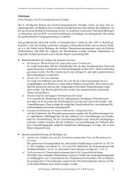
Fig. 2.32 Schematic local travel-time curves (time t over distance x from the source) for a
horizontal two-layer model with constant layer velocities v1 and v2, layer thickness h1 and h2
over a half-space with velocity v3. Other abbreviations stand for: t 1 ic and t 2 ic – intercept times
at x = 0 of the extrapolated travel-time curves for the “head-waves”, which travel with v2
along the intermediate discontinuity between the layers 1 and 2 and with v3 along the
discontinuity between layer 2 and the half-space, respectively. x 1 cr and x 2 cr mark the distances
from the source at which the critically reflected rays from the bottom of the first and the
second layer, respectively, return to the surface. Beyond x 1 co and x 2 co the head-waves from the
bottom of the first and the second layer, respectively, become the first arriving waves (xco -
crossover distance) Rays and their corresponding travel-time curves are shown in the same
color. The full red (violet) travel-time curve relates to the supercritical reflections (i > icr)
from the intermediate (lower) discontinuity while the dotted red (violet) travel-time curve
refers to the respective pre-critical (i < icr) steep angle reflections.
In the case of horizontal layering as in Fig. 2.32 the layer and half-space velocities can be
determined from the gradients dt/dx of the yellow, green and blue travel-time curves which
correspond to the inverse of the respective layer velocities. When determining additionally the
related intercept times t 1 ic and t 2 ic by extrapolating the green and blue curves, or with help of
the crossover distances x 1 co and x 2 co, then one can also determine the layer thickness h1 and h2
from the following relationships:
h1 = 0.5 x 1 co
v1
+ v
v + v
1
2
2
=
0.
5
t
1
ic
v ⋅v
v
1
2
2
2
− v
2
1
and h2
34
t
− 2 h
v
− v
(v ⋅v
)
2
2 2
−1
=
ic
2
1 3 1 1 2
2 2
−1
v 3 − v 2 ⋅(v
2 ⋅v
3 )
. (2.18)
For the calculation of crossover distances for a simple one-layer model as a function of layer
thickness and velocities see Equation (6) in IS 11.1.
In the case where the layer discontinuities are tilted, the observation of travel-times in only
one direction away from the seismic source will allow neither the determination of the proper
sub-layer velocity nor the differences in layer thickness. As can be seen from Fig. 2.33, the
intercept times, the cross-over distances and the apparent horizontal velocities for the
critically refracted head-waves differ when observed down-dip or up-dip from the source
although their total travel times to a given distance from the source remain constant.