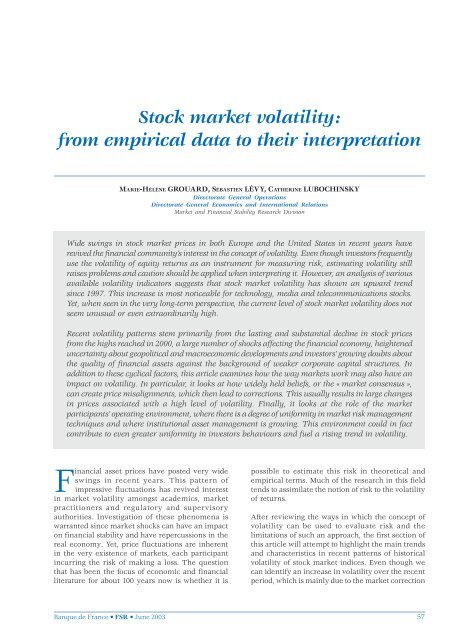
Stock market volatility: from empirical data to their interpretation

Stock market volatility:from empirical data to their interpretationMARIE-HÉLÈNE GROUARD, SÉBASTIEN LÉVY, CATHERINE LUBOCHINSKYDirectorate General OperationsDirectorate General Economics and International RelationsMarket and Financial Stability Research DivisionWide swings in stock market prices in both Europe and the United States in recent years haverevived the financial community’s interest in the concept of volatility. Even though investors frequentlyuse the volatility of equity returns as an instrument for measuring risk, estimating volatility stillraises problems and caution should be applied when interpreting it. However, an analysis of variousavailable volatility indicators suggests that stock market volatility has shown an upward trendsince 1997. This increase is most noticeable for technology, media and telecommunications stocks.Yet, when seen in the very long-term perspective, the current level of stock market volatility does notseem unusual or even extraordinarily high.Recent volatility patterns stem primarily from the lasting and substantial decline in stock pricesfrom the highs reached in 2000, a large number of shocks affecting the financial economy, heighteneduncertainty about geopolitical and macroeconomic developments and investors’ growing doubts aboutthe quality of financial assets against the background of weaker corporate capital structures. Inaddition to these cyclical factors, this article examines how the way markets work may also have animpact on volatility. In particular, it looks at how widely held beliefs, or the « market consensus »,can create price misalignments, which then lead to corrections. This usually results in large changesin prices associated with a high level of volatility. Finally, it looks at the role of the marketparticipants’ operating environment, where there is a degree of uniformity in market risk managementtechniques and where institutional asset management is growing. This environment could in factcontribute to even greater uniformity in investors behaviours and fuel a rising trend in volatility.Financial asset prices have posted very wideswings in recent years. This pattern ofimpressive fluctuations has revived interestin market volatility amongst academics, marketpractitioners and regulatory and supervisoryauthorities. Investigation of these phenomena iswarranted since market shocks can have an impacton financial stability and have repercussions in thereal economy. Yet, price fluctuations are inherentin the very existence of markets, each participantincurring the risk of making a loss. The questionthat has been the focus of economic and financialliterature for about 100 years now is whether it ispossible to estimate this risk in theoretical andempirical terms. Much of the research in this fieldtends to assimilate the notion of risk to the volatilityof returns.After reviewing the ways in which the concept ofvolatility can be used to evaluate risk and thelimitations of such an approach, the first section ofthis article will attempt to highlight the main trendsand characteristics in recent patterns of historicalvolatility of stock market indices. Even though wecan identify an increase in volatility over the recentperiod, which is mainly due to the market correctionBanque de France • FSR • June 2003 57

Stock market volatility: from empirical data to their interpretationunder way since 2000, a longer-term view puts thesevolatility levels into perspective and shows that awider-ranging investigation is necessary. The secondsection of the article analyses this increasedvolatility. It distinguishes between short-termexplanatory factors and structural factors, such asthe impact of innovations in investment products andfund management techniques.1| Uncertainty, risk and volatility:from theory to empirical dataEver since F. Knight’s famous book was published in1921, distinction between risk, which can be measuredin terms of mathematical probabilities, anduncertainty, which cannot be measured, has beenapplied to many fields. In finance, for example,estimated asset price fluctuations are used to evaluatemarket risk and unforeseeable price swings areassumed to reflect uncertainty. Volatility of returnsis the most widely used concept for representing risk.Historical volatility is used to analyse past or presentprices and expected volatility (or the implied volatilityderived from option prices) is used to predict futureprice changes. Under this approach, the only realproblem for the various agents in the financialeconomy stems from unexpected volatility.After a review of the reasons for using volatility asan instrument for evaluating risk, with theunderstanding that it is merely an approximationand that the perception of risk varies for differenttypes of market participants, empirical observationsshow a recent increase in volatility on the main stockmarkets, albeit to different degrees in differentindustries. We also observe more frequent volatilitypeaks in the recent past. In a longer-termperspective, this paper highlights the persistence ofhigh volatility levels.1|1 A review of some conceptsVolatility as a proxy for riskUnder the assumption of a normal distribution ofreturns (i.e. stock prices follow a random walkprocess), which means that the distribution ofreturns is symmetrical, one can estimate theprobabilities of potential gains or losses associatedwith each amount. This means the standarddeviation of securities returns, which is calledhistorical volatility and is usually calculated as amoving average, can be used as a risk indicator. Theprices used for the calculations are usually theclosing prices, but Parkinson (1980) suggests thatthe day’s high and low prices would provide a betterestimate of real volatility. One can also refine theanalysis with high frequency data. Such data enableto avoid the bias stemming from the use of closing(or opening) prices, but they have only been availablefor a relatively short time. The length of theobservation period is another topic that is still underdebate. There are no criteria that enable to concludethat volatility calculated in relation to mean returnsover 20 trading days (or one month) and thenannualised is any more or less representative thanvolatility calculated over 130 trading days (or sixmonths) and then annualised, or even than volatilitymeasured directly over 260 trading days (one year).However, in reality, the distribution of returns isnot normal. This raises a first problem stemmingfrom financial agents’ preferences. Theirpreferences are asymmetrical since they arenaturally much more concerned about the risk oflosses than by the risk of gains. Other riskmeasurements have therefore been developed. Mostof them, including the ones recommended byprudential authorities, focus primarily on the notionof potential loss. More specifically, one can calculatethe semi-variance, which corresponds to a variancecalculated solely on the basis of negative deviationsfrom the mean, the Value at Risk (VaR) or the extremepotential loss for a portfolio at a given time horizonand confidence interval. For example, betweenJanuary 2000 and March 2003, the historical volatilitycalculated for the CAC index, based on the annualisedstandard deviation of daily returns is 20%, whereasthe volatility calculated on the basis of the“semi-standard deviation” is 29.2%.Furthermore, it is restrictive to estimate only thefirst two moments of the distribution of returns(mean and variance), since the distributions can alsobe characterised by their third and fourth moments(skewness and kurtosis). This is a problem as theassumption of a normal distribution is rejected andit is admitted that the distribution of returns isskewed and leptokurtic (see box 1). For example,58 Banque de France • FSR • June 2003

Stock market volatility: from empirical data to their interpretationtake two distributions: one that is normal (A) andone that is not (B). B may be a riskier distribution interms of Value at Risk, because it is more leptokurtic.Yet, it may have a smaller standard deviation thanthat of distribution A, because the probabilities ofreturns in B are more centered around the mean.Yet, all of the risk models based on volatilitymeasured by the standard deviation would show thatB is less risky than A.Box 1Formal presentation of the main conceptsContinuous return: t= LnMean return:SStr[ ]where S: security price or portofolio valuern∑rt = tt= 1nt –1Ln: napierian logarithmwhere n: number of observationsIf r tis normally distributed with a mean µ and a standard deviation σ, then the expected arithmetic return is:2+2µ σE(R t) =eStandard deviation:n∑tσ = t = 1 r( r r )n12Volatility is expressed as percent per year obtained by annualising the standard deviation.Semi-variance:sσrn2 =∑t = 1t( r r )n12for any r t≤ r if we are interested in returns below the mean.Value at Risk: VaR q(X) = the probability q that the loss will exceed an amount X over a given period(1-q that the loss does not exceed X over the given period). With a normal distribution,VaR q= E(r t) + Z q.σ rwhere Z qcorresponds to the quantile associated with probability q.Skewness of the distribution (third moment) s =( ) 3n∑ r t rn t = 13( n 1 )( n 2 ) σrIf the distribution is symmetrical (normal distribution), the skewness coefficient is equal to zero.Kurtosis (thickness of distribution tails, fourth moment) k =( )n 4r r( n∑n + 1)tt = 1( n 1)( n 2)( n 3)σ 4rA normal distribution has a kurtosis coefficient equal to 3. A coefficient greater than 3 indicates thick tails andthe distribution is qualified as leptokurtic.Banque de France • FSR • June 2003 59

Stock market volatility: from empirical data to their interpretationIn illiquid markets, prices may not change over acertain period simply because no transactions takeplace. In this case, low volatility should not beinterpreted as indicating low market risk. It should beseen as a sign of high liquidity risk instead.Furthermore, wide price fluctuations may be necessaryin an illiquid market in order to match bid and offertransactions. In this case, the high price volatility isdue to illiquidity and not to changes in the fundamentalvalue of the assets. In other words, liquidity may be acritical factor for interpreting volatility.Clearly, volatility analysis alone does not providecomplete information about the market risk incurredby financial agents. Volatility is an approximate andbiased indicator of risk, both in the case of empiricalvolatility calculated from past prices (historicalvolatility) and in the case of implied volatility derivedfrom option prices.In any case, volatility has to be estimated since itcannot be observed directly. Several models havebeen constructed to represent the dynamics of thevolatility of returns and to attempt to forecast it. Thesemodels are very frequently autoregressive conditionalheteroskedasticity (ARCH) models, which wereintroduced by Engle in 1982 and then extended byBollersev in 1986 with the Generalised ARCH(GARCH) model. These models introduced explicitmodelling of the variance of returns. This variancefollows a specific temporal process. Thus, given thehistorical information, the conditional distribution ofreturns is normal with a mean equal to zero andvariance of h t, which is a function of historicalvariance. This makes it possible to introduce acorrelation between returns and thereby formallyrepresent persistence phenomena (see Avouyi-Doviet al., 2002). These models, which have limitedpredictive powers, do not fall within the scope of thisarticle. The volatility measurement used here istherefore that of the historical standard deviation.But it is important to keep in mind the limits of thisvolatility indicator as an instrument for measuringthe risk incurred by financial agents.Different perceptions of riskThe diversity of financial agents (ranging fromtheoreticians to practitioners) concerned with theconcept of volatility explains the diversity of theapproaches used to deal with this concept and thedebates surrounding it. All market participants havetheir own perception of risk (risk aversion function).The problem is to reconcile the theoretical conceptsof risk with risk estimates made by the investors whohave adopted the notion of volatility.Following Granger (2002), a typology of agents wouldmake a distinction between:– mathematicians, who are interested in optionpricing theory, using a continuous-time approach.The need to integrate price volatility forecastinto option pricing led to thorough modellingof this forecasting and highlighted severalcharacteristics, such as the decreasing termstructure of volatility. Since volatility is the onlynon-observable component in an option price,reasoning directly in terms of volatility is the sameas reasoning in terms of prices. Thus, “implied”volatility derived from traded option pricescorresponds to the mean volatility expected bymarket participants;– econometricians and empirical statisticians. ARCH,GARCH and other models have revealed thephenomena of heteroskedasticity and volatilitypersistence (see 2|2 below). These approacheshave also highlighted the limitations of thenormally distributed returns assumption and thusthe limitations of historical volatility for assessingmarket risk, as well as the mean reversioncharacteristic of volatility;– economists using uncertainty theory. They workon portfolio theory, on the benefits ofdiversification, through the distinction madebetween specific risk and systematic risk, and onthe Capital Asset Pricing Model (CAPM), in whichvolatility plays a critical role in determiningreturns;– fund managers and traders (“marketprofessionals”), whose objective is basically tomaximise returns on their transactions (albeit witha different time horizon). For them, pricepredictability depends on volatility, or even thevolatility of volatility. Their behaviour issometimes cited as an explanatory factor ofvolatility (see 2|2 below). As for hedge funds, thediversity of their strategies makes it impossibleto reach any conclusions about the impact of theirbehaviour on volatility. Nevertheless, it is widelyagreed that their arbitrage strategies improvesmarket efficiency and that their transactionsimprove market liquidity;60 Banque de France • FSR • June 2003

Stock market volatility: from empirical data to their interpretation– individual investors are typically concerned aboutfalling prices, especially when their retirementpension depends on stock market investments.Individual investors are also more concernedabout the volatility of specific securities than thevolatility of stock market indices. These indicesshow less volatility when there is less correlationbetween securities.This classification should be expanded to includeprudential authorities and central banks, which areconcerned about the potential impact of increasedvolatility on systemic risk and financial stability.1|2 Empirical observations:volatility has showna rising trend since 1997A global phenomenonA widespread increase in volatilityThere has been a sharp increase in stock marketvolatility in all western countries in the recent past.This followed a period in the first half of thenineteen-nineties, when volatility levels were verylow. The movement began in the second half of thenineteen-nineties, as shown in the chart 1, whichplots the annual historical volatility of some majorstock market indices. After large increases between1997 and 1999, volatility stabilised at a high levelbefore resuming its upward trend in 2001. Annualhistorical volatility reached levels in excess of 15 to20 percentage points above the mean estimated over15 years. In 2002 and 2003, the annual historicalvolatility of the CAC index was greater than 38%,whereas monthly volatility occasionally hit 60%(see charts 1 and 2).Comparing volatility patterns in variousindustrialised countries reveals their similarity. Allof the main stock market indices, whose correlationhas increased over the last ten years, have shownfairly similar volatility patterns. Japan is the onlycountry in this group where the volatility pattern isdifferent from that in the industrialised countries.Equity returns in Japan are less correlated with thosein US and European markets, primarily becauseJapan’s business cycle is not correlated with thoseof the United States or Europe.Chart 1Annual historical volatility of the SP 500,CAC 40 and FTSE 100 stock market indices(in %)4035302520151051988 1990 1992 1994 1996 1998 2000 2002CAC 40FTSE 100SP 500Sources: Banque de France, BloombergImplied volatility analysis confirms the rising trendin stock market volatility. In the French market,implied volatility derived from CAC 40 option pricesreached 60% on occasion in 2002 and 2003. Ananalysis of the differential between implied volatilityand historical volatility seems to confirm an increasein investors’ uncertainty over the last six years.Implied volatility was several percentage pointshigher than historical volatility (an average of2.5 percentage points between 1997 and 2003 in thecase of the CAC 40). This widening of the differentialindicates that investors expect volatility to increasein the future. On the other hand, when historicalvolatility increases sharply, the differential betweenimplied and historical volatility usually turnsnegative, thus signalling that volatility is expectedto return to more moderate levels. It is noteworthythat the decline in monthly historical volatilitybetween September 2002 and March 2003 was notaccompanied by a fall in implied volatility, whichremained high, testifying to investors’ persistentuncertainties.Banque de France • FSR • June 2003 61

Stock market volatility: from empirical data to their interpretationChart 2Monthly implied and historical volatilityof the CAC 40 index(in %)655545352515211470- 7- 14Differences between industries can explain someof the differences in the volatility levels betweenthe indices, as can be seen in charts 3 and 4. Inthe recent past, the proportion of technology,telecommunications and media stocks in each indexseems to largely account for the mean volatilitydifferences between indices.Chart 3Index average monthly historical volatility (1987-2002)(in %)Nikkei5- 21S1 S2 S1 S2 S1 S2 S12000 2001 2002 2003Monthly realised volatilityImplied volatilityDifferential (implied – realised) (right-hand scale)NasdaqCAC 40EuroStoxx 50Sources: Banque de France, BloombergDifferences in volatility levelsbetween indices and industriesEven though volatility patterns look similar for allindices, substantial differences between the volatilitylevels of indices can be seen. The monthly historicalvolatility of the CAC 40 index stands at 20%, whereasthat of the EuroStoxx and SP 500 indices stands atjust under 16%. Such differences arise from combinedfactors linked to the indices composition. The mainstock market indices usually include the largest marketcapitalisations on the national stock exchange, buttheir composition varies greatly. The number ofcompanies included, the volatility of the individualstocks tracked and the degree of diversification, asshown by the covariances between the stocks tracked,can differ significantly.Similarly, the volatility of stock prices in differentindustries can also vary substantially. The data froma broad European index (EuroStoxx) show that someindustries like construction, food processing andutility, have registered very little volatility comparedto other industries. Their stock prices have been lessvolatile than the index itself. On the other hand,technology stocks, telecommunications stocks and,to a lesser extent, media stocks posted historicalvolatility over the same period that was more than10 percentage points greater than the volatility ofthe index (see chart 4).EuroStoxxDow JonesSP 500FTSE 100Sources: Banque de France, Bloomberg12 14 16 18 20 22Chart 4Monthly historical volatility for each industryin the EuroStoxx index since 1990(in %)TechnologyTelecomMediaAutomobileCyclical goodsInsuranceHealthEnergy (oil)ChemicalsNon cyclical goodsRetailBasic resourcesBankingFinanceIndustryOverall indexUtilityAgri-foodConstruction14 16 18Sources: Banque de France, Bloomberg20 22 24 26 283062 Banque de France • FSR • June 2003

Stock market volatility: from empirical data to their interpretationChart 5Annualised 6-month historical volatilityof the SP 500 and Nasdaq indices(in %)60504030201001973 1978 1983 1988 1993 1998 2003SP 500NasdaqSources: Banque de France, BloombergChart 6Monthly historical volatility and proportionof TMT stocks in broad indices(Proportion of TMT stocks / Monthly realised volatility)5550Nasdaq4540353025EuroStoxx20FTSE15 All-ShareBE 500Topix10 FTSE350SPSBF 250SP 50051 50016 18 20 22 24 26 28 30 32Sources: Banque de France, BloombergVolatility peaks have been more frequentand lasted longer since 1997Estimating volatility peaksIn addition to an increase in average volatility, therecent past has also seen an increase in the frequencyof volatility peaks, as illustrated by short-term volatilitypatterns in the charts 1, 2 and 5. A volatility peak is aphase during which volatility reaches a much higherlevel than its long-term mean. It can be determinedempirically by analysing the distribution of volatility.Thus, after estimating volatility thresholds on thebasis of the distribution of the monthly historicalvolatility of the SP 500 index over the last 50 years, alook at the recent period allows two comments:– a sharp increase in the number of volatility peaksregardless of the thresholds chosen over 95% 1 . Thus,between 1997 and 2003, 6 out of the 7 yearsshowed volatility peaks at high distributionthresholds (up to 98%). This is the first time thatsuch a configuration has appeared in 50 years.Before that, volatility peaks were short-lived andspaced out;– an increase in the duration of volatility peaks, so muchso that some peaks could be called “volatilityplateaus”. Historical volatility reached the 97%threshold in 2002 and stayed there for 73 days.The only time it was greater was in 1950.Chart 7Number of days on which the monthly volatilityof the SP 500 index stood at an exceptional level2002200120001998199719891988198719821974197319701962195519500 20 40 60 80 100 12098% threshold (volatility level of 31.0%)97% threshold (volatility level of 27.7%)Sources: Banque de France, BloombergIntraday volatilityObservation of intraday volatility, measured by thepercent change between the highest and lowest pricesreached during a trading day, confirms the precedingremarks. The intraday volatility pattern of theFTSE index shows an increase in the number andduration of volatility peaks very clearly (see chart 8). Italso highlights another distinctive feature of volatility1A “95% threshold” means that 95% of the observations in the sample are lower than the level selected. In the case of the SP 500, the 95%,97%, 98% and 99% thresholds correspond to volatility levels over 20 days of 24.3%, 27.7%, 31.0% and 34.7% respectively.Banque de France • FSR • June 2003 63

Stock market volatility: from empirical data to their interpretationduring this period. Even though volatility peaks aremore frequent and last longer, they are not as high.The intraday volatility observed in the recent past hasnever exceeded the levels seen during the stock marketcrash of 1987, when variations of 14% in a single daywere seen. Since 1997, with the exception of 10%variations within a day seen during the Asian crisis,the largest variations between daily highs and lowsrange from 4% to 8%. In the current period, the salientfact is not the level of volatility during peaks, but thelength of time over which volatility remains high.Chart 8Intraday variation in the FTSE index moving averageand 6-month historical volatility(in %)– a slightly different volatility indicator, thesix-month average of absolute daily variations,reveals that the recent past appears exceptionalcompared to earlier episodes. The volatility levelmeasured in this way in 2002 and 2003 was thehighest observed in the United States in the last75 years. It stood at more than 25%, which isslightly higher than the levels seen in 1987 and1929. This seems to confirm that the currentperiod is exceptional, not because of the extremevariations in stock prices, but because thevariations are large and long lasting.Chart 9Annualised historical volatility of the SP 500 index3.5143.02.52.01.51.00.50.001986 1988 1990 1992 1994 1996 1998 2000 20026-month moving average (left-hand scale)6-month historical volatility (left-hand scale)Intraday variation (right-hand scale)NB: Data are not annualised.Sources: Banque de France, Bloomberg1210864260504030201001932 1942 1952 1962 1972 1982 1992 2002Over six monthsOver five yearsSources: Banque de France, BloombergIs current stock market volatilityexceptional from a long term perspective?If we look at a longer period of time, which is onlypossible for the United States, where available datastretch back to the beginning of the twentiethcentury, it seems difficult to conclude that historicalvolatility has reached an unusual level. Volatilitylevels in the recent past differ depending on theindicators used to measure them:– a six-month volatility indicator shows that therecent peak of volatility (31%) has only beenobserved four times in the last 75 years: after thecrash of 1929, during World War 2, during the1973 oil shock and during the 1987 stock marketcrash. At these times, and more particularly inthe nineteen-thirties, volatility reached muchhigher levels (60% in 1930 and 45% in 1987);Chart 10Annualised moving average of daily absolute variationsof the SP 500 index3025201510501932 1942 1952 1962 1972 1982 1992 2002Six-month moving averageFive-year moving averageSources: Banque de France, Bloomberg64 Banque de France • FSR • June 2003

Stock market volatility: from empirical data to their interpretationThese two indicators offer different views of the samephenomenon. Using the standard deviation to calculatevolatility tracks the average deviation of returns fromthe mean return for the period. If the daily variation instock prices were 1% during the period, volatility wouldbe equal to zero. Calculating volatility from the meanabsolute returns is more in line with the intuitive“impression of volatility” produced through observationof market trends. Under this approach, if the dailyvariation in prices stands at 1% over the whole period,volatility would be equal to 1%.Using both measurements over substantiallylonger periods of five years confirms the previousobservation and highlights another longer-termtrend. After declining between the nineteen thirtiesand the mid nineteen-sixties, volatility started to riseagain and the trend has continued since then, exceptfor one short interruption at the beginning of thenineteen-nineties.2| Interpreting the recent volatility patternDo the rising trend of volatility and the more frequentvolatility peaks stem from cyclical phenomena linked tothe characteristics of the current period, with a sharpdecline in stock prices, doubts about the criteria used forasset pricing and high levels of corporate debt? Or arethey the result of structural factors, linked to the waycapital markets operate, investors’ asset managementtechniques or even to financial instruments themselves?Even though there seems to be an undeniablelink between current volatility and currentcircumstances, we should still investigate whetherthe development of certain management techniqueshas had an impact on capital markets.2|1 Analysis of the macro-financialenvironment has becomemore difficultMore frequent shocks and growing uncertaintyIn an analytical framework where the price offinancial assets is determined by discountingexpected future dividends, prices change when newinformation arrives. Important news leads to majorvariations in prices and, ultimately, to an increasein volatility. The recent increase in volatility stemsfrom a conjunction of phenomena that are specificto the recent past. These include:– more frequent major shocks. The Asian crisis in1997, the Russian crisis and its impact onemerging economies in 1998 (Brazil), the crisisof the LTCM hedge fund in the same year, theevents of 11 September 2001, and the Argentinecrisis in 2001 were all exceptional shocks thatradically changed investors’ perception of risk andthe outlook for growth;– a general increase in uncertainty about macroeconomicoutlook. This phenomenon has been particularlymarked since the business cycle upturn in 2000,owing to the distinctive characteristics of the latestrecovery, which started as a rapid V-shaped recovery,then slowed to a U-shaped recovery, and even aW-shaped recovery. Under these circumstances, thegeopolitical uncertainty that has prevailed in thewake of the 11 September attacks and the UnitedStates’ action in Afghanistan and Iraq has had aneven greater impact on stock market price swings;– greater volatility of corporate earnings. In keepingwith the traditional approach to asset pricing, stockprice volatility and volatility of corporate earningsappear to be empirically linked 2 (Shiller, 2000).The price volatility of stocks in the SP 500 indexat the end of the nineteen-nineties matched thevolatility of earnings per share, as the chart belowshows.Chart 1112-month historical volatility of SP 500 stock priceand earnings per share(in %)22.520.017.515.012.510.07.55.001970 1974 1978 1982 1986 1990 1994 1998 2002SP 500 (left-hand scale)Earnings per share (right-hand scale)Sources: Banque de France, Schiller14121086422However, Shiller shows that dividend volatility is not the only explanation for price volatility.Banque de France • FSR • June 2003 65

Stock market volatility: from empirical data to their interpretationEarnings volatility and, simultaneously, the volatilityof projected earnings, were more intimately linkedto stock price volatility after 2000, when analystsfaced growing difficulties in assessing earningsprojections. Reflecting frequent and substantialrevisions of earnings expectations, the analysts’ ownforecasts became more volatile (see chart 12). Theanalysts’ revision of earnings forecasts started in 2000and increased substantially in 2001. This change isnoteworthy, since the revised forecasts focused onrecurring income, i.e. profits from firms’ corebusiness, and excludes non-recurring items, suchas write-offs of goodwill.“New economy” stock prices dropped and prospectswere highly revised as investors and analysts’earnings projections were trimmed to morereasonable levels as start up companies’ profits werepostponed.Chart 12Analysts’ revisions of earnings forecastsfor CAC 40 companies(in %)20- 2- 4- 6- 8- 10- 12- 141996 1997 1998 1999 2000 2001 2002Two months earlier Six months earlierNB: Revisions of forecasts made two or six months earlier.Source: JCFThe financial information required to valueassets is not reliable enoughEver since the stock market bubble burst in 2000, achain of events caused market participants toquestion their quality assessments of financialassets. This increase in the risk associated withholding such assets contributed to an increase in thevolatility of securities. The deterioration of assetquality stems from three phenomena:– doubts about the accuracy of corporate financialstatements in the wake of various scandals, suchas the Enron and Worldcom affairs, whichrevealed accounting fraud in the United Statesand the collusion of the auditors responsible forvetting the statements. This had an especiallybig impact on investors, since corporate financialstatements are the key to asset valuation.Financial scandals involving leading companiesled to fears of widespread fraud, whichsubstantially increased the perceived riskincurred by owning securities issued by theprivate sector and ultimately increased volatility;– doubts about the robustness of information providedby rating agencies, as these agencies downgradedmany companies’ ratings very suddenly in therecent past. This makes the signals given byratings particularly weak. What good is theprotection offered by owning “investment grade”securities if, in the next six months, they can bedowngraded to “speculative grade” or even “default”?– doubts about the advice of financial analysts withregard to the prices or potential changes in equities,following scandals in which it was revealed thatfinancial institutions gave their customersrecommendations that were contrary to their realassessments of issuing firms. This type of scandal,which shook investors’ confidence in stock values,had an even greater impact on their risk perceptionsbecause the improper recommendations weregiven by leading international investment banks.These three major elements, which increased therisk associated with owning securities issued by theprivate sector, therefore led to increased volatility.In times of high risk, any minor news may bringabout a radical change in the investors’ valuations.A very weak firm can suddenly be transformed froma company on the brink of bankruptcy into a viableone and vice-versa, which can lead to big swings instock prices. On the other hand, a company withsound fundamentals would be subject to smallershifts in investors’ perceptions and, therefore, itsshare price would be less volatile.Economic and statistical propertiesof volatilityFalling stock prices and rising volatilityThe increase in volatility seen since 2000 has takenplace against the backdrop of falling stock prices.This confirms that, while some volatility is a featureof rising stock prices, market corrections usuallylead to much greater volatility. This asymmetricalvolatility response can be seen in the chart 13, which66 Banque de France • FSR • June 2003

Stock market volatility: from empirical data to their interpretationcompares the average monthly variation of theCAC 40 index with its historical monthly volatility.For the same variation in prices over one month,volatility tends to be higher if the variation isnegative. For example, a price increase of 8 to 10%leads to average volatility of 18%, whereas drop inprices of the same magnitude leads to averagevolatility of more than 30%.Chart 13Volatility and the CAC 40 index (1987-2003):volatility skewAverage volatility level and mean variations of the index(in %)454035302520151050≤ -10- 8 - 6 - 4 - 2 0 2 4 6 8 10 ≥the productive sector at the macroeconomic level.In recent decades, this ratio has usually movedin parallel to volatility. When corporate debt rises,volatility increases, as has been the case since1997. On the other hand, the marked declinein corporate debt between the end of thenineteen-eighties and the mid-nineteen-ninetiescorresponds to a decrease in volatility in theUnited States.There were two reasons for the increase incorporate debt in the second half of thenineteen-nineties. First, firms were underfinancial pressure to produce higher returnson equity (ROE targets of 15% became standard)and they could increase earnings per shareby increasing leverage; secondly, industrialstrategies led firms to make major investmentsin order to gain positions in innovativesectors such as technology, media andtelecommunications;Chart 14Stock market volatility and debt ratiosof non-financial firms in the United States(Percent – Annual data)Sources: Banque de France, Bloomberg2270This volatility skew 3 may seem surprising. If weconsider, in keeping with conventional asset pricingtheory, that news moves asset prices, there is noapparent reason for “bad” news that depresses stockprices to produce more overall volatility than “good”news. In practice, there are two phenomena thatseem to explain this skewed response:– leverage — as measured by the ratio of total debtto equity —, which moves in the opposite directionto stock prices. Good news raises prices andreduces leverage, thus alleviating the associatedrisk and thereby reducing volatility. Merton’sresearch showed that the more highly leverageda firm is, the more volatile its shares are.Empirically speaking, it seems that the increasein leverage when stock markets decline leads toweakening of corporate capital structures. Thismeans that in the event of a downturn in thebusiness cycle or bad news, a highly-leveragedfirm automatically becomes riskier and its shareprice more volatile.Changes in the ratio of non-financial firms’ debtto GDP can be used to track the indebtedness of3Engle and Ng (1993), Zakoian (1994),Wu and Xiao (1999).4Pindyck (1984), French, Schwert and Stambaugh (1987).2018161412108351964 1968 1972 1976 1980 1984 1988 1992 1996 2000Five-year historical volatility of the SP 500(left-hand scale)Debt ratios of non-financial firms in the United States(right-hand scale)Sources: Banque de France, Bloomberg– the feedback effect or the intertemporal variationin the risk premium, which does not depend onthe impact of price variations, like the financialleverage effect does, but on expected volatility 4 .For example, expectations of an increase involatility, in an uncertain international context,depress domestic stock prices, investors askingfor a higher return in exchange for incurring ahigher risk. Thus, when market risks increase,volatility rises. This hypothesis is based on thefact that present and expected volatility bothincrease during periods when there is lots ofnews.656055504540Banque de France • FSR • June 2003 67

Stock market volatility: from empirical data to their interpretationThis effect can explain the volatility skew for themarket as a whole, as represented by an index, andfor individual stocks, since the covariance between astock returns and the market returns is positive. Wu(2001) shows that the feedback effect is more powerfulwhen the covariance between individual stock returnsand market return is higher, which is the case for badnews (higher than in the case of good news).These two effects put forward to explain the volatilityskew involve two different types of causality. Theleverage hypothesis is based on the idea that variationin prices causes change in volatility, whereas theintertemporal variation in the risk premium hypothesisassumes that the change in prices results from achange in expected volatility. These two factors cansimultaneously affect prices, as stressed by Wu (2001).The feedback effect, which depresses stock priceswhen expected volatility increases, causes leverageto increase. This then in turn increases risk andvolatility. However, according to Campbell andHentschel (1992), market trends can reverse, whichmeans that the feedback effect is the weaker of thetwo effects.Volatility persistence and mean reversionThe persistence of high volatility levels is one of thestatistical characteristics of volatility. Volatility occursin clusters, as a quick look at the charts in section 1|2shows. In other words, major swings in asset pricesdo not suddenly stop after major news breaks. Instead,they tend to persist. This volatility persistence meansthat market participants’ volatility expectations areinfluenced by their perception of high volatility (Poterbaand Summers, 1986).The other noteworthy statistical property of volatilityis its tendency to revert to the mean. Mean reversionmeans that, even though shocks lead to largevariations in prices and an increase in volatility, theireffects eventually wear off.These properties raise several problems whenanalysing the current situation, since the timerequired for volatility to revert to the mean is unknown.Analysis of the various phases of volatility clusteringsdoes not reveal any truly comparable mean reversionperiods. Moreover, the mean depends on theinherently arbitrary choice of observation period.This then raises the question of the “normal” volatilitylevel. This is a particularly difficult question to answer,since markets, along with the macroeconomicenvironment, are constantly changing, which makeshistorical comparisons a delicate matter.2|2 Does the way capital marketsoperate fuel price volatility?Conventions, herd behaviour and divergencebetween stock prices and fundamentalsThe valuation of financial assets, by discountingexpected future cash flows, is particularly difficultin the case of shares, where the future cash flowsare based on earnings forecasts for the next year,the expected rate of earnings growth and thediscount rate. Under the assumption of an efficientmarket (informational efficiency), even though allthe information needed to estimate theseparameters is available, the real problem lies ininterpreting the information. A degree of subjectivityexplains why different agents may have differentinterpretations of the information and the opinionsof others have to be taken into account in theinformation. Therefore, the analytical frameworkis both conventional and “consensual” (Aglietta inCercle des Économistes – 2002) and within it, capitalasset prices may deviate from their fundamentalvalue.This gives rise to an explanatory model of marketprices, based on a “market consensus” which isfuelled by all market participants, includinganalysts, strategists and investors. The participantsare deemed to behave rationally in this model. Theirinvestment decisions are based on the mostcomprehensive assessment that they can make ofthe value of available assets at a given time. Thisdetermines the equilibrium prices, which integrateall available information and thus reflect the“conventional” fundamental value of the underlyingassets.The market conventions concern the general analysisof the macroeconomic environment, the judgmentabout the prospects for various industries and anymicro and macroeconomic and financial indicatorsdeemed to be relevant and their interpretation.Behavioural finance has revealed a number ofcognitive and behavioural “biases”, particularly whenit comes to processing information. These “biases”were obvious during the “new economy” bubble,more specifically in the case of Internet andtelecommunications stocks. Since they could not useconventional indicators to justify the prices of thesestocks, market participants relied on new ad hocvaluation measures based on such shaky criteria asthe number of subscribers, instead of actual orexpected earnings. Furthermore, some analysts68 Banque de France • FSR • June 2003

Stock market volatility: from empirical data to their interpretationfocused too narrowly on certain financial ratios, suchas EBITDA 5 , and some companies abused pro formapresentations of their financial statements, which ledto the same type of biased reasoning. A great deal ofresearch has shown that the format used to presentfinancial data gives rise to biases in the perception ofrisks and has an impact on investment decisions 6 .As long as nobody challenges the market consensus,the pricing framework is likely to create self-fulfillingprice dynamics. Market participants are bound tooverweight short-term trends and extrapolate them,rather than engage in fundamental long-term analysis.Any change in market prices in the “expected” directionwill quickly be seen as confirming the soundness ofthe originally held beliefs and will make these beliefsstronger. On the other hand, as soon as a newexplanatory model challenges this consensus, marketprices will adjust to the new fundamental values,which are just as conventional as the earlier values.The longer the former model held sway and the morewidely accepted it was, the larger the price adjustmentswill be 7 .The shift from one market convention to another isoften the result of greater uncertainty about economicfactors, such as economic growth, and financialfactors, such as liquidity. In the meantime herdbehaviour takes hold and is rationalised byinformation and reputation considerations like therelative performances of fund managers. Suchbehaviour is associated with periods of greatervolatility, since it leads to an increase in the numberof transactions and, more importantly, to “same way”pressures which can create liquidity problems.It took some time to refute the “new economy”market consensus. Rather than revising theirlong-term growth projections overnight, marketparticipants seem to have become gradually awareof the excesses of the previous period and adjustedtheir positions as they went along, as reflected inthe overall high level of volatility and the steepdecline in stock prices. The major revisions affectedtechnology, telecommunications and media stocks,since the previous valuation criteria were particularlyshaky and arbitrary. It also led to substantial revisionsof earnings growth forecasts with long-lasting highvolatility levels.Market participants’ operating environmentand market dynamicsMarket participants operate within a restrictiveframework that potentially influences asset pricingdynamics. The main aspects of this issue stem frommarket risk management and from institutional assetmanagement.Market risk managementValue at Risk (VaR) and Daily Earnings at Risk (DEaR)are widely used risk management concepts. Allfinancial institutions use them, as do fund managersoperating under liquidity constraints. These systemsare used to estimate the risk of loss incurred on aportfolio (a set of positions) at a given time horizon,depending on past volatility and the correlationsbetween the assets contained in the portfolio.Logically enough, they show that the less correlationthere is between assets in a portfolio (i.e. the morediversified the portfolio), the smaller the risk of netlosses is. While we do not question the usefulnessof these risk measurement methods, the way inwhich they are being used is a cause for concern.– The measures proposed by these systems areusually associated with loss limits. When theselimits are reached, “contingency” measures aretriggered: portfolios are reallocated by selling offthe most volatile assets or the most highlycorrelated assets in favour of less risky and morediversified assets, margin calls and/or demandsfor extra collateral are imposed on marketparticipants by the credit institutions providingtheir funding. When an initial shock, such as dropin stock prices combined with a sudden increasein volatility, means that such measures areimplemented by large numbers of marketparticipants simultaneously, they can amplifymarket movements, add to the volatility of theassets that were the most volatile to begin withand cause a spillover of destabilising price5EBITDA: Earnings Before Interest, Taxes, Depreciation and Amortisation. This financial ratio is similar to the gross operating surplus(excédent brut d’exploitation (EBE)) used in France.6Siebenmorgen, Weber and Weber (2000)7The prevailing market consensus during the market bubble seen at the end of the previous decade was, roughly speaking, that growth wasexpected to be strong and the equity risk premium was expected to be low. The degree to which investors adhered to this consensus can be seenin surveys. For example, Shiller’s surveys of individual investors show that 95% of those surveyed in 1999 and in 2000 thought that “The stockmarket is the best investment for long-term investors, who are able to buy securities and hold them throughout market ups and downs.”Moreover, 91% and 80% of those surveyed in 1999 and 2000 respectively agreed with the statement “If a market crash like that of 1987should happen, the market is bound to climb back up to its previous levels in a few years.”Banque de France • FSR • June 2003 69

Stock market volatility: from empirical data to their interpretationBox 2CMF report on increased stock market volatility (December 2002)In an attempt to identify the factors behind the stock market volatility observed since 2001, the French CapitalMarket Council (Conseil des marchés financiers) published an interim report in December 2002 that sets out anumber of hypothesis and topics for discussion and investigation in conjunction with market professionals. Thesearch for possible sources of volatility can take different directions.– Issuers: weaker corporate capital structures. In addition to the direct effects of excessive debt (leverage),the report looks into the potentially amplifying effect of some of the borrowing procedures that were widelyused in recent years. It focuses more particularly on hybrid instruments, such as convertible bonds, and theuse of contingency clauses, such as rating triggers. The report also looks into the possible role played byshare buybacks and the procedures for granting and managing stock options.– Investors: institutional asset management procedures. The report mentions various institutional fundmanagement techniques, including benchmarking and “alternative” management. The report lays morespecific emphasis on the role played by management strategies that rely on leverage and the practice of shortselling.– Intermediaries: The increasing trade in credit risk and interactions between credit markets and equitymarkets, on the one hand, and the growth of option markets, on the other hand, mean that the report putsforward a third topic for discussion on the market dynamics associated with credit risk managementand option position management.The report is an interim report offered as a first step in discussions that need to be taken further. It shows just howcomplex any analysis of the causes of volatility will be. It even acknowledges that “it would be premature to comeup with all-encompassing, clear-cut and definitive conclusions” at this stage.dynamics. At the same time, these dynamics maystrengthen the initial correlations between variousassets, which is likely to provide further fuel forthe movements described above. This leads tooverreaction in asset price movements.– Volatility peaks on capital markets are usuallyassociated with lower market liquidity. An illiquidmarket is bound to have more problems inproviding counterparties for a big surge inone-way orders. The risk managementmechanisms discussed here may cause liquidityto dry up, if they result in a large number of marketparticipants switching from one market to anothersimultaneously. The combination of excessivelyuniform behaviour (see below) and riskmanagement systems that give users similarsignals at the same time is likely to fuelself-sustaining dynamics.The same types of dynamics may occur whenaccounting or prudential rules require marketparticipants to mark to market their portfolios andpositions, regardless of the investment strategyguiding such positions or the liquidity of theunderlying markets 8 .Institutional asset management structuresThe institutional asset management industry hasgrown rapidly over the last twenty years and theimpact of this growth on the pricing dynamics incapital markets has been the subject of intense debateamongst academics and practitioners alike. At firstsight, one could think that these institutionalinvestors, such as mutual funds or pension fundsand their managers, would be less sensitive thanothers to the pressures created by the short-termmarket movements described above because they8See Matherat (S.) (2003): “International accounting standardisation and financial stability”, Banque de France, Financial Stability Review,June70 Banque de France • FSR • June 2003

Stock market volatility: from empirical data to their interpretationare experienced market professionals who useadvanced asset allocation techniques and take amedium-to-long-term approach for their investmentstrategies.Yet, it could be feared that some of the features ofthe industry structure actually add to marketimbalances and thereby increase price volatility.– Most institutional management is based onbenchmarking. This means that managers arejudged on their relative performance with regardto a market benchmark, which is usually a stockindex, rather than on their performance inabsolute terms.– Managers’ performances are usually measuredand compared to that of their peers over fairlyshort periods of a quarter to a year, even thoughthe investment strategies they use ought to beassessed over the medium term.– Furthermore, their income is directly linked tothe amount of assets under management and notto their actual performance.These factors combine to increase fundmanagers’ sensitivity to short-term marketmovements and promote uniform investmentbehaviour, with limited deviations from benchmarkindices or even replication of these indices. Thesefactors can even lead to herd-like behaviour amongstfund managers. Dennis and Strickland (2002) havedemonstrated that, during periods of turmoil onAmerican stock markets, the stocks showing thegreatest downwards variations during market declinesand the greatest upwards variations during marketrises were the most actively traded ones and thosefor which mutual funds and pension funds were thelargest shareholders: this simply derives from thefact that it has an impact on market liquidity.This pattern may be reinforced by the fact that UCITSand mutual funds operate under severe liquidityconstraints. They must be able to honour finalinvestors’ demands to cash out at any time on thebasis of the market value of their portfolio. Thiscreates an added incentive for such funds to shadowtheir benchmark as closely as possible, particularlyin times of market turbulence.Financial techniques and instruments:ambiguous links to volatilityThe question of whether some financial techniquesor instruments may be an endogenous source ofvolatility in financial asset prices has come up before.The answers are neither clear-cut nor definitive.Proliferation of contingency procedures and clausesThere are recurring suspicions that financialinnovation and the growing complexity of thetechniques and instruments used by marketparticipants actually contribute to stock marketvolatility. It is particularly the case for option typeproducts. One common feature of many of thefinancial instruments developed in recent years isthat they implicitly or explicitly incorporate options.This is the case of convertible bonds, investmentproducts offering capital or performance guaranteesand bonds with contingency clauses.With the growth of options markets, volatility or, tobe more precise, expected volatility has become acommodity that market professionals now trade andmanage like any other commodity. This makes itpossible to transfer volatility risk between marketparticipants. Volatility can also be sought out andexplicit positions can be taken that are disconnectedfrom the other risks on the underlying asset.Yet, it is difficult to see how options could be a sourceof additional volatility. What is being transferred withthe volatility risk is a summarised and direct form ofthe risk of a variation in the price of a financial assetor a stock market index 9 . The changes in impliedvolatility reveal to the market as a whole the changesin expected volatility, meaning the perception of therisk associated with an underlying asset.Market techniques: short sellingShort selling enables a participant who does notactually own securities to borrow them, and thensell them on the spot market. The objective is to buythe securities back later, hopefully at a lower price,and pay back the initial loan. The opposite of shortselling is buying securities on credit. Short selling isoften suspected of amplifying price movements onthe spot market and increasing market volatility by9Volatility swaps and volatility futures make it possible to take direct positions on the implied volatility contained in certain stock market indices.Banque de France • FSR • June 2003 71

Stock market volatility: from empirical data to their interpretation“artificially” increasing downwards pressure onprices, since the shorted securities are not sold bytheir actual owners, which tend to be institutionalinvestors as a general rule. However, it is difficult todraw any conclusions on this point because of thelack of transparency surrounding the use of thistechnique. Any judgment on this matter needs totake the following observations into consideration.– When market makers engage in short selling(securities loans to market participants are oneof the instruments commonly used in marketmaking and a necessary instrument for thisactivity), they improve market liquidity and shouldthus help to reduce volatility. On the other hand,when short selling is part of a purely speculativestrategy, it should be analysed as taking a positionon the expected future value of a security. Thedifference between the selling and buying pricesmust be greater than the cost of the loan to justifythe transaction. The analysis of such speculativetransactions belongs to the more generaldiscussion on whether speculation has a stabilisingor destabilising impact.– Questions about short selling are similar to thequestions raised about the use of futures contractswith regard to spot market transactions, sincefutures are easier to use because of their lowtransaction costs and because of the leverage theyoffer. These characteristics make futures marketsleading markets that transmit signals to spotmarkets. These same characteristics mayexplain why short selling may have a great,albeit temporary, impact on spot markets,particularly in shallow and illiquid markets. As ageneral rule, the depressive effect of short sellingon stock prices ought to be offset quite rapidly,since the borrowed securities need to be returnedto their owner. Yet, the “net” effect of suchtransactions is not necessarily neutral.Bandwagon effects or herd-like behaviour mayappear when a lack of transparency means thatmarket participants are unable to discern thenature of such transactions and the resulting pricemovements may themselves be triggering factorsfor specific dynamics. For example, suchmovements could affect the issuer’s bonds as aresult of rating triggers based on stock marketprices.It would probably be an oversimplification to attribute most of the observed increase in asset pricevolatility to the techniques and instruments used by market participants. Even though theseinstruments may accentuate volatility, by amplifying market trends, it is primarily because theyenable market participants to express their expectations more efficiently, more rapidly and at a lowercost. With real-time trading, the constant pressure of new information and the growing interdependencyof markets, under certain circumstances, the complexity and diversity of market instruments promoteexcessive risk-taking and erratic behaviour by giving participants the illusion that they will be ableto sell off any position easily. But the primary causes of volatility lie in the marketparticipants’ behaviour and in the interactions between their behaviour and the techniques availableto them. Therefore, the development of increasingly complex and technically efficient markets in amacro-financial environment that does not always have the same degree of efficiency andresponsiveness (owing to excessively uniform behaviour, the market consensus, rules-based investmentstrategies and the constraints imposed by regulations, operating rules or accounting rules) couldcontribute to a rise in average stock market volatility at levels, in certain periods, higher than thatobserved today.72 Banque de France • FSR • June 2003

Stock market volatility: from empirical data to their interpretationBibliographyAglietta (M.) (2002): « Efficience et rationalité dans lesmarchés boursiers : les raisons du scepticisme », le cercledes Économistes, « Les marchés sont-ils rationnels ? »Anderson (T.), Bollersev (T.), Diebold (F.) andEbens (H.) (2000): “The Distribution of Stock ReturnVolatility”, National Bureau of Economic Research ,Working Paper n° 7933 , OctoberArtus (P.) (2003): “Volatilité des prix d’actifs et politiquemonétaire”, Colloque international de la Banque deFrance, Paris, 7 MarchAvouyi-Dovi (S.), Guégan (S.) et Ladoucette (S.)(2002): « Une mesure de la persistance dans lesindices boursiers », Banque de France Working Papern° 94, DecemberBlack (F.) (1976): “Studies of Stock Price VolatilityChanges”, Proceedings of the 1976 Meetings of theAmerican Statistical Association, Business andEconomical Statistics Section, p. 177-181Buchalet (J.-L.) (2002): “Maintien à un haut niveau dela volatilité des estimations de bénéfice des indices”, JCFOutlook, JCF Group, 17 MayCampbell (J.), Hentschel (L.) (1992): “No News isGood News: An Asymmetric Model of ChangingVolatility in Stock Returns”, Journal of FinancialEconomics, n° 31, p. 281-318Campbell (J.) and Lettau (M.) (1999): “Dispersionand Volatility in Stock Returns: an EmpiricalInvestigation”, National Bureau of EconomicResearch, Working Paper n°7144 , MayCampbell (J.), Lettau (M.), Malkiel (B.) and Xu (Y.)(2001): “ Have Individual Stocks Become MoreVolatile? An empirical Exploration of IdiosyncraticRisk”, The Journal of Finance, volume LVI, n°1,February, p. 1-43Chauveau et al. (2003): “La volatilité des marchésaugmente-t-elle ? Théorie et mise en perspectivehistorique”, Discussion Paper n°1, Network for Researchin Finance, MarchChristie (A. A.) (1982): “The Stochastic Behavior ofCommon Stock Variances – Value, Leverage andInterest Rate Effects”, Journal of FinancialEconomics 10, p. 407-432Conseil des marchés financiers (2002): Rapport d’étapesur l’augmentation de la volatilité du marché des actions,DecemberDanielsson (J.) (2002): “The Emperor has no Clothes:Limits to Risk Modelling”, Journal of Banking andFinance n°26, p. 1273-1296Dennis (P. J.) and Strickland (D.) (2002): “Who blinksin Volatile Markets, Individuals or Institutions?”,Journal of Finance, OctoberEngle (R. F.) and Ng (V. K.) (1993): “Measuring andTesting the Impact of News on Volatility”, Journal ofFinance 48, p. 1749-1778French (K. R.), Schwert (G. W.) and Stambaugh (R.)(1987): “Expected Stock Returns and Volatility”,Journal of Financial Economics 19, p. 3-29Garman (M.) and Klass (M.) (1980): “On theEstimation of Securities Price Volatilities fromHistorical Data”, The Journal of Business, volume 53,issue 1, January, p. 67-78Granger (C.) (2002): “Some Comments on Risk”,Journal of Applied Econometrics n°17, p.447-456Jondeau (E.) (2001): “Volatilité et mésalignement surles marchés financiers”, Bulletin de la Banque de Francen°95, November, p. 67-76Jorion (P.) (2002): “Fallacies about the Effects ofMarket Risk Management Systems”, FinancialStability Review, Bank of England, December,p. 115-127Knight (F.) (1921): « Risk Uncertainty and Profit »Reprint Chicago, The Chicago University Press 1971Parkinson (M.) (1980): “The Extreme Value Methodfor Estimating the Variance of the Rate of Return”,Journal of Business, volume 53, n° 1, p. 61-65Pindyck (R. S.) (1984): “Risk, Inflation, and the StockMarket”, American Economic Review 74, p. 334-351Banque de France • FSR • June 2003 73

Stock market volatility: from empirical data to their interpretationPoterba (J.) and Summers (L.) (1984,1986): “ThePersistence of Volatility and Stock MarketFluctuations”, National Bureau of EconomicResearch, Working Paper n°1462, September, AmericaEconomic Review 76, p. 1142-1151Shiller (R. J.) (2000): “Irrational Exuberance”,Princeton University PressSchwert (G.) (1989), “Why does Stock MarketVolatility Change over Time?”, Journal of Finance,volume XLIV, n°5, December, p. 1115-1151Wu (G.) (2001): “The Determinants of AsymmetricVolatility”, Review of Financial Studies, n° 14,p. 837-859Wu (G.) et Xiao (Z.) (1999), “A Generalized PartiallyLinear Model of Asymmetric Volatility”, WorkingPaper, University of MichiganZakoian (J. M.) (1994), “Threshold HeteroskedasticModels”, Journal of Economic Dynamics andControl 18, p. 931-955Schwert (G.) (1998), “Stock Market Volatility : TenYears After the Crash”, National Bureau of EconomicResearch , Working Paper n°6381, JanuarySiebenmorgen (N.), Weber (E.) et Weber (M.) (2000),“Communicating Asset Risk: How the Format ofHistorical Volatility Information Affects RisksPerception and Investment Decisions”, SFB504,University of Mannheim, August74 Banque de France • FSR • June 2003