Projective transformation of pseudo-Riemannian manifolds

Vladimir MatveevJena (Germany)Geodesic equivalence of Einsteinpseudo-Riemannian metrics andprojective Lichnerowicz conjectureKiosak–M∼: arXiv:0806.3169 and arXiv:0810.0994slides posted on www.minet.uni-jena.de/∼matveev/

How Isaac Newton found the gravitational law?.

How Isaac Newton found the gravitational law?Isaac Newton in Philosophiae Naturalis Principia Mathematicasuggested the following strategy to study nature:.

How Isaac Newton found the gravitational law?Isaac Newton in Philosophiae Naturalis Principia Mathematicasuggested the following strategy to study nature:.

How Isaac Newton found the gravitational law?Isaac Newton in Philosophiae Naturalis Principia Mathematicasuggested the following strategy to study nature:◮ one needs to understand the mathematical modeldescribing the situation, and then.

How Isaac Newton found the gravitational law?Isaac Newton in Philosophiae Naturalis Principia Mathematicasuggested the following strategy to study nature:◮ one needs to understand the mathematical modeldescribing the situation, and then◮ find the parameters in the model usingexperiments or observations..

How Isaac Newton found the gravitational law?Isaac Newton in Philosophiae Naturalis Principia Mathematicasuggested the following strategy to study nature:Example:Gravitational Law:◮ one needs to understand the mathematical modeldescribing the situation, and then◮ find the parameters in the model usingexperiments or observations.r.

How Isaac Newton found the gravitational law?Isaac Newton in Philosophiae Naturalis Principia Mathematicasuggested the following strategy to study nature:Example:Gravitational Law:r◮ one needs to understand the mathematical modeldescribing the situation, and then◮ find the parameters in the model usingexperiments or observations.From the Newton’s third law and general sense itis clear that the gravitational force between twobodies is proportional to the masses of the bodiesand depends on the distance between the bodies:F = F 1 = F 2 = m 1 m 2 · f (r)..

How Isaac Newton found the gravitational law?Isaac Newton in Philosophiae Naturalis Principia Mathematicasuggested the following strategy to study nature:Example:Gravitational Law:r◮ one needs to understand the mathematical modeldescribing the situation, and then◮ find the parameters in the model usingexperiments or observations.From the Newton’s third law and general sense itis clear that the gravitational force between twobodies is proportional to the masses of the bodiesand depends on the distance between the bodies:F = F 1 = F 2 = m 1 m 2 · f (r). How to find f ?.

How Isaac Newton found the gravitational law?Isaac Newton in Philosophiae Naturalis Principia Mathematicasuggested the following strategy to study nature:Example:Gravitational Law:r◮ one needs to understand the mathematical modeldescribing the situation, and then◮ find the parameters in the model usingexperiments or observations.From the Newton’s third law and general sense itis clear that the gravitational force between twobodies is proportional to the masses of the bodiesand depends on the distance between the bodies:F = F 1 = F 2 = m 1 m 2 · f (r). How to find f ?Newton tried different functions for f and solved the equationsof motion. He proved that for the function f (r) = G r 2the trajectories of the planets are ellipses which was observedby Kepler..

How Isaac Newton found the gravitational law?Isaac Newton in Philosophiae Naturalis Principia Mathematicasuggested the following strategy to study nature:Example:Gravitational Law:r◮ one needs to understand the mathematical modeldescribing the situation, and then◮ find the parameters in the model usingexperiments or observations.From the Newton’s third law and general sense itis clear that the gravitational force between twobodies is proportional to the masses of the bodiesand depends on the distance between the bodies:F = F 1 = F 2 = m 1 m 2 · f (r). How to find f ?Newton tried different functions for f and solved the equationsof motion. He proved that for the function f (r) = G r 2the trajectories of the planets are ellipses which was observedby Kepler..

How Isaac Newton found the gravitational law?Isaac Newton in Philosophiae Naturalis Principia Mathematicasuggested the following strategy to study nature:Example:Gravitational Law:r◮ one needs to understand the mathematical modeldescribing the situation, and then◮ find the parameters in the model usingexperiments or observations.From the Newton’s third law and general sense itis clear that the gravitational force between twobodies is proportional to the masses of the bodiesand depends on the distance between the bodies:F = F 1 = F 2 = m 1 m 2 · f (r). How to find f ?Newton tried different functions for f and solved the equationsof motion. He proved that for the function f (r) = G r 2the trajectories of the planets are ellipses which was observedby Kepler..

How Isaac Newton found the gravitational law?Isaac Newton in Philosophiae Naturalis Principia Mathematicasuggested the following strategy to study nature:Example:Gravitational Law:r◮ one needs to understand the mathematical modeldescribing the situation, and then◮ find the parameters in the model usingexperiments or observations.From the Newton’s third law and general sense itis clear that the gravitational force between twobodies is proportional to the masses of the bodiesand depends on the distance between the bodies:F = F 1 = F 2 = m 1 m 2 · f (r). How to find f ?Newton tried different functions for f and solved the equationsof motion. He proved that for the function f (r) = G r 2the trajectories of the planets are ellipses which was observedby Kepler. Then, he concluded that the functionf (r) is indeed G r, i.e., F = F 2 1 = F 2 = G m1m2r. 2

Let us apply the same method to the general relativity

Let us apply the same method to the general relativityThe model is known since Einstein: the structure of thevacuum space-time is given by a solution of the Einsteinequations R ij = R n g ij.

Let us apply the same method to the general relativityThe model is known since Einstein: the structure of thevacuum space-time is given by a solution of the Einsteinequations R ij = R n g ij.In many cases, the only objects one can observe are geodesicsconsidered as unparameterized curves

Let us apply the same method to the general relativityThe model is known since Einstein: the structure of thevacuum space-time is given by a solution of the Einsteinequations R ij = R n g ij.In many cases, the only objects one can observe are geodesicsconsidered as unparameterized curves (since thereis no notion of absolute time).The clock ofobject hasnothing to dowith the clockof the observerThe clock ofobserver hasnothing to dowith the clockof the object

In many cases, the only thing one can obtain byobservations are unparametrized geodesics

In many cases, the only thing one can obtain byobservations are unparametrized geodesics

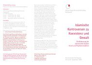
In many cases, the only thing one can obtain byobservations are unparametrized geodesicsOne can obtainunparametrized geodesics by observation:Observer N 1InformationInformationObserver N 2We take 4 freely falling observersthatmeasure the angular coordinate of the visible objectsand send this information to one place. This place will have4 functions angle(t) for every visible objectwhich are in general case 4 coordiantes of the object.

In many cases, the only thing one can get by observationsare unparametrised geodesics

In many cases, the only thing one can get by observationsare unparametrised geodesicsIf one can not register a periodic process on the observedbody, one can not get the own time of the bodyThis situation is extremelyrare

As it is known since Weyl and Ehlers, if one knows the light cone(i.e., the conformal structure), one can reconstruct the own time ofan free falling object.

As it is known since Weyl and Ehlers, if one knows the light cone(i.e., the conformal structure), one can reconstruct the own time ofan free falling object.

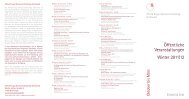
As it is known since Weyl and Ehlers, if one knows the light cone(i.e., the conformal structure), one can reconstruct the own time ofan free falling object.The only way to get the light cone is to send the light ray to the objectand to register echo -- also possible very rarelyand register echoechoworld line ofthe observerthe light ray to the bodyobserver shootswith light in objects

Question to answer

Question to answer(H. Weyl 1931): Could two 4-dimensional Einstein metrics ofLorenz signature have the same geodesics considered as unparameterizedcurves?

Question to answer(H. Weyl 1931): Could two 4-dimensional Einstein metrics ofLorenz signature have the same geodesics considered as unparameterizedcurves?Jürgen Ehlers 1972 We reject clocks as basic tools for settingup the space-time geometry and propose ... freely falling particlesinstead. We wish to show how the full space-time geometrycan be synthesized ... . Not only the measurement of length butalso that of time then appears as a derived operation.

Main Definition and example of Lagrange 1789

Main Definition and example of Lagrange 1789Def. Two metrics (on one manifold) are geodesically equivalent ifthey have the same unparameterized geodesics

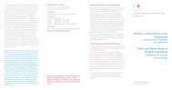
00 1100 110000000000011111111111000000000001111111111100000000000111111111110000000000000000000000000000000000000000000011111111111111111111111111111111111111111111010101010000000000000000000000000000000001111111111101011111111111101011111111111101000000000001111111111101000000000001111111111100000000000111111111110000000000011111111111000000000001111111111100000000000111111111110000000000011111111111000000000001111111111101000000000000000000000000000000000111111111111111111111111111111111010100000000000111111111110101010100 1100 1100 11Main Definition and example of Lagrange 1789Def. Two metrics (on one manifold) are geodesically equivalent ifthey have the same unparameterized geodesics (notation: g ∼ ḡ)f(X)X0Radial projection f : S 2 → R 2 takesgeodesics of the sphere to geodesicsof the plane,

00 1100 110000000000011111111111000000000001111111111100000000000111111111110000000000000000000000000000000000000000000011111111111111111111111111111111111111111111010101010000000000000000000000000000000001111111111101011111111111101011111111111101000000000001111111111101000000000001111111111100000000000111111111110000000000011111111111000000000001111111111100000000000111111111110000000000011111111111000000000001111111111101000000000000000000000000000000000111111111111111111111111111111111010100000000000111111111110101010100 1100 1100 11Main Definition and example of Lagrange 1789Def. Two metrics (on one manifold) are geodesically equivalent ifthey have the same unparameterized geodesics (notation: g ∼ ḡ)f(X)X0Radial projection f : S 2 → R 2 takesgeodesics of the sphere to geodesicsof the plane, because geodesicson sphere/plane are intersectionof plains containing 0 with thesphere/plane.

Examples of Dini 1869

Examples of Dini 1869Theorem (Dini 1869) The metric(X(x) − Y (y))(dx 2 + dy 2 ) (is geodesically equivalent tothey have sense).1Y(y) − 1X(x)) (dx 2X(x) + dy2Y(y)), (if

Examples of Dini 1869Theorem (Dini 1869) The metric(X(x) − Y (y))(dx 2 + dy 2 ) (is geodesically equivalent tothey have sense).1Y(y) − 1X(x)) (dx 2X(x) + dy2Y(y)), (ifMoreover, every two nonproportional Riemannian geodesically equivalentmetrics on the surface have this form in a neighbourhood of almost everypoint.

Examples of Dini 1869Theorem (Dini 1869) The metric(X(x) − Y (y))(dx 2 + dy 2 ) (is geodesically equivalent tothey have sense).1Y(y) − 1X(x)) (dx 2X(x) + dy2Y(y)), (ifMoreover, every two nonproportional Riemannian geodesically equivalentmetrics on the surface have this form in a neighbourhood of almost everypoint.Levi-Civita 1896:The metrics of Dini can be generalized forevery dimension.

Examples of Dini 1869Theorem (Dini 1869) The metric(X(x) − Y (y))(dx 2 + dy 2 ) (is geodesically equivalent tothey have sense).1Y(y) − 1X(x)) (dx 2X(x) + dy2Y(y)), (ifMoreover, every two nonproportional Riemannian geodesically equivalentmetrics on the surface have this form in a neighbourhood of almost everypoint.Levi-Civita 1896:The metrics of Dini can be generalized forevery dimension.In the pseudo-Riemannian case there existother examples

Examples of Dini 1869Theorem (Dini 1869) The metric(X(x) − Y (y))(dx 2 + dy 2 ) (is geodesically equivalent tothey have sense).1Y(y) − 1X(x)) (dx 2X(x) + dy2Y(y)), (ifMoreover, every two nonproportional Riemannian geodesically equivalentmetrics on the surface have this form in a neighbourhood of almost everypoint.Levi-Civita 1896:The metrics of Dini can be generalized forevery dimension.In the pseudo-Riemannian case there existother examples (the complete description indim 2 is due to Bolsinov, Pucacco, M∼ 2008;for other dimensions is joint project with Bolsinov)

Main Theorem 1

Main Theorem 1Theorem 1 (Kiosak, M∼ 2009):

Main Theorem 1Theorem 1 (Kiosak, M∼ 2009): 4−dim Einstein manifoldsare geodesically rigid:

Main Theorem 1Theorem 1 (Kiosak, M∼ 2009): 4−dim Einstein manifoldsare geodesically rigid: Let (M 4 ,g) be a pseudo-Riemannian Einsteinmanifold of nonconstant curvature. Then, every ḡ geodesicallyequivalent to g has the same Levi-Civita connection with g.

Main Theorem 1Theorem 1 (Kiosak, M∼ 2009): 4−dim Einstein manifoldsare geodesically rigid: Let (M 4 ,g) be a pseudo-Riemannian Einsteinmanifold of nonconstant curvature. Then, every ḡ geodesicallyequivalent to g has the same Levi-Civita connection with g.It was a popular subject; partial cases of Theorem 1 were proved byWeyl 1921, Couty 1961, Petrov 1963, Ehlers 1972–1977, Mikes 1982,Barnes 1993, Hall (-Lonie) 1995–2007, Kiosak 2000,Mikes-Kiosak-Hinterleitner 2006.

Main Theorem 1Theorem 1 (Kiosak, M∼ 2009): 4−dim Einstein manifoldsare geodesically rigid: Let (M 4 ,g) be a pseudo-Riemannian Einsteinmanifold of nonconstant curvature. Then, every ḡ geodesicallyequivalent to g has the same Levi-Civita connection with g.It was a popular subject; partial cases of Theorem 1 were proved byWeyl 1921, Couty 1961, Petrov 1963, Ehlers 1972–1977, Mikes 1982,Barnes 1993, Hall (-Lonie) 1995–2007, Kiosak 2000,Mikes-Kiosak-Hinterleitner 2006.Remark 1. If there exists an open subset U ⊂ TM

Main Theorem 1Theorem 1 (Kiosak, M∼ 2009): 4−dim Einstein manifoldsare geodesically rigid: Let (M 4 ,g) be a pseudo-Riemannian Einsteinmanifold of nonconstant curvature. Then, every ḡ geodesicallyequivalent to g has the same Levi-Civita connection with g.It was a popular subject; partial cases of Theorem 1 were proved byWeyl 1921, Couty 1961, Petrov 1963, Ehlers 1972–1977, Mikes 1982,Barnes 1993, Hall (-Lonie) 1995–2007, Kiosak 2000,Mikes-Kiosak-Hinterleitner 2006.Remark 1. If there exists an open subset U ⊂ TM• such that it is sufficient big: for every x ∈ M we have T x M ∩ U ≠ ∅(for example, the set of all time-like vectors is sufficiently big),

Main Theorem 1Theorem 1 (Kiosak, M∼ 2009): 4−dim Einstein manifoldsare geodesically rigid: Let (M 4 ,g) be a pseudo-Riemannian Einsteinmanifold of nonconstant curvature. Then, every ḡ geodesicallyequivalent to g has the same Levi-Civita connection with g.It was a popular subject; partial cases of Theorem 1 were proved byWeyl 1921, Couty 1961, Petrov 1963, Ehlers 1972–1977, Mikes 1982,Barnes 1993, Hall (-Lonie) 1995–2007, Kiosak 2000,Mikes-Kiosak-Hinterleitner 2006.Remark 1. If there exists an open subset U ⊂ TM• such that it is sufficient big: for every x ∈ M we have T x M ∩ U ≠ ∅(for example, the set of all time-like vectors is sufficiently big),•• such that every g-geodesic γ with ˙γ(t 0 ) ∈ U is a reparametrizedḡ-geodesic,

Main Theorem 1Theorem 1 (Kiosak, M∼ 2009): 4−dim Einstein manifoldsare geodesically rigid: Let (M 4 ,g) be a pseudo-Riemannian Einsteinmanifold of nonconstant curvature. Then, every ḡ geodesicallyequivalent to g has the same Levi-Civita connection with g.It was a popular subject; partial cases of Theorem 1 were proved byWeyl 1921, Couty 1961, Petrov 1963, Ehlers 1972–1977, Mikes 1982,Barnes 1993, Hall (-Lonie) 1995–2007, Kiosak 2000,Mikes-Kiosak-Hinterleitner 2006.Remark 1. If there exists an open subset U ⊂ TM• such that it is sufficient big: for every x ∈ M we have T x M ∩ U ≠ ∅(for example, the set of all time-like vectors is sufficiently big),•• such that every g-geodesic γ with ˙γ(t 0 ) ∈ U is a reparametrizedḡ-geodesic,Then the metrics g and ḡ are geodesically equivalent.

Main Theorem 1Theorem 1 (Kiosak, M∼ 2009): 4−dim Einstein manifoldsare geodesically rigid: Let (M 4 ,g) be a pseudo-Riemannian Einsteinmanifold of nonconstant curvature. Then, every ḡ geodesicallyequivalent to g has the same Levi-Civita connection with g.It was a popular subject; partial cases of Theorem 1 were proved byWeyl 1921, Couty 1961, Petrov 1963, Ehlers 1972–1977, Mikes 1982,Barnes 1993, Hall (-Lonie) 1995–2007, Kiosak 2000,Mikes-Kiosak-Hinterleitner 2006.Remark 1. If there exists an open subset U ⊂ TM• such that it is sufficient big: for every x ∈ M we have T x M ∩ U ≠ ∅(for example, the set of all time-like vectors is sufficiently big),•• such that every g-geodesic γ with ˙γ(t 0 ) ∈ U is a reparametrizedḡ-geodesic,Then the metrics g and ḡ are geodesically equivalent.Remark 2. Actually, we can prove more: if a metric is close in theC 6 -topology to a Einstein 4-dimensional metric of nonconstant curvature,then it admits no nontrivial geodesic equivalence

Main Theorem 2

Main Theorem 2Theorem 1 is very nontrivial and fails in dimension ≥ 5: there existcounterexamples.

Main Theorem 2Theorem 1 is very nontrivial and fails in dimension ≥ 5: there existcounterexamples. Thought the metrics in the counterexamples are notcomplete:

Main Theorem 2Theorem 1 is very nontrivial and fails in dimension ≥ 5: there existcounterexamples. Thought the metrics in the counterexamples are notcomplete:Theorem 2 (Kiosak, M∼ 2009:) n−dim complete Einsteinmanifolds are geodesically rigid:

Main Theorem 2Theorem 1 is very nontrivial and fails in dimension ≥ 5: there existcounterexamples. Thought the metrics in the counterexamples are notcomplete:Theorem 2 (Kiosak, M∼ 2009:) n−dim complete Einsteinmanifolds are geodesically rigid:Let (M n ,g) be a complete pseudo-Riemannian Einstein manifold ofnonconstant curvature. Then, every complete ḡ geodesically equivalentto g has the same Levi-Civita connection with g.

Proof of main Theorems: reformulaition as PDE

Proof of main Theorems: reformulaition as PDEFolklor (Levi-Civita 1896): Two symmetric affine connections Γ and ¯Γhave the same (unparameterized) geodesics, iff there exists a 1-form φsuch that¯Γ i jk = Γi jk + φ jδk i + φ kδji (∗)

Proof of main Theorems: reformulaition as PDEFolklor (Levi-Civita 1896): Two symmetric affine connections Γ and ¯Γhave the same (unparameterized) geodesics, iff there exists a 1-form φsuch that¯Γ i jk = Γi jk + φ jδ i k + φ kδ i j (∗)Then, all metrics geodesically equivalent to a connection Γ are solutionsof the system

Proof of main Theorems: reformulaition as PDEFolklor (Levi-Civita 1896): Two symmetric affine connections Γ and ¯Γhave the same (unparameterized) geodesics, iff there exists a 1-form φsuch that¯Γ i jk = Γi jk + φ jδk i + φ kδji (∗)Then, all metrics geodesically equivalent to a connection Γ are solutionsof [ the system ]∂∂k ḡij − ḡ ia Γ a kj − ḡ jaΓ a ki− φ i ḡ kj − φ j ḡ ki − 2φ k ḡ ij = 0

Proof of main Theorems: reformulaition as PDEFolklor (Levi-Civita 1896): Two symmetric affine connections Γ and ¯Γhave the same (unparameterized) geodesics, iff there exists a 1-form φsuch that¯Γ i jk = Γi jk + φ jδk i + φ kδji (∗)Then, all metrics geodesically equivalent to a connection Γ are solutionsof [ the system ]∂∂k ḡij − ḡ ia Γ a kj − ḡ jaΓ a ki− φ i ḡ kj − φ j ḡ ki − 2φ k ḡ ij = 0on unknowns ḡ ij and φ i . The system is nonlinear

Proof of main Theorems: reformulaition as PDEFolklor (Levi-Civita 1896): Two symmetric affine connections Γ and ¯Γhave the same (unparameterized) geodesics, iff there exists a 1-form φsuch that¯Γ i jk = Γi jk + φ jδk i + φ kδji (∗)Then, all metrics geodesically equivalent to a connection Γ are solutionsof [ the system ]∂∂k ḡij − ḡ ia Γ a kj − ḡ jaΓ a ki− φ i ḡ kj − φ j ḡ ki − 2φ k ḡ ij = 0on unknowns ḡ ij and φ i . The system is nonlinear andcontains an artificial unknown φ i

Proof of main Theorems: reformulaition as PDEFolklor (Levi-Civita 1896): Two symmetric affine connections Γ and ¯Γhave the same (unparameterized) geodesics, iff there exists a 1-form φsuch that¯Γ i jk = Γi jk + φ jδk i + φ kδji (∗)Then, all metrics geodesically equivalent to a connection Γ are solutionsof [ the system ]∂∂k ḡij − ḡ ia Γ a kj − ḡ jaΓ a ki− φ i ḡ kj − φ j ḡ ki − 2φ k ḡ ij = 0on unknowns ḡ ij and φ i . The system is nonlinear andcontains an artificial unknown φ iRemark. One can actually find the artificial unknown φ in the terms ofg and ḡ:

Proof of main Theorems: reformulaition as PDEFolklor (Levi-Civita 1896): Two symmetric affine connections Γ and ¯Γhave the same (unparameterized) geodesics, iff there exists a 1-form φsuch that¯Γ i jk = Γi jk + φ jδk i + φ kδji (∗)Then, all metrics geodesically equivalent to a connection Γ are solutionsof [ the system ]∂∂k ḡij − ḡ ia Γ a kj − ḡ jaΓ a ki− φ i ḡ kj − φ j ḡ ki − 2φ k ḡ ij = 0on unknowns ḡ ij and φ i . The system is nonlinear andcontains an artificial unknown φ iRemark. One can actually find the artificial unknown φ in the terms ofg and ḡ: indeed, contracting (∗) with respect to i and j, we obtain¯Γ a ai = Γ a ai + (n + 1)φ i.

Proof of main Theorems: reformulaition as PDEFolklor (Levi-Civita 1896): Two symmetric affine connections Γ and ¯Γhave the same (unparameterized) geodesics, iff there exists a 1-form φsuch that¯Γ i jk = Γi jk + φ jδk i + φ kδji (∗)Then, all metrics geodesically equivalent to a connection Γ are solutionsof [ the system ]∂∂k ḡij − ḡ ia Γ a kj − ḡ jaΓ a ki− φ i ḡ kj − φ j ḡ ki − 2φ k ḡ ij = 0on unknowns ḡ ij and φ i . The system is nonlinear andcontains an artificial unknown φ iRemark. One can actually find the artificial unknown φ in the terms ofg and ḡ: indeed, contracting (∗) with respect to i and j, we obtain¯Γ a ai = Γ a ai + (n + 1)φ i.Using that for the Levi-Civita connection Γ of(∣ a metric ) g we haveΓ a ai = 1 ∂ log(|det(g)|)2 ∂x i, we get φ i = 1 ∂ ∣∣ det(ḡ)2(n+1) ∂x ilogdet(g)∣

Proof of main Theorems: reformulaition as PDEFolklor (Levi-Civita 1896): Two symmetric affine connections Γ and ¯Γhave the same (unparameterized) geodesics, iff there exists a 1-form φsuch that¯Γ i jk = Γi jk + φ jδk i + φ kδji (∗)Then, all metrics geodesically equivalent to a connection Γ are solutionsof [ the system ]∂∂k ḡij − ḡ ia Γ a kj − ḡ jaΓ a ki− φ i ḡ kj − φ j ḡ ki − 2φ k ḡ ij = 0on unknowns ḡ ij and φ i . The system is nonlinear andcontains an artificial unknown φ iRemark. One can actually find the artificial unknown φ in the terms ofg and ḡ: indeed, contracting (∗) with respect to i and j, we obtain¯Γ a ai = Γ a ai + (n + 1)φ i.Using that for the Levi-Civita connection Γ of(∣ a metric ) g we haveΓ a ai = 1 ∂ log(|det(g)|)2 ∂x i, we get φ i = 1 ∂ ∣∣ det(ḡ)2(n+1) ∂x ilogdet(g)∣ = φ ,i for the(∣ )function φ : M → R given by φ := 1 ∣∣2(n+1) log det(ḡ)det(g)∣ .

One more important observation:As we explained above, the following two equivalent statements aredefinitions of geodesic equivalence:

One more important observation:As we explained above, the following two equivalent statements aredefinitions of geodesic equivalence:◮ for every parametrized geodesic γ(τ) of ¯Γ, there exists a functionτ(t) such that the curve γ(τ(t)) is a parametrized geodesic of Γ.

One more important observation:As we explained above, the following two equivalent statements aredefinitions of geodesic equivalence:◮ for every parametrized geodesic γ(τ) of ¯Γ, there exists a functionτ(t) such that the curve γ(τ(t)) is a parametrized geodesic of Γ.◮ ¯Γ i jk = Γi jk + φ jδ i k + φ kδ i j(∗)

One more important observation:As we explained above, the following two equivalent statements aredefinitions of geodesic equivalence:◮ for every parametrized geodesic γ(τ) of ¯Γ, there exists a functionτ(t) such that the curve γ(τ(t)) is a parametrized geodesic of Γ.◮ ¯Γ i jk = Γi jk + φ jδ i k + φ kδ i j(∗)Natural questions: How φ and τ(t) are related?

One more important observation:As we explained above, the following two equivalent statements aredefinitions of geodesic equivalence:◮ for every parametrized geodesic γ(τ) of ¯Γ, there exists a functionτ(t) such that the curve γ(τ(t)) is a parametrized geodesic of Γ.◮ ¯Γ i jk = Γi jk + φ jδ i k + φ kδ i j(∗)Natural questions: How φ and τ(t) are related?( (∣ Answer (Levi-Civita 1896): φ a ˙γ a = 1 d2 dt log ∣ dτ ∣ ))dt.

Naive trick that works:

Naive trick that works:[ We consider the PDE-system ]∂∂k ḡij − ḡ ia Γ a kj − ḡ jaΓ a ki− φ i ḡ kj − φ j ḡ ki − 2φ k ḡ ij = 0(∗).

Naive trick that works:[ We consider the PDE-system ]∂∂k ḡij − ḡ ia Γ a kj − ḡ jaΓ a ki− φ i ḡ kj − φ j ḡ ki − 2φ k ḡ ij = 0We think that Γ and φ are known(∗).

Naive trick that works:[ We consider the PDE-system ]∂∂k ḡij − ḡ ia Γ a kj − ḡ jaΓ a ki− φ i ḡ kj − φ j ḡ ki − 2φ k ḡ ij = 0 (∗).We think that Γ and φ are known and therefore the PDE is a system ofn 2 (n+1)2of LINEAR PDE of first order on the n(n+1)2unknown functionsḡ ij .

Naive trick that works:[ We consider the PDE-system ]∂∂k ḡij − ḡ ia Γ a kj − ḡ jaΓ a ki− φ i ḡ kj − φ j ḡ ki − 2φ k ḡ ij = 0 (∗).We think that Γ and φ are known and therefore the PDE is a system ofn 2 (n+1)2of LINEAR PDE of first order on the n(n+1)2unknown functionsḡ ij . As we explained above, every ḡ geodesically equivalent to g is asolution of such PDE-system for a certain φ.

Naive trick that works:[ We consider the PDE-system ]∂∂k ḡij − ḡ ia Γ a kj − ḡ jaΓ a ki− φ i ḡ kj − φ j ḡ ki − 2φ k ḡ ij = 0 (∗).We think that Γ and φ are known and therefore the PDE is a system ofn 2 (n+1)2of LINEAR PDE of first order on the n(n+1)2unknown functionsḡ ij . As we explained above, every ḡ geodesically equivalent to g is asolution of such PDE-system for a certain φ.Now we differentiate (∗) two times w.r.t. all variables and consider thederivatives as new unknowns:

Naive trick that works:[ We consider the PDE-system ]∂∂k ḡij − ḡ ia Γ a kj − ḡ jaΓ a ki− φ i ḡ kj − φ j ḡ ki − 2φ k ḡ ij = 0 (∗).We think that Γ and φ are known and therefore the PDE is a system ofn 2 (n+1)2of LINEAR PDE of first order on the n(n+1)2unknown functionsḡ ij . As we explained above, every ḡ geodesically equivalent to g is asolution of such PDE-system for a certain φ.Now we differentiate (∗) two times w.r.t. all variables and consider thederivatives as new unknowns:Initial equations after one differentiation after two differentiationsNumber of unknownsNumber of equationsn(n+1)+ n2 (n+1)2 2n 2 (n+1)2

Naive trick that works:[ We consider the PDE-system ]∂∂k ḡij − ḡ ia Γ a kj − ḡ jaΓ a ki− φ i ḡ kj − φ j ḡ ki − 2φ k ḡ ij = 0 (∗).We think that Γ and φ are known and therefore the PDE is a system ofn 2 (n+1)2of LINEAR PDE of first order on the n(n+1)2unknown functionsḡ ij . As we explained above, every ḡ geodesically equivalent to g is asolution of such PDE-system for a certain φ.Now we differentiate (∗) two times w.r.t. all variables and consider thederivatives as new unknowns:Initial equations after one differentiation after two differentiationsNumber of unknownsNumber of equationsn(n+1)+ n2 (n+1)2 2n 2 (n+1)2+ n2 (n+1) 24+ n3 (n+1)2

Naive trick that works:[ We consider the PDE-system ]∂∂k ḡij − ḡ ia Γ a kj − ḡ jaΓ a ki− φ i ḡ kj − φ j ḡ ki − 2φ k ḡ ij = 0 (∗).We think that Γ and φ are known and therefore the PDE is a system ofn 2 (n+1)2of LINEAR PDE of first order on the n(n+1)2unknown functionsḡ ij . As we explained above, every ḡ geodesically equivalent to g is asolution of such PDE-system for a certain φ.Now we differentiate (∗) two times w.r.t. all variables and consider thederivatives as new unknowns:Initial equations after one differentiation after two differentiationsNumber of unknownsNumber of equationsn(n+1)+ n2 (n+1)2 2n 2 (n+1)2+ n2 (n+1) 24+ n3 (n+1)2We see that (for n ≥ 3) the total number of unknowns,n(n+1)2+ n2 (n+1)2+ n2 (n+1) 24+ n2 (n+1) 2 (n+2)12= n(n+1)2 (n+2)(n+3)+ n2 (n+1) 2 (n+2)12+ n3 (n+1) 2412of ourlinear system of algebraic equations, is less than the number ofequations, n2 (n+1)2+ n3 (n+1)2+ n3 (n+1) 24= n2 (n+1) 2 (n+2)4.

Naive trick that works:[ We consider the PDE-system ]∂∂k ḡij − ḡ ia Γ a kj − ḡ jaΓ a ki− φ i ḡ kj − φ j ḡ ki − 2φ k ḡ ij = 0 (∗).We think that Γ and φ are known and therefore the PDE is a system ofn 2 (n+1)2of LINEAR PDE of first order on the n(n+1)2unknown functionsḡ ij . As we explained above, every ḡ geodesically equivalent to g is asolution of such PDE-system for a certain φ.Now we differentiate (∗) two times w.r.t. all variables and consider thederivatives as new unknowns:Initial equations after one differentiation after two differentiationsNumber of unknownsNumber of equationsn(n+1)+ n2 (n+1)2 2n 2 (n+1)2+ n2 (n+1) 24+ n3 (n+1)2We see that (for n ≥ 3) the total number of unknowns,n(n+1)2+ n2 (n+1)2+ n2 (n+1) 24+ n2 (n+1) 2 (n+2)12= n(n+1)2 (n+2)(n+3)+ n2 (n+1) 2 (n+2)12+ n3 (n+1) 2412of ourlinear system of algebraic equations, is less than the number ofequations, n2 (n+1)2+ n3 (n+1)2+ n3 (n+1) 24= n2 (n+1) 2 (n+2)4. Then, thecoefficients of our system (which are expressions in Γ, φ i , and their firstand second derivatives) must satisfy certain algebraic equations.

It is a nontrivial linear algebra to find these algebraic equations; those wewill use will be formulated in the next Theorem A, which will be used inthe proof of Main Theorem 2, and Theorem B, which will be used in theproof of Main Theorem 1.

It is a nontrivial linear algebra to find these algebraic equations; those wewill use will be formulated in the next Theorem A, which will be used inthe proof of Main Theorem 2, and Theorem B, which will be used in theproof of Main Theorem 1.Theorem A Let g be Einstein; n = dim(M) ≥ 3. Suppose ḡ isgeodesically equivalent to g. Then, the corresponding φ satisfy thefollowing system of PDE.φ i,jk = − Rn(n+1) (2g ijφ k + g ik φ j + g jk φ i ) + 2(φ k φ i,j + φ i φ j,k + φ j φ k,i ) − 4φ i φ j φ k(∗∗)

It is a nontrivial linear algebra to find these algebraic equations; those wewill use will be formulated in the next Theorem A, which will be used inthe proof of Main Theorem 2, and Theorem B, which will be used in theproof of Main Theorem 1.Theorem A Let g be Einstein; n = dim(M) ≥ 3. Suppose ḡ isgeodesically equivalent to g. Then, the corresponding φ satisfy thefollowing system of PDE.φ i,jk = − Rn(n+1) (2g ijφ k + g ik φ j + g jk φ i ) + 2(φ k φ i,j + φ i φ j,k + φ j φ k,i ) − 4φ i φ j φ k(∗∗)Corollary Suppose φ satisfy the PDE (∗∗). Then, along every light-linegeodesics γ(t) the following ODE holds:...φ = 6 ˙φ¨φ − 4( ˙φ) 3 .Proof: contracting (∗∗) with ˙γ i ˙γ j ˙γ k and using g ij ˙γ i ˙γ j = 0 we obtain thedesired equality.

Collecting what we know: Proof of Main Theorem 2

Collecting what we know: Proof of Main Theorem 2

Collecting what we know: Proof of Main Theorem 2Theorem 2(Kiosak, M∼ 2009) Let (M n ,g) be a completepseudo-Riemannian Einstein manifold of nonconstant curvature. Then,every complete ḡ geodesically equivalent to g has the same Levi-Civitaconnection with g.

Collecting what we know: Proof of Main Theorem 2Theorem 2(Kiosak, M∼ 2009) Let (M n ,g) be a completepseudo-Riemannian Einstein manifold of nonconstant curvature. Then,every complete ḡ geodesically equivalent to g has the same Levi-Civitaconnection with g.We already know:

Collecting what we know: Proof of Main Theorem 2Theorem 2(Kiosak, M∼ 2009) Let (M n ,g) be a completepseudo-Riemannian Einstein manifold of nonconstant curvature. Then,every complete ḡ geodesically equivalent to g has the same Levi-Civitaconnection with g.We already know:1. The reparameterisation τ(t) that makes g−geodesics fromḡ−geodesics satisfy ( ( ))˙φ = φ k ˙γ k = 1 d2 dtlog dτ(t)dt= 1 d2 dt(log (˙τ)).

Collecting what we know: Proof of Main Theorem 2Theorem 2(Kiosak, M∼ 2009) Let (M n ,g) be a completepseudo-Riemannian Einstein manifold of nonconstant curvature. Then,every complete ḡ geodesically equivalent to g has the same Levi-Civitaconnection with g.We already know:1. The reparameterisation τ(t) that makes g−geodesics fromḡ−geodesics satisfy ( ( ))˙φ = φ k ˙γ k = 1 d2 dtlog dτ(t)dt= 1 d2 dt(log (˙τ))....2. Along every light-line geodesics γ(t), we have φ = 6 ˙φ¨φ − 4( ˙φ) 3 .

Collecting what we know: Proof of Main Theorem 2Theorem 2(Kiosak, M∼ 2009) Let (M n ,g) be a completepseudo-Riemannian Einstein manifold of nonconstant curvature. Then,every complete ḡ geodesically equivalent to g has the same Levi-Civitaconnection with g.We already know:1. The reparameterisation τ(t) that makes g−geodesics fromḡ−geodesics satisfy ( ( ))˙φ = φ k ˙γ k = 1 d2 dtlog dτ(t)dt= 1 d2 dt(log (˙τ))....2. Along every light-line geodesics γ(t), we have φ = 6 ˙φ¨φ − 4( ˙φ) 3 .3. If both metrics are complete, the mapping τ is a diffeomorphism ofR.

Collecting what we know: Proof of Main Theorem 2Theorem 2(Kiosak, M∼ 2009) Let (M n ,g) be a completepseudo-Riemannian Einstein manifold of nonconstant curvature. Then,every complete ḡ geodesically equivalent to g has the same Levi-Civitaconnection with g.We already know:1. The reparameterisation τ(t) that makes g−geodesics fromḡ−geodesics satisfy ( ( ))˙φ = φ k ˙γ k = 1 d2 dtlog dτ(t)dt= 1 d2 dt(log (˙τ))....2. Along every light-line geodesics γ(t), we have φ = 6 ˙φ¨φ − 4( ˙φ) 3 .3. If both metrics are complete, the mapping τ is a diffeomorphism ofR.Analyse of the conditions (1,2) gives us an ODE on τ(t)

Collecting what we know: Proof of Main Theorem 2Theorem 2(Kiosak, M∼ 2009) Let (M n ,g) be a completepseudo-Riemannian Einstein manifold of nonconstant curvature. Then,every complete ḡ geodesically equivalent to g has the same Levi-Civitaconnection with g.We already know:1. The reparameterisation τ(t) that makes g−geodesics fromḡ−geodesics satisfy ( ( ))˙φ = φ k ˙γ k = 1 d2 dtlog dτ(t)dt= 1 d2 dt(log (˙τ))....2. Along every light-line geodesics γ(t), we have φ = 6 ˙φ¨φ − 4( ˙φ) 3 .3. If both metrics are complete, the mapping τ is a diffeomorphism ofR.Analyse of the conditions (1,2) gives us an ODE on τ(t) whose solution is(t) = ∫ t dξt 0 C 2ξ 2 +C 1ξ+C 0+ const;

Collecting what we know: Proof of Main Theorem 2Theorem 2(Kiosak, M∼ 2009) Let (M n ,g) be a completepseudo-Riemannian Einstein manifold of nonconstant curvature. Then,every complete ḡ geodesically equivalent to g has the same Levi-Civitaconnection with g.We already know:1. The reparameterisation τ(t) that makes g−geodesics fromḡ−geodesics satisfy ( ( ))˙φ = φ k ˙γ k = 1 d2 dtlog dτ(t)dt= 1 d2 dt(log (˙τ))....2. Along every light-line geodesics γ(t), we have φ = 6 ˙φ¨φ − 4( ˙φ) 3 .3. If both metrics are complete, the mapping τ is a diffeomorphism ofR.Analyse of the conditions (1,2) gives us an ODE on τ(t) whose solution is(t) = ∫ t dξt 0 C 2ξ 2 +C 1ξ+C 0+ const; in view of the condition (3), τ(t) ≡ constimplying by (1) that φ ≡ const 1 implying that the metrics are affine equivalent ase claim in Main Theorem 2 (provided g is indefinite.)

Collecting what we know: Proof of Main Theorem 2Theorem 2(Kiosak, M∼ 2009) Let (M n ,g) be a completepseudo-Riemannian Einstein manifold of nonconstant curvature. Then,every complete ḡ geodesically equivalent to g has the same Levi-Civitaconnection with g.We already know:1. The reparameterisation τ(t) that makes g−geodesics fromḡ−geodesics satisfy ( ( ))˙φ = φ k ˙γ k = 1 d2 dtlog dτ(t)dt= 1 d2 dt(log (˙τ))....2. Along every light-line geodesics γ(t), we have φ = 6 ˙φ¨φ − 4( ˙φ) 3 .3. If both metrics are complete, the mapping τ is a diffeomorphism ofR.Analyse of the conditions (1,2) gives us an ODE on τ(t) whose solution is(t) = ∫ t dξt 0 C 2ξ 2 +C 1ξ+C 0+ const; in view of the condition (3), τ(t) ≡ constimplying by (1) that φ ≡ const 1 implying that the metrics are affine equivalent ase claim in Main Theorem 2 (provided g is indefinite.)

Collecting what we know: Proof of Main Theorem 2Theorem 2(Kiosak, M∼ 2009) Let (M n ,g) be a completepseudo-Riemannian Einstein manifold of nonconstant curvature. Then,every complete ḡ geodesically equivalent to g has the same Levi-Civitaconnection with g.We already know:1. The reparameterisation τ(t) that makes g−geodesics fromḡ−geodesics satisfy ( ( ))˙φ = φ k ˙γ k = 1 d2 dtlog dτ(t)dt= 1 d2 dt(log (˙τ))....2. Along every light-line geodesics γ(t), we have φ = 6 ˙φ¨φ − 4( ˙φ) 3 .3. If both metrics are complete, the mapping τ is a diffeomorphism ofR.Analyse of the conditions (1,2) gives us an ODE on τ(t) whose solution is(t) = ∫ t dξt 0 C 2ξ 2 +C 1ξ+C 0+ const; in view of the condition (3), τ(t) ≡ constimplying by (1) that φ ≡ const 1 implying that the metrics are affine equivalent ase claim in Main Theorem 2 (provided g is indefinite.) The proof for Riemannianmetrics with R ≤ 0 is similar.

Collecting what we know: Proof of Main Theorem 2Theorem 2(Kiosak, M∼ 2009) Let (M n ,g) be a completepseudo-Riemannian Einstein manifold of nonconstant curvature. Then,every complete ḡ geodesically equivalent to g has the same Levi-Civitaconnection with g.We already know:1. The reparameterisation τ(t) that makes g−geodesics fromḡ−geodesics satisfy ( ( ))˙φ = φ k ˙γ k = 1 d2 dtlog dτ(t)dt= 1 d2 dt(log (˙τ))....2. Along every light-line geodesics γ(t), we have φ = 6 ˙φ¨φ − 4( ˙φ) 3 .3. If both metrics are complete, the mapping τ is a diffeomorphism ofR.Analyse of the conditions (1,2) gives us an ODE on τ(t) whose solution is(t) = ∫ t dξt 0 C 2ξ 2 +C 1ξ+C 0+ const; in view of the condition (3), τ(t) ≡ constimplying by (1) that φ ≡ const 1 implying that the metrics are affine equivalent ase claim in Main Theorem 2 (provided g is indefinite.) The proof for Riemannianmetrics with R ≤ 0 is similar. For R > 0 it requires a result of Tanno/Gallot1978/79 and will not be given here.

The same trick works in another problem

The same trick works in another problemTheorem 3. Let g be a complete pseudo-Riemannian Einstein metric ofindefinite signature (i.e., for no constant c the metric c · g isRiemannian) on a connected manifold M n>2 . Assume the metric ψ −2 g isalso Einstein. Then, the function ψ is a constant.

The same trick works in another problemTheorem 3. Let g be a complete pseudo-Riemannian Einstein metric ofindefinite signature (i.e., for no constant c the metric c · g isRiemannian) on a connected manifold M n>2 . Assume the metric ψ −2 g isalso Einstein. Then, the function ψ is a constant.Remark. Theorem fails for Riemannian metrics – Möbiustransformations of the standard round sphere and the stereographic mapof the punctured sphere to the Euclidean space are conformalnonhomothetic mappings. One can construct other examples on warpedRiemannian manifolds (Kühnel 1988)

The same trick works in another problemTheorem 3. Let g be a complete pseudo-Riemannian Einstein metric ofindefinite signature (i.e., for no constant c the metric c · g isRiemannian) on a connected manifold M n>2 . Assume the metric ψ −2 g isalso Einstein. Then, the function ψ is a constant.Remark. Theorem fails for Riemannian metrics – Möbiustransformations of the standard round sphere and the stereographic mapof the punctured sphere to the Euclidean space are conformalnonhomothetic mappings. One can construct other examples on warpedRiemannian manifolds (Kühnel 1988)Proof. An easy exercise (Brinkmann 1925) is that the Ricci curvaturesR ij and ¯R ij of g and ḡ = ψ −2 g = e −2φ g are related by¯R ij = R ij + (∆φ − (n − 2)‖∇φ‖ 2 )g ij + n−2ψ ∇ i∇ j ψ (∗)

The same trick works in another problemTheorem 3. Let g be a complete pseudo-Riemannian Einstein metric ofindefinite signature (i.e., for no constant c the metric c · g isRiemannian) on a connected manifold M n>2 . Assume the metric ψ −2 g isalso Einstein. Then, the function ψ is a constant.Remark. Theorem fails for Riemannian metrics – Möbiustransformations of the standard round sphere and the stereographic mapof the punctured sphere to the Euclidean space are conformalnonhomothetic mappings. One can construct other examples on warpedRiemannian manifolds (Kühnel 1988)Proof. An easy exercise (Brinkmann 1925) is that the Ricci curvaturesR ij and ¯R ij of g and ḡ = ψ −2 g = e −2φ g are related by¯R ij = R ij + (∆φ − (n − 2)‖∇φ‖ 2 )g ij + n−2ψ ∇ i∇ j ψ (∗)We take a light-line geodesic γ(t) and contract (∗) with ˙γ i ˙γ j :

The same trick works in another problemTheorem 3. Let g be a complete pseudo-Riemannian Einstein metric ofindefinite signature (i.e., for no constant c the metric c · g isRiemannian) on a connected manifold M n>2 . Assume the metric ψ −2 g isalso Einstein. Then, the function ψ is a constant.Remark. Theorem fails for Riemannian metrics – Möbiustransformations of the standard round sphere and the stereographic mapof the punctured sphere to the Euclidean space are conformalnonhomothetic mappings. One can construct other examples on warpedRiemannian manifolds (Kühnel 1988)Proof. An easy exercise (Brinkmann 1925) is that the Ricci curvaturesR ij and ¯R ij of g and ḡ = ψ −2 g = e −2φ g are related by¯R ij = R ij + (∆φ − (n − 2)‖∇φ‖ 2 )g ij + n−2ψ ∇ i∇ j ψ (∗)We take a light-line geodesic γ(t) and contract (∗) with ˙γ i ˙γ j : we obtaind 2dtψ(γ(t)) = 0 implying ψ(γ(t)) = const 2 1 · t + const.

The same trick works in another problemTheorem 3. Let g be a complete pseudo-Riemannian Einstein metric ofindefinite signature (i.e., for no constant c the metric c · g isRiemannian) on a connected manifold M n>2 . Assume the metric ψ −2 g isalso Einstein. Then, the function ψ is a constant.Remark. Theorem fails for Riemannian metrics – Möbiustransformations of the standard round sphere and the stereographic mapof the punctured sphere to the Euclidean space are conformalnonhomothetic mappings. One can construct other examples on warpedRiemannian manifolds (Kühnel 1988)Proof. An easy exercise (Brinkmann 1925) is that the Ricci curvaturesR ij and ¯R ij of g and ḡ = ψ −2 g = e −2φ g are related by¯R ij = R ij + (∆φ − (n − 2)‖∇φ‖ 2 )g ij + n−2ψ ∇ i∇ j ψ (∗)We take a light-line geodesic γ(t) and contract (∗) with ˙γ i ˙γ j : we obtaind 2dtψ(γ(t)) = 0 implying ψ(γ(t)) = const 2 1 · t + const.Since ψ(γ(t)) is defined for all t ∈ R and equals zero at no point,

The same trick works in another problemTheorem 3. Let g be a complete pseudo-Riemannian Einstein metric ofindefinite signature (i.e., for no constant c the metric c · g isRiemannian) on a connected manifold M n>2 . Assume the metric ψ −2 g isalso Einstein. Then, the function ψ is a constant.Remark. Theorem fails for Riemannian metrics – Möbiustransformations of the standard round sphere and the stereographic mapof the punctured sphere to the Euclidean space are conformalnonhomothetic mappings. One can construct other examples on warpedRiemannian manifolds (Kühnel 1988)Proof. An easy exercise (Brinkmann 1925) is that the Ricci curvaturesR ij and ¯R ij of g and ḡ = ψ −2 g = e −2φ g are related by¯R ij = R ij + (∆φ − (n − 2)‖∇φ‖ 2 )g ij + n−2ψ ∇ i∇ j ψ (∗)We take a light-line geodesic γ(t) and contract (∗) with ˙γ i ˙γ j : we obtaind 2dtψ(γ(t)) = 0 implying ψ(γ(t)) = const 2 1 · t + const.Since ψ(γ(t)) is defined for all t ∈ R and equals zero at no point,const 1 = 0 implying ψ ≡ const,

The same trick works in another problemTheorem 3. Let g be a complete pseudo-Riemannian Einstein metric ofindefinite signature (i.e., for no constant c the metric c · g isRiemannian) on a connected manifold M n>2 . Assume the metric ψ −2 g isalso Einstein. Then, the function ψ is a constant.Remark. Theorem fails for Riemannian metrics – Möbiustransformations of the standard round sphere and the stereographic mapof the punctured sphere to the Euclidean space are conformalnonhomothetic mappings. One can construct other examples on warpedRiemannian manifolds (Kühnel 1988)Proof. An easy exercise (Brinkmann 1925) is that the Ricci curvaturesR ij and ¯R ij of g and ḡ = ψ −2 g = e −2φ g are related by¯R ij = R ij + (∆φ − (n − 2)‖∇φ‖ 2 )g ij + n−2ψ ∇ i∇ j ψ (∗)We take a light-line geodesic γ(t) and contract (∗) with ˙γ i ˙γ j : we obtaind 2dtψ(γ(t)) = 0 implying ψ(γ(t)) = const 2 1 · t + const.Since ψ(γ(t)) is defined for all t ∈ R and equals zero at no point,const 1 = 0 implying ψ ≡ const,

The same trick works in one more problemTheorem (Alekseevsky, Cortes, Leitner, Galaev 2007) Let g be alight-line-complete pseudo-Riemannian metric of indefinite signature on aclosed n−dimensional manifold M n . Then, the corresponding cone( ˆM n+1 = R >0 × M n ,ĝ = dx0 2 + ∑x2 0 ij g ijdx i dx j ) is not decomposable.

The same trick works in one more problemTheorem (Alekseevsky, Cortes, Leitner, Galaev 2007) Let g be alight-line-complete pseudo-Riemannian metric of indefinite signature on aclosed n−dimensional manifold M n . Then, the corresponding cone∑ij g ijdx i dx j ) is not decomposable.( ˆM n+1 = R >0 × M n ,ĝ = dx0 2 + x2 0Proof. By Gallot 1979, ( ˆM,ĝ) is decomposable if and only if∃ λ : M → R such that λ ≠ const and−∇ k ∇ j ∇ i λ = ∇ i λ · g jk + ∇ j λ · g ik + 2∇ k λ · g ij (∗ ∗ ∗)

The same trick works in one more problemTheorem (Alekseevsky, Cortes, Leitner, Galaev 2007) Let g be alight-line-complete pseudo-Riemannian metric of indefinite signature on aclosed n−dimensional manifold M n . Then, the corresponding cone∑ij g ijdx i dx j ) is not decomposable.( ˆM n+1 = R >0 × M n ,ĝ = dx0 2 + x2 0Proof. By Gallot 1979, ( ˆM,ĝ) is decomposable if and only if∃ λ : M → R such that λ ≠ const and−∇ k ∇ j ∇ i λ = ∇ i λ · g jk + ∇ j λ · g ik + 2∇ k λ · g ij (∗ ∗ ∗)We take a light-line geodesic γ(s) and contract (∗ ∗ ∗) with ˙γ i ˙γ j ˙γ k . Theright-hand side vanishes and we obtain0 = ˙γ i ˙γ j ˙γ k ∇ k ∇ j ∇ i λ = d3ds 3 λ(γ(s)).

The same trick works in one more problemTheorem (Alekseevsky, Cortes, Leitner, Galaev 2007) Let g be alight-line-complete pseudo-Riemannian metric of indefinite signature on aclosed n−dimensional manifold M n . Then, the corresponding cone∑ij g ijdx i dx j ) is not decomposable.( ˆM n+1 = R >0 × M n ,ĝ = dx0 2 + x2 0Proof. By Gallot 1979, ( ˆM,ĝ) is decomposable if and only if∃ λ : M → R such that λ ≠ const and−∇ k ∇ j ∇ i λ = ∇ i λ · g jk + ∇ j λ · g ik + 2∇ k λ · g ij (∗ ∗ ∗)We take a light-line geodesic γ(s) and contract (∗ ∗ ∗) with ˙γ i ˙γ j ˙γ k . Theright-hand side vanishes and we obtain0 = ˙γ i ˙γ j ˙γ k ∇ k ∇ j ∇ i λ = d3ds 3 λ(γ(s)).Thus, along γ we have λ(γ(t)) = const 2 s 2 + const 1 s + const 0 . Since themanifold is closed, the function λ is bounded, and const 2 = const 1 = 0,implying λ = const 0

The same trick works in one more problemTheorem (Alekseevsky, Cortes, Leitner, Galaev 2007) Let g be alight-line-complete pseudo-Riemannian metric of indefinite signature on aclosed n−dimensional manifold M n . Then, the corresponding cone∑ij g ijdx i dx j ) is not decomposable.( ˆM n+1 = R >0 × M n ,ĝ = dx0 2 + x2 0Proof. By Gallot 1979, ( ˆM,ĝ) is decomposable if and only if∃ λ : M → R such that λ ≠ const and−∇ k ∇ j ∇ i λ = ∇ i λ · g jk + ∇ j λ · g ik + 2∇ k λ · g ij (∗ ∗ ∗)We take a light-line geodesic γ(s) and contract (∗ ∗ ∗) with ˙γ i ˙γ j ˙γ k . Theright-hand side vanishes and we obtain0 = ˙γ i ˙γ j ˙γ k ∇ k ∇ j ∇ i λ = d3ds 3 λ(γ(s)).Thus, along γ we have λ(γ(t)) = const 2 s 2 + const 1 s + const 0 . Since themanifold is closed, the function λ is bounded, and const 2 = const 1 = 0,implying λ = const 0May be there are other applications of the same trick?

The same trick works in one more problemTheorem (Alekseevsky, Cortes, Leitner, Galaev 2007) Let g be alight-line-complete pseudo-Riemannian metric of indefinite signature on aclosed n−dimensional manifold M n . Then, the corresponding cone∑ij g ijdx i dx j ) is not decomposable.( ˆM n+1 = R >0 × M n ,ĝ = dx0 2 + x2 0Proof. By Gallot 1979, ( ˆM,ĝ) is decomposable if and only if∃ λ : M → R such that λ ≠ const and−∇ k ∇ j ∇ i λ = ∇ i λ · g jk + ∇ j λ · g ik + 2∇ k λ · g ij (∗ ∗ ∗)We take a light-line geodesic γ(s) and contract (∗ ∗ ∗) with ˙γ i ˙γ j ˙γ k . Theright-hand side vanishes and we obtain0 = ˙γ i ˙γ j ˙γ k ∇ k ∇ j ∇ i λ = d3ds 3 λ(γ(s)).Thus, along γ we have λ(γ(t)) = const 2 s 2 + const 1 s + const 0 . Since themanifold is closed, the function λ is bounded, and const 2 = const 1 = 0,implying λ = const 0May be there are other applications of the same trick?Remark. Ten days ago Pierre Mounoud in arXiv:0907.1889 combined ourresults with those of Gallot and A-C-L-G proved that the completenessassumption in Theorem above could be removed by the price of allowingthe cone ( ˆM,ĝ) to be flat.

Proof of Theorem 1: We need Theorem B

Proof of Theorem 1: We need Theorem BTheorem 1 Let (M 4 ,g) be a pseudo-Riemannian Einstein manifold ofnonconstant curvature. Then, every ḡ geodesically equivalent to g hasthe same Levi-Civita connection with g.Theorem B Let g be Einstein; n = dim(M) ≥ 3. Then, every ḡgeodesically equivalent to g and not affine equivalent to g satisfiesW i akmḡaj + W j akmḡia = 0(∗∗)where W is the projective Weyl tensor. Moreover, W has type N inPetrov classification.

Proof of Theorem 1: We need Theorem BTheorem 1 Let (M 4 ,g) be a pseudo-Riemannian Einstein manifold ofnonconstant curvature. Then, every ḡ geodesically equivalent to g hasthe same Levi-Civita connection with g.Theorem B Let g be Einstein; n = dim(M) ≥ 3. Then, every ḡgeodesically equivalent to g and not affine equivalent to g satisfiesW i akmḡaj + W j akmḡia = 0(∗∗)where W is the projective Weyl tensor. Moreover, W has type N inPetrov classification.If W ≡ 0, the condition (∗∗) bears no information – but if W ≡ 0, themetric has constant curvature.

Proof of Theorem 1: We need Theorem BTheorem 1 Let (M 4 ,g) be a pseudo-Riemannian Einstein manifold ofnonconstant curvature. Then, every ḡ geodesically equivalent to g hasthe same Levi-Civita connection with g.Theorem B Let g be Einstein; n = dim(M) ≥ 3. Then, every ḡgeodesically equivalent to g and not affine equivalent to g satisfiesW i akmḡaj + W j akmḡia = 0(∗∗)where W is the projective Weyl tensor. Moreover, W has type N inPetrov classification.If W ≡ 0, the condition (∗∗) bears no information – but if W ≡ 0, themetric has constant curvature.In dimension 4, in lorenz signature, (∗∗) is a very strong linear algebrarestriction to the metric:

Proof of Theorem 1: We need Theorem BTheorem 1 Let (M 4 ,g) be a pseudo-Riemannian Einstein manifold ofnonconstant curvature. Then, every ḡ geodesically equivalent to g hasthe same Levi-Civita connection with g.Theorem B Let g be Einstein; n = dim(M) ≥ 3. Then, every ḡgeodesically equivalent to g and not affine equivalent to g satisfiesW i akmḡaj + W j akmḡia = 0(∗∗)where W is the projective Weyl tensor. Moreover, W has type N inPetrov classification.If W ≡ 0, the condition (∗∗) bears no information – but if W ≡ 0, themetric has constant curvature.In dimension 4, in lorenz signature, (∗∗) is a very strong linear algebrarestriction to the metric:

Proof of Theorem 1: We need Theorem BTheorem 1 Let (M 4 ,g) be a pseudo-Riemannian Einstein manifold ofnonconstant curvature. Then, every ḡ geodesically equivalent to g hasthe same Levi-Civita connection with g.Theorem B Let g be Einstein; n = dim(M) ≥ 3. Then, every ḡgeodesically equivalent to g and not affine equivalent to g satisfiesW i akmḡaj + W j akmḡia = 0(∗∗)where W is the projective Weyl tensor. Moreover, W has type N inPetrov classification.If W ≡ 0, the condition (∗∗) bears no information – but if W ≡ 0, themetric has constant curvature.In dimension 4, in lorenz signature, (∗∗) is a very strong linear algebrarestriction to the metric:Lemma (Hall-(Lonie) 2009) If W ≠ 0, has Petrov type N,and ḡ satisfies (∗∗), then ḡ ij = ρ(x) · g ij + v i v j for a certain v.

Proof of Theorem 1: We need Theorem BTheorem 1 Let (M 4 ,g) be a pseudo-Riemannian Einstein manifold ofnonconstant curvature. Then, every ḡ geodesically equivalent to g hasthe same Levi-Civita connection with g.Theorem B Let g be Einstein; n = dim(M) ≥ 3. Then, every ḡgeodesically equivalent to g and not affine equivalent to g satisfiesW i akmḡaj + W j akmḡia = 0(∗∗)where W is the projective Weyl tensor. Moreover, W has type N inPetrov classification.If W ≡ 0, the condition (∗∗) bears no information – but if W ≡ 0, themetric has constant curvature.In dimension 4, in lorenz signature, (∗∗) is a very strong linear algebrarestriction to the metric:Lemma (Hall-(Lonie) 2009) If W ≠ 0, has Petrov type N,and ḡ satisfies (∗∗), then ḡ ij = ρ(x) · g ij + v i v j for a certain v.Proof of Theorem 1. The last formula is an Ansatz for ḡ,

Proof of Theorem 1: We need Theorem BTheorem 1 Let (M 4 ,g) be a pseudo-Riemannian Einstein manifold ofnonconstant curvature. Then, every ḡ geodesically equivalent to g hasthe same Levi-Civita connection with g.Theorem B Let g be Einstein; n = dim(M) ≥ 3. Then, every ḡgeodesically equivalent to g and not affine equivalent to g satisfiesW i akmḡaj + W j akmḡia = 0(∗∗)where W is the projective Weyl tensor. Moreover, W has type N inPetrov classification.If W ≡ 0, the condition (∗∗) bears no information – but if W ≡ 0, themetric has constant curvature.In dimension 4, in lorenz signature, (∗∗) is a very strong linear algebrarestriction to the metric:Lemma (Hall-(Lonie) 2009) If W ≠ 0, has Petrov type N,and ḡ satisfies (∗∗), then ḡ ij = ρ(x) · g ij + v i v j for a certain v.Proof of Theorem 1. The last formula is an Ansatz for ḡ,substituting it in [ ∂∂k ḡij − ḡ ia Γ a kj − ḡ ja Γ a ki]− φi ḡ kj − φ j ḡ ki − 2φ k ḡ ij = 0we obtain v = 0,

One can use similar methods for another interesting result

One can use similar methods for another interesting resultDef. The degree of mobility of a metric g is the dimension of thespace of the metrics geodesically equivalent to g.

One can use similar methods for another interesting resultDef. The degree of mobility of a metric g is the dimension of thespace of the metrics geodesically equivalent to g.It is known that the degree of mobility of the metric of constantcurvature is (n+2)(n+1)2.

One can use similar methods for another interesting resultDef. The degree of mobility of a metric g is the dimension of thespace of the metrics geodesically equivalent to g.It is known that the degree of mobility of the metric of constantcurvature is (n+2)(n+1)2.Theorem 4 (Kiosak, M∼ 2009) Let g be a completeRiemannian or pseudo-Riemannian metric on a connected M n≥3 .Assume that for every constant c ≠ 0 the metric c · g is not theRiemannian metric of constant curvature +1.

One can use similar methods for another interesting resultDef. The degree of mobility of a metric g is the dimension of thespace of the metrics geodesically equivalent to g.It is known that the degree of mobility of the metric of constantcurvature is (n+2)(n+1)2.Theorem 4 (Kiosak, M∼ 2009) Let g be a completeRiemannian or pseudo-Riemannian metric on a connected M n≥3 .Assume that for every constant c ≠ 0 the metric c · g is not theRiemannian metric of constant curvature +1.If the degree of mobility of the metric is ≥ 3, then every completemetric ḡ geodesically equivalent to g has the same Levi-Civitaconnection with g.

One can use similar methods for another interesting resultDef. The degree of mobility of a metric g is the dimension of thespace of the metrics geodesically equivalent to g.It is known that the degree of mobility of the metric of constantcurvature is (n+2)(n+1)2.Theorem 4 (Kiosak, M∼ 2009) Let g be a completeRiemannian or pseudo-Riemannian metric on a connected M n≥3 .Assume that for every constant c ≠ 0 the metric c · g is not theRiemannian metric of constant curvature +1.If the degree of mobility of the metric is ≥ 3, then every completemetric ḡ geodesically equivalent to g has the same Levi-Civitaconnection with g.In other words, if we have a complete metrics with the degree ofmobility ≥ 3, then every complete metric geodesically equivalent toit has the same Levi-Civita connection with g.

Theorem 4 is interesting because ofLichnerowicz-Obata-Solodovnikov conjecture

Theorem 4 is interesting because ofLichnerowicz-Obata-Solodovnikov conjectureQuestion: Schouten 1924:List all complete metrics admitting complete projectivevector field

Theorem 4 is interesting because ofLichnerowicz-Obata-Solodovnikov conjectureQuestion: Schouten 1924:List all complete metrics admitting complete projectivevector fieldConjectured Answer: Lichnerowicz-Obata-Solodovnikov(50th):Let a complete manifold (of dim ≥ 2) admit a completeprojective vector field. Then, the manifold iscovered by the round sphere, or the vector field isaffine.

History of L-O-S conjecture:

History of L-O-S conjecture:Most results were concentrated in the Riemannian case, since it hard toprove global results about the pseudo-Riemannian metrics

History of L-O-S conjecture:Most results were concentrated in the Riemannian case, since it hard toprove global results about the pseudo-Riemannian metrics

History of L-O-S conjecture:Most results were concentrated in the Riemannian case, since it hard toprove global results about the pseudo-Riemannian metricsFrance(Lichnerowicz)

History of L-O-S conjecture:Most results were concentrated in the Riemannian case, since it hard toprove global results about the pseudo-Riemannian metricsFrance(Lichnerowicz)Japan(Yano, Obata, Tanno)

History of L-O-S conjecture:Most results were concentrated in the Riemannian case, since it hard toprove global results about the pseudo-Riemannian metricsFrance(Lichnerowicz)Japan(Yano, Obata, Tanno)Soviet Union(Raschewskii)

History of L-O-S conjecture:Most results were concentrated in the Riemannian case, since it hard toprove global results about the pseudo-Riemannian metricsFrance(Lichnerowicz)Couty (1961) proved the conjectureassuming that g is Einstein orKählerJapan(Yano, Obata, Tanno)Soviet Union(Raschewskii)

History of L-O-S conjecture:Most results were concentrated in the Riemannian case, since it hard toprove global results about the pseudo-Riemannian metricsFrance(Lichnerowicz)Japan(Yano, Obata, Tanno)Soviet Union(Raschewskii)Couty (1961) proved the conjectureassuming that g is Einstein orKählerYamauchi (1974) proved the conjectureassuming that the scalarcurvature is constant

History of L-O-S conjecture:Most results were concentrated in the Riemannian case, since it hard toprove global results about the pseudo-Riemannian metricsFrance(Lichnerowicz)Japan(Yano, Obata, Tanno)Soviet Union(Raschewskii)Couty (1961) proved the conjectureassuming that g is Einstein orKählerYamauchi (1974) proved the conjectureassuming that the scalarcurvature is constantSolodovnikov (1956) proved theconjecture

History of L-O-S conjecture:Most results were concentrated in the Riemannian case, since it hard toprove global results about the pseudo-Riemannian metricsFrance(Lichnerowicz)Japan(Yano, Obata, Tanno)Soviet Union(Raschewskii)Couty (1961) proved the conjectureassuming that g is Einstein orKählerYamauchi (1974) proved the conjectureassuming that the scalarcurvature is constantSolodovnikov (1956) proved theconjecture assuming that all objectsare real analytic

History of L-O-S conjecture:Most results were concentrated in the Riemannian case, since it hard toprove global results about the pseudo-Riemannian metricsFrance(Lichnerowicz)Japan(Yano, Obata, Tanno)Soviet Union(Raschewskii)Couty (1961) proved the conjectureassuming that g is Einstein orKählerYamauchi (1974) proved the conjectureassuming that the scalarcurvature is constantSolodovnikov (1956) proved theconjecture assuming that all objectsare real analytic

History of L-O-S conjecture:Most results were concentrated in the Riemannian case, since it hard toprove global results about the pseudo-Riemannian metricsFrance(Lichnerowicz)Couty (1961) proved the conjectureassuming that g is Einstein orKählerJapan(Yano, Obata, Tanno)Yamauchi (1974) proved the conjectureassuming that the scalarcurvature is constantProved in the Riemannian case in 2007 M∼Soviet Union(Raschewskii)Solodovnikov (1956) proved theconjecture assuming that all objectsare real analytic and thatn ≥ 3.Partial results on projective transformations of pseudo-Riemannianmetrics: Barnes 1993, Hall 1998–2009

History of L-O-S conjecture:Most results were concentrated in the Riemannian case, since it hard toprove global results about the pseudo-Riemannian metricsFrance(Lichnerowicz)Couty (1961) proved the conjectureassuming that g is Einstein orKählerJapan(Yano, Obata, Tanno)Yamauchi (1974) proved the conjectureassuming that the scalarcurvature is constantProved in the Riemannian case in 2007 M∼Soviet Union(Raschewskii)Solodovnikov (1956) proved theconjecture assuming that all objectsare real analytic and thatn ≥ 3.Partial results on projective transformations of pseudo-Riemannianmetrics: Barnes 1993, Hall 1998–2009Corollary 1 from Theorem 4: L-O-S conjecture is true also in thepseudo-Riemannian case under the additional assumption that the degreeof mobility is ≥ 3 and dim(M) ≥ 3.

History of L-O-S conjecture:Most results were concentrated in the Riemannian case, since it hard toprove global results about the pseudo-Riemannian metricsFrance(Lichnerowicz)Couty (1961) proved the conjectureassuming that g is Einstein orKählerJapan(Yano, Obata, Tanno)Yamauchi (1974) proved the conjectureassuming that the scalarcurvature is constantProved in the Riemannian case in 2007 M∼Soviet Union(Raschewskii)Solodovnikov (1956) proved theconjecture assuming that all objectsare real analytic and thatn ≥ 3.Partial results on projective transformations of pseudo-Riemannianmetrics: Barnes 1993, Hall 1998–2009Corollary 1 from Theorem 4: L-O-S conjecture is true also in thepseudo-Riemannian case under the additional assumption that the degreeof mobility is ≥ 3 and dim(M) ≥ 3.

History of L-O-S conjecture:Most results were concentrated in the Riemannian case, since it hard toprove global results about the pseudo-Riemannian metricsFrance(Lichnerowicz)Couty (1961) proved the conjectureassuming that g is Einstein orKählerJapan(Yano, Obata, Tanno)Yamauchi (1974) proved the conjectureassuming that the scalarcurvature is constantProved in the Riemannian case in 2007 M∼Soviet Union(Raschewskii)Solodovnikov (1956) proved theconjecture assuming that all objectsare real analytic and thatn ≥ 3.Partial results on projective transformations of pseudo-Riemannianmetrics: Barnes 1993, Hall 1998–2009Corollary 1 from Theorem 4: L-O-S conjecture is true also in thepseudo-Riemannian case under the additional assumption that the degreeof mobility is ≥ 3 and dim(M) ≥ 3.Corollary 2 from Theorem 4: For (M n≥3 ,g) such that const · g is notthe Riemannian manifold of constant positive curvature we havedim(Proj(M,g)) − dim(Hom(M,g)) ≤ 1, where Proj is the Lie group ofprojective transformations, and Hom is the group of homotheties.

Let us mimic the Riemannian proof in thepseudo-Riemannian situationTwo cases in theProof of L-O-SConjectureunder the assumptionthat the degree ofmobility =2Another groupof methods works;still to be done in thepseudo-Riemanniancase. Joint projectwith Bolsinovunder the assumptionthat the degree ofmobility >2:Done by Theorem 4(Corollary 1)

Proof of Theorem 4

Proof of Theorem 4We follow the main lines of the proof of Theorems 1,2: we consider thePDE-system [ ∂]∂k ḡij − ḡ ia Γ a kj − ḡ ja Γ a ki − φi ḡ kj − φ j ḡ ki − 2φ k ḡ ij = 0 (∗).

Proof of Theorem 4We follow the main lines of the proof of Theorems 1,2: we consider thePDE-system [ ∂]∂k ḡij − ḡ ia Γ a kj − ḡ ja Γ a ki − φi ḡ kj − φ j ḡ ki − 2φ k ḡ ij = 0 (∗).We again differentiate (∗) two times w.r.t. all variables and consider thederivatives of ḡ ij as new unknowns:Number of unknownsNumber of equationsInitial equations after one differentiation after two differentiations+ n2 (n+1) 2+ n2 (n+1) 2 (n+2)412n(n+1)+ n2 (n+1)2 2n 2 (n+1)2+ n3 (n+1)2+ n3 (n+1) 24

Proof of Theorem 4We follow the main lines of the proof of Theorems 1,2: we consider thePDE-system [ ∂]∂k ḡij − ḡ ia Γ a kj − ḡ ja Γ a ki − φi ḡ kj − φ j ḡ ki − 2φ k ḡ ij = 0 (∗).We again differentiate (∗) two times w.r.t. all variables and consider thederivatives of ḡ ij as new unknowns:Number of unknownsNumber of equationsInitial equations after one differentiation after two differentiations+ n2 (n+1) 2+ n2 (n+1) 2 (n+2)412n(n+1)+ n2 (n+1)2 2n 2 (n+1)2+ n3 (n+1)2+ n3 (n+1) 24We get a huge system of linear equations on the unknowns; the numberof equations is bigger than the number of equations

Proof of Theorem 4We follow the main lines of the proof of Theorems 1,2: we consider thePDE-system [ ∂]∂k ḡij − ḡ ia Γ a kj − ḡ ja Γ a ki − φi ḡ kj − φ j ḡ ki − 2φ k ḡ ij = 0 (∗).We again differentiate (∗) two times w.r.t. all variables and consider thederivatives of ḡ ij as new unknowns:Number of unknownsNumber of equationsInitial equations after one differentiation after two differentiations+ n2 (n+1) 2+ n2 (n+1) 2 (n+2)412n(n+1)+ n2 (n+1)2 2n 2 (n+1)2+ n3 (n+1)2+ n3 (n+1) 24We get a huge system of linear equations on the unknowns; the numberof equations is bigger than the number of equationsTheorem C If the system has three independent solutions, thenφ i,jk = −B(2g ij φ k + g ik φ j + g jk φ i ) + 2(φ k φ i,j + φ i φ j,k + φ j φ k,i ) − 4φ i φ j φ k (∗ ∗ ∗∗)for a certain function B.

Proof of Theorem 4We follow the main lines of the proof of Theorems 1,2: we consider thePDE-system [ ∂]∂k ḡij − ḡ ia Γ a kj − ḡ ja Γ a ki − φi ḡ kj − φ j ḡ ki − 2φ k ḡ ij = 0 (∗).We again differentiate (∗) two times w.r.t. all variables and consider thederivatives of ḡ ij as new unknowns:Number of unknownsNumber of equationsInitial equations after one differentiation after two differentiations+ n2 (n+1) 2+ n2 (n+1) 2 (n+2)412n(n+1)+ n2 (n+1)2 2n 2 (n+1)2+ n3 (n+1)2+ n3 (n+1) 24We get a huge system of linear equations on the unknowns; the numberof equations is bigger than the number of equationsTheorem C If the system has three independent solutions, thenφ i,jk = −B(2g ij φ k + g ik φ j + g jk φ i ) + 2(φ k φ i,j + φ i φ j,k + φ j φ k,i ) − 4φ i φ j φ k (∗ ∗ ∗∗)for a certain function B.

Proof of Theorem 4We follow the main lines of the proof of Theorems 1,2: we consider thePDE-system [ ∂]∂k ḡij − ḡ ia Γ a kj − ḡ ja Γ a ki − φi ḡ kj − φ j ḡ ki − 2φ k ḡ ij = 0 (∗).We again differentiate (∗) two times w.r.t. all variables and consider thederivatives of ḡ ij as new unknowns:Number of unknownsNumber of equationsInitial equations after one differentiation after two differentiations+ n2 (n+1) 2+ n2 (n+1) 2 (n+2)412n(n+1)+ n2 (n+1)2 2n 2 (n+1)2+ n3 (n+1)2+ n3 (n+1) 24We get a huge system of linear equations on the unknowns; the numberof equations is bigger than the number of equationsTheorem C If the system has three independent solutions, thenφ i,jk = −B(2g ij φ k + g ik φ j + g jk φ i ) + 2(φ k φ i,j + φ i φ j,k + φ j φ k,i ) − 4φ i φ j φ k (∗ ∗ ∗∗)for a certain function B.Corollary Suppose φ satisfy the PDE (∗ ∗ ∗∗). Then, along every... light-line geodesics γ(t) the following ODE holds:φ = 6 ˙φ¨φ − 4( ˙φ) 3 .

Proof of Theorem 4We follow the main lines of the proof of Theorems 1,2: we consider thePDE-system [ ∂]∂k ḡij − ḡ ia Γ a kj − ḡ ja Γ a ki − φi ḡ kj − φ j ḡ ki − 2φ k ḡ ij = 0 (∗).We again differentiate (∗) two times w.r.t. all variables and consider thederivatives of ḡ ij as new unknowns:Number of unknownsNumber of equationsInitial equations after one differentiation after two differentiations+ n2 (n+1) 2+ n2 (n+1) 2 (n+2)412n(n+1)+ n2 (n+1)2 2n 2 (n+1)2+ n3 (n+1)2+ n3 (n+1) 24We get a huge system of linear equations on the unknowns; the numberof equations is bigger than the number of equationsTheorem C If the system has three independent solutions, thenφ i,jk = −B(2g ij φ k + g ik φ j + g jk φ i ) + 2(φ k φ i,j + φ i φ j,k + φ j φ k,i ) − 4φ i φ j φ k (∗ ∗ ∗∗)for a certain function B.Corollary Suppose φ satisfy the PDE (∗ ∗ ∗∗). Then, along every... light-line geodesics γ(t) the following ODE holds:φ = 6 ˙φ¨φ − 4( ˙φ) 3 . This is the same equation as in proof of Thm 2!!

Proof of Theorem 4We follow the main lines of the proof of Theorems 1,2: we consider thePDE-system [ ∂]∂k ḡij − ḡ ia Γ a kj − ḡ ja Γ a ki − φi ḡ kj − φ j ḡ ki − 2φ k ḡ ij = 0 (∗).We again differentiate (∗) two times w.r.t. all variables and consider thederivatives of ḡ ij as new unknowns:Number of unknownsNumber of equationsInitial equations after one differentiation after two differentiations+ n2 (n+1) 2+ n2 (n+1) 2 (n+2)412n(n+1)+ n2 (n+1)2 2n 2 (n+1)2+ n3 (n+1)2+ n3 (n+1) 24We get a huge system of linear equations on the unknowns; the numberof equations is bigger than the number of equationsTheorem C If the system has three independent solutions, thenφ i,jk = −B(2g ij φ k + g ik φ j + g jk φ i ) + 2(φ k φ i,j + φ i φ j,k + φ j φ k,i ) − 4φ i φ j φ k (∗ ∗ ∗∗)for a certain function B.Corollary Suppose φ satisfy the PDE (∗ ∗ ∗∗). Then, along every... light-line geodesics γ(t) the following ODE holds:φ = 6 ˙φ¨φ − 4( ˙φ) 3 . This is the same equation as in proof of Thm 2!!Proof: contracting (∗ ∗ ∗∗) with ˙γ i ˙γ j ˙γ k and using g ij ˙γ i ˙γ j = 0 weobtain the desired equality.

Proof of Theorem 4We follow the main lines of the proof of Theorems 1,2: we consider thePDE-system [ ∂]∂k ḡij − ḡ ia Γ a kj − ḡ ja Γ a ki − φi ḡ kj − φ j ḡ ki − 2φ k ḡ ij = 0 (∗).We again differentiate (∗) two times w.r.t. all variables and consider thederivatives of ḡ ij as new unknowns:Number of unknownsNumber of equationsInitial equations after one differentiation after two differentiations+ n2 (n+1) 2+ n2 (n+1) 2 (n+2)412n(n+1)+ n2 (n+1)2 2n 2 (n+1)2+ n3 (n+1)2+ n3 (n+1) 24We get a huge system of linear equations on the unknowns; the numberof equations is bigger than the number of equationsTheorem C If the system has three independent solutions, thenφ i,jk = −B(2g ij φ k + g ik φ j + g jk φ i ) + 2(φ k φ i,j + φ i φ j,k + φ j φ k,i ) − 4φ i φ j φ k (∗ ∗ ∗∗)for a certain function B.Corollary Suppose φ satisfy the PDE (∗ ∗ ∗∗). Then, along every... light-line geodesics γ(t) the following ODE holds:φ = 6 ˙φ¨φ − 4( ˙φ) 3 . This is the same equation as in proof of Thm 2!!Proof: contracting (∗ ∗ ∗∗) with ˙γ i ˙γ j ˙γ k and using g ij ˙γ i ˙γ j = 0 weobtain the desired equality.Continuing as in proof of Theorem 2, we prove Theorem 4.