Problem Set #2 - University of California, Berkeley

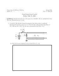
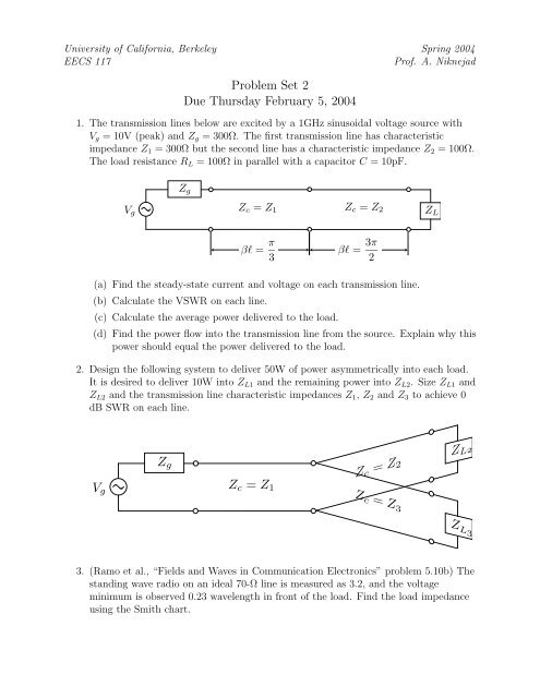
University of California, Berkeley Spring 2004EECS 117Prof. A. NiknejadProblem Set 2Due Thursday February 5, 20041. The transmission lines below are excited by a 1GHz sinusoidal voltage source withV g = 10V (peak) and Z g = 300Ω. The first transmission line has characteristicimpedance Z 1 = 300Ω but the second line has a characteristic impedance Z 2 = 100Ω.The load resistance R L = 100Ω in parallel with a capacitor C = 10pF.Z gβl = π 3V gZ c = Z 1Z c = Z 2Z Lβl = 3π 2(a) Find the steady-state current and voltage on each transmission line.(b) Calculate the VSWR on each line.(c) Calculate the average power delivered to the load.(d) Find the power flow into the transmission line from the source. Explain why thispower should equal the power delivered to the load.2. Design the following system to deliver 50W of power asymmetrically into each load.It is desired to deliver 10W into Z L1 and the remaining power into Z L2 . Size Z L1 andZ L2 and the transmission line characteristic impedances Z 1 , Z 2 and Z 3 to achieve 0dB SWR on each line.V gZ gZ c = Z 1Z c = Z 2 Z L2Z c = Z 3 Z L33. (Ramo et al., “Fields and Waves in Communication Electronics” problem 5.10b) Thestanding wave radio on an ideal 70-Ω line is measured as 3.2, and the voltageminimum is observed 0.23 wavelength in front of the load. Find the load impedanceusing the Smith chart.

4. (Collin, “Foundations of Microwave Engineering” problem 4.11) For the followingmicrowave circuit, evaluate the power transmitted to the load Z L . Find thestanding-wave ratio in the two transmission-line sections. Assume Z g = Z 1 , Z L = 2Z 1 ,X 1 = X 2 = Z 1 , V g = 5V (peak). Repeat your calculation with the Smith Chart.Z gZ c = Z 1V gZ c = Z 1jX 1jX 2Z Lβl = π 4βl = 3π 45. Consider a lossy RC line shown below. This is a physical model for a circuit wherethe series loss R ′ ≫ ωL ′ dominates over the inductance of the line. The particularexample is for an 1MΩ IC resistor with parasitic capacitance of 100fF with lengthl = 500µm.C ′ R ′ C ′ R ′ C ′ R ′ C ′ R ′(a) Using the general distributed circuit analyzed in class, find the propagationconstant and velocity for the line.(b) Find the input impedance for an arbitrary termination.(c) Show that the shorted line looks like a resistor at low frequency. What’s thepole frequency? How does it compare to a 1-section lumped approximation tothe line.(d) Show that the open line looks like a lossy capacitor at low frequency. What’sthe equivalent series resistance of the capacitor? How does it compare to a1-section lumped approximation to the line.(e) Plot the normalized voltage along the shorted line at a frequency of 1GHz.Compare the plot to an ideal resistor.2