Chapter 06 - Changing Education Paradigm

Contents
6 Mining Association Rules in Large Databases 3
6.1 Association rule mining . . . . . . . . . . . . . . . . . . . . . . . . . . . . . . . . . . . . . . . . . . . . 3
6.1.1 Market basket analysis: A motivating example for association rule mining . . . . . . . . . . . . 3
6.1.2 Basic concepts . . . . . . . . . . . . . . . . . . . . . . . . . . . . . . . . . . . . . . . . . . . . . 4
6.1.3 Association rule mining: A road map . . . . . . . . . . . . . . . . . . . . . . . . . . . . . . . . . 5
6.2 Mining single-dimensional Boolean association rules from transactional databases . . . . . . . . . . . . 6
6.2.1 The Apriori algorithm: Finding frequent itemsets . . . . . . . . . . . . . . . . . . . . . . . . . . 6
6.2.2 Generating association rules from frequent itemsets . . . . . . . . . . . . . . . . . . . . . . . . . 9
6.2.3 Variations of the Apriori algorithm . . . . . . . . . . . . . . . . . . . . . . . . . . . . . . . . . . 10
6.3 Mining multilevel association rules from transaction databases . . . . . . . . . . . . . . . . . . . . . . 12
6.3.1 Multilevel association rules . . . . . . . . . . . . . . . . . . . . . . . . . . . . . . . . . . . . . . 12
6.3.2 Approaches to mining multilevel association rules . . . . . . . . . . . . . . . . . . . . . . . . . . 14
6.3.3 Checking for redundant multilevel association rules . . . . . . . . . . . . . . . . . . . . . . . . . 16
6.4 Mining multidimensional association rules from relational databases and data warehouses . . . . . . . 17
6.4.1 Multidimensional association rules . . . . . . . . . . . . . . . . . . . . . . . . . . . . . . . . . . 17
6.4.2 Mining multidimensional association rules using static discretization of quantitative attributes 18
6.4.3 Mining quantitative association rules . . . . . . . . . . . . . . . . . . . . . . . . . . . . . . . . . 19
6.4.4 Mining distance-based association rules . . . . . . . . . . . . . . . . . . . . . . . . . . . . . . . 21
6.5 From association mining to correlation analysis . . . . . . . . . . . . . . . . . . . . . . . . . . . . . . . 23
6.5.1 Strong rules are not necessarily interesting: An example . . . . . . . . . . . . . . . . . . . . . . 23
6.5.2 From association analysis to correlation analysis . . . . . . . . . . . . . . . . . . . . . . . . . . 23
6.6 Constraint-based association mining . . . . . . . . . . . . . . . . . . . . . . . . . . . . . . . . . . . . . 24
6.6.1 Metarule-guided mining of association rules . . . . . . . . . . . . . . . . . . . . . . . . . . . . . 25
6.6.2 Mining guided by additional rule constraints . . . . . . . . . . . . . . . . . . . . . . . . . . . . 26
6.7 Summary . . . . . . . . . . . . . . . . . . . . . . . . . . . . . . . . . . . . . . . . . . . . . . . . . . . . 29
1

2 CONTENTS

c J. Han and M. Kamber, 1998, DRAFT!! DO NOT COPY!! DO NOT DISTRIBUTE!! September 15, 1999
Chapter 6
Mining Association Rules in Large
Databases
Association rule mining nds interesting association or correlation relationships among a large set of data items.
With massive amounts of data continuously being collected and stored in databases, many industries are becoming
interested in mining association rules from their databases. For example, the discovery of interesting association
relationships among huge amounts of business transaction records can help catalog design, cross-marketing, lossleader
analysis, and other business decision making processes.
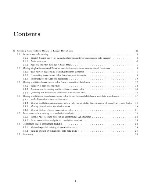
Atypical example of association rule mining is market basket analysis. This process analyzes customer buying
habits by nding associations between the di erent items that customers place in their \shopping baskets" (Figure
6.1). The discovery of such associations can help retailers develop marketing strategies by gaining insight into which
items are frequently purchased together by customers. For instance, if customers are buying milk, how likely are
they to also buy bread (and what kind of bread) on the same trip to the supermarket? Such information can lead to
increased sales by helping retailers to do selective marketing and plan their shelf space. For instance, placing milk
and bread within close proximity may further encourage the sale of these items together within single visits to the
store.
How can we nd association rules from large amounts of data, where the data are either transactional or relational?
Which association rules are the most interesting? How can we help or guide the mining procedure to discover
interesting associations? What language constructs are useful in de ning a data mining query language for association
rule mining? In this chapter, we will delve into each of these questions.
6.1 Association rule mining
Association rule mining searches for interesting relationships among items in a given data set. This section provides an
introduction to association rule mining. We begin in Section 6.1.1 by presenting an example of market basket analysis,
the earliest form of association rule mining. The basic concepts of mining associations are given in Section 6.1.2.
Section 6.1.3 presents a road map to the di erent kinds of association rules that can be mined.
6.1.1 Market basket analysis: A motivating example for association rule mining
Suppose, as manager of an AllElectronics branch, you would like to learn more about the buying habits of your
customers. Speci cally, you wonder \Which groups or sets of items are customers likely to purchase on a given trip
to the store?". To answer your question, market basket analysis may be performed on the retail data of customer
transactions at your store. The results may be used to plan marketing or advertising strategies, as well as catalog
design. For instance, market basket analysis may help managers design di erent store layouts. In one strategy, items
that are frequently purchased together can be placed in close proximity in order to further encourage the sale of such
items together. If customers who purchase computers also tend to buy nancial management software at the same
time, then placing the hardware display close to the software display may help to increase the sales of both of these
3

4 CHAPTER 6. MINING ASSOCIATION RULES IN LARGE DATABASES
Market analyst
Hmmm, which items are frequently
purchased together by my customers?
milk cereal
bread
milk eggs
bread
sugar
bread
butter
milk
Customer 1
Customer 2 Customer 3
SHOPPING BASKETS
Figure 6.1: Market basket analysis.
...
...
sugar eggs
Customer n
items. In an alternative strategy, placing hardware and software at opposite ends of the store may entice customers
who purchase such items to pick up other items along the way. For instance, after deciding on an expensive computer,
a customer may observe security systems for sale while heading towards the software display to purchase nancial
management software, and may decide to purchase a home security system as well. Market basket analysis can also
help retailers to plan which items to put on sale at reduced prices. If customers tend to purchase computers and
printers together, then having a sale on printers may encourage the sale of printers as well as computers.
If we think of the universe as the set of items available at the store, then each item has a Boolean variable
representing the presence or absence of that item. Each basket can then be represented by a Boolean vector of values
assigned to these variable. The Boolean vectors can be analyzed for buying patterns which re ect items that are
frequent associated or purchased together. These patterns can be represented in the form of association rules. For
example, the information that customers who purchase computers also tend to buy nancial management software
at the same time is represented in association Rule (6.1) below.
computer ) nancial management software [support =2%; confidence = 60%] (6.1)
Rule support and con dence are two measures of rule interestingness that were described earlier in Section 1.5.
They respectively re ect the usefulness and certainty of discovered rules. A support of 2% for association Rule (6.1)
means that 2% of all the transactions under analysis show that computer and nancial management software are
purchased together. A con dence of 60% means that 60% of the customers who purchased a computer also bought the
software. Typically, association rules are considered interesting if they satisfy both a minimum support threshold
and a minimum con dence threshold. Such thresholds can be set by users or domain experts.
6.1.2 Basic concepts
Let I=fi1, i2, :::, img be a set of items. Let D, the task relevant data, be a set of database transactions where each
transaction T is a set of items such that T I. Each transaction is associated with an identi er, called TID. Let A
be a set of items. A transaction T is said to contain A if and only if A T .Anassociation rule is an implication
of the form A ) B, where A I,B Iand A \ B = . The rule A ) B holds in the transaction set D with
support s, where s is the percentage of transactions in D that contain A [ B. The rule A ) B has con dence c

6.1. ASSOCIATION RULE MINING 5
in the transaction set D if c is the percentage of transactions in D containing A which also contain B. That is,
support(A ) B) = ProbfA[Bg (6.2)
confidence(A ) B) = ProbfBjAg: (6.3)
Rules that satisfy both a minimum support threshold (min sup) and a minimum con dence threshold (min conf) are
called strong.
A set of items is referred to as an itemset. An itemset that contains k items is a k-itemset. The set fcomputer,
nancial management softwareg is a 2-itemset. The occurrence frequency of an itemset is the number of
transactions that contain the itemset. This is also known, simply, as the frequency or support count of the
itemset. An itemset satis es minimum support if the occurrence frequency of the itemset is greater than or equal to
the product of min sup and the total number of transactions in D. If an itemset satis es minimum support, then it
is a frequent itemset 1 . The set of frequent k-itemsets is commonly denoted by Lk 2 .
\How are association rules mined from large databases?" Association rule mining is a two-step process:
Step 1: Find all frequent itemsets. By de nition, each of these itemsets will occur at least as frequently as a
pre-determined minimum support count.
Step 2: Generate strong association rules from the frequent itemsets. By de nition, these rules must satisfy
minimum support and minimum con dence.
Additional interestingness measures can be applied, if desired. The second step is the easiest of the two. The overall
performance of mining association rules is determined by the rst step.
6.1.3 Association rule mining: A road map
Market basket analysis is just one form of association rule mining. In fact, there are many kinds of association rules.
Association rules can be classi ed in various ways, based on the following criteria:
1. Based on the types of values handled in the rule:
If a rule concerns associations between the presence or absence of items, it is a Boolean association rule.
For example, Rule (6.1) above is a Boolean association rule obtained from market basket analysis.
If a rule describes associations between quantitative items or attributes, then it is a quantitative association
rule. In these rules, quantitative values for items or attributes are partitioned into intervals. Rule (6.4) below
is an example of a quantitative association rule.
age(X; \30 , 34") ^ income(X; \42K , 48K") ) buys(X ; \high resolution TV ") (6.4)
Note that the quantitative attributes, age and income, have been discretized.
2. Based on the dimensions of data involved in the rule:
If the items or attributes in an association rule each reference only one dimension, then it is a singledimensional
association rule. Note that Rule (6.1) could be rewritten as
buys(X ; \computer") ) buys(X ; \ nancial management software") (6.5)
Rule (6.1) is therefore a single-dimensional association rule since it refers to only one dimension, i.e., buys.
If a rule references two or more dimensions, such as the dimensions buys, time of transaction, and customer
category, then it is a multidimensional association rule. Rule (6.4) above is considered a multidimensional
association rule since it involves three dimensions, age, income, and buys.
1 In early work, itemsets satisfying minimum support were referred to as large. This term, however, is somewhat confusing as it has
connotations to the number of items in an itemset rather than the frequency of occurrence of the set. Hence, we use the more recent
term of frequent.
2 Although the term frequent is preferred over large, for historical reasons frequent k-itemsets are still denoted as Lk .

6 CHAPTER 6. MINING ASSOCIATION RULES IN LARGE DATABASES
3. Based on the levels of abstractions involved in the rule set:
Some methods for association rule mining can nd rules at di ering levels of abstraction. For example, suppose
that a set of association rules mined included Rule (6.6) and (6.7) below.
age(X; \30 , 34") ) buys(X ; \laptop computer") (6.6)
age(X; \30 , 34") ) buys(X ; \computer") (6.7)
In Rules (6.6) and (6.7), the items bought are referenced at di erent levels of abstraction. (That is, \computer"
is a higher level abstraction of \laptop computer"). We refer to the rule set mined as consisting of multilevel
association rules. If, instead, the rules within a given set do not reference items or attributes at di erent
levels of abstraction, then the set contains single-level association rules.
4. Based on the nature of the association involved in the rule: Association mining can be extended to correlation
analysis, where the absence or presence of correlated items can be identi ed.
Throughout the rest of this chapter, you will study methods for mining each of the association rule types described.
6.2 Mining single-dimensional Boolean association rules from transactional databases
In this section, you will learn methods for mining the simplest form of association rules - single-dimensional, singlelevel,
Boolean association rules, such as those discussed for market basket analysis in Section 6.1.1. We begin by
presenting Apriori, a basic algorithm for nding frequent itemsets (Section 6.2.1). A procedure for generating strong
association rules from frequent itemsets is discussed in Section 6.2.2. Section 6.2.3 describes several variations to the
Apriori algorithm for improved e ciency and scalability.
6.2.1 The Apriori algorithm: Finding frequent itemsets
Apriori is an in uential algorithm for mining frequent itemsets for Boolean association rules. The name of the
algorithm is based on the fact that the algorithm uses prior knowledge of frequent itemset properties, as we shall
see below. Apriori employs an iterative approach known as a level-wise search, where k-itemsets are used to explore
(k+1)-itemsets. First, the set of frequent 1-itemsets is found. This set is denoted L1. L1 is used to nd L2, the
frequent 2-itemsets, which is used to nd L3, and so on, until no more frequent k-itemsets can be found. The nding
of each Lk requires one full scan of the database.
To improve the e ciency of the level-wise generation of frequent itemsets, an important property called the
Apriori property, presented below, is used to reduce the search space.
The Apriori property. All non-empty subsets of a frequent itemset must also be frequent.
This property is based on the following observation. By de nition, if an itemset I does not satisfy the minimum
support threshold, s, then I is not frequent, i.e., ProbfIg

6.2. MINING SINGLE-DIMENSIONAL BOOLEAN ASSOCIATION RULES FROM TRANSACTIONAL DATABASES7
2. The prune step: Ck is a superset of Lk, that is, its members may ormay not be frequent, but all of the
frequent k-itemsets are included in Ck. A scan of the database to determine the count of each candidate in Ck
would result in the determination of Lk (i.e., all candidates having a count no less than the minimum support
count are frequent by de nition, and therefore belong to Lk). Ck, however, can be huge, and so this could
involve heavy computation. To reduce the size of Ck, the Apriori property is used as follows. Any (k-1)-itemset
that is not frequent cannot be a subset of a frequent k-itemset. Hence, if any (k-1)-subset of a candidate
k-itemset is not in Lk,1, then the candidate cannot be frequent either and so can be removed from Ck. This
subset testing can be done quickly by maintaining a hash tree of all frequent itemsets.
AllElectronics database
TID List of item ID's
T100 I1, I2, I5
T200 I2, I3, I4
T300 I3, I4
T400 I1, I2, I3, I4
Figure 6.2: Transactional data for an AllElectronics branch.
Example 6.1 Let's look at a concrete example of Apriori, based on the AllElectronics transaction database, D, of
Figure 6.2. There are four transactions in this database, i.e., jDj = 4. Apriori assumes that items within a transaction
are sorted in lexicographic order. We use Figure 6.3 to illustrate the APriori algorithm for nding frequent itemsets
in D.
In the rst iteration of the algorithm, each item is a member of the set of candidate 1-itemsets, C1. The
algorithm simply scans all of the transactions in order to count the number of occurrences of each item.
Suppose that the minimum transaction support count required is 2 (i.e., min sup = 50%). The set of frequent
1-itemsets, L1, can then be determined. It consists of the candidate 1-itemsets having minimum support.
To discover the set of frequent 2-itemsets, L2, the algorithm uses L1 1 L1 to generate a candidate set of
2-itemsets, C2 3 . C2 consists of , jL1j
2-itemsets.
2
Next, the transactions in D are scanned and the support count of each candidate itemset in C2 is accumulated,
as shown in the middle table of the second row in Figure 6.3.
The set of frequent 2-itemsets, L2, is then determined, consisting of those candidate 2-itemsets in C2 having
minimum support.
The generation of the set of candidate 3-itemsets, C3, is detailed in Figure 6.4. First, let C3 = L2 1 L2 =
ffI1;I2;I3g;fI1;I2;I4g;fI2;I3;I4gg. Based on the Apriori property that all subsets of a frequent itemset
must also be frequent, we can determine that the candidates fI1,I2,I3g and fI1,I2,I4g cannot possibly be
frequent. We therefore remove them from C3, thereby saving the e ort of unnecessarily obtaining their counts
during the subsequent scan of D to determine L3. Note that since the Apriori algorithm uses a level-wise search
strategy, then given a k-itemset, we only need to check if its (k-1)-subsets are frequent.
The transactions in D are scanned in order to determine L3, consisting of those candidate 3-itemsets in C3
having minimum support (Figure 6.3).
No more frequent itemsets can be found (since here, C4 = ), and so the algorithm terminates, having found
all of the frequent itemsets.
3 L1 1 L1 is equivalent toL1 L1 since the de nition of L k 1 L k requires the two joining itemsets to share k , 1 = 0 items.
2

8 CHAPTER 6. MINING ASSOCIATION RULES IN LARGE DATABASES
Scan D for
count of each
candidate
,!
Generate C2
candidates from
L1
,!
Generate C3
candidates from
L2
,!
C3
C2
Itemset
fI1,I2g
fI1,I3g
fI1,I4g
fI2,I3g
fI2,I4g
fI3,I4g
Itemset
fI2,I3,I4g
C1
Itemset Sup.
fI1g 2
fI2g 3
fI3g 3
fI4g 3
fI5g 1
Scan D for
count of each
candidate
,!
Scan D for
count of
each candidate
,!
C3
Itemset Sup.
fI2,I3,I4g 2
Compare candidate
support with
minimum support
count
,!
C2
Itemset Sup.
fI1,I2g 2
fI1,I3g 1
fI1,I4g 1
fI2,I3g 2
fI2,I4g 2
fI3,I4g 3
Compare candidate
support with
minimum support
count
,!
Compare candidate
support with
minimum support
count
,!
L1
Itemset Sup.
fI1g 2
fI2g 3
fI3g 3
fI4g 3
L2
Itemset Sup.
fI1,I2g 2
fI2,I3g 2
fI2,I4g 2
fI3,I4g 3
L3
Itemset Sup.
fI2,I3,I4g 2
Figure 6.3: Generation of candidate itemsets and frequent itemsets, where the minimum support count is2.
1. C3 = L2 1 L2 = ffI1,I2g, fI2,I3g, fI2,I4g, fI3,I4gg 1 ffI1,I2g, fI2,I3g, fI2,I4g, fI3,I4gg =
ffI1;I2;I3g;fI1;I2;I4g;fI2;I3;I4gg.
2. Apriori property: All subsets of a frequent itemset must also be frequent. Do any of the candidates have a
subset that is not frequent?
{ The 2-item subsets of fI1,I2,I3g are fI1,I2g, fI1,I3g, and fI2,I3g. fI1,I3g is not a member of L2, and so
it is not frequent. Therefore, remove fI1,I2,I3g from C3.
{ The 2-item subsets of fI1,I2,I4g are fI1,I2g, fI1,I4g, and fI2,I4g. fI1,I4g is not a member of L2, and so
it is not frequent. Therefore, remove fI1,I2,I4g from C3.
{ The 2-item subsets of fI2,I3,I4g are fI2,I3g, fI2,I4g, and fI3,I4g. All 2-item subsets of fI2,I3,I4g are
members of L2. Therefore, keep fI2,I3,I4g in C3.
3. Therefore, C3 = ffI2;I3;I4gg.
Figure 6.4: Generation of candidate 3-itemsets, C3, from L2 using the Apriori property.

6.2. MINING SINGLE-DIMENSIONAL BOOLEAN ASSOCIATION RULES FROM TRANSACTIONAL DATABASES9
Algorithm 6.2.1 (Apriori) Find frequent itemsets using an iterative level-wise approach.
Input: Database, D, of transactions; minimum support threshold, min sup.
Output: L, frequent itemsets in D.
Method:
1) L1 = nd frequent 1-itemsets(D);
2) for (k =2;L k,16= ;k++) f
3) C k = apriori gen(Lk,1, min sup);
4) for each transaction t 2 D f // scan D for counts
5) C t = subset(Ck ;t); // get the subsets of t that are candidates
6) for each candidate c 2 C t
7) c.count++;
8) g
9) L k = fc 2 Ckjc:count min supg
10) g
11) return L = [ kLk;
procedure apriori gen(L k,1:frequent (k-1)-itemsets; min sup: minimum support)
1) for each itemset l1 2 L k,1
2) for each itemset l2 2 Lk,1
3) if (l1[1] = l2[1]) ^ (l1[2] = l2[2]) ^ ::: ^ (l1[k , 2] = l2[k , 2]) ^ (l1[k , 1]

10 CHAPTER 6. MINING ASSOCIATION RULES IN LARGE DATABASES
con dence). This can be done using Equation (6.8) for con dence, where the conditional probability is expressed in
terms of itemset support:
support(A [ B)
confidence(A ) B) =Prob(BjA)= ; (6.8)
support(A)
where support(A [ B) is the number of transactions containing the itemsets A [ B, and support(A) is the number
of transactions containing the itemset A.
Based on this equation, association rules can be generated as follows.
For each frequent itemset, l, generate all non-empty subsets of l.
For every non-empty subset s, ofl, output the rule \s ) (l , s)" if support(l)
support(s)
the minimum con dence threshold.
min conf, where min conf is
Since the rules are generated from frequent itemsets, then each one automatically satis es minimum support. Frequent
itemsets can be stored ahead of time in hash tables along with their counts so that they can be accessed
quickly.
Example 6.2 Let's try an example based on the transactional data for AllElectronics shown in Figure 6.2. Suppose
the data contains the frequent itemset l = fI2,I3,I4g. What are the association rules that can be generated from l?
The non-empty subsets of l are fI2,I3g, fI2,I4g, fI3,I4g, fI2g, fI3g, and fI4g. The resulting association rules are as
shown below, each listed with its con dence.
I2 ^ I3 ) I4, confidence =2=2 = 100%
I2 ^ I4 ) I3, confidence =2=2 = 100%
I3 ^ I4 ) I2, confidence =2=3 = 67%
I2 ) I3 ^ I4, confidence =2=3 = 67%
I3 ) I2 ^ I4, confidence =2=3 = 67%
I4 ) I2 ^ I3, confidence =2=3 = 67%
If the minimum con dence threshold is, say, 70%, then only the rst and second rules above are output, since these
are the only ones generated that are strong. 2
6.2.3 Variations of the Apriori algorithm
\How might the e ciency of Apriori be improved?"
Many variations of the Apriori algorithm have been proposed. A number of these variations are enumerated
below. Methods 1 to 6 focus on improving the e ciency of the original algorithm, while methods 7 and 8 consider
transactions over time.
1. A hash-based technique: Hashing itemset counts.
A hash-based technique can be used to reduce the size of the candidate k-itemsets, Ck, for k>1. For example,
when scanning each transaction in the database to generate the frequent 1-itemsets, L1, from the candidate
1-itemsets in C1, we can generate all of the 2-itemsets for each transaction, hash (i.e., map) them into the
di erent buckets of a hash table structure, and increase the corresponding bucket counts (Figure 6.6). A 2itemset
whose corresponding bucket count in the hash table is below the support threshold cannot be frequent
and thus should be removed from the candidate set. Such a hash-based technique may substantially reduce
the number of the candidate k-itemsets examined (especially when k = 2).
2. Scan reduction: Reducing the number of database scans.
Recall that in the Apriori algorithm, one scan is required to determine Lk for each Ck. A scan reduction
technique reduces the total number of scans required by doing extra work in some scans. For example, in the
Apriori algorithm, C3 is generated based on L2 1 L2. However, C2 can also be used to generate the candidate
3-itemsets. Let C0 3 be the candidate 3-itemsets generated from C2 1 C2, instead of from L2 1 L2. Clearly, jC0 3j will be greater than jC3j. However, if jC0 3j is not much larger than jC3j, and both C2 and C0 3 can be stored in

6.2. MINING SINGLE-DIMENSIONAL BOOLEAN ASSOCIATION RULES FROM TRANSACTIONAL DATABASES11
Create hash table, H2
using hash function
h(x; y) =((order of x) 10
+(order of y)) mod 7
,!
H2
bucket address 0 1 2 3 4 5 6
bucket count 1 1 2 2 1 2 4
bucket contents fI1,I4g fI1,I5g fI2,I3g fI2,I4g fI2,I5g fI1,I2g fI3,I4g
fI2,I3g fI2,I4g fI1,I2g fI3,I4g
fI1,I3g
fI3,I4g
Figure 6.6: Hash table, H2, for candidate 2-itemsets: This hash table was generated by scanning the transactions
of Figure 6.2 while determining L1 from C1. If the minimum support count is 2, for example, then the itemsets in
buckets 0, 1, and 4 cannot be frequent and so they should not be included in C2.
main memory,we can nd L2 and L3 together when the next scan of the database is performed, thereby saving
one database scan. Using this strategy, we can determine all Lk's by as few as two scans of the database (i.e.,
one initial scan to determine L1 and a nal scan to determine all other large itemsets), assuming that C 0
k for
k 3 is generated from C0 k,1 and all C0
ks for k>2 can be kept in the memory.
3. Transaction reduction: Reducing the number of transactions scanned in future iterations.
A transaction which does not contain any frequent k-itemsets cannot contain any frequent (k+ 1)-itemsets.
Therefore, such a transaction can be marked or removed from further consideration since subsequent scans of
the database for j-itemsets, where j>k, will not require it.
4. Partitioning: Partitioning the data to nd candidate itemsets.
A partitioning technique can be used which requires just two database scans to mine the frequent itemsets
(Figure 6.7). It consists of two phases. In Phase I, the algorithm subdivides the transactions of D into n
non-overlapping partitions. If the minimum support threshold for transactions in D is min sup, then the
minimum itemset support count for a partition is min sup the number of transactions in that partition. For
each partition, all frequent itemsets within the partition are found. These are referred to as local frequent
itemsets. The procedure employs a special data structure which, for each itemset, records the TID's of the
transactions containing the items in the itemset. This allows it to nd all of the local frequent k-itemsets, for
k =1;2;:::, in just one scan of the database.
A local frequent itemset may ormay not be frequent with respect to the entire database, D. Any itemset
that is potentially frequent with respect to D must occur as a frequent itemset in at least one of the partitions.
Therefore, all local frequent itemsets are candidate itemsets with respect to D. The collection of frequent
itemsets from all partitions forms a global candidate itemset with respect to D. In Phase II, a second scan
of D is conducted in which the actual support of each candidate is assessed in order to determine the global
frequent itemsets. Partition size and the number of partitions are set so that each partition can t into main
memory and therefore be read only once in each phase.
Transactions
in D
Divided D into
n partitions
PHASE I
Find the frequent
itemsets local to
each partition
(1 scan)
5. Sampling: Mining on a subset of the given data.
Combine all
local frequent
itemsets to form
candidate itemset
Figure 6.7: Mining by partitioning the data.
PHASE II
Find global
frequent itemsets
among candidates
(1 scan)
Frequent
itemsets in D

12 CHAPTER 6. MINING ASSOCIATION RULES IN LARGE DATABASES
The basic idea of the sampling approach istopick a random sample S of the given data D, and then search
for frequent itemsets in S instead D. In this way, we trade o some degree of accuracy against e ciency. The
sample size of S is such that the search for frequent itemsets in S can be done in main memory, and so, only
one scan of the transactions in S is required overall. Because we are searching for frequent itemsets in S rather
than in D, it is possible that we will miss some of the global frequent itemsets. To lessen this possibility, we
use a lower support threshold than minimum support to nd the frequent itemsets local to S (denoted L S ).
The rest of the database is then used to compute the actual frequencies of each itemset in L S . A mechanism
is used to determine whether all of the global frequent itemsets are included in L S . If L S actually contained
all of the frequent itemsets in D, then only one scan of D was required. Otherwise, a second pass can be done
in order to nd the frequent itemsets that were missed in the rst pass. The sampling approach is especially
bene cial when e ciency is of utmost importance, such as in computationally intensive applications that must
be run on a very frequent basis.
6. Dynamic itemset counting: Adding candidate itemsets at di erent points during a scan.
A dynamic itemset counting technique was proposed in which the database is partitioned into blocks marked by
start points. In this variation, new candidate itemsets can be added at any start point, unlike in Apriori, which
determines new candidate itemsets only immediately prior to each complete database scan. The technique
is dynamic in that it estimates the support of all of the itemsets that have been counted so far, adding new
candidate itemsets if all of their subsets are estimated to be frequent. The resulting algorithm requires two
database scans.
7. Calendric market basket analysis: Finding itemsets that are frequent in a set of user-de ned time intervals.
Calendric market basket analysis uses transaction time stamps to de ne subsets of the given database. An
itemset that does not satisfy minimum support may be considered frequent with respect to a subset of the
database which satis es user-speci ed time constraints.
8. Sequential patterns: Finding sequences of transactions associated over time.
The goal of sequential pattern analysis is to nd sequences of itemsets that many customers have purchased in
roughly the same order. A transaction sequence is said to contain an itemset sequence if each itemset is
contained in one transaction, and the following condition is satis ed: If the ith itemset in the itemset sequence
is contained in transaction j in the transaction sequence, then the (i + 1)th itemset in the itemset sequence is
contained in a transaction numbered greater than j. The support of an itemset sequence is the percentage of
transaction sequences that contain it.
Other variations involving the mining of multilevel and multidimensional association rules are discussed in the
rest of this chapter. The mining of time sequences is further discussed in Chapter 9.
6.3 Mining multilevel association rules from transaction databases
6.3.1 Multilevel association rules
For many applications, it is di cult to nd strong associations among data items at low or primitive levels of
abstraction due to the sparsity of data in multidimensional space. Strong associations discovered at very high
concept levels may represent common sense knowledge. However, what may represent common sense to one user,
may seem novel to another. Therefore, data mining systems should provide capabilities to mine association rules at
multiple levels of abstraction and traverse easily among di erent abstraction spaces.
Let's examine the following example.
Example 6.3 Suppose we are given the task-relevant set of transactional data in Table 6.1 for sales at the computer
department ofanAllElectronics branch, showing the items purchased for each transaction TID. The concept hierarchy
for the items is shown in Figure 6.8. A concept hierarchy de nes a sequence of mappings from a set of low level
concepts to higher level, more general concepts. Data can be generalized by replacing low level concepts within the
data by their higher level concepts, or ancestors, from a concept hierarchy 4 . The concept hierarchy of Figure 6.8 has
4 Concept hierarchies were described in detail in Chapters 2 and 4. In order to make the chapters of this book as self-contained as
possible, we o er their de nition again here. Generalization was described in Chapter 5.

6.3. MINING MULTILEVEL ASSOCIATION RULES FROM TRANSACTION DATABASES 13
computer
software
all(computer items)
printer
home laptop educational financial
management
color b/w
IBM Microsoft HP Epson Canon
Ergoway
wrist
pad
Figure 6.8: A concept hierarchy for AllElectronics computer items.
computer
accessory
mouse
Logitech
four levels, referred to as levels 0, 1, 2, and 3. By convention, levels within a concept hierarchy are numbered from top
to bottom, starting with level 0 at the root node for all (the most general abstraction level). Here, level 1 includes
computer, software, printer and computer accessory, level 2 includes home computer, laptop computer, education
software, nancial management software, .., and level 3 includes IBM home computer, .., Microsoft educational
software, and so on. Level 3 represents the most speci c abstraction level of this hierarchy. Concept hierarchies may
be speci ed by users familiar with the data, or may exist implicitly in the data.
TID Items Purchased
1 IBM home computer, Sony b/w printer
2 Microsoft educational software, Microsoft nancial management software
3 Logitech mouse computer-accessory, Ergo-way wrist pad computer-accessory
4 IBM home computer, Microsoft nancial management software
5 IBM home computer
... ...
Table 6.1: Task-relevant data, D.
The items in Table 6.1 are at the lowest level of the concept hierarchy of Figure 6.8. It is di cult to nd interesting
purchase patterns at such raw or primitive level data. For instance, if \IBM home computer" or \Sony b/w (black
and white) printer" each occurs in a very small fraction of the transactions, then it may be di cult to nd strong
associations involving such items. Few people may buy such items together, making it is unlikely that the itemset
\fIBM home computer, Sony b/w printerg" will satisfy minimum support. However, consider the generalization
of \Sony b/w printer" to \b/w printer". One would expect that it is easier to nd strong associations between
\IBM home computer" and \b/w printer" rather than between \IBM home computer" and \Sony b/w printer".
Similarly, many people may purchase \computer" and \printer" together, rather than speci cally purchasing \IBM
home computer" and \Sony b/w printer" together. In other words, itemsets containing generalized items, such as
\fIBM home computers, b/w printerg" and \fcomputer, printerg" are more likely to have minimum support than
itemsets containing only primitive level data, such as\fIBM home computers, Sony b/w printerg". Hence, it is
easier to nd interesting associations among items at multiple concept levels, rather than only among low level data.
2
Rules generated from association rule mining with concept hierarchies are called multiple-level or multilevel

14 CHAPTER 6. MINING ASSOCIATION RULES IN LARGE DATABASES
level 1
min_sup = 5%
level 2
min_sup = 5%
level 1
min_sup = 5%
level 2
min_sup = 3%
laptop computer [support = 6%]
laptop computer [support = 6%]
computer [support = 10%]
home computer [support = 4%]
Figure 6.9: Multilevel mining with uniform support.
computer [support = 10%]
home computer [support = 4%]
Figure 6.10: Multilevel mining with reduced support.
association rules, since they consider more than one concept level.
6.3.2 Approaches to mining multilevel association rules
\How can we mine multilevel association rules e ciently using concept hierarchies?"
Let's look at some approaches based on a support-con dence framework. In general, a top-down strategy is
employed, where counts are accumulated for the calculation of frequent itemsets at each concept level, starting at
the concept level 1 and working towards the lower, more speci c concept levels, until no more frequent itemsets can
be found. That is, once all frequent itemsets at concept level 1 are found, then the frequent itemsets at level 2 are
found, and so on. For each level, any algorithm for discovering frequent itemsets may be used, such as Apriori or its
variations. A numberofvariations to this approach are described below, and illustrated in Figures 6.9 to 6.13, where
rectangles indicate an item or itemset that has been examined, and rectangles with thick borders indicate that an
examined item or itemset is frequent.
1. Using uniform minimum support for all levels (referred to as uniform support): The same minimum
support threshold is used when mining at each level of abstraction. For example, in Figure 6.9, a minimum
support threshold of 5% is used throughout (e.g., for mining from \computer" down to \laptop computer").
Both \computer" and \laptop computer" are found to be frequent, while \home computer" is not.
When a uniform minimum support threshold is used, the search procedure is simpli ed. The method is also
simple in that users are required to specify only one minimum support threshold. An optimization technique
can be adopted, based on the knowledge that an ancestor is a superset of its descendents: the search avoids
examining itemsets containing any item whose ancestors do not have minimum support.
The uniform support approach, however, has some di culties. It is unlikely that items at lower levels of
abstraction will occur as frequently as those at higher levels of abstraction. If the minimum support threshold is
set too high, it could miss several meaningful associations occurring at low abstraction levels. If the threshold is
level 1
min_sup = 12%
level 2
min_sup = 3%
laptop (not examined)
computer [support = 10%]
home computer (not examined)
Figure 6.11: Multilevel mining with reduced support, using level-cross ltering by a single item.

6.3. MINING MULTILEVEL ASSOCIATION RULES FROM TRANSACTION DATABASES 15
level 1
min_sup = 5%
level 2
min_sup = 2%
laptop computer &
b/w printer
[support = 1%]
computer & printer [support = 7%]
laptop computer &
color printer
[support = 2%]
home computer &
b/w printer
[support = 1%]
home computer &
color printer
[support = 3%]
Figure 6.12: Multilevel mining with reduced support, using level-cross ltering by ak-itemset. Here, k =2.
set too low, it may generate many uninteresting associations occurring at high abstraction levels. This provides
the motivation for the following approach.
2. Using reduced minimum support at lower levels (referred to as reduced support): Each level of
abstraction has its own minimum support threshold. The lower the abstraction level is, the smaller the corresponding
threshold is. For example, in Figure 6.10, the minimum support thresholds for levels 1 and 2 are 5%
and 3%, respectively. In this way, \computer", \laptop computer", and \home computer" are all considered
frequent.
For mining multiple-level associations with reduced support, there are a number of alternative search strategies.
These include:
1. level-by-level independent: This is a full breadth search, where no background knowledge of frequent
itemsets is used for pruning. Each node is examined, regardless of whether or not its parent node is found to
be frequent.
2. level-cross lteringby single item: An item at the i-th level is examined if and only if its parent nodeatthe
(i,1)-th level is frequent. In other words, we investigate a more speci c association from a more general one.
If a node is frequent, its children will be examined; otherwise, its descendents are pruned from the search. For
example, in Figure 6.11, the descendent nodes of \computer" (i.e., \laptop computer" and \home computer")
are not examined, since \computer" is not frequent.
3. level-cross ltering byk-itemset: Ak-itemset at the i-th level is examined if and only if its corresponding
parent k-itemset at the (i , 1)-th level is frequent. For example, in Figure 6.12, the 2-itemset \fcomputer,
printerg" is frequent, therefore the nodes \flaptop computer, b/w printerg", \flaptop computer, color printerg",
\fhome computer, b/w printerg", and \fhome computer, color printerg" are examined.
\How do these methods compare?"
The level-by-level independent strategy is very relaxed in that it may lead to examining numerous infrequent
items at low levels, nding associations between items of little importance. For example, if \computer furniture"
is rarely purchased, it may not be bene cial to examine whether the more speci c \computer chair" is associated
with \laptop". However, if \computer accessories" are sold frequently, itmay be bene cial to see whether there is
an associated purchase pattern between \laptop" and \mouse".
The level-cross ltering by k-itemset strategy allows the mining system to examine only the children of frequent
k-itemsets. This restriction is very strong in that there usually are not many k-itemsets (especially when k>2)
which, when combined, are also frequent. Hence, many valuable patterns may be ltered out using this approach.
The level-cross ltering by single item strategy represents a compromise between the two extremes. However,
this method may miss associations between low level items that are frequent based on a reduced minimum support,
but whose ancestors do not satisfy minimum support (since the support thresholds at each level can be di erent).
For example, if \color monitor" occurring at concept level i is frequent based on the minimum support threshold of
level i, but its parent \monitor" at level (i , 1) is not frequent according to the minimum support threshold of level
(i , 1), then frequent associations such as\home computer ) color monitor" will be missed.
A modi ed version of the level-cross ltering by single item strategy, known as the controlled level-cross
ltering by single item strategy, addresses the above concern as follows. A threshold, called the level passage

16 CHAPTER 6. MINING ASSOCIATION RULES IN LARGE DATABASES
level 1
min_sup = 12%
level_passage_sup = 8%
level 2
min_sup = 3%
.
laptop computer [support = 6%]
computer [support = 10%]
home computer [support = 4%]
Figure 6.13: Multilevel mining with controlled level-cross ltering by single item
threshold, can be set up for \passing down" relatively frequent items (called subfrequent items) tolower levels.
In other words, this method allows the children of items that do not satisfy the minimum support threshold to
be examined if these items satisfy the level passage threshold. Each concept level can have its own level passage
threshold. The level passage threshold for a given level is typically set to a value between the minimum support
threshold of the next lower level and the minimum support threshold of the given level. Users may choose to \slide
down" or lower the level passage threshold at high concept levels to allow the descendents of the subfrequent items
at lower levels to be examined. Sliding the level passage threshold down to the minimum support threshold of the
lowest level would allow the descendents of all of the items to be examined. For example, in Figure 6.13, setting the
level passage threshold (level passage sup) of level 1 to 8% allows the nodes \laptop computer" and \home computer"
at level 2 to be examined and found frequent, even though their parent node, \computer", is not frequent. By adding
this mechanism, users have the exibility to further control the mining process at multiple abstraction levels, as well
as reduce the number of meaningless associations that would otherwise be examined and generated.
So far, our discussion has focussed on nding frequent itemsets where all items within the itemset must belong to
the same concept level. This may result in rules such as\computer ) printer" (where \computer" and \printer"
are both at concept level 1) and \home computer ) b/w printer" (where \home computer" and \b/w printer" are
both at level 2 of the given concept hierarchy). Suppose, instead, that we would like to nd rules that cross concept
level boundaries, such as\computer ) b/w printer", where items within the rule are not required to belong to the
same concept level. These rules are called cross-level association rules.
\How can cross-level associations be mined?" If mining associations from concept levels i and j, where level j is
more speci c (i.e., at a lower abstraction level) than i, then the reduced minimum support threshold of level j should
be used overall so that items from level j can be included in the analysis.
6.3.3 Checking for redundant multilevel association rules
Concept hierarchies are useful in data mining since they permit the discovery of knowledge at di erent levels of
abstraction, such asmultilevel association rules. However, when multilevel association rules are mined, some of the
rules found will be redundant due to \ancestor" relationships between items. For example, consider Rules (6.9) and
(6.10) below, where \home computer" is an ancestor of \IBM home computer" based on the concept hierarchy of
Figure 6.8.
home computer ) b=w printer; [support =8%; confidence = 70%] (6.9)
IBM home computer ) b=w printer; [support =2%; confidence = 72%] (6.10)
\If Rules (6.9) and (6.10) are both mined, then how useful is the latter rule?", you may wonder. \Does it really
provide any novel information?"
If the latter, less general rule does not provide new information, it should be removed. Let's have alookathow
this may be determined. A rule R1 isanancestor of a rule R2 ifR1 can be obtained by replacing the items in R2 by
their ancestors in a concept hierarchy. For example, Rule (6.9) is an ancestor of Rule (6.10) since \home computer"
is an ancestor of \IBM home computer". Based on this de nition, a rule can be considered redundant if its support
and con dence are close to their \expected" values, based on an ancestor of the rule. As an illustration, suppose
that Rule (6.9) has a 70% con dence and 8% support, and that about one quarter of all \home computer" sales are
for \IBM home computers", and a quarter of all \printers" sales are \black/white printers" sales. One may expect

6.4. MINING MULTIDIMENSIONAL ASSOCIATION RULES FROM RELATIONAL DATABASES AND DATA WAREHOUSE
Rule (6.10) to have a con dence of around 70% (since all data samples of \IBM home computer" are also samples of
\home computer") and a support of 2% (i.e., 8% 1
). If this is indeed the case, then Rule (6.10) is not interesting
4
since it does not o er any additional information and is less general than Rule (6.9).
6.4 Mining multidimensional association rules from relational databases and data
warehouses
6.4.1 Multidimensional association rules
Up to this point in this chapter, we have studied association rules which imply a single predicate, that is, the predicate
buys. For instance, in mining our AllElectronics database, we may discover the Boolean association rule \IBM home
computer ) Sony b/w printer", which can also be written as
buys(X; \IBM home computer") ) buys(X; \Sony b=w printer"); (6.11)
where X is a variable representing customers who purchased items in AllElectronics transactions. Similarly, if
\printer" is a generalization of \Sony b/w printer", then a multilevel association rule like \IBM home computers
) printer" can be expressed as
buys(X; \IBM home computer") ) buys(X; \printer"): (6.12)
Following the terminology used in multidimensional databases, we refer to each distinct predicate in a rule as a
dimension. Hence, we can refer to Rules (6.11) and (6.12) as single-dimensional or intra-dimension association
rules since they each contain a single distinct predicate (e.g., buys) with multiple occurrences (i.e., the predicate
occurs more than once within the rule). As we have seen in the previous sections of this chapter, such rules are
commonly mined from transactional data.
Suppose, however, that rather than using a transactional database, sales and related information are stored
in a relational database or data warehouse. Such data stores are multidimensional, by de nition. For instance,
in addition to keeping track of the items purchased in sales transactions, a relational database may record other
attributes associated with the items, such as the quantity purchased or the price, or the branch location of the sale.
Addition relational information regarding the customers who purchased the items, such as customer age, occupation,
credit rating, income, and address, may also be stored. Considering each database attribute or warehouse dimension
as a predicate, it can therefore be interesting to mine association rules containing multiple predicates, such as
age(X; \19 , 24") ^ occupation(X; \student") ) buys(X; \laptop"): (6.13)
Association rules that involve two or more dimensions or predicates can be referred to as multidimensional association
rules. Rule (6.13) contains three predicates (age, occupation, and buys), each of which occurs only once in
the rule. Hence, we say that it has no repeated predicates. Multidimensional association rules with no repeated
predicates are called inter-dimension association rules. Wemay also be interested in mining multidimensional
association rules with repeated predicates, which contain multiple occurrences of some predicate. These rules are
called hybrid-dimension association rules. An example of such a rule is Rule (6.14), where the predicate buys
is repeated.
age(X; \19 , 24") ^ buys(X; \laptop") ) buys(X; \b=w printer"): (6.14)
Note that database attributes can be categorical or quantitative. Categorical attributes have a nite number
of possible values, with no ordering among the values (e.g., occupation, brand, color). Categorical attributes are also
called nominal attributes, since their values are \names of things". Quantitative attributes are numeric and have
an implicit ordering among values (e.g., age, income, price). Techniques for mining multidimensional association rules
can be categorized according to three basic approaches regarding the treatment of quantitative (continuous-valued)
attributes.

18 CHAPTER 6. MINING ASSOCIATION RULES IN LARGE DATABASES
()
(age) (income) (buys)
(age, income) (age, buys) (income, buys)
(age, income, buys)
0-D (apex) cuboid; all
1-D cuboids
2-D cuboids
3-D (base) cuboid
Figure 6.14: Lattice of cuboids, making up a 3-dimensional data cube. Each cuboid represents a di erent group-by.
The base cuboid contains the three predicates, age, income, and buys.
1. In the rst approach, quantitative attributes are discretized using prede ned concept hierarchies. This discretization
occurs prior to mining. For instance, a concept hierarchy for income may be used to replace the
original numeric values of this attribute by ranges, such as\0-20K", \21-30K", \31-40K", and so on. Here,
discretization is static and predetermined. The discretized numeric attributes, with their range values, can then
be treated as categorical attributes (where each range is considered a category). We refer to this as mining
multidimensional association rules using static discretization of quantitative attributes.
2. In the second approach, quantitative attributes are discretized into \bins" based on the distribution of the data.
These bins may be further combined during the mining process. The discretization process is dynamic and
established so as to satisfy some mining criteria, such as maximizing the con dence of the rules mined. Because
this strategy treats the numeric attribute values as quantities rather than as prede ned ranges or categories,
association rules mined from this approach are also referred to as quantitative association rules.
3. In the third approach, quantitative attributes are discretized soastocapture the semantic meaning of such
interval data. This dynamic discretization procedure considers the distance between data points. Hence, such
quantitative association rules are also referred to as distance-based association rules.
Let's study each of these approaches for mining multidimensional association rules. For simplicity, we con ne our
discussion to inter-dimension association rules. Note that rather than searching for frequent itemsets (as is done
for single-dimensional association rule mining), in multidimensional association rule mining we search for frequent
predicatesets. A k-predicateset is a set containing k conjunctive predicates. For instance, the set of predicates
fage, occupation, buysg from Rule (6.13) is a 3-predicateset. Similar to the notation used for itemsets, we use the
notation Lk to refer to the set of frequent k-predicatesets.
6.4.2 Mining multidimensional association rules using static discretization of quantitative
attributes
Quantitative attributes, in this case, are discretized prior to mining using prede ned concept hierarchies, where
numeric values are replaced by ranges. Categorical attributes may also be generalized to higher conceptual levels if
desired.
If the resulting task-relevant data are stored in a relational table, then the Apriori algorithm requires just a slight
modi cation so as to nd all frequent predicatesets rather than frequent itemsets (i.e., by searching through all of
the relevant attributes, instead of searching only one attribute, like buys). Finding all frequent k-predicatesets will
require k or k + 1 scans of the table. Other strategies, such as hashing, partitioning, and sampling may be employed
to improve the performance.
Alternatively, the transformed task-relevant data may be stored in a data cube. Data cubes are well-suited for the
mining of multidimensional association rules, since they are multidimensional by de nition. Data cubes, and their
computation, were discussed in detail in Chapter 2. To review, a data cube consists of a lattice of cuboids which

6.4. MINING MULTIDIMENSIONAL ASSOCIATION RULES FROM RELATIONAL DATABASES AND DATA WAREHOUSE
are multidimensional data structures. These structures can hold the given task-relevant data, as well as aggregate,
group-by information. Figure 6.14 shows the lattice of cuboids de ning a data cube for the dimensions age, income,
and buys. The cells of an n-dimensional cuboid are used to store the counts, or support, of the corresponding npredicatesets.
The base cuboid aggregates the task-relevant data by age, income, and buys; the 2-D cuboid, (age,
income), aggregates by age and income; the 0-D (apex) cuboid contains the total number of transactions in the task
relevant data, and so on.
Due to the ever-increasing use of data warehousing and OLAP technology, it is possible that a data cube containing
the dimensions of interest to the user may already exist, fully materialized. \If this is the case, how can we go about
nding the frequent predicatesets?" A strategy similar to that employed in Apriori can be used, based on prior
knowledge that every subset of a frequent predicateset must also be frequent. This property can be used to reduce
the number of candidate predicatesets generated.
In cases where no relevant data cube exists for the mining task, one must be created. Chapter 2 describes
algorithms for fast, e cient computation of data cubes. These can be modi ed to search for frequent itemsets during
cube construction. Studies have shown that even when a cube must be constructed on the y, mining from data
cubes can be faster than mining directly from a relational table.
6.4.3 Mining quantitative association rules
Quantitative association rules are multidimensional association rules in which the numeric attributes are dynamically
discretized during the mining process so as to satisfy some mining criteria, such as maximizing the con dence or
compactness of the rules mined. In this section, we will focus speci cally on how to mine quantitative association rules
having two quantitative attributes on the left-hand side of the rule, and one categorical attribute on the right-hand
side of the rule, e.g.,
Aquan1 ^ Aquan2 ) Acat,
where Aquan1 and Aquan2 are tests on quantitative attribute ranges (where the ranges are dynamically determined),
and Acat tests a categorical attribute from the task-relevant data. Such rules have been referred to as
two-dimensional quantitative association rules, since they contain two quantitative dimensions. For instance,
suppose you are curious about the association relationship between pairs of quantitative attributes, like customer age
and income, and the type of television that customers like tobuy. An example of such a 2-D quantitative association
rule is
age(X; \30 , 34") ^ income(X; \42K , 48K") ) buys(X ; \high resolution TV ") (6.15)
\How can we nd such rules?" Let's look at an approach used in a system called ARCS (Association Rule
Clustering System) which borrows ideas from image-processing. Essentially, this approach maps pairs of quantitative
attributes onto a 2-D grid for tuples satisfying a given categorical attribute condition. The grid is then searched for
clusters of points, from which the association rules are generated. The following steps are involved in ARCS:
Binning. Quantitative attributes can have avery wide range of values de ning their domain. Just think about
how big a 2-D grid would be if we plotted age and income as axes, where each possible value of age was assigned
a unique position on one axis, and similarly, each possible value of income was assigned a unique position on the
other axis! To keep grids down to a manageable size, we instead partition the ranges of quantitative attributes into
intervals. These intervals are dynamic in that they may later be further combined during the mining process. The
partitioning process is referred to as binning, i.e., where the intervals are considered \bins". Three common binning
strategies are:
1. equi-width binning, where the interval size of each bin is the same,
2. equi-depth binning, where each bin has approximately the same number of tuples assigned to it, and
3. homogeneity-based binning, where bin size is determined so that the tuples in each bin are uniformly
distributed.
In ARCS, equi-width binning is used, where the bin size for each quantitative attribute is input by the user. A
2-D array for each possible bin combination involving both quantitative attributes is created. Each array cell holds

20 CHAPTER 6. MINING ASSOCIATION RULES IN LARGE DATABASES
.
income
70-80K
60-70K
50-60K
40-50K
30-40K
20-30K

6.4. MINING MULTIDIMENSIONAL ASSOCIATION RULES FROM RELATIONAL DATABASES AND DATA WAREHOUSE
Price ($) Equi-width Equi-depth Distance-based
(width $10) (depth $2)
7 [0, 10] [7, 20] [7, 7]
20 [11, 20] [22, 50] [20, 22]
22 [21, 30] [51, 53] [50, 53]
50 [31, 40]
51 [41, 50]
53 [51, 60]
Figure 6.16: Binning methods like equi-width and equi-depth do not always capture the semantics of interval data.
6.4.4 Mining distance-based association rules
The previous section described quantitative association rules where quantitative attributes are discretized initially
by binning methods, and the resulting intervals are then combined. Such an approach, however, may not capture the
semantics of interval data since they do not consider the relative distance between data points or between intervals.
Consider, for example, Figure 6.16 which shows data for the attribute price, partitioned according to equiwidth
and equi-depth binning versus a distance-based partitioning. The distance-based partitioning seems the most
intuitive, since it groups values that are close together within the same interval (e.g., [20, 22]). In contrast, equi-depth
partitioning groups distant values together (e.g., [22, 50]). Equi-width may split values that are close together and
create intervals for which there are no data. Clearly, a distance-based partitioning which considers the density or
number of points in an interval, as well as the \closeness" of points in an interval helps produce a more meaningful
discretization. Intervals for each quantitative attribute can be established by clustering the values for the attribute.
A disadvantage of association rules is that they do not allow for approximations of attribute values. Consider
association rule (6.21):
item type(X; \electronic") ^ manufacturer(X; \foreign") ) price(X; $200): (6.21)
In reality, it is more likely that the prices of foreign electronic items are close to or approximately $200, rather than
exactly $200. It would be useful to have association rules that can express such a notion of closeness. Note that
the support and con dence measures do not consider the closeness of values for a given attribute. This motivates
the mining of distance-based association rules which capture the semantics of interval data while allowing for
approximation in data values. Distance-based based association rules can be mined by rst employing clustering
techniques to nd the intervals or clusters, and then searching for groups of clusters that occur frequently together.
Clusters and distance measurements
\What kind of distance-based measurements can be used for identifying the clusters?", you wonder. \What de nes a
cluster?"
Let S[X] be a set of N tuples t1;t2; ::; tN projected on the attribute set X. The diameter, d, ofS[X]isthe
average pairwise distance between the tuples projected on X. That is,
d(S[X]) =
PN PN i=1
j=1 distX (ti[X];tj[X])
; (6.22)
N (N , 1)
where distX is a distance metric on the values for the attribute set X, such as the Euclidean distance or the
Manhattan. For example, suppose that X contains m attributes. The Euclidean distance between two tuples
t1 =(x11;x12; ::; x1m) and t2 =(x21;x22; ::; x2m) is
Euclidean d(t1;t2)=
vu
u
t mX
i=1
(x1i , x2i) 2 : (6.23)

22 CHAPTER 6. MINING ASSOCIATION RULES IN LARGE DATABASES
The Manhattan (city block) distance between t1 and t2 is
M anhattan d(t1;t2)=
mX
i=1
jx1i , x2ij: (6.24)
The diameter metric assesses the closeness of tuples. The smaller the diameter of S[X] is, the \closer" its tuples
are when projected on X. Hence, the diameter metric assesses the density of a cluster. A cluster CX is a set of tuples
de ned on an attribute set X, where the tuples satisfy a density threshold, dX 0 , and a frequency threshold, s0,
such that:
d(CX) d X 0 (6.25)
jCXj s0: (6.26)
Clusters can be combined to form distance-based association rules. Consider a simple distance-based association
rule of the form CX ) CY . Suppose that X is the attribute set fageg and Y is the attribute set fincomeg. Wewant
to ensure that the implication between the cluster CX for age and CY for income is strong. This means that when
the age-clustered tuples CX are projected onto the attribute income, their corresponding income values lie within
the income-cluster CY , or close to it. A cluster CX projected onto the attribute set Y is denoted CX[Y ]. Therefore,
the distance between CX[Y ] and CY [Y ]must be small. This distance measures the degree of association between CX
and CY . The smaller the distance between CX[Y ] and CY [Y ] is, the stronger the degree of association between CX
and CY is. The degree of association measure can be de ned using standard statistical measures, such as the average
inter-cluster distance, or the centroid Manhattan distance, where the centroid of a cluster represents the \average"
tuple of the cluster.
Finding clusters and distance-based rules
An adaptive two-phase algorithm can be used to nd distance-based association rules, where clusters are identi ed
in the rst phase, and combined in the second phase to form the rules.
A modi ed version of the BIRCH 5 clustering algorithm is used in the rst phase, which requires just one pass
through the data. To compute the distance between clusters, the algorithm maintains a data structure called an
association clustering feature for each cluster which maintains information about the cluster and its projection onto
other attribute sets. The clustering algorithm adapts to the amount ofavailable memory.
In the second phase, clusters are combined to nd distance-based association rules of the form
CX1CX2 ::CXx ) CY1CY2 ::CYy ,
where Xi and Yj are pairwise disjoint sets of attributes, D is measure of the degree of association between clusters
as described above, and the following conditions are met:
1. The clusters in the rule antecedent each are strongly associated with each cluster in the consequent. That is,
D(CYj [Yj];CXi [Yj]) D0, 1 i x; 1 j y, where D0 is the degree of association threshold.
2. The clusters in the antecedent collectively occur together. That is, D(CXi [Xi];CXj [Xi]) d Xi
0
3. The clusters in the consequent collectively occur together. That is, D(CYi [Yi];CYj [Yi]) d Yi
0
is the density threshold on attribute set Yi.
8i 6= j.
8i 6= j, where dYi
0
The degree of association replaces the con dence framework in non-distance-based association rules, while the
density threshold replaces the notion of support.
Rules are found with the help of a clustering graph, where each node in the graph represents a cluster. An edge
is drawn from one cluster node, nCX , to another, nCY ,ifD(CX[X];CY[X]) dX 0 and D(CX [Y ];CY[Y]) dY 0 . A
clique in such a graph is a subset of nodes, each pair of which is connected by an edge. The algorithm searches for
all maximal cliques. These correspond to frequent itemsets from which the distance-based association rules can be
generated.
5 The BIRCH clustering algorithm is described in detail in Chapter 8 on clustering.

6.5. FROM ASSOCIATION MINING TO CORRELATION ANALYSIS 23
6.5 From association mining to correlation analysis
\When mining association rules, how can the data mining system tell which rules are likely to be interesting to the
user?"
Most association rule mining algorithms employ a support-con dence framework. In spite of using minimum
support and con dence thresholds to help weed out or exclude the exploration of uninteresting rules, many rules that
are not interesting to the user may still be produced. In this section, we rst look at how even strong association
rules can be uninteresting and misleading, and then discuss additional measures based on statistical independence
and correlation analysis.
6.5.1 Strong rules are not necessarily interesting: An example
\In data mining, are all of the strong association rules discovered (i.e., those rules satisfying the minimum support
and minimum con dence thresholds) interesting enough to present to the user?" Not necessarily. Whether a rule is
interesting or not can be judged either subjectively or objectively. Ultimately, only the user can judge if a given rule
is interesting or not, and this judgement, being subjective, may di er from one user to another. \behind" the data,
can be used as one step towards the goal of weeding out uninteresting rules from presentation to the user.
\So, how can we tell which strong association rules are really interesting?" Let's examine the following example.
Example 6.4 Suppose we are interested in analyzing transactions at AllElectronics with respect to the purchase
of computer games and videos. The event game refers to the transactions containing computer games, while video
refers to those containing videos. Of the 10; 000 transactions analyzed, the data show that 6; 000 of the customer
transactions included computer games, while 7; 500 included videos, and 4; 000 included both computer games and
videos. Suppose that a data mining program for discovering association rules is run on the data, using a minimum
support of, say, 30% and a minimum con dence of 60%. The following association rule is discovered.
buys(X ; \computer games") ) buys(X ; \videos"); [support = 40%; confidence = 66%] (6.27)
Rule (6.27) is a strong association rule and would therefore be reported, since its support value of 4;000
10;000
and con dence value of 4;000
6;000
= 40%
= 66% satisfy the minimum support and minimum con dence thresholds, respectively.
However, Rule (6.27) is misleading since the probability of purchasing videos is 75%, which iseven larger than 66%.
In fact, computer games and videos are negatively associated because the purchase of one of these items actually
decreases the likelihood of purchasing the other. Without fully understanding this phenomenon, one could make
unwise business decisions based on the rule derived. 2
The above example also illustrates that the con dence of a rule A ) B can be deceiving in that it is only an
estimate of the conditional probability ofBgiven A. It does not measure the real strength (or lack of strength) of
the implication between A and B. Hence, alternatives to the support-con dence framework can be useful in mining
interesting data relationships.
6.5.2 From association analysis to correlation analysis
Association rules mined using a support-con dence framework are useful for many applications. However, the
support-con dence framework can be misleading in that it may identify a rule A ) B as interesting, when in fact, A
does not imply B. In this section, we consider an alternative framework for nding interesting relationships between
data items based on correlation.
Two events A and B are independent if P (A) ^ P (B) = 1, otherwise A and B are dependent and correlated.
This de nition can easily be extended to more than two variables. The correlation between A and B can be
measured by computing
P (A ^ B)
: (6.28)
P (A)P (B)

24 CHAPTER 6. MINING ASSOCIATION RULES IN LARGE DATABASES
game game row
video 4,000 3,500 7,500
video 2,000 500 2,500
col 6,000 4,000 10,000
Table 6.2: A contingency table summarizing the transactions with respect to computer game and video purchases.
If the resulting value of Equation (6.28) is less than 1, then A and B are negatively correlated, meaning that each
event discourages the occurrence of the other. If the resulting value is greater than 1, then A and B are positively
correlated, meaning that each event implies the other. If the resulting value is equal to 1, then A and B are
independent and there is no correlation between them.
Let's go back to the computer game and video data of Example 6.4.
Example 6.5 To help lter out misleading \strong" associations of the form A ) B, we need to study how the
two events, A and B, are correlated. Let game refer to the transactions of Example 6.4 which do not contain
computer games, and video refer to those that do not contain videos. The transactions can be summarized in a
contingency table. A contingency table for the data of Example 6.4 is shown in Table 6.2. From the table, one
can see that the probability of purchasing a computer game is P (game) =0:60, the probability of purchasing a
video is P (video) =0:75, and the probability of purchasing both is P (game ^ video) =0:40. By Equation (6.28),
P (game ^ video)=(P (game) P (video))=0:40=(0:75 0:60) = 0.89. Since this value is signi cantly less than 1,
there is a negative correlation between computer games and videos. The nominator is the likelihood of a customer
purchasing both, while the denominator is what the likelihood would have been if the two purchases were completely
independent. Such a negative correlation cannot be identi ed by a support-con dence framework. 2
This motivates the mining of rules that identify correlations, or correlation rules. A correlation rule is of the
form fe1;e2; ::; emg where the occurrences of the events (or items) fe1;e2; ::; emg are correlated. Given a correlation
value determined by Equation (6.28), the 2 statistic can be used to determine if the correlation is statistically
signi cant. The
2 statistic can also determine negative implication.
An advantage of correlation is that it is upward closed. This means that if a set S of items is correlated (i.e.,
the items in S are correlated), then every superset of S is also correlated. In other words, adding items to a set
of correlated items does not remove the existing correlation. The 2 statistic is also upward closed within each
signi cance level.
When searching for sets of correlations to form correlation rules, the upward closure property of correlation and
2 can be used. Starting with the empty set, we may explore the itemset space (or itemset lattice), adding one item
at a time, looking for minimal correlated itemsets - itemsets that are correlated although no subset of them is
correlated. These itemsets form a border within the lattice. Because of closure, no itemset below this border will
be correlated. Since all supersets of a minimal correlated itemset are correlated, we can stop searching upwards.
An algorithm that perform a series of such \walks" through itemset space is called a random walk algorithm.
Such an algorithm can be combined with tests of support in order to perform additional pruning. Random walk
algorithms can easily be implemented using data cubes. It is an open problem to adapt the procedure described here
to very lary databases. Another limitation is that the 2 statistic is less accurate when the contingency table data
are sparse. More research is needed in handling such cases.
6.6 Constraint-based association mining
For a given set of task-relevant data, the data mining process may uncover thousands of rules, many of which are
uninteresting to the user. In constraint-based mining, mining is performed under the guidance of various kinds
of constraints provided by the user. These constraints include the following.
1. Knowledge type constraints: These specify the type of knowledge to be mined, such as association.
2. Data constraints: These specify the set of task-relevant data.

6.6. CONSTRAINT-BASED ASSOCIATION MINING 25
3. Dimension/level constraints: These specify the dimension of the data, or levels of the concept hierarchies,
to be used.
4. Interestingness constraints: These specify thresholds on statistical measures of rule interestingness, such
as support and con dence.
5. Rule constraints. These specify the form of rules to be mined. Such constraints may be expressed as metarules
(rule templates), or by specifying the maximum or minimum number of predicates in the rule antecedent or
consequent, or the satisfaction of particular predicates on attribute values, or their aggregates.
The above constraints can be speci ed using a high-level declarative data mining query language, such as that
described in Chapter 4.
The rst four of the above types of constraints have already been addressed in earlier parts of this book and
chapter. In this section, we discuss the use of rule constraints to focus the mining task. This form of constraintbased
mining enriches the relevance of the rules mined by the system to the users' intentions, thereby making the
data mining process more e ective. In addition, a sophisticated mining query optimizer can be used to exploit the
constraints speci ed by the user, thereby making the mining process more e cient.
Constraint-based mining encourages interactive exploratory mining and analysis. In Section 6.6.1, you will study
metarule-guided mining, where syntactic rule constraints are speci ed in the form of rule templates. Section 6.6.2
discusses the use of additional rule constraints, specifying set/subset relationships, constant initiation of variables,
and aggregate functions. The examples in these sections illustrate various data mining query language primitives for
association mining.
6.6.1 Metarule-guided mining of association rules
\How are metarules useful?"
Metarules allow users to specify the syntactic form of rules that they are interested in mining. The rule forms can
be used as constraints to help improve the e ciency of the mining process. Metarules may be based on the analyst's
experience, expectations, or intuition regarding the data, or automatically generated based on the database schema.
Example 6.6 Suppose that as a market analyst for AllElectronics, you have access to the data describing customers
(such as customer age, address, and credit rating) as well as the list of customer transactions. You are interested
in nding associations between customer traits and the items that customers buy. However, rather than nding all
of the association rules re ecting these relationships, you are particularly interested only in determining which pairs
of customer traits promote the sale of educational software. A metarule can be used to specify this information
describing the form of rules you are interested in nding. An example of such a metarule is
P1(X; Y ) ^ P2(X; W ) ) buys(X; \educational software"); (6.29)
where P1 and P2 are predicate variables that are instantiated to attributes from the given database during the
mining process, X is a variable representing a customer, and Y and W take onvalues of the attributes assigned to
P1 and P2, respectively. Typically, a user will specify a list of attributes to be considered for instantiation with P1
and P2. Otherwise, a default set may be used.
In general, a metarule forms a hypothesis regarding the relationships that the user is interested in probing
or con rming. The data mining system can then search for rules that match the given metarule. For instance,
Rule (6.30) matches or complies with Metarule (6.29).
age(X; \35 , 45") ^ income(X; \40 , 60K") ) buys(X; \educational software") (6.30)
\How can metarules be used to guide the mining process?" Let's examine this problem closely. Suppose that we
wish to mine inter-dimension association rules, such as in the example above. A metarule is a rule template of the
form
2

26 CHAPTER 6. MINING ASSOCIATION RULES IN LARGE DATABASES
P1 ^ P2 ^ :::^Pl )Q1^Q2^:::^Qr
(6.31)
where Pi (i =1;:::;l) and Qj (j =1;:::;r) are either instantiated predicates or predicate variables. Let the number
of predicates in the metarule be p = l + r. In order to nd inter-dimension association rules satisfying the template:
We need to nd all frequent p-predicatesets, Lp.
We must also have the support or count of the l-predicate subsets of Lp in order to compute the con dence of
rules derived from Lp.
This is a typical case of mining multidimensional association rules, which was described in Section 6.4. As shown
there, data cubes are well-suited to the mining of multidimensional association rules owing to their ability to store
aggregate dimension values. Owing to the popularity of OLAP and data warehousing, it is possible that a fully
materialized n-D data cube suitable for the given mining task already exists, where n is the number of attributes
to be considered for instantiation with the predicate variables plus the number of predicates already instantiated in
the given metarule, and n p. Such ann-D cube is typically represented by a lattice of cuboids, similar to that
shown in Figure 6.14. In this case, we need only scan the p-D cuboids, comparing each cell count with the minimum
support threshold, in order to nd Lp. Since the l-D cuboids have already been computed and contain the counts of
the l-D predicate subsets of Lp, a rule generation procedure can then be called to return strong rules that comply
with the given metarule. We call this approach anabridged n-D cube search, since rather than searching the
entire n-D data cube, only the p-D and l-D cuboids are ever examined.
If a relevant n-D data cube does not exist for the metarule-guided mining task, then one must be constructed
and searched. Rather than constructing the entire cube, only the p-D and l-D cuboids need be computed. Methods
for cube construction are discussed in Chapter 2.
6.6.2 Mining guided by additional rule constraints
Rule constraints specifying set/subset relationships, constant initiation of variables, and aggregate functions can be
speci ed by the user. These may be used together with, or as an alternative to, metarule-guided mining. In this
section, we examine rule constraints as to how they can be used to make the mining process more e cient. Let us
study an example where rule constraints are used to mine hybrid-dimension association rules.
Example 6.7 Suppose that AllElectronics has a sales multidimensional database with the following inter-related
relations:
sales(customer name, item name, transaction id),
lives(customer name, region, city),
item(item name, category, price), and
transaction(transaction id, day, month, year),
where lives, item, and transaction are three dimension tables, linked to the fact table sales via three keys, customer
name, item name, and transaction id, respectively.
Our association mining query is to \ nd the sales of what cheap items (where the sum of the prices is less than
$100) that may promote the sales of what expensive items (where the minimum price is$500) in the same category
for Vancouver customers in 1998". This can be expressed in the DMQL data mining query language as follows,
where each line of the query has been enumerated to aid in our discussion.
1) mine associations as
2) lives(C; ; \V ancouver") ^ sales + (C; ?fIg; fSg) ) sales + (C; ?fJg; fTg)
3) from sales
4) where S.year = 1998 and T.year = 1998 and I.category = J.category
5) group by C, I.category

6.6. CONSTRAINT-BASED ASSOCIATION MINING 27
6) having sum(I.price) < 100 and min(J.price) 500
7) with support threshold = 0.01
8) with con dence threshold = 0.5
Before we discuss the rule constraints, let us have a closer look at the above query. Line 1 is a knowledge type
constraint, where association patterns are to be discovered. Line 2 speci ed a metarule. This is an abbreviated
form for the following metarule for hybrid-dimension association rules (multidimensional association rules where the
repeated predicate here is sales):
lives(C; ; \V ancouver")
^ sales(C; ?I1;S1) ^ ...^ sales(C; ?Ik;Sk) ^ I =fI1;:::;Ikg^S=fS1;:::;Skg
) sales(C; ?J1;T1) ^ ...^ sales(C; ?Jm;Tm) ^ J =fJ1;:::;Jmg^T=fT1;:::;Tmg
which means that one or more sales records in the form of \sales(C; ?I1;S1) ^ ...sales(C; ?Ik;Sk)" will reside at
the rule antecedent (left-hand side), and the question mark \?" means that only item name, I1, ...,Ikneed be
printed out. \I = fI1;:::;Ikg" means that all the I's at the antecedent are taken from a set I, obtained from the
SQL-like where-clause of line 4. Similar notational conventions are used at the consequent (right-hand side).
The metarule may allow the generation of association rules like the following.
lives(C; ; \V ancouver") ^ sales(C; \Census CD"; )^
sales(C; \M S=Office97"; ) ) sales(C; \M S=SQLServer"; ); [1:5%; 68%] (6.32)
which means that if a customer in Vancouver bought \Census CD" and \MS/O ce97", it is likely (with a probability
of 68%) that she will buy \MS/SQLServer", and 1.5% of all of the customers bought all three.
Data constraints are speci ed in the \lives( ; ; \V ancouver")" portion of the metarule (i.e., all the customers
whose city isVancouver), and in line 3, which speci es that only the fact table, sales, need be explicitly referenced.
In such amultidimensional database, variable reference is simpli ed. For example, \S.year = 1998" is equivalent to
the SQL statement \from sales S, transaction R where S.transaction id = R.transaction id and R.year = 1998".
All three dimensions (lives, item, and transaction) are used. Level constraints are as follows: for lives, we consider
just customer name since only city = \Vancouver" is used in the selection; for item, we consider the levels item name
and category since they are used in the query; and for transaction, we are only concerned with transaction id since
day and month are not referenced and year is used only in the selection.
Rule constraints include most portions of the where (line 4) and having (line 6) clauses, such as \S.year =
1998", \T.year = 1998", \I.category = J.category", \sum(I.price) 100" and \min(J.price) 500". Finally, lines
7 and 8 specify two interestingness constraints (i.e., thresholds), namely, a minimum support of 1% and a minimum
con dence of 50%. 2
Knowledge type and data constraints are applied before mining. The remaining constraint types could be used
after mining, to lter out discovered rules. This, however, may make the mining process very ine cient and expensive.
Dimension/level constraints were discussed in Section 6.3.2, and interestingness constraints have been discussed
throughout this chapter. Let's focus now on rule constraints.
\What kind of constraints can be used during the mining process to prune the rule search space?", you ask.
\More speci cally, what kind of rule constraints can be \pushed" deep into the mining process and still ensure the
completeness of the answers to a mining query?"
Consider the rule constraint \sum(I.price) 100" of Example 6.7. Suppose we are using an Apriori-like (levelwise)
framework, which for each iteration k, explores itemsets of size k. Any itemset whose price summation is not
less than 100 can be pruned from the search space, since further addition of more items to this itemset will make
it more expensive and thus will never satisfy the constraint. In other words, if an itemset does not satisfy this rule
constraint, then none of its supersets can satisfy the constraint either. If a rule constraint obeys this property, itis
called anti-monotone, ordownward closed. Pruning by anti-monotone rule constraints can be applied at each
iteration of Apriori-style algorithms to help improve the e ciency of the overall mining process, while guaranteeing
completeness of the data mining query response.
Note that the Apriori property, which states that all non-empty subsets of a frequent itemset must also be
frequent, is also anti-monotone. If a given itemset does not satisfy minimum support, then none of its supersets can

28 CHAPTER 6. MINING ASSOCIATION RULES IN LARGE DATABASES
1-var Constraint Anti-Monotone Succinct
S v, 2f=; ; g yes yes
v 2 S no yes
S V no yes
S V yes yes
S = V partly yes
min(S) v no yes
min(S) v yes yes
min(S) =v partly yes
max(S) v yes yes
max(S) v no yes
max(S) =v partly yes
count(S) v yes weakly
count(S) v no weakly
count(S) =v partly weakly
sum(S) v yes no
sum(S) v no no
sum(S) =v partly no
avg(S) v, 2f=; ; g no no
(frequency constraint) (yes) (no)
Table 6.3: Characterization of 1-variable constraints: anti-monotonicity and succinctness.
either. This property is used at each iteration of the Apriori algorithm to reduce the number of candidate itemsets
examined, thereby reducing the search space for association rules.
Other examples of anti-monotone constraints include \min(J.price) 500" and \S.year = 1998". Any itemset
which violates either of these constraints can be discarded since adding more items to such itemsets can never satisfy
the constraints. A constraint such as\avg(I.price) 100" is not anti-monotone. For a given set that does not satisfy
this constraint, a superset created by adding some (cheap) items may result in satisfying the constraint. Hence,
pushing this constraint inside the mining process will not guarantee completeness of the data mining query response.
A list of 1-variable constraints, characterized on the notion of anti-monotonicity, is given in the second column of
Table 6.3.
\What other kinds of constraints can we use for pruning the search space?" Apriori-like algorithms deal with other
constraints by rst generating candidate sets and then testing them for constraint satisfaction, thereby following a
generate-and-test paradigm. Instead, is there a kind of constraint for which we can somehow enumerate all and only
those sets that are guaranteed to satisfy the constraint? This property of constraints is called succintness. If a rule
constraint is succinct, then we can directly generate precisely those sets that satisfy it, even before support counting
begins. This avoids the substantial overhead of the generate-and-test paradigm. In other words, such constraints are
pre-counting prunable. Let's study an example of how succinct constraints can be used in mining association rules.
Example 6.8 Based on Table 6.3, the constraint \min(J:price) 500" is succinct. This is because we can explicitly
and precisely generate all the sets of items satisfying the constraint. Speci cally, such a set must contain at least
one item whose price is less than $500. It is of the form: S1 [ S2, where S1 6= ; is a subset of the set of all those
items with prices less than $500, and S2, possibly empty, is a subset of the set of all those items with prices > $500.
Because there is a precise \formula" to generate all the sets satisfying a succinct constraint, there is no need to
iteratively check the rule constraint during the mining process.
What about the constraint \min(J:price) 500", which occurs in Example 6.7? This is also succinct, since we
can generate all sets of items satisfying the constraint. In this case, we simply do not include items whose price is
less than $500, since they cannot be in any set that would satisfy the given constraint. 2
Note that a constraint such as\avg(I:price) 100" could not be pushed into the mining process, since it is
neither anti-monotone nor succinct according to Table 6.3.
Although optimizations associated with succinctness (or anti-monotonicity) cannot be applied to constraints like
\avg(I:price) 100", heuristic optimization strategies are applicable and can often lead to signi cant pruning.

6.7. SUMMARY 29
6.7 Summary
The discovery of association relationships among huge amounts of data is useful in selective marketing, decision
analysis, and business management. A popular area of application is market basket analysis, which studies
the buying habits of customers by searching for sets of items that are frequently purchased together (or in
sequence). Association rule mining consists of rst nding frequent itemsets (set of items, such asA
and B, satisfying a minimum support threshold, or percentage of the task-relevant tuples), from which strong
association rules in the form of A ) B are generated. These rules also satisfy a minimum con dence threshold
(a prespeci ed probability of satisfying B under the condition that A is satis ed).
Association rules can be classi ed into several categories based on di erent criteria, such as:
1. Based on the types of values handled in the rule, associations can be classi ed into Boolean vs. quantitative.
A Boolean association shows relationships between discrete (categorical) objects. A quantitative association
is a multidimensional association that involves numeric attributes which are discretized dynamically.
It may involve categorical attributes as well.
2. Based on the dimensions of data involved in the rules, associations can be classi ed into single-dimensional
vs. multidimensional.
Single-dimensional association involves a single predicate or dimension, such as buys; whereas multidimensional
association involves multiple (distinct) predicates or dimensions. Single-dimensional association
shows intra-attribute relationships (i.e., associations within one attribute or dimension);
whereas multidimensional association shows inter-attribute relationships (i.e., between or among attributes/dimensions).
3. Based on the levels of abstractions involved in the rule, associations can be classi ed into single-level vs.
multilevel.
In a single-level association, the items or predicates mined are not considered at di erent levels of abstraction,
whereas a multilevel association does consider multiple levels of abstraction.
The Apriori algorithm is an e cient association rule mining algorithm which explores the level-wise mining
property: all the subsets of a frequent itemset must also be frequent. At the k-th iteration (for k>1), it forms
frequent (k+ 1)-itemset candidates based on the frequent k-itemsets, and scans the database once to nd the
complete set of frequent (k+ 1)-itemsets, Lk+1.
Variations involving hashing and data scan reduction can be used to make the procedure more e cient. Other
variations include partitioning the data (mining on each partition and them combining the results), and sampling
the data (mining on a subset of the data). These variations can reduce the number of data scans required
to as little as two or one.
Multilevel association rules can be mined using several strategies, based on how minimum support thresholds
are de ned at each level of abstraction. When using reduced minimum support at lower levels, pruning
approaches include level-cross- ltering by single item and level-cross ltering by k-itemset. Redundant multilevel
(descendent) association rules can be eliminated from presentation to the user if their support and
con dence are close to their expected values, based on their corresponding ancestor rules.
Techniques for mining multidimensional association rules can be categorized according to their treatment
of quantitative attributes. First, quantitative attributes may bediscretized statically, based on prede ned
concept hierarchies. Data cubes are well-suited to this approach, since both the data cube and quantitative
attributes can make use of concept hierarchies. Second, quantitative association rules can be mined where
quantitative attributes are discretized dynamically based on binning, where \adjacent" association rules may
be combined by clustering. Third, distance-based association rules can be mined to capture the semantics
of interval data, where intervals are de ned by clustering.
Not all strong association rules are interesting. Correlation rules can be mined for items that are statistically
correlated.

30 CHAPTER 6. MINING ASSOCIATION RULES IN LARGE DATABASES
Constraint-based mining allow users to focus the search for rules by providing metarules, (i.e., pattern templates)
and additional mining constraints. Such mining is facilitated with the use of a declarative data mining
query language and user interface, and poses great challenges for mining query optimization. In particular, the
rule constraint properties of anti-monotonicity and succinctness can be used during mining to guide the
process, leading to more e cient and e ective mining.
Exercises
1. The Apriori algorithm makes use of prior knowledge of subset support properties.
(a) Prove that all non-empty subsets of a frequent itemset must also be frequent.
(b) Prove that the support of any non-empty subset s 0 of itemset s must be as great as the support of s.
(c) Given frequent itemset l and subset s of l, prove that the con dence of the rule \s 0 ) (l , s 0 )" cannot be
more than the con dence of \s ) (l , s)", where s 0 is a subset of s.
2. Section 6.2.2 describes a method for generating association rules from frequent itemsets. Propose a more
e cient method. Explain why it is more e cient than the one proposed in Section 6.2.2. (Hint: Consider
incorporating the properties of Question 1b and 1c into your design).
3. Suppose we have the following transactional data.
(INSERT TRANSACTIONAL DATA HERE).
Assume that the minimum support and minimum con dence thresholds are 3% and 60%, respectively.
(a) Find the set of frequent itemsets using the Apriori algorithm. Show the derivation of Ck and Lk for each
iteration, k.
(b) Generate strong association rules from the frequent itemsets found above.
4. In Section 6.2.3, we studied two methods of scan reduction. Can you think of another approach, which trims
transactions by removing items that do not contribute to frequent itemsets? Show the details of this approach
in pseudo-code and with an example.
5. Suppose that a large store has a transaction database that is distributed among four locations. Transactions in
each component database have the same format, namely Tj : fi1;:::;img, where Tj is a transaction identi er,
and ik (1 k m) is the identi er of an item purchased in the transaction. Propose an e cient algorithm to
mine global association rules (without considering multilevel associations). You may present your algorithm in
the form of an outline. Your algorithm should not require shipping all of the data to one site and should not
cause excessive network communication overhead.
6. Suppose that a data relation describing students at Big-University has been generalized to the following generalized
relation R.

6.7. SUMMARY 31
Let the concept hierarchies be as follows.
major status age nationality gpa count
French M.A 30 Canada 2.8 3.2 3
cs junior 15 20 Europe 3.2 3.6 29
physics M.S 25 30 Latin America 3.2 3.6 18
engineering Ph.D 25 30 Asia 3.6 4.0 78
philosophy Ph.D 25 30 Europe 3.2 3.6 5
French senior 15 20 Canada 3.2 3.6 40
chemistry junior 20 25 USA 3.6 4.0 25
cs senior 15 20 Canada 3.2 3.6 70
philosophy M.S 30 Canada 3.6 4.0 15
French junior 15 20 USA 2.8 3.2 8
philosophy junior 25 30 Canada 2.8 3.2 9
philosophy M.S 25 30 Asia 3.2 3.6 9
French junior 15 20 Canada 3.2 3.6 52
math senior 15 20 USA 3.6 4.0 32
cs junior 15 20 Canada 3.2 3.6 76
philosophy Ph.D 25 30 Canada 3.6 4.0 14
philosophy senior 25 30 Canada 2.8 3.2 19
French Ph.D 30 Canada 2.8 3.2 1
engineering junior 20 25 Europe 3.2 3.6 71
math Ph.D 25 30 Latin America 3.2 3.6 7
chemistry junior 15 20 USA 3.6 4.0 46
engineering junior 20 25 Canada 3.2 3.6 96
French M.S 30 Latin America 3.2 3.6 4
philosophy junior 20 25 USA 2.8 3.2 8
math junior 15 20 Canada 3.6 4.0 59
status : ffreshman; sophomore; junior; seniorg 2undergraduate.
fM:Sc:; M:A:; P h:D:g 2graduate.
major : fphysics; chemistry; mathg 2science.
fcs; engineeringg 2appl: sciences.
fF rench; philosophyg 2arts.
age : f15 20; 21 25g 2young.
f26 30; 30 g2old.
nationality : fAsia; Europe; U:S:A:; Latin Americag 2foreign.
Let the minimum support threshold be 2% and the minimum con dence threshold be 50% (at each ofthe
levels).
(a) Draw the concept hierarchies for status, major, age, and nationality.
(b) Find the set of strong multilevel association rules in R using uniform support for all levels.
(c) Find the set of strong multilevel association rules in R using level-cross ltering by single items, where a
reduced support of 1% is used for the lowest abstraction level.
7. Show that the support of an itemset H that contains both an item h and its ancestor ^ h will be the same as the
support for the itemset H , ^ h. Explain how this can be used in cross-level association rule mining.
8. Propose and outline a level-shared mining approach to mining multilevel association rules in which each
item is encoded by its level position, and an initial scan of the database collects the count for each item at each
concept level, identifying frequent and subfrequent items. Comment on the processing cost of mining multilevel
associations with this method in comparison to mining single-level associations.
9. When mining cross-level association rules, suppose it is found that the itemset \fIBM home computer, printerg"
does not satisfy minimum support. Can this information be used to prune the mining of a \descendent" itemset
such as\fIBM home computer, b/w printerg"? Give a general rule explaining how this information may be
used for pruning the search space.

32 CHAPTER 6. MINING ASSOCIATION RULES IN LARGE DATABASES
10. Propose a method for mining hybrid-dimension association rules (multidimensional association rules with repeating
predicates).
11. (INSERT QUESTIONS FOR mining quantitative association rules and distance-based association rules).
12. The following contingency table summarizes supermarket transaction data, where hot dogs refer to the transactions
containing hot dogs, hotdogs refer to the transactions which do not contain hot dogs, hamburgers refer
to the transactions containing hamburgers, and hamburgers refer to the transactions which do not contain
hamburgers.
hot dogs hotdogs row
hamburgers 2,000 500 2,500
hamburgers 1,000 1,500 2,500
col 3,000 2,000 5,000
(a) Suppose that the association rule \hot dogs ) hamburgers" is mined. Given a minimum support threshold
of 25% and a minimum con dence threshold of 50%, is this association rule strong?
(b) Based on the given data, is the purchase of hot dogs independent of the purchase of hamburgers? If not,
what kind of correlation relationship exists between the two?
13. Sequential patterns can be mined in methods similar to the mining of association rules. Design an e cient
algorithm to mine multilevel sequential patterns from a transaction database. An example of such a pattern
is the following: \a customer who buys a PC will buy Microsoft software within three months", on which one
may drill-down to nd a more re ned version of the pattern, such as\a customer who buys a Pentium Pro will
buy Microsoft O ce'97 within three months".
14. Prove the characterization of the following 1-variable rule constraints with respect to anti-monotonicity and
succinctness.
Bibliographic Notes
1-var Constraint Anti-Monotone Succinct
a) v 2 S no yes
b) min(S) v no yes
c) min(S) v yes yes
d) max(S) v yes yes
Association rule mining was rst proposed by Agrawal, Imielinski, and Swami [1]. The Apriori algorithm discussed
in Section 6.2.1 was presented by Agrawal and Srikant [4], and a similar level-wise association mining algorithm was
developed by Klemettinen et al. [20]. A method for generating association rules is described in Agrawal and Srikant
[3]. References for the variations of Apriori described in Section 6.2.3 include the following. The use of hash tables
to improve association mining e ciency was studied by Park, Chen, and Yu [29]. Scan and transaction reduction
techniques are described in Agrawal and Srikant [4], Han and Fu [16], and Park, Chen and Yu [29]. The partitioning
technique was proposed by Savasere, Omiecinski and Navathe [33]. The sampling approach is discussed in Toivonen
[41]. A dynamic itemset counting approach isgiven in Brin et al. [9]. Calendric market basket analysis is discussed
in Ramaswamy, Mahajan, and Silberschatz [32]. Mining of sequential patterns is described in Agrawal and Srikant
[5], and Mannila, Toivonen, and Verkamo [24].
Multilevel association mining was studied in Han and Fu [16], and Srikant and Agrawal [38]. In Srikant and
Agrawal [38], such mining is studied in the context of generalized association rules, and an R-interest measure is
proposed for removing redundant rules.
Mining multidimensional association rules using static discretization of quantitative attributes and data cubes
was studied by Kamber, Han, and Chiang [19]. Zhao, Deshpande, and Naughton [44] found that even when a cube is
constructed on the y, mining from data cubes can be faster than mining directly from a relational table. The ARCS
system described in Section 6.4.3 for mining quantitative association rules based on rule clustering was proposed by
Lent, Swami, and Widom [22]. Techniques for mining quantitative rules based on x-monotone and rectilinear regions

6.7. SUMMARY 33
were presented by Fukuda et al. [15], and Yoda et al. [42]. A non-grid-based technique for mining quantitative
association rules, which uses a measure of partial completeness, was proposed by Srikant and Agrawal [39]. The
approach described in Section 6.4.4 for mining (distance-based) association rules over interval data was proposed by
Miller and Yang [26].
The statistical independence of rules in data mining was studied by Piatetski-Shapiro [31]. The interestingness
problem of strong association rules is discussed by Chen, Han, and Yu [10], and Brin, Motwani, and Silverstein [8].
An e cient method for generalizing associations to correlations is given in Brin, Motwani, and Silverstein [8], and
brie y summarized in Section 6.5.2.
The use of metarules as syntactic or semantic lters de ning the form of interesting single-dimensional association
rules was proposed in Klemettinen et al. [20]. Metarule-guided mining, where the metarule consequent speci es an
action (such asBayesian clustering or plotting) to be applied to the data satisfying the metarule antecedent, was
proposed in Shen et al. [35]. A relation-based approach to metarule-guided mining of association rules is studied in
Fu and Han [14]. A data cube-based approach is studied in Kamber et al. [19]. The constraint-based association
rule mining of Section 6.6.2 was studied in Ng et al. [27] and Lakshmanan et al. [21]. Other ideas involving the use
of templates or predicate constraints in mining have been discussed in [6, 13, 18, 23, 36, 40].
An SQL-like operator for mining single-dimensional association rules was proposed by Meo, Psaila, and Ceri [25],
and further extended in Baralis and Psaila [7]. The data mining query language, DMQL, was proposed in Han et
al. [17].
An e cient incremental updating of mined association rules was proposed by Cheung et al. [12]. Parallel and
distributed association data mining under the Apriori framework was studied by Park, Chen, and Yu [30], Agrawal
and Shafer [2], and Cheung et al. [11]. Additional work in the mining of association rules includes mining sequential
association patterns by Agrawal and Srikant [5], mining negative association rules by Savasere, Omiecinski and
Navathe [34], and mining cyclic association rules by Ozden, Ramaswamy, and Silberschatz [28].

34 CHAPTER 6. MINING ASSOCIATION RULES IN LARGE DATABASES

Bibliography
[1] R. Agrawal, T. Imielinski, and A. Swami. Mining association rules between sets of items in large databases. In
Proc. 1993 ACM-SIGMOD Int. Conf. Management of Data, pages 207{216, Washington, D.C., May 1993.
[2] R. Agrawal and J. C. Shafer. Parallel mining of association rules: Design, implementation, and experience.
IEEE Trans. Knowledge and Data Engineering, 8:962{969, 1996.
[3] R. Agrawal and R. Srikant. Fast algorithm for mining association rules in large databases. In Research Report
RJ 9839, IBM Almaden Research Center, San Jose, CA, June 1994.
[4] R. Agrawal and R. Srikant. Fast algorithms for mining association rules. In Proc. 1994 Int. Conf. Very Large
Data Bases, pages 487{499, Santiago, Chile, September 1994.
[5] R. Agrawal and R. Srikant. Mining sequential patterns. In Proc. 1995 Int. Conf. Data Engineering, pages 3{14,
Taipei, Taiwan, March 1995.
[6] T. Anand and G. Kahn. Opportunity explorer: Navigating large databases using knowledge discovery templates.
In Proc. AAAI-93 Workshop Knowledge Discovery in Databases, pages 45{51, Washington DC, July 1993.
[7] E. Baralis and G. Psaila. Designing templates for mining association rules. Journal of Intelligent Information
Systems, 9:7{32, 1997.
[8] S. Brin, R. Motwani, and C. Silverstein. Beyond market basket: Generalizing association rules to correlations.
In Proc. 1997 ACM-SIGMOD Int. Conf. Management of Data, pages 265{276, Tucson, Arizona, May 1997.
[9] S. Brin, R. Motwani, J. D. Ullman, and S. Tsur. Dynamic itemset counting and implication rules for market
basket analysis. In Proc. 1997 ACM-SIGMOD Int. Conf. Management of Data, pages 255{264, Tucson, Arizona,
May 1997.
[10] M. S. Chen, J. Han, and P. S.Yu. Data mining: An overview from a database perspective. IEEE Trans.
Knowledge and Data Engineering, 8:866{883, 1996.
[11] D.W. Cheung, J. Han, V. Ng, A. Fu, and Y. Fu. A fast distributed algorithm for mining association rules. In
Proc. 1996 Int. Conf. Parallel and Distributed Information Systems, pages 31{44, Miami Beach, Florida, Dec.
1996.
[12] D.W. Cheung, J. Han, V. Ng, and C.Y. Wong. Maintenance of discovered association rules in large databases:
An incremental updating technique. In Proc. 1996 Int. Conf. Data Engineering, pages 106{114, New Orleans,
Louisiana, Feb. 1996.
[13] V. Dhar and A. Tuzhilin. Abstract-driven pattern discovery in databases. IEEE Trans. Knowledge and Data
Engineering, 5:926{938, 1993.
[14] Y. Fu and J. Han. Meta-rule-guided mining of association rules in relational databases. In Proc. 1st Int.
Workshop Integration of Knowledge Discovery with Deductive and Object-Oriented Databases (KDOOD'95),
pages 39{46, Singapore, Dec. 1995.
[15] T. Fukuda, Y. Morimoto, S. Morishita, and T. Tokuyama. Data mining using two-dimensional optimized
association rules: Scheme, algorithms, and visualization. In Proc. 1996 ACM-SIGMOD Int. Conf. Management
of Data, pages 13{23, Montreal, Canada, June 1996.
35

36 BIBLIOGRAPHY
[16] J. Han and Y. Fu. Discovery of multiple-level association rules from large databases. In Proc. 1995 Int. Conf.
Very Large Data Bases, pages 420{431, Zurich, Switzerland, Sept. 1995.
[17] J. Han, Y. Fu, W. Wang, K. Koperski, and O. R. Za ane. DMQL: A data mining query language for relational
databases. In Proc. 1996 SIGMOD'96 Workshop Research Issues on Data Mining and Knowledge Discovery
(DMKD'96), pages 27{34, Montreal, Canada, June 1996.
[18] P. Hoschka and W. Klosgen. A support system for interpreting statistical data. In G. Piatetsky-Shapiro and
W. J. Frawley, editors, Knowledge Discovery in Databases, pages 325{346. AAAI/MIT Press, 1991.
[19] M. Kamber, J. Han, and J. Y. Chiang. Metarule-guided mining of multi-dimensional association rules using
data cubes. In Proc. 3rd Int. Conf. Knowledge Discovery and Data Mining (KDD'97), pages 207{210, Newport
Beach, California, August 1997.
[20] M. Klemettinen, H. Mannila, P. Ronkainen, H. Toivonen, and A.I. Verkamo. Finding interesting rules from large
sets of discovered association rules. In Proc. 3rd Int. Conf. Information and Knowledge Management, pages
401{408, Gaithersburg, Maryland, Nov. 1994.
[21] L. V. S. Lakshmanan, R. Ng, J. Han, and A. Pang. Optimization of constrained frequent set queries with 2variable
constraints. In Proc. 1999 ACM-SIGMOD Int. Conf. Management of Data, pages 157{168, Philadelphia,
PA, June 1999.
[22] B. Lent, A. Swami, and J. Widom. Clustering association rules. In Proc. 1997 Int. Conf. Data Engineering
(ICDE'97), pages 220{231, Birmingham, England, April 1997.
[23] B. Liu, W. Hsu, and S. Chen. Using general impressions to analyze discovered classi cation rules. In Proc. 3rd
Int.. Conf. on Knowledge Discovery and Data Mining (KDD'97), pages 31{36, Newport Beach, CA, August
1997.
[24] H. Mannila, H Toivonen, and A. I. Verkamo. Discovering frequent episodes in sequences. In Proc. 1st Int. Conf.
Knowledge Discovery and Data Mining, pages 210{215, Montreal, Canada, Aug. 1995.
[25] R. Meo, G. Psaila, and S. Ceri. A new SQL-like operator for mining association rules. In Proc. 1996 Int. Conf.
Very Large Data Bases, pages 122{133, Bombay, India, Sept. 1996.
[26] R.J. Miller and Y. Yang. Association rules over interval data. In Proc. 1997 ACM-SIGMOD Int. Conf. Management
of Data, pages 452{461, Tucson, Arizona, May 1997.
[27] R. Ng, L. V. S. Lakshmanan, J. Han, and A. Pang. Exploratory mining and pruning optimizations of constrained
associations rules. In Proc. 1998 ACM-SIGMOD Int. Conf. Management of Data, pages 13{24, Seattle,
Washington, June 1998.
[28] B. Ozden, S. Ramaswamy, and A. Silberschatz. Cyclic association rules. In Proc. 1998 Int. Conf. Data Engineering
(ICDE'98), pages 412{421, Orlando, FL, Feb. 1998.
[29] J.S. Park, M.S. Chen, and P.S. Yu. An e ective hash-based algorithm for mining association rules. In Proc.
1995 ACM-SIGMOD Int. Conf. Management of Data, pages 175{186, San Jose, CA, May 1995.
[30] J.S. Park, M.S. Chen, and P.S. Yu. E cient parallel mining for association rules. In Proc. 4th Int. Conf.
Information and Knowledge Management, pages 31{36, Baltimore, Maryland, Nov. 1995.
[31] G. Piatetsky-Shapiro. Discovery, analysis, and presentation of strong rules. In G. Piatetsky-Shapiro and W. J.
Frawley, editors, Knowledge Discovery in Databases, pages 229{238. AAAI/MIT Press, 1991.
[32] S. Ramaswamy, S. Mahajan, and A. Silberschatz. On the discovery of interesting patterns in association rules.
In Proc. 1998 Int. Conf. Very Large Data Bases, pages 368{379, New York, NY, August 1998.
[33] A. Savasere, E. Omiecinski, and S. Navathe. An e cient algorithm for mining association rules in large databases.
In Proc. 1995 Int. Conf. Very Large Data Bases, pages 432{443, Zurich, Switzerland, Sept. 1995.

BIBLIOGRAPHY 37
[34] A. Savasere, E. Omiecinski, and S. Navathe. Mining for strong negative associations in a large database of
customer transactions. In Proc. 1998 Int. Conf. Data Engineering (ICDE'98), pages 494{502, Orlando, FL,
Feb. 1998.
[35] W. Shen, K. Ong, B. Mitbander, and C. Zaniolo. Metaqueries for data mining. In U.M. Fayyad, G. Piatetsky-
Shapiro, P. Smyth, and R. Uthurusamy, editors, Advances in Knowledge Discovery and Data Mining, pages
375{398. AAAI/MIT Press, 1996.
[36] A. Silberschatz and A. Tuzhilin. What makes patterns interesting in knowledge discovery systems. IEEE
Trans. on Knowledge and Data Engineering, 8:970{974, Dec. 1996.
[37] E. Simoudis, J. Han, and U. Fayyad (eds.). Proc. 2nd Int. Conf. Knowledge Discovery and Data Mining
(KDD'96). AAAI Press, August 1996.
[38] R. Srikant and R. Agrawal. Mining generalized association rules. In Proc. 1995 Int. Conf. Very Large Data
Bases, pages 407{419, Zurich, Switzerland, Sept. 1995.
[39] R. Srikant and R. Agrawal. Mining quantitative association rules in large relational tables. In Proc. 1996
ACM-SIGMOD Int. Conf. Management of Data, pages 1{12, Montreal, Canada, June 1996.
[40] R. Srikant, Q. Vu, and R. Agrawal. Mining association rules with item constraints. In Proc. 3rd Int. Conf.
Knowledge Discovery and Data Mining (KDD'97), pages 67{73, Newport Beach, California, August 1997.
[41] H. Toivonen. Sampling large databases for association rules. In Proc. 1996 Int. Conf. Very Large Data Bases,
pages 134{145, Bombay, India, Sept. 1996.
[42] K. Yoda, T. Fukuda, Y. Morimoto, S. Morishita, and T. Tokuyama. Computing optimized rectilinear regions
for association rules. In Proc. 3rd Int. Conf. Knowledge Discovery and Data Mining (KDD'97), pages 96{103,
Newport Beach, California, August 1997.
[43] T. Zhang, R. Ramakrishnan, and M. Livny. BIRCH: an e cient data clustering method for very large databases.
In Proc. 1996 ACM-SIGMOD Int. Conf. Management of Data, pages 103{114, Montreal, Canada, June 1996.
[44] Y. Zhao, P. M. Deshpande, and J. F. Naughton. An array-based algorithm for simultaneous multidimensional
aggregates. In Proc. 1997 ACM-SIGMOD Int. Conf. Management of Data, pages 159{170, Tucson, Arizona,
May 1997.