Ab initio molecular dynamics: Theory and Implementation

John von Neumann Institute for ComputingAb initio molecular dynamics: Theory andImplementationDominik Marx and Jürg Hutterpublished inModern Methods and Algorithms of Quantum Chemistry,J. Grotendorst (Ed.), John von Neumann Institute for Computing,Jülich, NIC Series, Vol. 1, ISBN 3-00-005618-1, pp. 301-449, 2000.c○ 2000 by John von Neumann Institute for ComputingPermission to make digital or hard copies of portions of this work forpersonal or classroom use is granted provided that the copies are notmade or distributed for profit or commercial advantage and that copiesbear this notice and the full citation on the first page. To copy otherwiserequires prior specific permission by the publisher mentioned above.http://www.fz-juelich.de/nic-series/

AB INITIO MOLECULAR DYNAMICS:THEORY AND IMPLEMENTATIONDOMINIK MARXLehrstuhl für Theoretische Chemie, Ruhr–Universität BochumUniversitätsstrasse 150, 44780 Bochum, GermanyE–mail: dominik.marx@theochem.ruhr-uni-bochum.deJÜRG HUTTEROrganisch–chemisches Institut, Universität ZürichWinterthurerstrasse 190, 8057 Zürich, SwitzerlandE–mail: hutter@oci.unizh.chThe rapidly growing field of ab initio molecular dynamics is reviewed in the spiritof a series of lectures given at the Winterschool 2000 at the John von NeumannInstitute for Computing, Jülich. Several such molecular dynamics schemes arecompared which arise from following various approximations to the fully coupledSchrödinger equation for electrons and nuclei. Special focus is given to the Car–Parrinello method with discussion of both strengths and weaknesses in additionto its range of applicability. To shed light upon why the Car–Parrinello approachworks several alternate perspectives of the underlying ideas are presented. Theimplementation of ab initio molecular dynamics within the framework of planewave–pseudopotential density functional theory is given in detail, including diagonalizationand minimization techniques as required for the Born–Oppenheimervariant. Efficient algorithms for the most important computational kernel routinesare presented. The adaptation of these routines to distributed memory parallelcomputers is discussed using the implementation within the computer code CPMDas an example. Several advanced techniques from the field of molecular dynamics,(constant temperature dynamics, constant pressure dynamics) and electronicstructure theory (free energy functional, excited states) are introduced. The combinationof the path integral method with ab initio molecular dynamics is presentedin detail, showing its limitations and possible extensions. Finally, a wide range ofapplications from materials science to biochemistry is listed, which shows the enormouspotential of ab initio molecular dynamics for both explaining and predictingproperties of molecules and materials on an atomic scale.1 Setting the Stage: Why Ab Initio Molecular Dynamics ?Classical molecular dynamics using “predefined potentials”, either based on empiricaldata or on independent electronic structure calculations, is well establishedas a powerful tool to investigate many–body condensed matter systems.The broadness, diversity, and level of sophistication of this technique is documentedin several monographs as well as proceedings of conferences and scientificschools 12,135,270,217,69,59,177 . At the very heart of any molecular dynamics schemeis the question of how to describe – that is in practice how to approximate – theinteratomic interactions. The traditional route followed in molecular dynamics is todetermine these potentials in advance. Typically, the full interaction is broken upinto two–body, three–body and many–body contributions, long–range and short–range terms etc., which have to be represented by suitable functional forms, seeSect. 2 of Ref. 253 for a detailed account. After decades of intense research, veryelaborate interaction models including the non–trivial aspect to represent them1

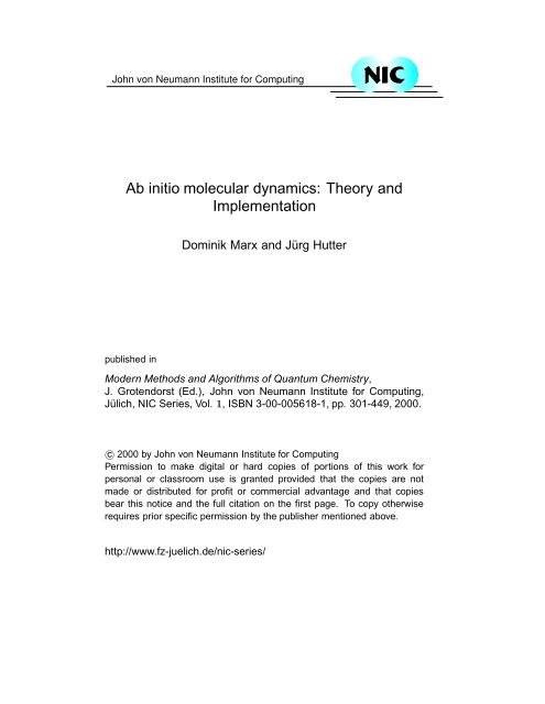
2500Number200015001000CP PRL 1985AIMD50001970 1980 1990 2000Year nFigure 1. Publication and citation analysis. Squares: number of publications which appearedup to the year n that contain the keyword “ab initio molecular dynamics” (or synonyma suchas “first principles MD”, “Car–Parrinello simulations” etc.) in title, abstract or keyword list.Circles: number of publications which appeared up to the year n that cite the 1985 paper byCar and Parrinello 108 (including misspellings of the bibliographic reference). Self–citations andself–papers are excluded, i.e. citations of Ref. 108 in their own papers and papers coauthored byR. Car and / or M. Parrinello are not considered in the respective statistics. The analysis is basedon the CAPLUS (“Chemical Abstracts Plus”), INSPEC (“Physics Abstracts”), and SCI (“ScienceCitation Index”) data bases at STN International. Updated statistics from Ref. 405 .standard molecular dynamics. Another appealing feature of standard moleculardynamics is less evident, namely the “experimental aspect of playing with the potential”.Thus, tracing back the properties of a given system to a simple physicalpicture or mechanism is much harder in ab initio molecular dynamics. The brightside is that new phenomena, which were not forseen before starting the simulation,can simply happen if necessary. This gives ab initio molecular dynamics a trulypredictive power.Ab initio molecular dynamics can also be viewed from another corner, namelyfrom the field of classical trajectory calculations 649,541 . In this approach, whichhas its origin in gas phase molecular dynamics, a global potential energy surfaceis constructed in a first step either empirically or based on electronic structurecalculations. In a second step, the dynamical evolution of the nuclei is generatedby using classical mechanics, quantum mechanics or semi / quasiclassical approximationsof various sorts. In the case of using classical mechanics to describe thedynamics – the focus of the present overview – the limiting step for large systems is3

ut all three ab initio approaches to molecular dynamics are contrasted and partlycompared. The important issue of how to obtain the correct forces in these schemesis discussed in some depth. The most popular electronic structure theories implementedwithin ab initio molecular dynamics, density functional theory in the firstplace but also the Hartree–Fock approach, are sketched. Some attention is alsogiven to another important ingredient in ab initio molecular dynamics, the choiceof the basis set.Concerning the depth, the focus of the present discussion is clearly the implementationof both the basic Car–Parrinello and Born–Oppenheimer moleculardynamics schemes in the CPMD package 142 . The electronic structure approachin CPMD is Hohenberg–Kohn–Sham density functional theory within a plane wave/ pseudopotential implementation and the Generalized Gradient Approximation.The formulae for energies, forces, stress, pseudopotentials, boundary conditions,optimization procedures, parallelization etc. are given for this particular choice tosolve the electronic structure problem. One should, however, keep in mind thata variety of other powerful ab initio molecular dynamics codes are available (forinstance CASTEP 116 , CP-PAW 143 , fhi98md 189 , NWChem 446 , VASP 663 ) which arepartly based on very similar techniques. The classic Car–Parrinello approach 108is then extended to other ensembles than the microcanonical one, other electronicstates than the ground state, and to a fully quantum–mechanical representation ofthe nuclei. Finally, the wealth of problems that can be addressed using ab initiomolecular dynamics is briefly sketched at the end, which also serves implicitly asthe “Summary and Conclusions” section.2 Basic Techniques: Theory2.1 Deriving Classical Molecular DynamicsThe starting point of the following discussion is non–relativistic quantum mechanicsas formalized via the time–dependent Schrödinger equationi∂∂t Φ({r i}, {R I }; t) = HΦ({r i }, {R I }; t) (1)in its position representation in conjunction with the standard HamiltonianH = − ∑ I22M I∇ 2 I − ∑ i2∇ 2 i + ∑ 2m e |r i − r j | − ∑ e 2 Z I|R I − r i | + ∑ e 2 Z I Z J|R I − R J |i

The goal of this section is to derive classical molecular dynamics 12,270,217starting from Schrödinger’s wave equation and following the elegant route ofTully 650,651 . To this end, the nuclear and electronic contributions to the totalwavefunction Φ({r i }, {R I }; t), which depends on both the nuclear and electroniccoordinates, have to be separated. The simplest possible form is a product ansatz[ ∫ i t]Φ({r i }, {R I }; t) ≈ Ψ({r i }; t) χ({R I }; t) exp dt ′ Ẽ e (t ′ ) , (3)t 0where the nuclear and electronic wavefunctions are separately normalized to unityat every instant of time, i.e. 〈χ; t|χ; t〉 = 1 and 〈Ψ; t|Ψ; t〉 = 1, respectively. Inaddition, a convenient phase factor∫Ẽ e = drdR Ψ ⋆ ({r i }; t) χ ⋆ ({R I }; t) H e Ψ({r i }; t) χ({R I }; t) (4)was introduced at this stage such that the final equations will look nice; ∫ drdRrefers to the integration over all i = 1, . . . and I = 1, . . . variables {r i } and {R I },respectively. It is mentioned in passing that this approximation is called a one–determinant or single–configuration ansatz for the total wavefunction, which at theend must lead to a mean–field description of the coupled dynamics. Note also thatthis product ansatz (excluding the phase factor) differs from the Born–Oppenheimeransatz 340,350 for separating the fast and slow variablesΦ BO ({r i }, {R I }; t) =∞∑˜Ψ k ({r i }, {R I })˜χ k ({R I }; t) (5)k=0even in its one–determinant limit, where only a single electronic state k (evaluatedfor the nuclear configuration {R I }) is included in the expansion.Inserting the separation ansatz Eq. (3) into Eqs. (1)–(2) yields (after multiplyingfrom the left by 〈Ψ| and 〈χ| and imposing energy conservation d 〈H〉 /dt ≡ 0) thefollowing relationsi ∂Ψ∂t = − ∑ ii ∂χ∂t = − ∑ I2{∫∇ 22miΨ +e2{∫∇ 22MIχ +I}dR χ ⋆ ({R I }; t)V n−e ({r i }, {R I })χ({R I }; t) Ψ (6)}dr Ψ ⋆ ({r i }; t)H e ({r i }, {R I })Ψ({r i }; t) χ . (7)This set of coupled equations defines the basis of the time–dependent self–consistentfield (TDSCF) method introduced as early as 1930 by Dirac 162 , see also Ref. 158 .Both electrons and nuclei move quantum–mechanically in time–dependent effectivepotentials (or self–consistently obtained average fields) obtained from appropriateaverages (quantum mechanical expectation values 〈. . . 〉) over the other class ofdegrees of freedom (by using the nuclear and electronic wavefunctions, respectively).Thus, the single–determinant ansatz Eq. (3) produces, as already anticipated, amean–field description of the coupled nuclear–electronic quantum dynamics. Thisis the price to pay for the simplest possible separation of electronic and nuclearvariables.6

The next step in the derivation of classical molecular dynamics is the task toapproximate the nuclei as classical point particles. How can this be achieved in theframework of the TDSCF approach, given one quantum–mechanical wave equationdescribing all nuclei? A well–known route to extract classical mechanics fromquantum mechanics in general starts with rewriting the corresponding wavefunctionχ({R I }; t) = A({R I }; t) exp [iS({R I }; t)/ ] (8)in terms of an amplitude factor A and a phase S which are both considered to bereal and A > 0 in this polar representation, see for instance Refs. 163,425,535 . Aftertransforming the nuclear wavefunction in Eq. (7) accordingly and after separatingthe real and imaginary parts, the TDSCF equation for the nuclei∂S∂t + ∑ I∂A∂t + ∑ I∫1(∇ I S) 2 +2M I1M I(∇ I A) (∇ I S) + ∑ Idr Ψ ⋆ H e Ψ = 2 ∑ I1 ∇ 2 I A2M I A(9)12M IA ( ∇ 2 I S) = 0 (10)is (exactly) re–expressed in terms of the new variables A and S. This so–called“quantum fluid dynamical representation” Eqs. (9)–(10) can actually be used tosolve the time–dependent Schrödinger equation 160 . The relation for A, Eq. (10),can be rewritten as a continuity equation 163,425,535 with the help of the identificationof the nuclear density |χ| 2 ≡ A 2 as directly obtained from the definitionEq. (8). This continuity equation is independent of and ensures locally the conservationof the particle probability |χ| 2 associated to the nuclei in the presence ofa flux.More important for the present purpose is a more detailed discussion of therelation for S, Eq. (9). This equation contains one term that depends on , acontribution that vanishes if the classical limit∂S∂t + ∑ I12M I(∇ I S) 2 +∫dr Ψ ⋆ H e Ψ = 0 (11)is taken as → 0; an expansion in terms of would lead to a hierarchy of semiclassicalmethods 425,259 . The resulting equation is now isomorphic to equations ofmotion in the Hamilton–Jacobi formulation 244,540∂S∂t + H ({R I}, {∇ I S}) = 0 (12)of classical mechanics with the classical Hamilton functionH({R I }, {P I }) = T({P I }) + V ({R I }) (13)defined in terms of (generalized) coordinates {R I } and their conjugate momenta{P I }. With the help of the connecting transformationP I ≡ ∇ I S (14)7

¡the Newtonian equation of motion Ṗ I = −∇ I V ({R I }) corresponding to Eq. (11)∫dP I= −∇ I dr Ψ ⋆ H e Ψ ordt∫M I ¨R I (t) = −∇ I dr Ψ ⋆ H e Ψ (15)= −∇ I V Ee ({R I(t)}) (16)can be read off. Thus, the nuclei move according to classical mechanics in aneffective potential Ve E due to the electrons. This potential is a function of only thenuclear positions at time t as a result of averaging H e over the electronic degreesof freedom, i.e. computing its quantum expectation value 〈Ψ|H e |Ψ〉, while keepingthe nuclear positions fixed at their instantaneous values {R I (t)}.However, the nuclear wavefunction still occurs in the TDSCF equation for theelectronic degrees of freedom and has to be replaced by the positions of the nuclei forconsistency. In this case the classical reduction can be achieved simply by replacingthe nuclear density |χ({R I }; t)| 2 in Eq. (6) in the limit → 0 by a product of deltafunctions ∏ I δ(R I − R I (t)) centered at the instantaneous positions {R I (t)} of theclassical nuclei as given by Eq. (15). This yields e.g. for the position operator∫dR χ ⋆ →0({R I }; t) R I χ({R I }; t) −→ R I (t) (17)the required expectation value. This classical limit leads to a time–dependent waveequation for the electronsi ∂Ψ∂t = − ∑ 2∇ 2 i2m Ψ + V n−e({r i }, {R I (t)})Ψi e= H e ({r i }, {R I (t)}) Ψ({r i }, {R I }; t) (18)which evolve self–consistently as the classical nuclei are propagated via Eq. (15).Note that now H e and thus Ψ depend parametrically on the classical nuclear positions{R I (t)} at time t through V n−e ({r i }, {R I (t)}). This means that feedbackbetween the classical and quantum degrees of freedom is incorporated in bothdirections (at variance with the “classical path” or Mott non–SCF approach todynamics 650,651 ).The approach relying on solving Eq. (15) together with Eq. (18) is sometimescalled “Ehrenfest molecular dynamics” in honor of Ehrenfest who was the first toaddress the question a of how Newtonian classical dynamics can be derived fromSchrödinger’s wave equation 174 . In the present case this leads to a hybrid ormixed approach because only the nuclei are forced to behave like classical particles,whereas the electrons are still treated as quantum objects.Although the TDSCF approach underlying Ehrenfest molecular dynamicsclearly is a mean–field theory, transitions between electronic states are includeda The opening statement of Ehrenfest’s famous 1927 paper 174 reads:“Es ist wünschenswert, die folgende Frage möglichst elementar beantworten zu können: WelcherRückblick ergibt sich vom Standpunkt der Quantenmechanik auf die Newtonschen Grundgleichungender klassischen Mechanik?”8

ing numericallyM I ¨R I (t) = −∇ I∫dr Ψ ⋆ H e Ψ= −∇ I 〈Ψ |H e |Ψ〉 (25)= −∇ I 〈H e 〉= −∇ I VeE[i ∂Ψ∂t = − ∑ ]2∇ 2 i2m + V n−e({r i }, {R I (t)}) Ψi e= H e Ψ (26)the coupled set of equations simultaneously. Thereby, the a priori constructionof any type of potential energy surface is avoided from the outset by solving thetime–dependent electronic Schrödinger equation “on–the–fly”. This allows one tocompute the force from ∇ I 〈H e 〉 for each configuration {R I (t)} generated by moleculardynamics; see Sect. 2.5 for the issue of using the so–called “Hellmann–Feynmanforces” instead.The corresponding equations of motion in terms of the adiabatic basis Eq. (20)and the time–dependent expansion coefficients Eq. (19) read 650,651M I ¨R I (t) = − ∑ |c k (t)| 2 ∇ I E k − ∑kk,l∑i ċ k (t) = c k (t)E k − iI,lc ⋆ k c l (E k − E l )d klI (27)c l (t)Ṙ I d klI , (28)where the coupling terms are given byd klI ({R I (t)}) =∫dr Ψ ⋆ k∇ I Ψ l (29)with the property d kkI≡ 0. The Ehrenfest approach is thus seen to include rigorouslynon–adiabatic transitions between different electronic states Ψ k and Ψ l withinthe framework of classical nuclear motion and the mean–field (TDSCF) approximationto the electronic structure, see e.g. Refs. 650,651 for reviews and for instanceRef. 532 for an implementation in terms of time–dependent density functional theory.The restriction to one electronic state in the expansion Eq. (19), which is inmost cases the ground state Ψ 0 , leads toM I ¨R I (t) = −∇ I 〈Ψ 0 |H e | Ψ 0 〉 (30)i ∂Ψ 0∂t= H e Ψ 0 (31)as a special case of Eqs. (25)–(26); note that H e is time–dependent via the nuclearcoordinates {R I (t)}. A point worth mentioning here is that the propagation of thewavefunction is unitary, i.e. the wavefunction preserves its norm and the set oforbitals used to build up the wavefunction will stay orthonormal, see Sect. 2.6.11

Ehrenfest molecular dynamics is certainly the oldest approach to “on–the–fly”molecular dynamics and is typically used for collision– and scattering–type problems154,649,426,532 . However, it was never in widespread use for systems with manyactive degrees of freedom typical for condensed matter problems for reasons thatwill be outlined in Sec. 2.6 (although a few exceptions exist 553,34,203,617 but herethe number of explicitly treated electrons is fairly limited with the exception ofRef. 617 ).2.3 Born–Oppenheimer Molecular DynamicsAn alternative approach to include the electronic structure in molecular dynamicssimulations consists in straightforwardly solving the static electronic structure problemin each molecular dynamics step given the set of fixed nuclear positions at thatinstance of time. Thus, the electronic structure part is reduced to solving a time–independent quantum problem, e.g. by solving the time–independent Schrödingerequation, concurrently to propagating the nuclei via classical molecular dynamics.Thus, the time–dependence of the electronic structure is a consequence of nuclearmotion, and not intrinsic as in Ehrenfest molecular dynamics. The resulting Born–Oppenheimer molecular dynamics method is defined byM I ¨R I (t) = −∇ I min {〈Ψ 0 |H e | Ψ 0 〉}Ψ 0(32)E 0 Ψ 0 = H e Ψ 0 (33)for the electronic ground state. A deep difference with respect to Ehrenfest dynamicsconcerning the nuclear equation of motion is that the minimum of 〈H e 〉has to be reached in each Born–Oppenheimer molecular dynamics step accordingto Eq. (32). In Ehrenfest dynamics, on the other hand, a wavefunction that minimized〈H e 〉 initially will also stay in its respective minimum as the nuclei moveaccording to Eq. (30)!A natural and straightforward extension 281 of ground–state Born–Oppenheimerdynamics is to apply the same scheme to any excited electronic state Ψ k withoutconsidering any interferences. In particular, this means that also the “diagonalcorrection terms” 340∫DI kk ({R I(t)}) = − dr Ψ ⋆ k ∇2 I Ψ k (34)are always neglected; the inclusion of such terms is discussed for instance inRefs. 650,651 . These terms renormalize the Born–Oppenheimer or “clamped nuclei”potential energy surface E k of a given state Ψ k (which might also be theground state Ψ 0 ) and lead to the so–called “adiabatic potential energy surface”of that state 340 . Whence, Born–Oppenheimer molecular dynamics should not becalled “adiabatic molecular dynamics”, as is sometime done.It is useful for the sake of later reference to formulate the Born–Oppenheimerequations of motion for the special case of effective one–particle Hamiltonians. Thismight be the Hartree–Fock approximation defined to be the variational minimumof the energy expectation value 〈Ψ 0 |H e | Ψ 0 〉 given a single Slater determinant Ψ 0 =det{ψ i } subject to the constraint that the one–particle orbitals ψ i are orthonormal12

〈ψ i |ψ j 〉 = δ ij . The corresponding constraint minimization of the total energy withrespect to the orbitalsmin {〈Ψ 0 |H e |Ψ 0 〉} ∣(35){ψ i}can be cast into Lagrange’s formalism∣{〈ψi|ψ j 〉=δ ij }L = − 〈Ψ 0 |H e | Ψ 0 〉 + ∑ i,jΛ ij (〈ψ i |ψ j 〉 − δ ij ) (36)where Λ ij are the associated Lagrangian multipliers. Unconstrained variation ofthis Lagrangian with respect to the orbitalsδLδψ ⋆ ileads to the well–known Hartree–Fock equations!= 0 (37)H HFe ψ i = ∑ jΛ ij ψ j (38)as derived in standard text books 604,418 ; the diagonal canonical form H HFe ψ i = ɛ i ψ iis obtained after a unitary transformation and H HFe denotes the effective one–particle Hamiltonian, see Sect. 2.7 for more details. The equations of motioncorresponding to Eqs. (32)–(33) read{〈 ∣ 〉}M I ¨R I (t) = −∇ I min Ψ0 ∣H HF∣ e Ψ0 (39){ψ i}0 = −H HFe ψ i + ∑ jΛ ij ψ j (40)for the Hartree–Fock case. A similar set of equations is obtained if Hohenberg–Kohn–Sham density functional theory 458,168 is used, where H HFe has to be replacedby the Kohn–Sham effective one–particle Hamiltonian HeKS , see Sect. 2.7 for moredetails. Instead of diagonalizing the one–particle Hamiltonian an alternative butequivalent approach consists in directly performing the constraint minimizationaccording to Eq. (35) via nonlinear optimization techniques.Early applications of Born–Oppenheimer molecular dynamics were performedin the framework of a semiempirical approximation to the electronic structure problem669,671 . But only a few years later an ab initio approach was implemented withinthe Hartree–Fock approximation 365 . Born–Oppenheimer dynamics started to becomepopular in the early nineties with the availability of more efficient electronicstructure codes in conjunction with sufficient computer power to solve “interestingproblems”, see for instance the compilation of such studies in Table 1 in a recentoverview article 82 .Undoubtedly, the breakthrough of Hohenberg–Kohn–Sham density functionaltheory in the realm of chemistry – which took place around the same time – alsohelped a lot by greatly improving the “price / performance ratio” of the electronicstructure part, see e.g. Refs. 694,590 . A third and possibly the crucial reason thatboosted the field of ab initio molecular dynamics was the pioneering introduction of13

the Car–Parrinello approach 108 , see also Fig. 1. This technique opened novel avenuesto treat large–scale problems via ab initio molecular dynamics and catalyzedthe entire field by making “interesting calculations” possible, see also the closingsection on applications.2.4 Car–Parrinello Molecular Dynamics2.4.1 MotivationA non–obvious approach to cut down the computational expenses of molecular dynamicswhich includes the electrons in a single state was proposed by Car andParrinello in 1985 108 . In retrospect it can be considered to combine the advantagesof both Ehrenfest and Born–Oppenheimer molecular dynamics. In Ehrenfestdynamics the time scale and thus the time step to integrate Eqs. (30) and (31)simultaneously is dictated by the intrinsic dynamics of the electrons. Since electronicmotion is much faster than nuclear motion, the largest possible time stepis that which allows to integrate the electronic equations of motion. Contraryto that, there is no electron dynamics whatsoever involved in solving the Born–Oppenheimer Eqs. (32)–(33), i.e. they can be integrated on the time scale givenby nuclear motion. However, this means that the electronic structure problemhas to be solved self–consistently at each molecular dynamics step, whereas this isavoided in Ehrenfest dynamics due to the possibility to propagate the wavefunctionby applying the Hamiltonian to an initial wavefunction (obtained e.g. by oneself–consistent diagonalization).From an algorithmic point of view the main task achieved in ground–stateEhrenfest dynamics is simply to keep the wavefunction automatically minimizedas the nuclei are propagated. This, however, might be achieved – in principle – byanother sort of deterministic dynamics than first–order Schrödinger dynamics. Insummary, the “Best of all Worlds Method” should (i) integrate the equations ofmotion on the (long) time scale set by the nuclear motion but nevertheless (ii) takeintrinsically advantage of the smooth time–evolution of the dynamically evolvingelectronic subsystem as much as possible. The second point allows to circumventexplicit diagonalization or minimization to solve the electronic structure problemfor the next molecular dynamics step. Car–Parrinello molecular dynamics is an efficientmethod to satisfy requirement (ii) in a numerically stable fashion and makesan acceptable compromise concerning the length of the time step (i).2.4.2 Car–Parrinello Lagrangian and Equations of MotionThe basic idea of the Car–Parrinello approach can be viewed to exploit thequantum–mechanical adiabatic time–scale separation of fast electronic and slownuclear motion by transforming that into classical–mechanical adiabatic energy–scale separation in the framework of dynamical systems theory. In order to achievethis goal the two–component quantum / classical problem is mapped onto a two–component purely classical problem with two separate energy scales at the expenseof loosing the explicit time–dependence of the quantum subsystem dynamics. Furthermore,the central quantity, the energy of the electronic subsystem 〈Ψ 0 |H e |Ψ 0 〉14

evaluated with some wavefunction Ψ 0 , is certainly a function of the nuclear positions{R I }. But at the same time it can be considered to be a functional of thewavefunction Ψ 0 and thus of a set of one–particle orbitals {ψ i } (or in general ofother functions such as two–particle geminals) used to build up this wavefunction(being for instance a Slater determinant Ψ 0 = det{ψ i } or a combination thereof).Now, in classical mechanics the force on the nuclei is obtained from the derivativeof a Lagrangian with respect to the nuclear positions. This suggests that afunctional derivative with respect to the orbitals, which are interpreted as classicalfields, might yield the force on the orbitals, given a suitable Lagrangian. In addition,possible constraints within the set of orbitals have to be imposed, such as e.g.orthonormality (or generalized orthonormality conditions that include an overlapmatrix).Car and Parrinello postulated the following class of Lagrangians 108L CP = ∑ 12 MIṘ2 I + ∑ 1〈 ∣ 〉 ∣∣2 µ i ˙ψ i ˙ψ i − 〈Ψ 0 |H e |Ψ 0 〉} {{ }Ii} {{ } potential energykinetic energy+ constraints} {{ }(41)orthonormalityto serve this purpose. The corresponding Newtonian equations of motion are obtainedfrom the associated Euler–Lagrange equationsd ∂L= ∂Ldt ∂Ṙ I∂R I(42)d δLdt δ ˙ψ= δLi⋆ δψi⋆ (43)like in classical mechanics, but here for both the nuclear positions and the orbitals;note ψ ⋆ i = 〈ψ i| and that the constraints are holonomic 244 . Following this route ofideas, generic Car–Parrinello equations of motion are found to be of the formM I ¨R I (t) = −∂ 〈Ψ 0 |H e |Ψ 0 〉 +∂ {constraints} (44)∂R I ∂R Iµ i ¨ψi (t) = − δδψ ⋆ i〈Ψ 0 |H e |Ψ 0 〉 + δδψ ⋆ i{constraints} (45)where µ i (= µ) are the “fictitious masses” or inertia parameters assigned to theorbital degrees of freedom; the units of the mass parameter µ are energy times asquared time for reasons of dimensionality. Note that the constraints within thetotal wavefunction lead to “constraint forces” in the equations of motion. Note alsothat these constraintsconstraints = constraints ({ψ i }, {R I }) (46)might be a function of both the set of orbitals {ψ i } and the nuclear positions {R I }.These dependencies have to be taken into account properly in deriving the Car–Parrinello equations following from Eq. (41) using Eqs. (42)–(43), see Sect. 2.5 fora general discussion and see e.g. Ref. 351 for a case with an additional dependenceof the wavefunction constraint on nuclear positions.15

According to the Car–Parrinello equations of motion, the nuclei evolve in timeat a certain (instantaneous) physical temperature ∝ ∑ I MIṘ2 I , whereas a “fictitioustemperature” ∝ ∑ i µ i〈 ˙ψ i | ˙ψ i 〉 is associated to the electronic degrees offreedom. In this terminology, “low electronic temperature” or “cold electrons”means that the electronic subsystem is close to its instantaneous minimum energymin {ψi}〈Ψ 0 |H e |Ψ 0 〉, i.e. close to the exact Born–Oppenheimer surface. Thus, aground–state wavefunction optimized for the initial configuration of the nuclei willstay close to its ground state also during time evolution if it is kept at a sufficientlylow temperature.The remaining task is to separate in practice nuclear and electronic motion suchthat the fast electronic subsystem stays cold also for long times but still followsthe slow nuclear motion adiabatically (or instantaneously). Simultaneously, thenuclei are nevertheless kept at a much higher temperature. This can be achievedin nonlinear classical dynamics via decoupling of the two subsystems and (quasi–)adiabatic time evolution. This is possible if the power spectra stemming fromboth dynamics do not have substantial overlap in the frequency domain so thatenergy transfer from the “hot nuclei” to the “cold electrons” becomes practicallyimpossible on the relevant time scales. This amounts in other words to imposing andmaintaining a metastability condition in a complex dynamical system for sufficientlylong times. How and to which extend this is possible in practice was investigated indetail in an important investigation based on well–controlled model systems 467,468(see also Sects. 3.2 and 3.3 in Ref. 513 ), with more mathematical rigor in Ref. 86 ,and in terms of a generalization to a second level of adiabaticity in Ref. 411 .2.4.3 Why Does the Car–Parrinello Method Work ?In order to shed light on the title question, the dynamics generated by the Car–Parrinello Lagrangian Eq. (41) is analyzed 467 in more detail invoking a “classicaldynamics perspective” of a simple model system (eight silicon atoms forming aperiodic diamond lattice, local density approximation to density functional theory,normconserving pseudopotentials for core electrons, plane wave basis for valenceorbitals, 0.3 fs time step with µ = 300 a.u., in total 20 000 time steps or 6.3 ps),for full details see Ref. 467 ); a concise presentation of similar ideas can be foundin Ref. 110 . For this system the vibrational density of states or power spectrumof the electronic degrees of freedom, i.e. the Fourier transform of the statisticallyaveraged velocity autocorrelation function of the classical fields∫ ∞f(ω) = dt cos(ωt) ∑ 〈 ˙ψ i ; t ∣ ˙ψ〉i ; 0(47)0iis compared to the highest–frequency phonon mode ωnmax of the nuclear subsystemin Fig. 2. From this figure it is evident that for the chosen parameters the nuclearand electronic subsystems are dynamically separated: their power spectra do notoverlap so that energy transfer from the hot to the cold subsystem is expected tobe prohibitively slow, see Sect. 3.3 in Ref. 513 for a similar argument.This is indeed the case as can be verified in Fig. 3 where the conserved energyE cons , physical total energy E phys , electronic energy V e , and fictitious kinetic energy16

Figure 3. Various energies Eqs. (48)–(51) for a model system propagatedvia Car–Parrinellomoleculardynamics for at short (up to 300 fs), intermediate, and long times (up to 6.3 ps); for furtherdetails see text. Adapted from Ref. 467 .for the stability of the Car–Parrinello dynamics, vide infra. But already the visiblevariations are three orders of magnitude smaller than the physically meaningful oscillationsof V e . As a result, E phys defined as E cons − T e or equivalently as the sumof the nuclear kinetic energy and the electronic total energy (which serves as thepotential energy for the nuclei) is essentially constant on the relevant energy andtime scales. Thus, it behaves approximately like the strictly conserved total energyin classical molecular dynamics (with only nuclei as dynamical degrees of freedom)or in Born–Oppenheimer molecular dynamics (with fully optimized electronic degreesof freedom) and is therefore often denoted as the “physical total energy”.This implies that the resulting physically significant dynamics of the nuclei yieldsan excellent approximation to microcanonical dynamics (and assuming ergodicityto the microcanonical ensemble). Note that a different explanation was advocatedin Ref. 470 (see also Ref. 472 , in particular Sect. VIII.B and C), which was howeverrevised in Ref. 110 . A discussion similar in spirit to the one outlined here 467 isprovided in Ref. 513 , see in particular Sect. 3.2 and 3.3.Given the adiabatic separation and the stability of the propagation, the centralquestion remains if the forces acting on the nuclei are actually the “correct” onesin Car–Parrinello molecular dynamics. As a reference serve the forces obtainedfrom full self–consistent minimizations of the electronic energy min {ψi}〈Ψ 0 |H e |Ψ 0 〉at each time step, i.e. Born–Oppenheimer molecular dynamics with extremely wellconverged wavefunctions. This is indeed the case as demonstrated in Fig. 4(a):the physically meaningful dynamics of the x–component of the force acting on onesilicon atom in the model system obtained from stable Car–Parrinello fictitiousdynamics propagation of the electrons and from iterative minimizations of the electronicenergy are extremely close.Better resolution of one oscillation period in (b) reveals that the gross deviationsare also oscillatory but that they are four orders of magnitudes smaller than18

Figure 4. (a) Comparison of the x–component of the force acting on one atom of a model systemobtained from Car–Parrinello (solid line) and well–converged Born–Oppenheimer (dots) moleculardynamics. (b) Enlarged view of the difference between Car–Parrinello and Born–Oppenheimerforces; for further details see text. Adapted from Ref. 467 .the physical variations of the force resolved in Fig. 4(a). These correspond to the“large–amplitude” oscillations of T e visible in Fig. 3 due to the drag of the nucleiexerted on the quasi–adiabatically following electrons having a finite dynamicalmass µ. Note that the inertia of the electrons also dampens artificially the nuclearmotion (typically on a few–percent scale, see Sect. V.C.2 in Ref. 75 for an analysisand a renormalization correction of M I ) but decreases as the fictitious massapproaches the adiabatic limit µ → 0. Superimposed on the gross variation in (b)are again high–frequency bound oscillatory small–amplitude fluctuations like for T e .They lead on physically relevant time scales (i.e. those visible in Fig. 4(a)) to “averagedforces” that are very close to the exact ground–state Born–Oppenheimerforces. This feature is an important ingredient in the derivation of adiabatic dynamics467,411 .In conclusion, the Car–Parrinello force can be said to deviate at most instants oftime from the exact Born–Oppenheimer force. However, this does not disturb thephysical time evolution due to (i) the smallness and boundedness of this differenceand (ii) the intrinsic averaging effect of small–amplitude high–frequency oscillationswithin a few molecular dynamics time steps, i.e. on the sub–femtosecond time scalewhich is irrelevant for nuclear dynamics.2.4.4 How to Control Adiabaticity ?An important question is under which circumstances the adiabatic separation canbe achieved, and how it can be controlled. A simple harmonic analysis of thefrequency spectrum of the orbital classical fields close to the minimum defining theground state yields 467 ( ) 1/2 2(ɛi − ɛ j )ω ij =, (52)µ19

where ɛ j and ɛ i are the eigenvalues of occupied and unoccupied orbitals, respectively;see Eq. (26) in Ref. 467 for the case where both orbitals are occupied ones.It can be seen from Fig. 2 that the harmonic approximation works faithfully ascompared to the exact spectrum; see Ref. 471 and Sect. IV.A in Ref. 472 for a moregeneral analysis of the associated equations of motion. Since this is in particulartrue for the lowest frequency ωemin , the handy analytic estimate for the lowestpossible electronic frequencyω mine∝(Egapµ) 1/2, (53)shows that this frequency increases like the square root of the electronic energydifference E gap between the lowest unoccupied and the highest occupied orbital.On the other hand it increases similarly for a decreasing fictitious mass parameterµ.ω maxnIn order to guarantee the adiabatic separation, the frequency difference ωemin −should be large, see Sect. 3.3 in Ref. 513 for a similar argument. But boththe highest phonon frequency ωnmax and the energy gap E gap are quantities that adictated by the physics of the system. Whence, the only parameter in our handsto control adiabatic separation is the fictitious mass, which is therefore also called“adiabaticity parameter”. However, decreasing µ not only shifts the electronicspectrum upwards on the frequency scale, but also stretches the entire frequencyspectrum according to Eq. (52). This leads to an increase of the maximum frequencyaccording toω maxe∝(Ecutµ) 1/2, (54)where E cut is the largest kinetic energy in an expansion of the wavefunction interms of a plane wave basis set, see Sect. 3.1.3.At this place a limitation to decrease µ arbitrarily kicks in due to the maximumlength of the molecular dynamics time step ∆t max that can be used. The time stepis inversely proportional to the highest frequency in the system, which is ωemax andthus the relation( ) 1/2 µ∆t max ∝(55)E cutgoverns the largest time step that is possible. As a consequence, Car–Parrinellosimulators have to find their way between Scylla and Charybdis and have to makea compromise on the control parameter µ; typical values for large–gap systems areµ = 500–1500 a.u. together with a time step of about 5–10 a.u. (0.12–0.24 fs).Recently, an algorithm was devised that optimizes µ during a particular simulationgiven a fixed accuracy criterion 87 . Note that a poor man’s way to keep the timestep large and still increase µ in order to satisfy adiabaticity is to choose heaviernuclear masses. That depresses the largest phonon or vibrational frequency ωnmaxof the nuclei (at the cost of renormalizing all dynamical quantities in the sense ofclassical isotope effects).20

Up to this point the entire discussion of the stability and adiabaticity issueswas based on model systems, approximate and mostly qualitative in nature. Butrecently it was actually proven 86 that the deviation or the absolute error ∆ µ of theCar–Parrinello trajectory relative to the trajectory obtained on the exact Born–Oppenheimer potential energy surface is controlled by µ:Theorem 1 iv.): There are constants C > 0 and µ ⋆ > 0 such that∆ µ = ∣ ∣ R µ (t) − R 0 (t) ∣ ∣ +∣ ∣|ψ µ ; t〉 − ∣ ∣ ψ 0 ; t 〉∣ ∣ ≤ Cµ1/2, 0 ≤ t ≤ T (56)and the fictitious kinetic energy satisfiesT e = 1 〈 2 µ ˙ψ µ ; t ∣ ˙ψ〉µ ; t ≤ Cµ , 0 ≤ t ≤ T (57)for all values of the parameter µ satisfying 0 < µ ≤ µ ⋆ , where up to time T > 0there exists a unique nuclear trajectory on the exact Born–Oppenheimer surfacewith ωemin > 0 for 0 ≤ t ≤ T, i.e. there is “always” a finite electronic excitationgap. Here, the superscript µ or 0 indicates that the trajectory was obtained viaCar–Parrinello molecular dynamics using a finite mass µ or via dynamics on theexact Born–Oppenheimer surface, respectively. Note that not only the nucleartrajectory is shown to be close to the correct one, but also the wavefunction isproven to stay close to the fully converged one up to time T. Furthermore, itwas also investigated what happens if the initial wavefunction at t = 0 is not theminimum of the electronic energy 〈H e 〉 but trapped in an excited state. In this caseit is found that the propagated wavefunction will keep on oscillating at t > 0 alsofor µ → 0 and not even time averages converge to any of the eigenstates. Note thatthis does not preclude Car–Parrinello molecular dynamics in excited states, which ispossible given a properly “minimizable” expression for the electronic energy, see e.g.Refs. 281,214 . However, this finding might have crucial implications for electroniclevel–crossing situations.What happens if the electronic gap is very small or even vanishes E gap → 0as is the case for metallic systems? In this limit, all the above–given argumentsbreak down due to the occurrence of zero–frequency electronic modes in the powerspectrum according to Eq. (53), which necessarily overlap with the phonon spectrum.Following an idea of Sprik 583 applied in a classical context it was shownthat the coupling of separate Nosé–Hoover thermostats 12,270,217 to the nuclear andelectronic subsystem can maintain adiabaticity by counterbalancing the energy flowfrom ions to electrons so that the electrons stay “cool” 74 ; see Ref. 204 for a similaridea to restore adiabaticity. Although this method is demonstrated to work inpractice 464 , this ad hoc cure is not entirely satisfactory from both a theoretical andpractical point of view so that the well–controlled Born–Oppenheimer approach isrecommended for strongly metallic systems. An additional advantage for metallicsystems is that the latter is also better suited to sample many k–points (seeSect. 3.1.3), allows easily for fractional occupation numbers 458,168 , and can handleefficiently the so–called charge sloshing problem 472 .21

2.4.5 The Quantum Chemistry ViewpointIn order to understand Car–Parrinello molecular dynamics also from the “quantumchemistry perspective”, it is useful to formulate it for the special case of the Hartree–Fock approximation usingL CP = ∑ 12 MIṘ2 I + ∑ 1〈 ∣ 〉 ∣∣2 µ i ˙ψ i ˙ψ iIi− 〈 〉 ∑Ψ 0 |H HFe |Ψ 0 + Λ ij (〈ψ i |ψ j 〉 − δ ij ) . (58)The resulting equations of motioni,jM I ¨R I (t) = −∇ I〈Ψ0∣ ∣ H HFeµ i ¨ψi (t) = −H HFe ψ i + ∑ j∣ 〉∣Ψ 0(59)Λ ij ψ j (60)are very close to those obtained for Born–Oppenheimer molecular dynamicsEqs. (39)–(40) except for (i) no need to minimize the electronic total energy expressionand (ii) featuring the additional fictitious kinetic energy term associatedto the orbital degrees of freedom. It is suggestive to argue that both sets of equationsbecome identical if the term |µ i ¨ψi (t)| is small at any time t compared to thephysically relevant forces on the right–hand–side of both Eq. (59) and Eq. (60).This term being zero (or small) means that one is at (or close to) the minimum ofthe electronic energy 〈Ψ 0 |H HFe |Ψ 0 〉 since time derivatives of the orbitals {ψ i } canbe considered as variations of Ψ 0 and thus of the expectation value 〈H HFe 〉 itself.In other words, no forces act on the wavefunction if µ i ¨ψi ≡ 0. In conclusion, theCar–Parrinello equations are expected to produce the correct dynamics and thusphysical trajectories in the microcanonical ensemble in this idealized limit. Butif |µ i ¨ψi (t)| is small for all i, this also implies that the associated kinetic energyT e = ∑ i µ i〈 ˙ψ i | ˙ψ i 〉/2 is small, which connects these more qualitative argumentswith the previous discussion 467 .At this stage, it is also interesting to compare the structure of the LagrangianEq. (58) and the Euler–Lagrange equation Eq. (43) for Car–Parrinello dynamics tothe analogues equations (36) and (37), respectively, used to derive “Hartree–Fockstatics”. The former reduce to the latter if the dynamical aspect and the associatedtime evolution is neglected, that is in the limit that the nuclear and electronicmomenta are absent or constant. Thus, the Car–Parrinello ansatz, namely Eq. (41)together with Eqs. (42)–(43), can also be viewed as a prescription to derive a newclass of “dynamical ab initio methods” in very general terms.2.4.6 The Simulated Annealing and Optimization ViewpointsIn the discussion given above, Car–Parrinello molecular dynamics was motivatedby “combining” the positive features of both Ehrenfest and Born–Oppenheimermolecular dynamics as much as possible. Looked at from another side, the Car–Parrinello method can also be considered as an ingenious way to perform globaloptimizations (minimizations) of nonlinear functions, here 〈Ψ 0 |H e |Ψ 0 〉, in a high–dimensional parameter space including complicated constraints. The optimization22

parameters are those used to represent the total wavefunction Ψ 0 in terms of simplerfunctions, for instance expansion coefficients of the orbitals in terms of Gaussiansor plane waves, see e.g. Refs. 583,375,693,608 for applications of the same idea inother fields.Keeping the nuclei frozen for a moment, one could start this optimization procedurefrom a “random wavefunction” which certainly does not minimize the electronicenergy. Thus, its fictitious kinetic energy is high, the electronic degrees offreedom are “hot”. This energy, however, can be extracted from the system bysystematically cooling it to lower and lower temperatures. This can be achievedin an elegant way by adding a non–conservative damping term to the electronicCar–Parrinello equation of motion Eq. (45)µ i ¨ψi (t) = − δδψ ⋆ i〈Ψ 0 |H e |Ψ 0 〉 + δδψ ⋆ i{constraints} − γ e µ i ψ i , (61)where γ e ≥ 0 is a friction constant that governs the rate of energy dissipation 610 ;alternatively, dissipation can be enforced in a discrete fashion by reducing the velocitiesby multiplying them with a constant factor < 1. Note that this deterministicand dynamical method is very similar in spirit to simulated annealing 332 inventedin the framework of the stochastic Monte Carlo approach in the canonical ensemble.If the energy dissipation is done slowly, the wavefunction will find its way down tothe minimum of the energy. At the end, an intricate global optimization has beenperformed!If the nuclei are allowed to move according to Eq. (44) in the presence of anotherdamping term a combined or simultaneous optimization of both electronsand nuclei can be achieved, which amounts to a “global geometry optimization”.This perspective is stressed in more detail in the review Ref. 223 and an implementationof such ideas within the CADPAC quantum chemistry code is described inRef. 692 . This operational mode of Car–Parrinello molecular dynamics is related toother optimization techniques where it is aimed to optimize simultaneously both thestructure of the nuclear skeleton and the electronic structure. This is achieved byconsidering the nuclear coordinates and the expansion coefficients of the orbitals asvariation parameters on the same footing 49,290,608 . But Car–Parrinello moleculardynamics is more than that because even if the nuclei continuously move accordingto Newtonian dynamics at finite temperature an initially optimized wavefunctionwill stay optimal along the nuclear trajectory.2.4.7 The Extended Lagrangian ViewpointThere is still another way to look at the Car–Parrinello method, namely in thelight of so–called “extended Lagrangians” or “extended system dynamics” 14 , seee.g. Refs. 136,12,270,585,217 for introductions. The basic idea is to couple additionaldegrees of freedom to the Lagrangian of interest, thereby “extending” it by increasingthe dimensionality of phase space. These degrees of freedom are treated likeclassical particle coordinates, i.e. they are in general characterized by “positions”,“momenta”, “masses”, “interactions” and a “coupling term” to the particle’s positionsand momenta. In order to distinguish them from the physical degrees offreedom, they are often called “fictitious degrees of freedom”.23

The corresponding equations of motion follow from the Euler–Lagrange equationsand yield a microcanonical ensemble in the extended phase space where theHamiltonian of the extended system is strictly conserved. In other words, theHamiltonian of the physical (sub–) system is no more (strictly) conserved, and theproduced ensemble is no more the microcanonical one. Any extended system dynamicsis constructed such that time–averages taken in that part of phase space thatis associated to the physical degrees of freedom (obtained from a partial trace overthe fictitious degrees of freedom) are physically meaningful. Of course, dynamicsand thermodynamics of the system are affected by adding fictitious degrees of freedom,the classic examples being temperature and pressure control by thermostatsand barostats, see Sect. 4.2.In the case of Car–Parrinello molecular dynamics, the basic Lagrangian forNewtonian dynamics of the nuclei is actually extended by classical fields {ψ i (r)},i.e. functions instead of coordinates, which represent the quantum wavefunction.Thus, vector products or absolute values have to be generalized to scalar productsand norms of the fields. In addition, the “positions” of these fields {ψ i } actuallyhave a physical meaning, contrary to their momenta { ˙ψ i }.2.5 What about Hellmann–Feynman Forces ?An important ingredient in all dynamics methods is the efficient calculation of theforces acting on the nuclei, see Eqs. (30), (32), and (44). The straightforwardnumerical evaluation of the derivativeF I = −∇ I 〈Ψ 0 |H e |Ψ 0 〉 (62)in terms of a finite–difference approximation of the total electronic energy is bothtoo costly and too inaccurate for dynamical simulations. What happens if the gradientsare evaluated analytically? In addition to the derivative of the Hamiltonianitself∇ I 〈Ψ 0 |H e |Ψ 0 〉 = 〈Ψ 0 |∇ I H e |Ψ 0 〉+ 〈∇ I Ψ 0 |H e |Ψ 0 〉 + 〈Ψ 0 |H e |∇ I Ψ 0 〉 (63)there are in general also contributions from variations of the wavefunction ∼ ∇ I Ψ 0 .In general means here that these contributions vanish exactlyF HFTI = − 〈Ψ 0 |∇ I H e |Ψ 0 〉 (64)if the wavefunction is an exact eigenfunction (or stationary state wavefunction) ofthe particular Hamiltonian under consideration. This is the content of the often–cited Hellmann–Feynman Theorem 295,186,368 , which is also valid for many variationalwavefunctions (e.g. the Hartree–Fock wavefunction) provided that completebasis sets are used. If this is not the case, which has to be assumed for numericalcalculations, the additional terms have to be evaluated explicitly.In order to proceed a Slater determinant Ψ 0 = det{ψ i } of one–particle orbitalsψ i , which themselves are expandedψ i = ∑ νc iν f ν (r; {R I }) (65)24

in terms of a linear combination of basis functions {f ν }, is used in conjunction withan effective one–particle Hamiltonian (such as e.g. in Hartree–Fock or Kohn–Shamtheories). The basis functions might depend explicitly on the nuclear positions (inthe case of basis functions with origin such as atom–centered orbitals), whereas theexpansion coefficients always carry an implicit dependence. This means that fromthe outset two sorts of forces are expected∇ I ψ i = ∑ ν(∇ I c iν ) f ν (r; {R I }) + ∑ νc iν (∇ I f ν (r; {R I })) (66)in addition to the Hellmann–Feynman force Eq. (64).Using such a linear expansion Eq. (65), the force contributions stemming fromthe nuclear gradients of the wavefunction in Eq. (63) can be disentangled into twoterms. The first one is called “incomplete–basis–set correction” (IBS) in solid statetheory 49,591,180 and corresponds to the “wavefunction force” 494 or “Pulay force” inquantum chemistry 494,496 . It contains the nuclear gradients of the basis functionsF IBSI= − ∑ iνµ(〈∇I f ν∣ ∣H NSCe− ɛ i∣ ∣fµ〉+〈fν∣ ∣H NSCe − ɛ i∣ ∣ ∇fµ〉)and the (in practice non–self–consistent) effective one–particle Hamiltonian 49,591 .The second term leads to the so–called “non–self–consistency correction” (NSC) ofthe force 49,591F NSCI∫= −(67)dr (∇ I n) ( V SCF − V NSC) (68)and is governed by the difference between the self–consistent (“exact”) potential orfield V SCF and its non–self–consistent (or approximate) counterpart V NSC associatedto H NSCe ; n(r) is the charge density. In summary, the total force needed in abinitio molecular dynamics simulationsF I = F HFTI+ F IBSI+ F NSCI (69)comprises in general three qualitatively different terms; see the tutorial articleRef. 180 for a further discussion of core vs. valence states and the effect of pseudopotentials.Assuming that self–consistency is exactly satisfied (which is never goingvanishes and H SCFe has to. The Pulay contribution vanishes in the limit of using ato be the case in numerical calculations), the force F NSCIbe used to evaluate F IBSIcomplete basis set (which is also not possible to achieve in actual calculations).The most obvious simplification arises if the wavefunction is expanded in termsof originless basis functions such as plane waves, see Eq. (100). In this case the Pulayforce vanishes exactly, which applies of course to all ab initio molecular dynamicsschemes (i.e. Ehrenfest, Born–Oppenheimer, and Car–Parrinello) using that particularbasis set. This statement is true for calculations where the number of planewaves is fixed. If the number of plane waves changes, such as in (constant pressure)calculations with varying cell volume / shape where the energy cutoff is strictlyfixed instead, Pulay stress contributions crop up 219,245,660,211,202 , see Sect. 4.2. Ifbasis sets with origin are used instead of plane waves Pulay forces arise always andhave to be included explicitely in force calculations, see e.g. Refs. 75,370,371 for suchmethods. Another interesting simplification of the same origin is noted in passing:25

there is no basis set superposition error (BSSE) 88 in plane wave–based electronicstructure calculations.A non–obvious and more delicate term in the context of ab initio moleculardynamics is the one stemming from non–self–consistency Eq. (68). This term vanishesonly if the wavefunction Ψ 0 is an eigenfunction of the Hamiltonian within thesubspace spanned by the finite basis set used. This demands less than the Hellmann–Feynman theorem where Ψ 0 has to be an exact eigenfunction of the Hamiltonianand a complete basis set has to be used in turn. In terms of electronic structurecalculations complete self–consistency (within a given incomplete basis set) has tobe reached in order that F NSCI vanishes. Thus, in numerical calculations the NSCterm can be made arbitrarily small by optimizing the effective Hamiltonian and bydetermining its eigenfunctions to very high accuracy, but it can never be suppressedcompletely.The crucial point is, however, that in Car–Parrinello as well as in Ehrenfestmolecular dynamics it is not the minimized expectation value of the electronicHamiltonian, i.e. min Ψ0 {〈Ψ 0 |H e |Ψ 0 〉}, that yields the consistent forces. What ismerely needed is to evaluate the expression 〈Ψ 0 |H e |Ψ 0 〉 with the Hamiltonian andthe associated wavefunction available at a certain time step, compare Eq. (32) toEq. (44) or (30). In other words, it is not required (concerning the present discussionof the contributions to the force!) that the expectation value of the electronicHamiltonian is actually completely minimized for the nuclear configuration at thattime step. Whence, full self–consistency is not required for this purpose in the caseof Car–Parrinello (and Ehrenfest) molecular dynamics. As a consequence, the non–self–consistency correction to the force F NSCIEq. (68) is irrelevant in Car–Parrinello(and Ehrenfest) simulations.In Born–Oppenheimer molecular dynamics, on the other hand, the expectationvalue of the Hamiltonian has to be minimized for each nuclear configuration beforetaking the gradient to obtain the consistent force! In this scheme there is (independentlyfrom the issue of Pulay forces) always the non–vanishing contribution ofthe non–self–consistency force, which is unknown by its very definition (if it wereknow, the problem was solved, see Eq. (68)). It is noted in passing that there areestimation schemes available that correct approximately for this systematic error inBorn–Oppenheimer dynamics and lead to significant time–savings, see e.g. Ref. 344 .Heuristically one could also argue that within Car–Parrinello dynamics the non–vanishing non–self–consistency force is kept under control or counterbalanced bythe non–vanishing “mass times acceleration term” µ i ¨ψi (t) ≈ 0, which is small butnot identical to zero and oscillatory. This is sufficient to keep the propagation stable,whereas µ i ¨ψi (t) ≡ 0, i.e. an extremely tight minimization min Ψ0 {〈Ψ 0 |H e |Ψ 0 〉},is required by its very definition in order to make the Born–Oppenheimer approachstable, compare again Eq. (60) to Eq. (40). Thus, also from this perspective itbecomes clear that the fictitious kinetic energy of the electrons and thus their fictitioustemperature is a measure for the departure from the exact Born–Oppenheimersurface during Car–Parrinello dynamics.Finally, the present discussion shows that nowhere in these force derivations wasmade use of the Hellmann–Feynman theorem as is sometimes stated. Actually, itis known for a long time that this theorem is quite useless for numerical electronic26

structure calculations, see e.g. Refs. 494,49,496 and references therein. Rather itturns out that in the case of Car–Parrinello calculations using a plane wave basisthe resulting relation for the force, namely Eq. (64), looks like the one obtained bysimply invoking the Hellmann–Feynman theorem at the outset.It is interesting to recall that the Hellmann–Feynman theorem as applied to anon–eigenfunction of a Hamiltonian yields only a first–order perturbative estimateof the exact force 295,368 . The same argument applies to ab initio molecular dynamicscalculations where possible force corrections according to Eqs. (67) and (68)are neglected without justification. Furthermore, such simulations can of course notstrictly conserve the total Hamiltonian E cons Eq. (48). Finally, it should be stressedthat possible contributions to the force in the nuclear equation of motion Eq. (44)due to position–dependent wavefunction constraints have to be evaluated followingthe same procedure. This leads to similar “correction terms” to the force, see e.g.Ref. 351 for such a case.2.6 Which Method to Choose ?Presumably the most important question for practical applications is which ab initiomolecular dynamics method is the most efficient in terms of computer time given aspecific problem. An a priori advantage of both the Ehrenfest and Car–Parrinelloschemes over Born–Oppenheimer molecular dynamics is that no diagonalizationof the Hamiltonian (or the equivalent minimization of an energy functional) isnecessary, except at the very first step in order to obtain the initial wavefunction.The difference is, however, that the Ehrenfest time–evolution according tothe time–dependent Schrödinger equation Eq. (26) conforms to a unitary propagation341,366,342 Ψ(t 0 + ∆t) = exp [−iH e (t 0 )∆t/ ]Ψ(t 0 ) (70)Ψ(t 0 + m ∆t) = exp [−iH e (t 0 + (m − 1)∆t) ∆t/ ]× · · ·Ψ(t 0 + t max ) ∆t→0= T exp× exp [−iH e (t 0 + 2∆t) ∆t/ ]× exp [−iH e (t 0 + ∆t) ∆t/ ]× exp [−iH e (t 0 ) ∆t/ ]Ψ(t 0 ) (71)[− i ∫ ]t 0+t maxt 0dt H e (t)Ψ(t 0 ) (72)for infinitesimally short times given by the time step ∆t = t max /m; here T is thetime–ordering operator and H e (t) is the Hamiltonian (which is implicitly time–dependent via the positions {R I (t)}) evaluated at time t using e.g. split operatortechniques 183 . Thus, the wavefunction Ψ will conserve its norm and in particularorbitals used to expand it will stay orthonormal, see e.g. Ref. 617 . In Car–Parrinellomolecular dynamics, on the contrary, the orthonormality has to be imposed bruteforce by Lagrange multipliers, which amounts to an additional orthogonalizationat each molecular dynamics step. If this is not properly done, the orbitals willbecome non–orthogonal and the wavefunction unnormalized, see e.g. Sect. III.C.1in Ref. 472 .27

But this theoretical disadvantage of Car–Parrinello vs. Ehrenfest dynamics isin reality more than compensated by the possibility to use a much larger time stepin order to propagate the electronic (and thus nuclear) degrees of freedom in theformer scheme. In both approaches, there is the time scale inherent to the nuclearmotion τ n and the one stemming from the electronic dynamics τ e . The first onecan be estimated by considering the highest phonon or vibrational frequency andamounts to the order of τ n ∼ 10 −14 s (or 0.01 ps or 10 fs, assuming a maximumfrequency of about 4000 cm −1 ). This time scale depends only on the physics of theproblem under consideration and yields an upper limit for the timestep ∆t max thatcan be used in order to integrate the equations of motion, e.g. ∆t max ≈ τ n /10.The fasted electronic motion in Ehrenfest dynamics can be estimated within aplane wave expansion by ωe E ∼ E cut , where E cut is the maximum kinetic energyincluded in the expansion. A realistic estimate for reasonable basis sets is τe E ∼10 −16 s, which leads to τe E ≈ τ n /100. The analogues relation for Car–Parrinellodynamics reads however ωe CP ∼ (E cut /µ) 1/2 according to the analysis in Sect. 2.4,see Eq. (54). Thus, in addition to reducing ωeCP by introducing a finite electron massµ, the maximum electronic frequency increases much more slowly in Car–Parrinellothan in Ehrenfest molecular dynamics with increasing basis set size. An estimatefor the same basis set and a typical fictitious mass yields about τeCP ∼ 10 −15 s orτeCP ≈ τ n /10. According to this simple estimate, the time step can be about oneorder of magnitude larger if Car–Parrinello second–order fictitious–time electrondynamics is used instead of Ehrenfest first–order real–time electron dynamics.The time scale and thus time step problem inherent to Ehrenfest dynamicsprompted some attempts to releave it. In Ref. 203 the equations of motion ofelectrons and nuclei were integrated using two different time steps, the one of thenuclei being 20–times as large as the electronic one. The powerful technologyof multiple–time step integration theory 636,639 could also be applied in order toameliorate the time scale disparity 585 . A different approach borrowed from plasmasimulations consists in decreasing the nuclear masses so that their time evolutionis artificially speeded up 617 . As a result, the nuclear dynamics is fictitious (in thepresence of real–time electron dynamics!) and has to be rescaled to the proper massratio after the simulation.In both Ehrenfest and Car–Parrinello schemes the explicitly treated electrondynamics limits the largest time step that can be used in order to integrate simultaneouslythe coupled equations of motion for nuclei and electrons. This limitationdoes of course not exist in Born–Oppenheimer dynamics since there is no explicitelectron dynamics so that the maximum time step is simply given by the one intrinsicto nuclear motion, i.e. τeBO ≈ τ n . This is formally an order of magnitudeadvantage with respect to Car–Parrinello dynamics.Do these back–of–the–envelope estimates have anything to do with reality? Fortunately,several state–of–the–art studies are reported in the literature for physicallysimilar systems where all three molecular dynamics schemes have been employed.Ehrenfest simulations 553,203 of a dilute K x·(KCl) 1−x melt were performedusing a time step of 0.012–0.024 fs. In comparison, a time step as large as 0.4 fscould be used to produce a stable Car–Parrinello simulation of electrons in liquidammonia 155,156 . Since the physics of these systems has a similar nature —28

“unbound electrons” dissolved in liquid condensed matter (localizing as F–centers,polarons, bipolarons, etc.) — the time step difference of about a factor of ten confirmsthe crude estimate given above. In a Born–Oppenheimer simulation 569 ofagain K x·(KCl) 1−x but up to a higher concentration of unbound electrons the timestep used was 0.5 fs.The time–scale advantage of Born–Oppenheimer vs. Car–Parrinello dynamicsbecomes more evident if the nuclear dynamics becomes fairly slow, such as in liquidsodium 343 or selenium 331 where a time step of 3 fs was used. This establishesthe above–mentioned order of magnitude advantage of Born–Oppenheimer vs. Car–Parrinello dynamics in advantageous cases. However, it has to be taken into accountthat in simulations 331 with such a large time step dynamical information is limitedto about 10 THz, which corresponds to frequencies below roughly 500 cm −1 . Inorder to resolve vibrations in molecular systems with stiff covalent bonds the timestep has to be decreased to less than a femtosecond (see the estimate given above)also in Born–Oppenheimer dynamics.The comparison of the overall performance of Car–Parrinello and Born–Oppenheimer molecular dynamics in terms of computer time is a delicate issue.For instance it depends crucially on the choice made concerning the accuracy ofthe conservation of the energy E cons as defined in Eq. (48). Thus, this issue is tosome extend subject of “personal taste” as to what is considered to be a “sufficientlyaccurate” energy conservation. In addition, this comparison might todifferent conclusions as a function of system size. In order to nevertheless shedlight on this point, microcanonical simulations of 8 silicon atoms were performedwith various parameters using Car–Parrinello and Born–Oppenheimer moleculardynamics as implemented in the CPMD package 142 . This large–gap system wasinitially extremely well equilibrated and the runs were extended to 8 ps (and afew to 12 ps with no noticeable difference) at a temperature of about 360–370 K(with ±80 K root–mean–square fluctuations). The wavefunction was expanded upto E cut = 10 Ry at the Γ–point of a simple cubic supercell and LDA was usedto describe the interactions. In both cases the velocity Verlet scheme was used tointegrate the equations of motion, see Eqs. (231). It is noted in passing that alsothe velocity Verlet algorithm 638 allows for stable integration of the equations ofmotion contrary to the statements in Ref. 513 (see Sect. 3.4 and Figs. 4–5).In Car–Parrinello molecular dynamics two different time steps were used, 5 a.u.and 10 a.u. (corresponding to about 0.24 fs), in conjunction with a fictitious electronmass of µ = 400 a.u.; this mass parameter is certainly not optimized and thusthe time step could be increased furthermore. Also the largest time step lead toperfect adiabaticity (similar to the one documented in Fig. 3), i.e. E phys Eq. (49)and T e Eq. (51) did not show a systematic drift relative to the energy scale setby the variations of V e Eq. (50). Within Born–Oppenheimer molecular dynamicsthe minimization of the energy functional was done using the highly efficient DIIS(direct inversion in the iterative subspace) scheme using 10 “history vectors”, seeSect. 3.6. In this case, the time step was either 10 a.u. or 100 a.u. and threeconvergence criteria were used; note that the large time step corresponding to2.4 fs is already at the limit to be used to investigate typical molecular systems(with frequencies up to 3–4000 cm −1 ). The convergence criterion is based on the29

1e−050e+00−1e−051e−04E cons(a.u.)0e+00−1e−045e−030e+00−5e−030 1 2 3 4 5 6 7 8t (ps)Figure 5. Conserved energy E cons defined in Eq. (48) from Car–Parrinello (CP) and Born–Oppenheimer (BO) molecular dynamics simulations of a model system for various time stepsand convergence criteria using the CPMD package 142 ; see text for further details and Table 1 forthe corresponding timings. Top: solid line: CP, 5 a.u.; open circles: CP, 10 a.u.; filled squares:BO, 10 a.u., 10 −6 . Middle: open circles: CP, 10 a.u.; filled squares: BO, 10 a.u., 10 −6 ; filledtriangles: BO, 100 a.u., 10 −6 ; open diamonds: BO, 100 a.u., 10 −5 . Bottom: open circles: CP,10 a.u.; open diamonds: BO, 100 a.u., 10 −5 ; dashed line: BO, 100 a.u., 10 −4 .largest element of the wavefunction gradient which was required to be smaller than10 −6 , 10 −5 or 10 −4 a.u.; note that the resulting energy convergence shows roughlya quadratic dependence on this criterion.The outcome of this comparison is shown in Fig. 5 in terms of the time evolutionof the conserved energy E cons Eq. (48) on energy scales that cover more than threeorders of magnitude in absolute accuracy. Within the present comparison ultimateenergy stability was obtained using Car–Parrinello molecular dynamics with theshortest time step of 5 a.u., which conserves the energy of the total system toabout 6×10 −8 a.u. per picosecond, see solid line in Fig. 5(top). Increasing the30

Table 1. Timings in cpu seconds and energy conservation in a.u. / ps for Car–Parrinello (CP) andBorn–Oppenheimer (BO) molecular dynamics simulations of a model system for 1 ps of trajectoryon an IBM RS6000 / model 390 (Power2) workstation using the CPMD package 142 ; see Fig. 5 forcorresponding energy plots.Method Time step (a.u.) Convergence (a.u.) Conservation (a.u./ps) Time (s)CP 5 — 6×10 −8 3230CP 7 — 1×10 −7 2310CP 10 — 3×10 −7 1610BO 10 10 −6 1×10 −6 16590BO 50 10 −6 1×10 −6 4130BO 100 10 −6 6×10 −6 2250BO 100 10 −5 1×10 −5 1660BO 100 10 −4 1×10 −3 1060time step to 10 a.u. leads to an energy conservation of about 3×10 −7 a.u./ps andmuch larger energy fluctuations, see open circles in Fig. 5(top). The computer timeneeded in order to generate one picosecond of Car–Parrinello trajectory increases –to a good approximation – linearly with the increasing time step, see Table 1. Themost stable Born–Oppenheimer run was performed with a time step of 10 a.u. and aconvergence of 10 −6 . This leads to an energy conservation of about 1×10 −6 a.u./ps,see filled squares in Fig. 5(top).As the maximum time step in Born–Oppenheimer dynamics is only relatedto the time scale associated to nuclear motion it could be increased from 10 to100 a.u. while keeping the convergence at the same tight limit of 10 −6 . Thisworsens the energy conservation slightly (to about 6×10 −6 a.u./ps), whereas theenergy fluctuations increase dramatically, see filled triangles in Fig. 5(middle) andnote the change of scale compared to Fig. 5(top). The overall gain is an accelerationof the Born–Oppenheimer simulation by a factor of about seven to eight, see Table 1.In the Born–Oppenheimer scheme, the computer time needed for a fixed amount ofsimulated physical time decreases only sublinearly with increasing time step sincethe initial guess for the iterative minimization degrades in quality as the time step ismade larger. Further savings of computer time can be easily achieved by decreasingthe quality of the wavefunction convergence from 10 −6 to 10 −5 and finally to 10 −4 ,see Table 1. This is unfortunately tied to a significant decrease of the energyconservation from 6×10 −6 a.u./ps at 10 −6 (filled triangles) to about 1×10 −3 a.u./psat 10 −4 (dashed line) using the same 100 a.u. time step, see Fig. 5(bottom) butnote the change of scale compared to Fig. 5(middle).In conclusion, Born–Oppenheimer molecular dynamics can be made as fastas (or even faster than) Car–Parrinello molecular dynamics (as measured by theamount of cpu time spent per picosecond) at the expense of sacrificing accuracyin terms of energy conservation. In the “classical molecular dynamics community”there is a general consensus that this conservation law should be taken seriouslybeing a measure of the numerical quality of the simulation. In the “quantum chemistryand total energy communities” this issue is typically of less concern. There, itis rather the quality of the convergence of the wavefunction or energy (as achievedin every individual molecular dynamics step) that is believed to be crucial in orderto gauge the quality of a particular simulation.31

Finally, it is worth commenting in this particular section on a paper entitled“A comparison of Car–Parrinello and Born–Oppenheimer generalized valence bondmolecular dynamics” 229 . In this paper one (computationally expensive) term inthe nuclear equations of motion is neglected 648,405 . It is well known that usinga basis set with origin, such as Gaussians f G ν (r; {R I}) centered at the nuclei, seeEq. (99), produces various Pulay forces, see Sect. 2.5. In particular a linear expansionEq. (65) or (97) based on such orbitals introduces a position dependence intothe orthogonality constraint〈ψ i |ψ j 〉 = ∑ νµ〈 ∣ 〉c ⋆ iνc jµ fG ∣f Gν µ} {{ }= δ ij (73)S νµthat is hidden in the overlap matrix S νµ ({R I }) which involves the basis functions.According to Eq. (44) this term produces a constraint force of the type∑ ∑Λ ij c ⋆ iν c ∂jµ S νµ ({R I }) (74)∂R Iijνµin the correct Car–Parrinello equation of motion for the nuclei similar to the onecontained in the electronic equation of motion Eq. (45). This term has to beincluded in order to yield exact Car–Parrinello trajectories and thus energy conservation,see e.g. Eq. (37) in Ref. 351 for a similar situation. In the case of Born–Oppenheimer molecular dynamics, on the contrary, this term is always absent in thenuclear equation of motion, see Eq. (32). Thus, the particular implementation 229underlying the comparison between Car–Parrinello and Born–Oppenheimer moleculardynamics is an approximate one from the outset concerning the Car–Parrinellopart; it can be argued that this was justified in the early papers 281,282 where thebasic feasibility of both the Hartree Fock– and generalized valence bond–based Car–Parrinello molecular dynamics techniques was demonstrated 285 . Most importantly,this approximation implies that the energy E cons Eq. (48) cannot be rigorously conservedin this particular version of Car–Parrinello molecular dynamics. However,energy conservation of E cons was used in Ref. 229 to compare the efficiency and accuracyof these two approaches to GVB ab initio molecular dynamics (using DIIS forthe Born–Oppenheimer simulations as done in the above–given comparison). Thus,the final conclusion that for “. . . approaches that utilize non–space–fixed bases todescribe the electronic wave function, Born–Oppenheimer AIMD is the method ofchoice, both in terms of accuracy and speed” 229 cannot be drawn from this specificcomparison for the reasons outlined above (independently of the particular basisset or electronic structure method used).The toy system investigated here (see Fig. 5 and Table 1), i.e. 8 silicon atoms ina periodic supercell, is for the purpose of comparing different approaches to ab initiomolecular dynamics quite similar to the system used in Ref. 229 , i.e. clusters of 4 or 6sodium atoms (in addition, qualitatively identical results where reported in Sect. 4for silicon clusters). Thus, it is admissible to compare the energy conservationsreported in Figs. 1 and 2 of Ref. 229 to the ones depicted here in Fig. 5 notingthat the longest simulations reported in Ref. 229 reached only 1 ps. It should be32

stressed that the energy conservation seen in Fig. 5(top) is routinely achieved inCar–Parrinello molecular dynamics simulations.2.7 Electronic Structure Methods2.7.1 IntroductionUp to this point, the electronic structure method to calculate the ab initio forces∇ I 〈Ψ|H e |Ψ〉 was not specified in detail. It is immediately clear that ab initiomolecular dynamics is not tied to any particular approach, although very accuratetechniques are of course prohibitively expensive. It is also evident that thestrength or weakness of a particular ab initio molecular dynamics scheme is intimatelyconnected to the strength or weakness of the chosen electronic structuremethod. Over the years a variety of different approaches such as density functional108,679,35,472,343,36 , Hartree–Fock 365,254,191,379,281,284,316,293 , generalized valencebond (GVB) 282,283,228,229,230 , complete active space SCF (CASSCF) 566,567 ,full configuration interaction (FCI) 372 , semiempirical 669,671,91,?,114,666,280 or otherapproximate 473,454,551,455,170,171,26 methods were combined with molecular dynamics,and this list is certainly incomplete.The focus of the present review clearly is Car–Parrinello molecular dynamicsin conjunction with Hohenberg–Kohn–Sham density functional theory 301,338 . Inthe following, only those parts of density functional theory are presented that impactdirectly on ab initio molecular dynamics. For a deeper presentation and inparticular for a discussion of the assumptions and limitations of this approach(both conceptually and in practice) the reader is referred to the existing excellentliterature 591,320,458,168 . For simplicity, the formulae are presented for the spin–unpolarized or restricted special case.Following the exposition of density functional theory, the fundamentals ofHartree–Fock theory, which is often considered to be the basis of quantum chemistry,are introduced for the same special case. Finally, a glimpse is given at postHartree–Fock methods. Again, an extensive text–book literature exists for thesewavefunction–based approaches to electronic structure calculations 604,418 . Thevery useful connection between the density–based and wavefunction–based methodsgoes back to Löwdin’s work in the mid fifties and is e.g. worked out in Chapt. 2.5of Ref. 458 , where Hartree–Fock theory is formulated in density–matrix language.2.7.2 Density Functional TheoryThe total ground–state energy of the interacting system of electrons with classicalnuclei fixed at positions {R I } can be obtainedmin {〈Ψ 0 |H e |Ψ 0 〉} = minΨ 0{φ EKS [{φ i }]i}as the minimum of the Kohn–Sham energy 301,338∫E KS [{φ i }] = T s [{φ i }] + dr V ext (r) n(r) + 1 ∫2dr V H (r) n(r) + E xc [n] ,(75)33

which is an explicit functional of the set of auxiliary functions {φ i (r)} that satisfythe orthonormality relation 〈φ i | φ j 〉 = δ ij . This is a dramatic simplificationsince the minimization with respect to all possible many–body wavefunctions {Ψ} isreplaced by a minimization with respect to a set of orthonormal one–particle functions,the Kohn–Sham orbitals {φ i }. The associated electronic one–body densityor charge density∑occn(r) = f i | φ i (r) | 2 (76)iis obtained from a single Slater determinant built from the occupied orbitals, where{f i } are integer occupation numbers.The first term in the Kohn–Sham functional Eq. (75) is the kinetic energy of anon–interacting reference system∑occ〈 ∣ ∣∣∣T s [{φ i }] = f i φ i − 1 ∣ 〉 ∣∣∣2 ∇2 φ i (77)iconsisting of the same number of electrons exposed to the same external potentialas in the fully interacting system. The second term comes from the fixed externalpotentialV ext (r) = − ∑ IZ I|R I − r| + ∑ I

see e.g. the discussion following Eq. (35) for a similar variational procedure. Thisleads to the Kohn–Sham equations{− 1 2 ∇2 + V ext (r) + V H (r) + δE }xc[n]φ i (r) = ∑ Λ ij φ j (r) (81)δn(r)j{− 1 }2 ∇2 + V KS (r) φ i (r) = ∑ Λ ij φ j (r) (82)jHeKS φ i (r) = ∑ jΛ ij φ j (r) , (83)which are one–electron equations involving an effective one–particle HamiltonianHeKS with the local potential V KS . Note that HeKS nevertheless embodies the electronicmany–body effects by virtue of the exchange–correlation potentialδE xc [n]δn(r)= V xc (r) . (84)A unitary transformation within the space of the occupied orbitals leads to thecanonical formH KSe φ i = ɛ i φ i (85)of the Kohn–Sham equations, where {ɛ i } are the eigenvalues. In conventional staticdensity functional or “band structure” calculations this set of equations has to besolved self–consistently in order to yield the density, the orbitals and the Kohn–Sham potential for the electronic ground state 487 . The corresponding total energyEq. (75) can be written asE KS = ∑ iɛ i − 1 2∫∫dr V H (r) n(r) + E xc [n] −dr δE xc[n]δn(r)n(r) , (86)where the sum over Kohn–Sham eigenvalues is the so–called “band–structure energy”.Thus, Eqs. (81)–(83) together with Eqs. (39)–(40) define Born–Oppenheimermolecular dynamics within Kohn–Sham density functional theory, see e.g.Refs. 232,616,594,35,679,472,36,343,344 for such implementations. The functional derivativeof the Kohn–Sham functional with respect to the orbitals, the Kohn–Shamforce acting on the orbitals, can be expressed asδE KSδφ ⋆ i= f i H KSe φ i , (87)which makes clear the connection to Car–Parrinello molecular dynamics, seeEq. (45). Thus, Eqs. (59)–(60) have to be solved with the effective one–particleHamiltonian in the Kohn–Sham formulation Eqs. (81)–(83). In the case of Ehrenfestdynamics presented in Sect. 2.2, which will not be discussed in further detailat this stage, the Runge–Gross time–dependent generalization of density functionaltheory 258 has to be invoked instead, see e.g. Refs. 203,617,532 .Crucial to any application of density functional theory is the approximation ofthe unknown exchange and correlation functional. A discussion focussed on the35

utilization of such functionals in the framework of ab initio molecular dynamicsis for instance given in Ref. 588 . Those exchange–correlation functionals that willbe considered in the implementation part, Sect. 3.3, belong to the class of the“Generalized Gradient Approximation”∫E GGAxc [n] =dr n(r) ε GGAxc (n(r); ∇n(r)) , (88)where the unknown functional is approximated by an integral over a function thatdepends only on the density and its gradient at a given point in space, see Ref. 477and references therein. The combined exchange–correlation function is typicallysplit up into two additive terms ε x and ε c for exchange and correlation, respectively.In the simplest case it is the exchange and correlation energy density ε LDAxc (n) of aninteracting but homogeneous electron gas at the density given by the “local” densityn(r) at space–point r in the inhomogeneous system. This simple but astonishinglypowerful approximation 320 is the famous local density approximation LDA 338(or local spin density LSD in the spin–polarized case 40 ), and a host of differentparameterizations exist in the literature 458,168 . The self–interaction correction 475SIC as applied to LDA was critically assessed for molecules in Ref. 240 with adisappointing outcome.A significant improvement of the accuracy was achieved by introducing the gradientof the density as indicated in Eq. (88) beyond the well–known straightforwardgradient expansions. These so–called GGAs (also denoted as “gradient corrected”or “semilocal” functionals) extended the applicability of density functional calculationto the realm of chemistry, see e.g. Refs. 476,42,362,477,478,479 for a few “popularfunctionals” and Refs. 318,176,577,322 for extensive tests on molecules, complexes,and solids, respectively.Another considerable advance was the successful introduction of “hybrid functionals”43,44 that include to some extent “exact exchange” 249 in addition to astandard GGA. Although such functionals can certainly be implemented within aplane wave approach 262,128 , they are prohibitively time–consuming as outlined atthe end of Sect. 3.3. A more promising route in this respect are those functionalsthat include higher–order powers of the gradient (or the local kinetic energydensity) in the sense of a generalized gradient expansion beyond the first term.Promising results could be achieved by including Laplacian or local kinetic energyterms 493,192,194,662 , but at this stage a sound judgment concerning their “prize /performance ratio” has to await further scrutinizing tests. The “optimized potentialmethod” (OPM) or “optimized effective potentials” (OEP) are another routeto include “exact exchange” within density functional theory, see e.g. Sect. 13.6in Ref. 588 or Ref. 251 for overviews. Here, the exchange–correlation functionalExcOPM = E xc [{φ i }] depends on the individual orbitals instead of only on the densityor its derivatives.2.7.3 Hartree–Fock TheoryHartree–Fock theory is derived by invoking the variational principle in a restrictedspace of wavefunctions. The antisymmetric ground–state electronic wavefunctionis approximated by a single Slater determinant Ψ 0 = det{ψ i } which is constructed36

from a set of one–particle spin orbitals {ψ i } required to be mutually orthonormal〈ψ i |ψ j 〉 = δ ij . The corresponding variational minimum of the total electronicenergy H e defined in Eq. (2)E HF [{ψ i }] = ∑ ∫dr ψi [− ⋆ (r) 1 ]2 ∇2 + V ext (r) ψ i (r)i+ 1 ∑∫ ∫dr dr ′ ψi ⋆ (r)ψj ⋆ (r ′ 1)2|r − r ′ | ψ i(r)ψ j (r ′ )ij+ 1 ∑∫ ∫dr dr ′ ψi ⋆ (r)ψj ⋆ (r ′ )2ij1|r − r ′ | ψ j(r)ψ i (r ′ ) (89)yields the lowest energy and the “best” wavefunction within a one–determinantansatz; the external Coulomb potential V ext was already defined in Eq. (78). Carryingout the constraint minimization within this ansatz (see Eq. (36) in Sect. 2.3for a sketch) leads to⎧⎫⎨⎩ −1 2 ∇2 + V ext (r) + ∑ J j (r) − ∑ ⎬K j (r)⎭ ψ i(r) = ∑ Λ ij ψ j (r) (90)jjj{− 1 }2 ∇2 + V HF (r) ψ i (r) = ∑ Λ ij ψ j (r) (91)jHeHF ψ i (r) = ∑ jΛ ij ψ j (r) (92)the Hartree–Fock integro–differential equations. In analogy to the Kohn–Shamequations Eqs. (81)–(83) these are effective one–particle equations that involve aneffective one–particle Hamiltonian HeHF , the (Hartree–) Fock operator. The set ofcanonical orbitalsH HFe ψ i = ɛ i ψ i (93)is obtained similarly to Eq. (85). The Coulomb operator[∫]J j (r) ψ i (r) = dr ′ ψj ⋆ 1(r′ )|r − r ′ | ψ j(r ′ ) ψ i (r) (94)and the exchange operator[∫]K j (r) ψ i (r) = dr ′ ψj ⋆ (r ′ 1)|r − r ′ | ψ i(r ′ ) ψ j (r) (95)are most easily defined via their action on a particular orbital ψ i . It is foundthat upon acting on orbital ψ i (r) the exchange operator for the j–th state “exchanges”ψ j (r ′ ) → ψ i (r ′ ) in the kernel as well as replaces ψ i (r) → ψ j (r) in itsargument, compare to the Coulomb operator. Thus, K is a non–local operator asits action on a function ψ i at point r in space requires the evaluation and thus theknowledge of that function throughout all space by virtue of ∫ dr ′ ψ i (r ′ ) . . . therequired integration. In this sense the exchange operator does not possess a simpleclassical interpretation like the Coulomb operator C, which is the counterpart of37

the Hartree potential V H in Kohn–Sham theory. The exchange operator vanishesexactly if the antisymmetrization requirement of the wavefunction is relaxed, i.e.only the Coulomb contribution survives if a Hartree product is used to representthe wavefunction.The force acting on the orbitals is definedδE HFδψ ⋆ i= H HFe ψ i (96)similarly to Eq. (87). At this stage, the various ab initio molecular dynamicsschemes based on Hartree–Fock theory are defined, see Eqs. (39)–(40) for Born–Oppenheimer molecular dynamics and Eqs. (59)–(60) for Car–Parrinello moleculardynamics. In the case of Ehrenfest molecular dynamics the time–dependentHartree–Fock formalism 162 has to be invoked instead.2.7.4 Post Hartree–Fock TheoriesAlthough post Hartree–Fock methods have a very unfavorable scaling of the computationalcost as the number of electrons increases, a few case studies were performedwith such correlated quantum chemistry techniques. For instance ab initio moleculardynamics was combined with GVB 282,283,228,229,230 , CASSCF 566,567 , as wellas FCI 372 approaches, see also references therein. It is noted in passing that Car–Parrinello molecular dynamics can only be implemented straightforwardly if energyand wavefunction are “consistent”. This is not the case in perturbation theoriessuch as e.g. the widely used Møller–Plesset approach 292 : within standard MP2the energy is correct to second order, whereas the wavefunction is the one given bythe uncorrelated HF reference. As a result, the derivative of the MP2 energy withrespect to the wavefunction Eq. (96) does not yield the correct force on the HFwavefunction in the sense of fictitious dynamics. Such problems are of course absentfrom the Born–Oppenheimer approach to sample configuration space, see e.g.Ref. 328,317,33 for MP2, density functional, and multireference CI ab initio MonteCarlo schemes.It should be kept in mind that the rapidly growing workload of post HF calculations,although extremely powerful in principle, limits the number of explicitelytreated electrons to only a few. The rapid development of correlated electronicstructure methods that scale linearly with the number of electrons will certainlybroaden the range of applicability of this class of techniques in the near future.2.8 Basis Sets2.8.1 Gaussians and Slater FunctionsHaving selected a specific electronic structure method the next choice is relatedto which basis set to use in order to represent the orbitals ψ i in terms of simpleanalytic functions f ν with well–known properties. In general a linear combinationof such basis functionsψ i (r) = ∑ νc iν f ν (r; {R I }) (97)38

is used, which represents exactly any reasonable function in the limit of using acomplete set of basis functions. In quantum chemistry, Slater–type basis functions(STOs)f S m(r) = N S m r mxxrymyrz mzexp [−ζ m |r|] (98)with an exponentially decaying radial part and Gaussian–type basis functions(GTOs)f G m(r) = N G m r mxxrymyrz mzexp [ −α m r 2] (99)have received widespread use, see e.g. Ref. 292 for a concise overview–type presentation.Here, N m , ζ m and α m are constants that are typically kept fixed duringa molecular electronic structure calculation so that only the orbital expansion coefficientsc iν need to be optimized. In addition, fixed linear combinations of theabove–given “primitive” basis functions can be used for a given angular momentumchannel m, which defines the “contracted” basis sets.The Slater or Gaussian basis functions are in general centered at the positions ofthe nuclei, i.e. r → r − R I in Eq. (98)–(99), which leads to the linear combinationof atomic orbitals (LCAO) ansatz to solve differential equations algebraically. Furthermore,their derivatives as well as the resulting matrix elements are efficientlyobtained by differentiation and integration in real–space. However, Pulay forces(see Sect. 2.5) will result for such basis functions that are fixed at atoms (or bonds)if the atoms are allowed to move, either in geometry optimization or moleculardynamics schemes. This disadvantage can be circumvented by using freely floatingGaussians that are distributed in space 582 , which form an originless basis set sinceit is localized but not atom–fixed.2.8.2 Plane WavesA vastly different approach has its roots in solid–state theory. Here, the ubiquitousperiodicity of the underlying lattice produces a periodic potential and thus imposesthe same periodicity on the density (implying Bloch’s Theorem, Born–von Karmanperiodic boundary conditions etc., see e.g. Chapt. 8 in Ref. 27 ). This heavilysuggests to use plane waves as the generic basis set in order to expand the periodicpart of the orbitals, see Sect. 3.1.2. Plane waves are defined asf PWG (r) = N exp [iGr] , (100)where the normalization is simply given by N = 1/ √ Ω; Ω is the volume of theperiodic (super–) cell. Since plane waves form a complete and orthonormal set offunctions they can be used to expand orbitals according to Eq. (97), where thelabeling ν is simply given by the vector G in reciprocal space / G–space (includingonly those G–vectors that satisfy the particular periodic boundary conditions). Thetotal electronic energy is found to have a particularly simple form when expressedin plane waves 312 .It is important to observe that plane waves are originless functions, i.e. theydo not depend on the positions of the nuclei {R I }. This implies that the Pulayforces Eq. (67) vanish exactly even within a finite basis (and using a fixed number39

of plane waves, see the discussion related to “Pulay stress” in Sect. 2.5), whichtremendously facilitates force calculations. This also implies that plane waves area very unbiased basis set in that they are “delocalized” in space and do not “favor”certain atoms or regions over others, i.e. they can be considered as an ultimately“balanced basis set” in the language of quantum chemistry. Thus, the only wayto improve the quality of the basis is to increase the “energy cutoff” E cut , i.e. toincrease the largest |G|–vector that is included in the finite expansion Eq. (97).This blind approach is vastly different from the traditional procedures in quantumchemistry that are needed in order to produce reliable basis sets 292 . Anotherappealing feature is that derivatives in real–space are simply multiplications in G–space, and both spaces can be efficiently connected via Fast Fourier Transforms(FFTs). Thus, one can easily evaluate operators in that space in which they arediagonal, see for instance the flow charts in Fig. 6 or Fig. 7.According to the well–known “No Free Lunch Theorem” there cannot be onlyadvantages connected to using plane waves. The first point is that the pseudopotentialapproximation is intimately connected to using plane waves, why so? A planewave basis is basically a lattice–symmetry–adapted three–dimensional Fourier decompositionof the orbitals. This means that increasingly large Fourier componentsare needed in order to resolve structures in real space on decreasingly small distancescales. But already orbitals of first row atoms feature quite strong and rapid oscillationsclose to the nuclei due to the Pauli principle, which enforces a nodal structureonto the wavefunction by imposing orthogonality of the orbitals. However, mostof chemistry is ruled by the valence electrons, whereas the core electrons are essentiallyinert. In practice, this means that the innermost electrons can be takenout of explicit calculations. Instead they are represented by a smooth and nodelesseffective potential, the so–called pseudopotential 296,297,484,485,139 , see for instanceRefs. 487,578,221 for reviews in the context of “solid state theory” and Refs. 145,166 forpseudopotentials as used in “quantum chemistry”. The resulting pseudo wavefunctionis made as smooth as possible close to the nuclear core region. This also meansthat properties that depend crucially on the wavefunction close to the core cannotbe obtained straightforwardly from such calculations. In the field of plane wavecalculations the introduction of “soft” norm–conserving ab initio pseudopotentialswas a breakthrough both conceptually 274 and in practice 28 . Another importantcontribution, especially for transition metals, was the introduction of the so–calledultrasoft pseudopotentials by Vanderbilt 661 . This approaches lead to the powerfultechnique of plane wave–pseudopotential electronic structure calculations in theframework of density functional theory 312,487 . Within this particular frameworkthe issue of pseudopotentials is elaborated in more detail in Sect. 3.1.5.Another severe shortcoming of plane waves is the backside of the medal of beingan unbiased basis set: there is no way to shuffle more basis functions into regions inspace where they are more needed than in other regions. This is particularly bad forsystems with strong inhomogeneities. Such examples are all–electron calculationsor the inclusion of semi–core states, a few heavy atoms in a sea of light atoms, and(semi–) finite systems such as surfaces or molecules with a large vacuum region inorder to allow the long–range Coulomb interactions to decay. This is often referredto as the multiple length scale deficiency of plane wave calculations.40

2.8.3 Generalized Plane WavesAn extremely appealing and elegant generalization of the plane wave concept 263,264consists in defining them in curved ξ–spacef GPWG (ξ) = Ndet 1/2 J exp [iG r(ξ)] (101)∣ det J =∂r i ∣∣∣∣∂ξ j ,where det J is the Jacobian of the transformation from Cartesian to curvilinearcoordinates r → ξ(r) with ξ = (ξ 1 , ξ 2 , ξ 3 ) and N = 1/ √ Ω as for regular planewaves. These functions are orthonormal, form a complete basis set, can be usedfor k–point sampling after replacing G by G + k in Eq. (101), are originless (butnevertheless localized) so that Pulay forces are absent, can be manipulated viaefficient FFT techniques, and reduce to standard plane waves in the special case ofan Euclidean space ξ(r) = r. Thus, they can be used equally well like plane wavesin linear expansions of the sort Eq. (65) underlying most of electronic structurecalculations. The Jacobian of the transformation is related to the Riemannianmetric tensorg ij =3∑k=1∂ξ k ∂ξ k∂r i ∂r jdet J = det −1/2 {g ij } (102)which defines the metric of the ξ–space. The metric and thus the curvilinear coordinatesystem itself is considered as a variational parameter in the original fullyadaptive–coordinate approach 263,264 , see also Refs. 159,275,276,277,278 . Thus, a uniformgrid in curved Riemannian space is non–uniform or distorted when viewed inflat Euclidean space (where g ij = δ ij ) such that the density of grid points (or the“local” cutoff energy of the expansion in terms of G–vectors) is highest in regionsclose to the nuclei and lowest in vacuum regions, see Fig. 2 in Ref. 275 .Concerning actual calculations, this means that a lower number of generalizedplane waves than standard plane waves are needed in order to achieve a given accuracy263 , see Fig. 1 in Ref. 275 . This allows even for all–electron approaches toelectronic structure calculations where plane waves fail 431,497 . More recently, thedistortion of the metric was frozen spherically around atoms by introducing deformationfunctions 265,266 , which leads to a concept closely connected to non–uniformatom–centered meshes in real–space methods 431 , see below. In such non–fully–adaptive approaches using predefined coordinate transformations attention has tobe given to Pulay force contributions which have to be evaluated explicitely 265,431 .2.8.4 WaveletsSimilar to using generalized plane waves is the idea to exploit the powerfulmultiscale–properties of wavelets. Since this approach requires an extensive introductorydiscussion (see e.g. Ref. 242 for a gentle introduction) and since it seemsstill quite far from being used in large–scale electronic structure calculations theinterested reader is referred to original papers 134,674,699,652,241,25 and the general41

wavelet literature cited therein. Wavelet–based methods allow intrinsically to exploitmultiple length scales without introducing Pulay forces and can be efficientlyhandled by fast wavelet transforms. In addition, they are also a powerful route tolinear scaling or “order–N” methods 453,243 as first demonstrated in Ref. 241 withthe calculation of the Hartree potential for an all–electron uranium dimer.2.8.5 Mixed and Augmented Basis SetsLocalized Gaussian basis functions on the one hand and plane waves on the otherhand are certainly two extreme cases. There has been a tremendous effort tocombine such localized and originless basis functions in order to exploit their mutualstrengths. This resulted in a rich collection of mixed and augmented basis setswith very specific implementation requirements. This topic will not be coveredhere and the interested reader is referred to Refs. 75,654,498,370,371 and referencesgiven therein for some recent implementations used in conjunction with ab initiomolecular dynamics.2.8.6 Wannier FunctionsAn alternative to the plane wave basis set in the framework of periodic calculationsin solid–state theory are Wannier functions, see for instance Sect. 10 in Ref. 27 .These functions are formally obtained from a unitary transformation of the Blochorbitals Eq. (114) and have the advantage that they can be exponentially localizedunder certain circumstances. The so–called maximally localized generalized Wannierfunctions 413 are the periodic analogues of Boys’ localized orbitals defined forisolated systems. Recently the usefulness of Wannier functions for numerical purposeswas advocated by several groups, see Refs. 339,184,413,10 and references giventherein.2.8.7 Real Space GridsA quite different approach is to leave conventional basis set approaches altogetherand to resort to real–space methods where continuous space is replaced by a discretespace r → r p . This entails that the derivative operator or the entire energy expressionhas to be discretized in some way. The high–order central–finite differenceapproach leads to the expression− 1 2 ∇2 ψ i (r) h→0= − 1 2[∑Nn x=−N C n xψ i (r px + n x h, r py , r pz )+ ∑ Nn C y=−N n yψ i (r px , r py + n y h, r pz )]+ ∑ Nn z=−N C n zψ i (r px , r py , r pz + n z h)+ O ( h 2N+2) (103)for the Laplacian which is correct up to the order h 2N+2 . Here, h is the uniformgrid spacing and {C n } are known expansion coefficients that depend on the selectedorder 130 . Within this scheme, not only the grid spacing h but also the order are42

disposable parameters that can be optimized for a particular calculation. Note thatthe discretization points in continuous space can also be considered to constitute asort of “finite basis set” – despite different statements in the literature – and thatthe “infinite basis set limit” is reached as h → 0 for N fixed. A variation on thetheme are Mehrstellen schemes where the discretization of the entire differentialequation and not only of the derivative operator is optimized 89 .The first real–space approach devised for ab initio molecular dynamics was basedon the lowest–order finite–difference approximation in conjunction with a equally–spaced cubic mesh in real space 109 . A variety of other implementations of moresophisticated real–space methods followed and include e.g. non–uniform meshes,multigrid acceleration, different discretization techniques, and finite–element methods686,61,39,130,131,632,633,431,634 . Among the chief advantages of the real–spacemethods is that linear scaling approaches 453,243 can be implemented in a naturalway and that the multiple–length scale problem can be coped with by adapting thegrid. However, the extension to such non–uniform meshes induces the (in)famousPulay forces (see Sect. 2.5) if the mesh moves as the nuclei move.3 Basic Techniques: Implementation within the CPMD Code3.1 Introduction and Basic DefinitionsThis section discusses the implementation of the plane wave–pseudopotential moleculardynamics method within the CPMD computer code 142 . It concentrates on thebasics leaving advanced methods to later chapters. In addition all formulas are forthe non-spin polarized case. This allows to show the essential features of a planewave code as well as the reasons for its high performance in detail. The implementationof other versions of the presented algorithms and of the more advancedtechniques in Sect. 4 is in most cases very similar.There are many reviews on the pseudopotential plane wave method alone or inconnection with the Car–Parrinello algorithm. Older articles 312,157,487,591 as wellas the book by Singh 578 concentrate on the electronic structure part. Other reviews513,472,223,224 present the plane wave method in connection with the moleculardynamics technique.3.1.1 Unit Cell and Plane Wave BasisThe unit cell of a periodically repeated system is defined by the Bravais latticevectors a 1 , a 2 , and a 3 . The Bravais vectors can be combined into a three by threematrix h = [a 1 ,a 2 ,a 3 ] 459 . The volume Ω of the cell is calculated as the determinantof hΩ = deth . (104)Further, scaled coordinates s are introduced that are related to r via hr = hs . (105)43

Distances in scaled coordinates are related to distances in real coordinates by themetric tensor G = h t h(r i − r j ) 2 = (s i − s j ) t G(s i − s j ) . (106)Periodic boundary conditions can be enforced by usingr pbc = r − h [ h −1 r ] NINT , (107)where [· · ·] NINT denotes the nearest integer value. The coordinates r pbc will bealways within the box centered around the origin of the coordinate system. Reciprocallattice vectors b i are defined asand can also be arranged to a three by three matrixb i · a j = 2π δ ij (108)[b 1 ,b 2 ,b 3 ] = 2π(h t ) −1 . (109)Plane waves build a complete and orthonormal basis with the above periodicity(see also the section on plane waves in Sect. 2.8)with the reciprocal space vectorsf PWG (r) = 1 √Ωexp[iG · r] = 1 √Ωexp[2π ig · s] , (110)G = 2π(h t ) −1 g , (111)where g = [i, j, k] is a triple of integer values. A periodic function can be expandedin this basisψ(r) = ψ(r + L) = √ 1 ∑ψ(G) exp[iG · r] , (112)Ωwhere ψ(r) and ψ(G) are related by a three-dimensional Fourier transform. Thedirect lattice vectors L connect equivalent points in different cells.3.1.2 Plane Wave ExpansionsThe Kohn–Sham potential (see Eq. (82)) of a periodic system exhibits the sameperiodicity as the direct latticeGV KS (r) = V KS (r + L) , (113)and the Kohn–Sham orbitals can be written in Bloch form (see e.g. Ref. 27 )Ψ(r) = Ψ i (r,k) = exp[ik · r] u i (r,k) , (114)where k is a vector in the first Brillouin zone. The functions u i (r,k) have theperiodicity of the direct latticeu i (r,k) = u i (r + L,k) . (115)44

The index i runs over all states and the states have an occupation f i (k) associatedwith them. The periodic functions u i (r,k) are now expanded in the plane wavebasisu i (r,k) = √ 1 ∑c i (G,k) exp[iG · r] , (116)ΩGand the Kohn–Sham orbitals areφ i (r,k) = √ 1 ∑c i (G,k) exp[i(G + k) · r] , (117)ΩGwhere c i (G,k) are complex numbers. With this expansion the density can also beexpanded into a plane wave basisn(r) = 1 ∑∫dk f i (k) ∑ c ⋆ iΩ(G′ ,k)c i (G,k) exp[i(G + k) · r] (118)G,G ′= ∑ Gin(G) exp[iG · r] , (119)where the sum over G vectors in Eq. (119) expands over double the range givenby the wavefunction expansion. This is one of the main advantages of the planewave basis. Whereas for atomic orbital basis sets the number of functions neededto describe the density grows quadratically with the size of the system, there isonly a linear dependence for plane waves.3.1.3 K–Points and CutoffsIn actual calculations the infinite sums over G vectors and cells has to be truncated.Furthermore, we have to approximate the integral over the Brillouin zone by a finitesum over special k–points∫dk → ∑ w k , (120)kwhere w k are the weights of the integration points. Schemes on how to choose theintegration points efficiently are available in the literature 30,123,435 where also anoverview 179 on the use of k–points in the calculation of the electronic structure ofsolids can be found.The truncation of the plane wave basis rests on the fact that the Kohn–Shampotential V KS (G) converges rapidly with increasing modulus of G. For this reason,at each k–point, only G vectors with a kinetic energy lower than a given maximumcutoff12 |k + G|2 ≤ E cut (121)are included in the basis. With this choice of the basis the precision of the calculationwithin the approximations of density functional theory is controlled by oneparameter E cut only.45

The number of plane waves for a given cutoff depends on the unit cell and thek–point. An estimate for the size of the basis at the center of the Brillouin zone isN PW = 12π 2 Ω E3/2 cut , (122)where E cut is in Hartree units. The basis set needed to describe the density calculatedfrom the Kohn-Sham orbitals has a corresponding cutoff that is four timesthe cutoff of the orbitals. The number of plane waves needed at a given densitycutoff is therefore eight times the number of plane waves needed for the orbitals.It is a common approximation in density functional theory calculations 536,169to use approximate electronic densities. Instead of using the full description, thedensity is expanded in an auxiliary basis. An incomplete plane wave basis can beconsidered as an auxiliary basis with special properties 371 . Because of the filterproperty of plane waves the new density is an optimal approximation to the truedensity. No additional difficulties in calculations of the energy or forces appear.The only point to control is, if the accuracy of the calculation is still sufficient.Finally, sums over all unit cells in real space have to be truncated. The onlyterm in the final energy expression with such a sum is the real space part of theEwald sum (see Sect. 3.2). This term is not a major contribution to the workloadin a density functional calculation, that is the cutoff can be set rather generously.3.1.4 Real Space GridA function given as a finite linear combination of plane waves can also be definedas a set of functional values on a equally spaced grid in real space. The samplingtheorem (see e.g. Ref. 492 ) gives the maximal grid spacing that still allows to holdthe same information as the expansion coefficients of the plane waves. The realspace sampling points R are definedR = h Nq , (123)where N is a diagonal matrix with the entries 1/N s and q is a vector of integersranging from 0 to N s − 1 (s = x, y, z). To fulfill the sampling theorem N s has tobe bigger than 2 max(g s ) + 1. To be able to use fast Fourier techniques, N s mustbe decomposable into small prime numbers (typically 2, 3, and 5). In applicationsthe smallest number N s that fulfills the above requirements is chosen.A periodic function can be calculated at the real space grid pointsf(R) = ∑ G= ∑ g= ∑ gf(G) exp[iG · R] (124)f(G) exp [ 2π i ( (h t ) −1 g ) · (hNq) ] (125)[ ] [ ] [ ]2π 2π 2πf(G) exp ig x q x exp ig y q y exp ig z q zN x N y N z. (126)The function f(G) is zero outside the cutoff region and the sum over g can beextended over all indices in the cube −gsmax . . .gsmax . The functions f(R) and46

f(G) are related by three–dimensional Fourier transformsThe Fourier transforms are defined by[inv FT [f(G)]] uvw=[fw FT [f(R)]] jkl=f(R) = inv FT [f(G)] (127)f(G) = fw FT [f(R)] . (128)N∑x−1j=0N∑ y−1k=0N∑z−1l=0f G jkl[exp i 2π ] [j u exp i 2π ] [k v exp i 2π ]l wN x N y N zN∑x−1u=0N∑ y−1v=0N∑z−1w=0f R uvw[exp −i 2π ] [j u exp −i 2π ] [k v exp −i 2π ]l wN x N y N zwhere the appropriate mappings of q and g to the indices(129), (130)[u, v, w] = q (131){j, k, l} = g s if g s ≥ 0 (132){j, k, l} = N s + g s if g s < 0 (133)have to be used. From Eqs. (129) and (130) it can be seen, that the calculationof the three–dimensional Fourier transforms can be performed by a series of onedimensional Fourier transforms. The number of transforms in each direction isN x N y , N x N z , and N y N z respectively. Assuming that the one-dimensional transformsare performed within the fast Fourier transform framework, the number ofoperations per transform of length n is approximately 5n logn. This leads to anestimate for the number of operations for the full three-dimensional transform of5N logN, where N = N x N y N z .3.1.5 PseudopotentialsIn order to minimize the size of the plane wave basis necessary for the calculation,core electrons are replaced by pseudopotentials. The pseudopotential approximationin the realm of solid–state theory goes back to the work on orthogonalizedplane waves 298 and core state projector methods 485 . Empirical pseudopotentialswere used in plane wave calculations 294,703 but new developments have considerablyincreased efficiency and reliability of the method. Pseudopotential are requiredto correctly represent the long range interactions of the core and to producepseudo–wavefunction solutions that approach the full wavefunction outside a coreradius r c . Inside this radius the pseudopotential and the wavefunction should be assmooth as possible, in order to allow for a small plane wave cutoff. For the pseudo–wavefunction this requires that the nodal structure of the valence wavefunctionsis replaced by a smooth function. In addition it is desired that a pseudopotentialis transferable 238,197 , this means that one and the same pseudopotential can be47

used in calculations of different chemical environment resulting in calculations withcomparable accuracy.A first major step to achieve all this conflicting goals was the introduction of”norm–conservation” 622,593 . Norm–conserving pseudopotentials have to be angularmomentum dependent. In their most general form they are semi–localV PP (r,r ′ ) = ∑ lmY lm (r)V l (r)δ r,r ′Y lm (r ′ ) , (134)where Y lm are spherical harmonics. A minimal set of requirements and a constructionscheme for soft, semi–local pseudopotentials were developed 274,28 . Since thenmany variations of the original method have been proposed, concentrating eitheron an improvement in softness or in transferability. Analytic representations of thecore part of the potential 326,626,627,509 were used. Extended norm-conservation 564was introduced to enhance transferability and new concepts to increase the softnesswere presented 659,509,369 . More information on pseudopotentials and theirconstruction can be found in recent review articles 487,578,221 .Originally generated in a semi-local form, most applications use the fully separableform. Pseudopotentials can be transformed to the separable form using atomicwavefunctions 335,73,659 . Recently 239,288 a new type of separable, norm-conservingpseudopotentials was introduced. Local and non-local parts of these pseudopotentialshave a simple analytic form and only a few parameters are needed to characterizethe potential. These parameters are globally optimized in order to reproducemany properties of atoms and ensure a good transferability.A separable non-local pseudopotential can be put into general form (this includesall the above mentioned types)V PP (r,r ′ ) = (V core (r) + ∆V local (r)) δ r,r ′ + ∑ k,lP ⋆ k(r)h kl P l (r ′ ) . (135)The local part has been split into a core ( ∼ 1/r for r → ∞ ) and a short-rangedlocal part in order to facilitate the derivation of the final energy formula. Theactual form of the core potential will be defined later. The local potential ∆V localand the projectors P k are atom-centered functions of the formthat can be expanded in plane wavesϕ(r) = ϕ(|r − R I |) Y lm (θ, φ) , (136)ϕ(r) = ∑ Gϕ(G) exp[iG · r] S I (G) Y lm (˜θ, ˜φ) , (137)R I denote atomic positions and the so–called structure factors S I are defined asS I (G) = exp[−iG · R I ] . (138)The functions ϕ(G) are calculated from ϕ(r) by a Bessel transform∫ ∞ϕ(G) = 4π (−i) l dr r 2 ϕ(r) j l (Gr) , (139)048

where j l are spherical Bessel functions of the first kind. The local pseudopotentialand the projectors of the nonlocal part in Fourier space are given by∫ ∞∆V local (G) = 4π dr r 2 ∆V local (r)j 0 (Gr) (140)Ω 0P k (G) = √ 4π ∫ ∞(−i) l dr r 2 P k (r) j l (Gr) Y lm (˜θ, ˜φ) , (141)Ω0where lm are angular momentum quantum numbers associated with projector α.3.2 Electrostatic Energy3.2.1 General ConceptsThe electrostatic energy of a system of nuclear charges Z I at positions R I andan electronic charge distribution n(r) consists of three parts: the Hartree energyof the electrons, the interaction energy of the electrons with the nuclei and theinternuclear interactionsE ES = 1 ∫ ∫dr dr ′ n(r)n(r′ )2|r − r ′ |+ ∑ ∫dr Vcore(r)n(r) I + 1 ∑ Z I Z J2 |R I − R J |II≠J. (142)The Ewald method (see e.g. Ref. 12 ) can be used to avoid singularities in theindividual terms when the system size is infinite. In order to achieve this a Gaussiancore charge distribution associated with each nuclei is defined[n I c(r) = −Z ( ) ] 2I r − RI(R c π−3/2 exp −I )3R c I. (143)It is convenient at this point to make use of the arbitrariness in the definition of thecore potential and define it to be the potential of the Gaussian charge distributionof Eq. (143)∫Vcore(r) I =dr ′ nI c(r ′ )|r − r ′ | = − Z [ ]I |r −|r − R I | erf RI |R c I, (144)where erf is the error function. The interaction energy of this Gaussian charge49

distributions is now added and subtracted from the total electrostatic energyE ES = 1 ∫ ∫dr dr ′ n(r)n(r′ )2|r − r ′ |+ 1 ∫ ∫dr dr ′ n c(r)n c (r ′ )2|r − r ′ |∫ ∫+ dr dr ′ n c(r)n(r ′ )|r − r ′ |+ ∑ ∫dr Vcore I (r)n(r) + 1 ∑ Z I Z J2 |R I − R J |II≠J− 1 ∫ ∫dr dr ′ n c(r)n c (r ′ )2|r − r ′ , (145)|where n c (r) = ∑ I nI c (r). The first four terms can be combined to the electrostaticenergy of a total charge distribution n tot (r) = n(r) + n c (r). The remaining termsare rewritten as a double sum over nuclei and a sum over self–energy terms of theGaussian charge distributionsE ES = 1 ∫ ∫dr dr ′ n tot(r)n tot (r ′ )2|r − r ′ |⎡ ⎤+ 1 ∑ Z I Z J2 |R I − R J | erfc ⎣ |R I − R J |√ ⎦ − ∑2 + R c J2II≠Jwhere erfc denotes the complementary error function.3.2.2 Periodic SystemsR c I1√2πZ 2 IR c I, (146)For a periodically repeated system the total energy per unit cell is derived fromthe above expression by using the solution to Poisson’s equation in Fourier spacefor the first term and make use of the quick convergence of the second term in realspace. The total charge is expanded in plane waves with expansion coefficientsn tot (G) = n(G) + ∑ n I c(G)S I (G) (147)I= n(G) − 1 ∑ Z I√ exp[− 1 ]Ω 4π 2 G2 R c I 2 S I (G) . (148)This leads to the electrostatic energy for a periodic systemE ES = 2π Ω ∑ G≠0I|n tot (G)| 2G 2 + E ovrl − E self , (149)where⎡ ⎤E ovrl = ∑ ′ ∑ Z I Z J|R I − R J − L| erfc ⎣ |R I − R J − L|√ ⎦ (150)2 + R c J2I,JLR c I50

andE self = ∑ I1√2πZ 2 IR c I. (151)Here, the sums expand over all atoms in the simulation cell, all direct lattice vectorsL, and the prime in the first sum indicates that I < J is imposed for L = 0.3.2.3 Cluster Boundary ConditionsThe possibility to use fast Fourier transforms to calculate the electrostatic energyis one of the reasons for the high performance of plane wave calculations. However,plane wave based calculations imply periodic boundary conditions. This isappropriate for crystal calculations but very unnatural for molecule or slab calculations.For neutral systems this problem is circumvented by use of the supercellmethod. Namely, the molecule is periodically repeated but the distance betweeneach molecule and its periodic images is so large that their interaction is negligible.This procedure is somewhat wasteful but can lead to satisfactory results.Handling charged molecular systems is, however, considerably more difficult,due to the long range Coulomb forces. A charged periodic system has infiniteenergy and the interaction between images cannot really be completely eliminated.In order to circumvent this problem several solutions have been proposed. Thesimplest fix-up is to add to the system a neutralizing background charge. Thisis achieved trivially as the G = 0 term in Eq. (149) is already eliminated. Thisleads to finite energies but does not eliminate the interaction between the imagesand makes the calculation of absolute energies difficult. Other solutions involveperforming a set of different calculations on the system such that extrapolation tothe limit of infinitely separated images is possible. This procedure is lengthy andone cannot use it easily in molecular dynamics applications. It has been shown,that it is possible to estimate the correction to the total energy for the removalof the image charges 378 . Still it seems not easy to incorporate this scheme intothe frameworks of molecular dynamics. Another method 60,702,361 works with theseparation of the long and short range parts of the Coulomb forces. In this methodthe low–order multipole moments of the charge distribution are separated out andhandled analytically. This method was used in the context of coupling ab initioand classical molecular dynamics 76 .The long-range forces in Eq. (146) are contained in the first term. This termcan be written∫ ∫12dr dr ′ n tot (r)n tot (r ′ )|r − r ′ |= 1 2∫dr V H (r)n tot (r) , (152)where the electrostatic potential V H (r) is the solution of Poisson’s equation (seeEq. (80)). There are two approaches to solve Poisson’s equation subject to theboundary conditions V H (r) → 0 for r → ∞ implemented in CPMD. Both of themrely on fast Fourier transforms, thus keeping the same framework as for the periodiccase.The first method is due to Hockney 300 and was first applied to density functionalplane wave calculations in Ref. 36 . In the following outline, for the sake of simplicity,51

a one-dimensional case is presented. The charge density is assumed to be non-zeroonly within an interval L and sampled on N equidistant points. These points aredenoted by x p . The potential can then be writtenV H (x p ) = L ∞∑G(x p − x p ′)n(x p ′) (153)N= L Np ′ =−∞N∑G(x p − x p ′)n(x p ′) (154)p ′ =0for p = 0, 1, 2, . . .N, where G(x p − x p ′) is the corresponding Green’s function. InHockney’s algorithm this equation is replaced by the cyclic convolutionṼ H (x p ) = L N2N+1∑p ′ =0˜G(x p − x p ′)ñ(x p ′) (155)where p = 0, 1, 2, . . .2N + 1, and{n(xp ) 0 ≤ p ≤ Nñ(x p ) =(156)0 N ≤ p ≤ 2N + 1˜G(x p ) = G(x p ) − (N + 1) ≤ p ≤ N (157)ñ(x p ) = ñ(x p + L) (158)˜G(x p ) = ˜G(x p + L) (159)The solution ṼH(x p ) can be obtained by a series of fast Fourier transforms and hasthe desired propertyṼ H (x p ) = V H (x p ) for 0 ≤ p ≤ N . (160)To remove the singularity of the Green’s function at x = 0, G(x) is modified forsmall x and the error is corrected by using the identityG(x) = 1 [ ] xx erf + 1 [ ] xr c x erfc , (161)r cwhere r c is chosen such, that the short-ranged part can be accurately described bya plane wave expansion with the density cutoff. In an optimized implementationHockney’s method requires the double amount of memory and two additional fastFourier transforms on the box of double size (see Fig. 6 for a flow chart). Hockney’smethod can be generalized to systems with periodicity in one (wires) and two (slabs)dimensions. It was pointed out 173 that Hockney’s method gives the exact solutionto Poisson’s equation for isolated systems if the boundary condition (zero densityat the edges of the box) are fulfilled.A different, fully reciprocal space based method, that can be seen as an approximationto Hockney’s method, was recently proposed 393 . The final expression forthe Hartree energy is also based on the splitting of the Green’s function in Eq. (161)E ES = 2π Ω ∑ GV MTH (G)n ⋆ tot(G) + E ovrl − E self . (162)52

¢££¤¤¢¢¢n tot (G)inv FTn tot (R)ñ tot (G)fw FTñ tot (R)Ṽ H (G) = Φ(G)ñ tot (G)inv FTṼ H (R)V H (G)fw FTV H (R)E H =ΩN xN yN z∑R V H(R)n tot (R)Figure 6. Flow chart for the calculation of long-ranged part of the electrostatic energy using themethod by Hockney 300 . The part inside the dashed box is calculated most efficiently with theprocedure outlined by Eastwood and Brownrigg 173 .The potential function is calculated from two parts,V MTH (G) = ¯V H (G) + Ṽ H (G) , (163)where ṼH(G) is the analytic part, calculated from a Fourier transform of erfcṼ H (G) = 4π ( [1 − exp − G2 r 2 ])cn(G) (164)G 2 4and ¯V H (G) is calculated from a discrete Fourier transform of the Green’s functionon an appropriate grid. The calculation of the Green’s function can be done at thebeginning of the calculation and has not to be repeated again. It is reported 393that a cutoff of ten to twenty percent higher than the one employed for the chargedensity gives converged results. The same technique can also be applied for systemsthat are periodic in one and two dimensions 394 .If the boundary conditions are appropriately chosen, the discrete Fourier transformsfor the calculation of ¯VH (G) can be performed analytically 437 . This ispossible for the limiting case where r c = 0 and the boundary conditions are on asphere of radius R for the cluster. For a one-dimensional system we choose a torusof radius R and for the two-dimensional system a slab of thickness Z. The electrostaticpotential for these systems are listed in Table 2, where G xy = [ gx 2 + ] 1/2g2 yand J n and K n are the Bessel functions of the first and second kind of integer ordern.Hockney’s method requires a computational box such that the charge density isnegligible at the edges. This is equivalent to the supercell approach 510 . Practicalexperience tells that a minimum distance of about 3 Å of all atoms to the edges of53

Table 2. Fourier space formulas for the Hartree energy, see text for definitions.Dim. periodic (G 2 /4π)V H (G) V H (0)0 – (1 − cos [R G]) n(G) 2πR 2 n(0)1 z (1 + R (G xy J 1 (RG xy ) K 0 (Rg z )−g z J 0 (RG xy ) K 1 (Rg z ))) n(G) 02 x, y (1 − (−1) gz exp [−GZ/2]) n(G) 03 x, y, z n(G) 0the box is sufficient for most systems. The Green’s function is then applied to thecharge density in a box double this size. The Green’s function has to be calculatedonly once at the beginning of the calculation. The other methods presented in thischapter require a computational box of double the size of the Hockney method asthey are applying the artificially periodic Green’s function within the computationalbox. This can only be equivalent to the exact Hockney method if the box is enlargedto double the size. In plane wave calculations computational costs grow linearlywith the volume of the box. Therefore Hockney’s method will prevail over the othersin accuracy, speed, and memory requirements in the limit of large systems. Thedirect Fourier space methods have advantages through their easy implementationand for small systems, if not full accuracy is required, i.e. if they are used withsmaller computational boxes. In addition, they can be of great use in calculationswith classical potentials.3.3 Exchange and Correlation EnergyExchange and correlation functionals implemented in the CPMD code are of the localtype with gradient corrections. These type of functionals can be written as (seealso Eqs. (88) and (84))∫E xc = dr ε xc (n, ∇n) n(r) = Ω ∑ ε xc (G)n ⋆ (G) (165)Gwith the corresponding potentialV xc (r) = ∂F xc∂n − ∑ s[ ]∂ ∂Fxc∂r s ∂(∂ s n), (166)where F xc = ε xc (n, ∇n)n and ∂ s n is the s-component of the density gradient.Exchange and correlation functionals have complicated analytical forms thatgive rise to high frequency components in ε xc (G). Although these high frequencycomponents do not enter the sum in Eq. (165) due to the filter effect of the density,they affect the calculation of ε xc . As the functionals are only local in real space, notin Fourier space, they have to be evaluated on a real space grid. The function ε xc (G)can then be calculated by a Fourier transform. Therefore the exact calculation ofE xc would require a grid with infinite resolution. However, the high frequencycomponents are usually very small and even a moderate grid gives accurate results.The use of a finite grid results in an effective redefinition of the exchange and54

correlation energyΩ ∑E xc = ε xc (n, ∇n)(R)n(R) = Ω ∑ N x N y N zRG˜ε xc (G)n(G) , (167)where ˜ε xc (G) is the finite Fourier transform of ε xc (R). This definition of E xcallows the calculation of all gradients analytically. In most applications the realspace grid used in the calculation of the density and the potentials is also usedfor the exchange and correlation energy. Grids with higher resolution can be usedeasily. The density is calculated on the new grid by use of Fourier transforms andthe resulting potential is transfered back to the original grid. With this procedurethe different grids do not have to be commensurate.The above redefinition has an undesired side effect. The new exchange andcorrelation energy is no longer translationally invariant. Only translations by amultiple of the grid spacing do not change the total energy. This introduces asmall modulation of the energy hyper surface 685 , known as ”ripples”. Highlyaccurate optimizations of structures and the calculation of harmonic frequenciescan be affected by the ripples. Using a denser grid for the calculation of E xc is theonly solution to avoid these problems.The calculation of a gradient corrected functional within the plane wave frameworkcan be conducted using Fourier transforms 685 . The flowchart of the calculationis presented in Fig. 7. With the use of Fourier transforms the calculation ofsecond derivatives of the charge density is avoided, leading to a numerically stablealgorithm. To this end the identity∂F xc∂(∂ s n) = ∂F xc∂|∇n|∂ s n|∇n|(168)is used.This is the place to say some words on functionals that include exact exchange.As mentioned in Sect. 2.7 this type of functional has been very popular recentlyand improvements of results over GGA–type density functionals for many systemsand properties have been reported. However, the calculation of the Hartree–Fockexchange causes a considerable performance problem in plane wave calculations.The Hartree–Fock exchange energy is defined as 604whereE HFX = ∑ ij∫ ∫drdr ′ ρ ij (r)ρ ij (r ′ )|r − r ′ |, (169)ρ ij (r) = φ i (r)φ j (r). (170)From this expression the wavefunction force is easily derived and can be calculatedin Fourier space1 ∂E HFXf i ∂c ⋆ i (G) = ∑ ∑V ijHFX (G − G′ )c j (G ′ ) . (171)j G ′The force calculation is best performed in real space, whereas the potential is calculatedin Fourier space. For a system with N b electronic states and N real space55

¢¢¢¢¢¢¢¢¢¢¢¢¢n(G)∂ s n(G) = iG s n(G)3 × inv FT∂ s n(R)ε xc|∇n| = ( ∑ s (∂ sn(R)) 2 ) 1/2∂F xc∂n∂F xc∂|∇n|A s (R) = ∂Fxc∂ sn∂|∇n| |∇n|3 × fw FTA s (G)∂A s (G) = iG s A s (G)3 × inv FT∂ s A s (R)E xc =ΩN xN yN z∑R ε xc(R)n(R)V xc (R) = ∂Fxc∂n (R) + ∑ s ∂ sA s (R)Figure 7. Flow chart for the calculation of the energy and potential of a gradient corrected exchangeand correlation functional.grid points, a total of 5Nb 2 three–dimensional transforms are needed, resulting inapproximately 25Nb 2 N log N operations needed to perform the calculation. Thishas to be compared to the 15N b N log N operations needed for the other Fouriertransforms of the charge density and the application of the local potential and the4Nb 2 N operations for the orthogonalization step. In calculations dominated by theFourier transforms an additional factor of at least N b is needed. If on the other handorthogonalization dominates an increase in computer time by a factor of 5 logN isexpected. Therefore, at least an order of magnitude more computer time is neededfor calculations including exact exchange compared to ordinary density functionalcalculations. Consequently, hybrid functionals will only be used in exceptional casestogether with plane waves 262,128 .56

3.4 Total Energy, Gradients, and Stress Tensor3.4.1 Total EnergyMolecular dynamics calculations with interaction potentials derived from densityfunctional theory require the evaluation of the total energy and derivatives withrespect to the parameters of the Lagrangian. In this section formulas are given inFourier space for a periodic system. The total energy can be calculated as a sum ofkinetic, external (local and non-local pseudopotential), exchange and correlation,and electrostatic energy (to be compared with Eq. (75))E total = E kin + E PPlocal + EPP nonlocal + E xc + E ES . (172)The individual terms are defined byE kin = ∑ kE PPlocal = ∑ IE PPnonlocal = ∑ kE xc = Ω ∑ G∑ ∑ 1w k2 f i(k) |G + k| 2 |c i (G,k)| 2 (173)∑GE ES = 2π Ω ∑ G≠0iG∆V Ilocal(G) S I (G)n ⋆ (G) (174)∑w k f i (k) ∑i I∑α,β∈I( FαI,i (k) ) ⋆hIαβ F β I,i(k) (175)ɛ xc (G)n ⋆ (G) (176)|n tot (G)| 2G 2 + E ovrl − E self . (177)The overlap between the projectors of the non-local pseudopotential and the Kohn–Sham orbitals has been introduced in the equation aboveFI,i α (k) = √ 1 ∑Pα I (G) S I(G + k) c ⋆ i (G,k) . (178)ΩGAn alternative expression, using the Kohn–Sham eigenvalues ɛ i (k) can also be usedE total = ∑ ∑w k f i (k)ɛ i (k)k i−Ω ∑ (V xc (G) − ε xc (G)) n ⋆ (G)G−2π Ω ∑ |n(G)| 2 − |n c (G)| 2G 2 + E ovrl − E selfG≠0+∆E tot , (179)to be compared to Eq. (86). The additional term ∆E tot in Eq. (179) is needed tohave an expression for the energy that is quadratic in the variations of the chargedensity, as it is true for Eq. (172). Without the correction term, which is zero forthe exact charge density, small differences between the computed and the exact57

density could give rise to large errors in the total energy 129 . The correction energycan be calculated from∆E tot = −2π Ω ∑ ( n in )(G)G 2 − nout (G)G 2 (n out (G)) ⋆G≠0−Ω ∑ G(Vinxc (G) − V outxc (G) ) (n out (G)) ⋆ , (180)where n in and n out are the input and output charge densities and Vxc in and Vxcout thecorresponding exchange and correlation potentials. This term leads to the so–called“non–self–consistency correction” of the force, introduced in Eq. (68).The use of an appropriate k–point mesh is the most efficient method to calculatethe total energy of a periodic system. Equivalent, although not as efficient, thecalculation can be performed using a supercell consisting of replications of theunit cell and a single integration point for the Brillouin zone. In systems wherethe translational symmetry is broken, e.g. disorder systems, liquids, or thermallyexcited crystals, periodic boundary conditions can still be used if combined witha supercell approach. Many systems investigated with the here described methodfall into these categories, and therfore most calculations using the Car-Parrinellomolecular dynamics approach are using supercells and a single k–point ”integrationscheme”. The only point calculated is the center of the Brillouin zone (Γ– point;k = 0). For the remainder of this chapter, all formulas are given for the Γ–pointapproximation.3.4.2 Wavefunction GradientAnalytic derivatives of the total energy with respect to the parameters of the calculationare needed for stable molecular dynamics calculations. All derivatives neededare easily accessible in the plane wave pseudopotential approach. In the followingFourier space formulas are presented1f i∂E total∂c ⋆ i (G) = 1 2 G2 c i (G)+ ∑ G ′ V ⋆loc(G − G ′ )c i (G ′ )∑ ( )Fα ⋆I,i hIαβ Pβ(G)S I I (G) , (181)+ ∑ Iα,βwhere V loc is the local potentialV loc (G) = ∑ I∆V Ilocal (G)S I(G) + V xc (G) + 4π n tot(G)G 2 . (182)Wavefunction gradients are needed in optimization calculations and in the Car-Parrinello molecular dynamics approach.58

3.4.3 Gradient for Nuclear PositionsThe derivative of the total energy with respect to nuclear positions is needed forstructure optimization and in molecular dynamics, that is∂E total= ∂EPP local+ ∂EPP∂R I,s ∂R I,snonlocal∂R I,s+ ∂E ES∂R I,s, (183)as the kinetic energy E kin and the exchange and correlation energy E xc do notdepend directly on the atomic positions, the relevant parts are∂E PPlocal∂R I,s= −Ω ∑ G∂E PPnonlocal∂R I,s= ∑ if i∑iG s ∆V Ilocal(G) S I (G) n ⋆ (G) (184)α,β∈I{ ( )(F )α ⋆I,i hI ∂Fβ (I,i ∂Fα ) ⋆}I,iαβ + h I∂R I,s ∂Rα,βF β I,i(185)I,s∂E ES= − Ω ∑ n ⋆iGtot(G)s∂R I,s G 2 n I c(G) S I (G) + ∂E ovrl. (186)∂R I,sG≠0The contribution of the projectors of the non-local pseudopotentials is calculatedfrom∂FI,iα = − 1 ∑√ iG s P∂Rα(G) I S I (G) c ⋆ i (G,k) . (187)I,s ΩR c IGFinally, the real space part contribution of the Ewald sum is⎧⎡ ⎤∂E ovrl= ∑ ′ ∑ ⎨Z I Z J∂R I,s ⎩|R I − R J − L| 3erfc ⎣ |R I − R J − L|√ ⎦J LR c2 I+ R c J2⎡⎤⎫+ √ 2 1 Z I Z J√ π 2 + R c |R I − R J − L| exp ⎣− |R I − R J − L| 2 ⎬√ ⎦J22 2 + R c ⎭J2×(R I,s − R J,s − L s ) . (188)The self energy E self is independent of the atomic positions and does not contributeto the forces.R c I3.4.4 Internal Stress TensorFor calculations where the supercell is changed (e.g. the combination of the Car–Parrinello method with the Parrinello–Rahman approach 201,55 ) the electronic internalstress tensor is required. The electronic part of the internal stress tensor isdefined as 440,441 (see also Sect. 4.2.3)Π uv = − 1 Ω∑s∂E total∂h ush t sv . (189)59

An important identity for the derivation of the stress tensor is∂Ω∂h uv= Ω(h t ) −1uv . (190)The derivatives of the total energy with respect to the components of the cell matrixh can be performed on every part of the total energy individually,∂E total∂h uvlocal∂h uv= ∂E kin+ ∂EPP∂h uv+ ∂EPP nonlocal+ ∂E xc+ ∂E ES. (191)∂h uv ∂h uv ∂h uvUsing Eq. (190) extensively, the derivatives can be calculated for the case of a planewave basis in Fourier space 202 ,∂E kin∂h uv= − ∑ i∂E PPlocal∂h uv∂E PPnonlocal∂h uv= Ω ∑ I= ∑ i∂E xc∂h uv= − ∑ G∑ ∑f i G u G s (h t ) −1sv |c i (G)| 2 (192)∑Gf i∑IGs( ) ∂∆VIlocal(G)S I (G)n ⋆ (G) (193)∂h uv∑α,β∈I{ ( )(F )α ⋆I,i hI ∂FβI,iαβ +∂h uvn ⋆ (G) [V xc (G) − ε xc (G)](h t ) −1uv+ ∑ ∑iG u n ⋆ (G)s G∂E ES= 2π Ω ∑ ∑{− |n tot(G)| 2∂h uv G 2G≠0 s(+ n⋆ tot(G) ntot (G)G 2 G 2I( ∂FαI,i∂h uv) ⋆h I α,βF β I,i}(194)( )∂Fxc (G)(h t ) −1sv (195)∂(∂ s n)δ us) }+ 1 ∑n I2c(G)(R I c) 2 G u G s G u G s (h t ) −1sv+ ∂E ovrl∂h uv. (196)Finally, the derivative of the overlap contribution to the electrostatic energy is⎧⎡ ⎤∂E ovrl= − ∑ ′ ∑ ⎨Z I Z J∂h uv ⎩|R I − R J − L| 3erfc ⎣ |R I − R J − L|√ ⎦I,J LR c2 I+ R c J2⎡⎤⎫2 Z I Z J+√√π R c2 I+ R c |R I − R J − L| exp ⎣− |R I − R J − L| 2 ⎬√ ⎦J22 R c2 I+ R c ⎭J2× ∑ s(R I,u − R J,u − L u )(R I,s − R J,s − L s )(h t ) −1sv . (197)60

The local part of the pseudopotential ∆Vlocal I (G) and the nonlocal projector functionsdepend on the cell matrix h through the volume, the Bessel transform integraland the spherical harmonics function. Their derivatives are lengthy but easy to calculatefrom their definitions Eqs. (140) and (141)∂∆V Ilocal (G)∂h uv= −∆Vlocal(G)(h I t ) −1uv∫ ∞+ 4π Ω 0∂FI,iα = √ 4π (−i) ∑ l∂h uv ΩG[(∂Y lm (˜θ, ˜φ)dr r 2 ∆V local (r)∂h uv∫ ∞+Y lm (˜θ, ˜φ)3.4.5 Non-linear Core Correction0c ⋆ i (G) S I(G)− 1 2 Y lm(˜θ, ˜φ)(h t ) −1uvdr r 2 P I α(r)( ) ∂j0 (Gr)Y lm (˜θ,∂h ˜φ) (198)uv) ∫ ∞dr r 2 Pα I (r) j l(Gr)0( )] ∂jl (Gr)∂h uv. (199)The success of pseudopotentials in density functional calculations relies on twoassumptions. The transferability of the core electrons to different environments andthe linearization of the exchange and correlation energy. The second assumption isonly valid if the frozen core electrons and the valence state do not overlap. However,if there is significant overlap between core and valence densities, the linearizationwill lead to reduced transferability and systematic errors. The most straightforwardremedy is to include “semi–core states” in addition to the valence shell, i.e. onemore inner shell (which is from a chemical viewpoint an inert “core level”) is treatedexplicitely. This approach, however, leads to quite hard pseudopotentials which callfor large plane wave cutoffs. Alternatively, it was proposed to treat the non–linearparts of the exchange and correlation energy E xc explicitely 374 . This idea doesnot lead to an increase of the cutoff but ameliorates the above–mentioned problemsquite a bit. To achieve this, E xc is calculated not from the valence density n(R)alone, but from a modified densityñ(R) = n(R) + ñ core (R) , (200)where ñ core (R) denotes a density that is equal to the core density of the atomicreference state in the region of overlap with the valence densityñ core (r) = n core (r) if r > r 0 ; (201)with the vanishing valence density inside r 0 . Close to the nuclei a model densityis chosen in order to reduce the cutoff for the plane wave expansion. Finally, thetwo densities and their derivatives are matched at r 0 . This procedure leads to amodified total energy in Eq. (176), where E xc is replace byE xc = E xc (n + ñ core ) , (202)61

and the corresponding potential isThe sum of all modified core densitiesV xc = V xc (n + ñ core ) . (203)ñ core (G) = ∑ Iñ I core(G)S I (G) (204)depends on the nuclear positions, leading to a new contribution to the forcesand to the stress tensor∂E xc∂R I,s= −Ω ∑ G∂E xc∂h uv= ∑ I∑GiG s V ⋆xc(G)ñ I core(G)S I (G) , (205)V ⋆xc(G) ∂ñI core(G)∂h uvS I (G) . (206)The derivative of the core charge with respect to the cell matrix can be performed inanalogy to the formula given for the local potential. The method of the non-linearcore correction dramatically improves results on systems with alkali and transitionmetal atoms. For practical applications, one should keep in mind that the nonlinearcore correction should only be applied together with pseudopotentials thatwere generated using the same energy expression.3.5 Energy and Force Calculations in PracticeIn Sect. 3.4 formulas for the total energy and forces were given in their Fourierspace representation. Many terms are in fact calculated most easily in this form,but some terms would require double sums over plane waves. In particular, thecalculation of the charge density and the wavefunction gradient originating fromthe local potential∑Vloc(G ⋆ − G ′ )c i (G ′ ) . (207)G ′The expression in Eq. (207) is a convolution and can be calculated efficiently by aseries of Fourier transforms. The flow charts of this calculations are presented inFig. 8. Both of these modules contain a Fourier transform of the wavefunctions fromG space to the real space grid. In addition, the calculation of the wavefunctionforces requires a back transform of the product of the local potential with thewavefunctions, performed on the real space grid, to Fourier space. This leads toa number of Fourier transforms that is three times the number of states in thesystem. If enough memory is available on the computer the second transform ofthe wavefunctions to the grid can be avoided if the wavefunctions are stored in realspace during the computation of the density. These modules are further used inthe flow chart of the calculation of the local potential in Fig. 9. Additional Fouriertransforms are needed in this part of the calculation. However, the number oftransforms does not scale with the number of electrons in the system. Additionaltransforms might be hidden in the module to calculate the exchange and correlation62

¢¢¢¢¢i = 1 . . .N b¢c i (G)¢ inv FTc i (R)V loc (R)c i (G)c i (R)inv FTn(R) ← |c i (R)| 2n(R)FC i (R) = V loc (R)c i (R)FC i (G)fw FTFigure 8. Flow chart for the calculation of the charge density (on the left) and the force on thewavefunction from the local potential (on the right). The charge density calculation requires N b(number of states) three dimensional Fourier transforms. For the application of the local potentialtwo Fourier transforms per state are needed. If enough memory is available the first transform canbe avoided if the wavefunction on the real space grid are stored during the density calculation.potential (see also Fig. 7) and the Poisson solver in cases when the Hockney methodis used (see Fig. 6).The calculation of the total energy, together with the local potential is shownin Fig. 10. The overlap between the projectors of the nonlocal pseudopotential andthe wavefunctions calculated in this part will be reused in the calculation of theforces on the wavefunctions. There are three initialization steps marked in Fig. 9.Step one has only to be performed at the beginning of the calculation, as thequantities g and E self are constants. The quantities calculated in step two dependon the absolute value of the reciprocal space vectors. They have to be recalculatedwhenever the box matrix h changes. Finally, the variables in step three dependon the atomic positions and have to be calculated after each change of the nuclearpositions. The flow charts of the calculation of the forces for the wavefunctions andthe nuclei are shown in Figs. 11 and 12.3.6 Optimizing the Kohn-Sham OrbitalsAdvances in the application of plane wave based electronic structure methods areclosely related to improved methods for the solution of the Kohn–Sham equations.There are now two different but equally successful approaches available. Fix–pointmethods based on the diagonalization of the Kohn–Sham matrix follow the moretraditionally ways that go back to the roots of basis set methods in quantum chemistry.Direct nonlinear optimization approaches subject to a constraint were initiatedby the success of the Car–Parrinello method. The following sections reviewsome of these methods, focusing on the special problems related to the plane wavebasis.63

¢¢¢¢¢¢¢¢¢c i (G) n c (G) ∆V local (G)densitymodulen(R)fw FT ¤n tot (G) = n(G) + n c (G)inv FTXCmodulePoissonsolverV xc (R) V H (R) ∆V local (R)V loc (R)Figure 9. Flow chart for the calculation of the local potential from the Kohn–Sham orbitals.This module calculates also the charge density in real and Fourier space and the exchange andcorrelation energy, Hartree energy, and local pseudopotential energy.3.6.1 Initial GuessThe initial guess of the Kohn–Sham orbitals is the first step to a successful calculation.One would like to introduce as much knowledge as possible into the firststep of the calculation, but at the same time the procedure should be general androbust. One should also take care not to introduce artifical symmetries that maybe preserved during the optimization and lead to false results. The most generalinitialization might be, choosing the wavefunction coefficients from a random distribution.It makes sense to weight the random numbers by a function reflectingthe relative importance of different basis functions. A good choice is a Gaussiandistribution in G 2 . This initialization scheme avoids symmetry problems but leadsto energies far off the final results and especially highly tuned optimization methodsmight have problems.A more educated guess is to use a superposition of atomic densities and thendiagonalize the Kohn–Sham matrix in an appropriate basis. This basis can be thefull plane wave basis or just a part of it, or any other reasonable choice. Themost natural choice of atomic densities and basis sets for a plane wave calculationare the pseudo atomic density and the pseudo atomic wavefunction of the atomicreference state used in the generation of the pseudopotential. In the CPMD code thisis one possibility, but often the data needed are not available. For this case thedefault option is to generate a minimal basis out of Slater functions (see Eq. (98) inSect. 2.8) and combine them with the help of atomic occupation numbers (gatheredusing the Aufbau principle) to an atomic density. From the superposition of thesedensities a Kohn–Sham potential is constructed. The Slater orbitals are expanded64

¢¢¢¢¢c i (G)123g, E self∆V Ilocal (G), nI c(G), P I α(G)S I (G), E ovrl∆V local (G), n c (G)local potentialmoduleF α I,iE kinE PPnlE tot , V loc (R)Figure 10. Flow chart for the calculation of the local potential and total energy. Initializationsteps are marked with numbers. Step 2 has to be repeated whenever the size of the unit cellchanges. Step 3 has to be repeated whenever nuclear positions have changed.in plane waves and using the same routines as in the standard code the Kohn–Shamand overlap matrices are calculated in this basis. The general eigenvalue problem issolved and the eigenfunctions can easily be expressed in the plane wave basis thatare in turn used as the initial wavefunctions to the optimization routines. Similarly,a given plane wave representation of the total wavefunction can be projected onto anauxiliary set of atom–centered functions. This opens up the possibility to performpopulation and bond–order analyses (following for instance the schemes of Mullikenor Mayer) in plane wave–pseudopotential calculations 537 .3.6.2 PreconditioningOptimizations in many dimensions are often hampered by the appearance of differentlength scales. The introduction of a metric that brings all degrees of freedomonto the same length scale can improve convergence considerably. The applicationof such a metric is called ”preconditioning” and is used in many optimizationproblems. If the variables in the optimization are decoupled the preconditioningmatrix is diagonal and becomes computationally tractable even for very large systems.Fortunately, this is to a large degree the case for a plane wave basis set. Forlarge G vectors the Kohn–Sham matrix is dominated by the kinetic energy whichis diagonal in the plane wave representation. Based on this observation efficient65

¢¢¢¢¤£¤¤¤¢¢¢¢c i (G)F α I,iP I α (G), S I(G)FC i (G) nonlocal+i = 1 . . .N b+V loc (R)FC i (G) kineticV loc forcemoduleFC i (G) localFC i (G)Figure 11. Flow chart for the calculation of the forces on the wavefunctions. Notice that thecalculation of the overlap terms FI,i α is done outside the loop over wavefunctions. Besides thewavefunctions and the local potential, the structure factors and the projectors of the nonlocalpseudopotential are input parameters to this module.c i (G)∆V Ilocal (G) n(G) nI c(G) S I (G)F α I,i , dF α I,i,s¢ ¢∂E PPnonlocal∂R I,s∂E PPlocal∂R I,s∂E H∂R I,s∂E ovrl∂R I,s∂E tot∂R I,sFigure 12. Flow chart for the calculation of the forces on the nuclei.preconditioning schemes have been proposed 616,610,308,344 . The preconditioner implementedin the CPMD code is based on the diagonal of the Kohn–Sham matrixH G,G ′, which is given byK G,G ′ = H G,G δ G,G ′ if |G| ≥ G cK G,G ′ = H Gc,G cδ G,G ′ if |G| ≤ G c, (208)66

where G c is a free parameter that can be adjusted to accelerate convergence. However,it is found that the actual choice is not very critical and for practical purposesit is convenient not to fix G c , but to use an universal constant of 0.5 Hartree forH Gc,G cthat in turn defines G c for each system.3.6.3 Direct MethodsThe success of the Car–Parrinello approach started the interest in other methodsfor a direct minimization of the Kohn–Sham energy functional. These methodsoptimize the total energy using the gradient derived from the Lagrange functionL = E KS ({Φ i }) − ∑ ijλ ij (〈Φ i |Φ j 〉 − δ ij ) (209)∂L∂Φ i= H e Φ i − ∑ j〈Φ i |H e |Φ j 〉Φ j . (210)Optimization methods differ in the way orbitals are updated. A steepest descentbased schemec i (G) ← c i (G) + αK −1G,G ψ i(G) (211)can be combined with the preconditioner and a line search option to find the optimalstep size α. Nearly optimal α’s can be found with an interpolation based on aquadratic polynomial. In Eq. (211) ψ i (G) denote the Fourier components of thewavefunction gradient.Improved convergence can be achieved by replacing the steepest descent step witha search direction based on conjugate gradients 594,232,616,23,499The conjugate directions are calculated from{g (n)whereh (n)i (G) =g (n)ic i (G) ← c i (G) + αh i (G) . (212)i(G) n = 0(G) + γ (n−1) hi n−1 (G) n = 1, 2, 3, . ..g (n)i(G) = K −1γ (n) =(213)i (G) (214)G,G ψ(n)∑i 〈g(n+1) i (G)|g (n+1)i〈g (n)i(G)|g (n)i(G)〉. (215)(G)〉A very efficient implementation of this method 616 is based on a band by bandoptimization. A detailed description of this method can also be found in Ref. 472 .The direct inversion in the iterative subspace (DIIS) method 495,144,308 is avery successful extrapolation method that can be used in any kind of optimizationproblems. In quantum chemistry the DIIS scheme has been applied to wavefunctionoptimizations, geometry optimizations and in post–Hartree–Fock applications.DIIS uses the information of n previous steps. Together with the position vectorsc (k)i(G) an estimate of the error vector e (k) (G) for each previous step k is stored.i67

The best approximation to the final solution within the subspace spanned by then stored vectors is obtained in a least square sense by writingn∑c (n+1)i(G) = d k c (k)i(G) , (216)k=1where the d k are subject to the restrictionn∑d k = 1 (217)and the estimated error becomesk=1e (n+1)i(G) =n∑k=1d k e (k)i(G) . (218)The expansion coefficients d k are calculated from a system of linear equations⎛⎞ ⎛ ⎞ ⎛ ⎞b 11 b 12 · · · b 1n 1 d 1 0b 21 b 22 · · · b 2n 1d 20⎜ ... .. . . ⎟ ⎜ .=⎟ ⎜ .(219)⎟⎝ b n1 b n2 · · · b nn 1⎠⎝ d n⎠ ⎝0⎠1 1 · · · 1 0 −λ 1where the b kl are given byb kl = ∑ i〈e k i (G)|e l i(G)〉 . (220)The error vectors are not known, but can be approximated within a quadratic modele (k)i (G) = −K −1G,G ψ(k) i (G) . (221)In the same approximation, assuming K to be a constant, the new trial vectors areestimated to bec i (G) = c (n+1)i (G) + K −1G,G ψ(n+1) i (G) , (222)where the first derivative of the energy density functional is estimated to ben∑ψ (n+1)i(G) = d k ψ (k)i(G) . (223)k=1The methods described in this section produce new trail vectors that are not orthogonal.Therefore an orthogonalization step has to be added before the newcharge density is calculatedc i (G) ← ∑ kc j (G)X ji . (224)There are different choices for the rotation matrix X that lead to orthogonal orbitals.Two of the computationally convenient choices are the Löwdin orthogonalizationX ji = S −1/2ji(225)68

and a matrix form of the Gram–Schmidt procedureX ji = (G T ) −1ji , (226)where S is the overlap matrix and G is its Cholesky decompositionS = GG T . (227)Recently new methods that avoid the orthogonalization step have been introduced.One of them 483 relies on modified functionals that can be optimized withoutthe orthogonality constraint. These functionals, originally introduced in the contextof linear scaling methods 417,452 , have the property that their minima coincidewith the original Kohn–Sham energy functional. The methods described above canbe used to optimize the new functional.Another approach 309 is to use a variable transformation from the expansioncoefficients of the orbitals in plane waves to a set of non–redundant orbital rotationangles. This method was introduced in quantum chemistry 618,149,167 and is usedsuccessfully in many optimization problems that involve a set of orthogonal orbitals.A generalization of the orbital rotation scheme allowed the application also for caseswhere the number of basis functions is orders of magnitudes bigger than the numberof occupied orbitals. However, no advantage is gained over the standard methods,as the calculation of the gradient in the transformed variables scales the same as theorthogonalization step. In addition, there is no simple and efficient preconditioneravailable for the orbital rotation coordinates.3.6.4 Fix-Point MethodsOriginally all methods to find solutions to the Kohn–Sham equations were usingmatrix diagonalization methods. It became quickly clear that direct schemes canonly be used for very small systems. The storage requirements of the Kohn–Shammatrix in the plane wave basis and the scaling proportional to the cube of the basisset size lead to unsurmountable problems. Iterative diagonalization schemes can beadapted to the special needs of a plane wave basis and when combined with a properpreconditioner lead to algorithms that are comparable to the direct methods, bothin memory requirements and over all scaling properties. Iterative diagonalizationschemes are abundant. Methods based on the Lanczos algorithm 357,151,489 canbe used as well as conjugate gradient techniques 616,97 . Very good results havebeen achieved by the combination of the DIIS method with the minimization ofthe norm of the residual vector 698,344 . The diagonalization methods have to becombined with an optimization method for the charge density. Methods based onmixing 153,4 , quasi-Newton algorithms 92,77,319 , and DIIS 495,344,345 are successfullyused. Also these methods use a preconditioning scheme. It was shown that the optimalpreconditioning for charge density mixing is connected to the charge dielectricmatrix 153,4,299,658,48 . For a plane wave basis, the charge dielectric matrix can beapproximated by expressions very close to the ones used for the preconditioning inthe direct optimization methods.Fix-point methods have a slightly larger prefactor than most of the direct methods.Their advantage lies in the robustness and capability of treating systems withno or small band gaps.69

3.7 Molecular DynamicsNumerical methods to integrate the equations of motion are an important partof every molecular dynamics program. Therefore an extended literature exists onintegration techniques (see Ref. 217 and references in there). All considerationsvalid for the integration of equations of motion with classical potentials also applyfor ab initio molecular dynamics if the Born–Oppenheimer dynamics approach isused. These basic techniques will not be discussed here.A good initial guess for the Kohn–Sham optimization procedure is a crucialingredient for good performance of the Born–Oppenheimer dynamics approach. Anextrapolation scheme was devised 24 that makes use of the optimized wavefunctionsfrom previous time steps. This procedure has a strong connection to the basic ideaof the Car–Parrinello method, but is not essential to the method.The remainder of this section discusses the integration of the Car–Parrinelloequations in their simplest form and explains the solution to the constraints equationfor general geometric constraints. Finally, a special form of the equations ofmotion will be used for optimization purposes.3.7.1 Car–Parrinello EquationsThe Car–Parrinello Lagrangian and its derived equations of motions were introducedin Sect. 2.4. Here Eqs. (41), (44), and (45) are specialized to the case ofa plane wave basis within Kohn–Sham density functional theory. Specifically thefunctions φ i are replaced by the expansion coefficients c i (G) and the orthonormalityconstraint only depends on the wavefunctions, not the nuclear positions. Theequations of motion for the Car–Parrinello method are derived from this specificextended LagrangianL = µ ∑ i∑|ċ i (G)| 2 + 1 ∑M I Ṙ 2 I2− E KS [{G}, {R I }]GI+ ∑ ( )∑Λ ij c ⋆ i (G)c j(G) − δ ij , (228)ij Gwhere µ is the electron mass, and M I are the masses of the nuclei. Because ofthe expansion of the Kohn–Sham orbitals in plane waves, the orthonormality constraintdoes not depend on the nuclear positions. For basis sets that depend onthe atomic positions (e.g. atomic orbital basis sets) or methods that introduce anatomic position dependent metric (ultra–soft pseudopotentials 661,351 , PAW 143,347 ,the integration methods have to be adapted (see also Sect. 2.5). Solutions that includethese cases can be found in the literature 280,351,143,310 . The Euler–Lagrangeequations derived from Eq.( 228) areµ¨c i (G) = −∂E∂c ⋆ i (G) + ∑ jΛ ij c j (G) (229)M I ¨R I = − ∂E∂R I. (230)70

The two sets of equations are coupled through the Kohn–Sham energy functionaland special care has to be taken for the integration because of the orthonormalityconstraint.The integrator used in the CPMD code is based on the velocity Verlet / rattlealgorithm 603,638,15 . The velocity Verlet algorithm requires more operations andmore storage than the Verlet algorithm 664 . However, it is much easier to incorporatetemperature control via velocity scaling into the velocity Verlet algorithm. Inaddition, velocity Verlet allows to change the time step trivially and is conceptuallyeasier to handle 638,391 . It is defined by the following equations˙˜R I (t + δt) = Ṙ I (t) + δt2M IF I (t) (231)R I (t + δt) = R I (t) + δt ˙˜R I (t + δt)˙˜c I (t + δt) = ċ I (t) + δt2µ f i(t)˜c i (t + δt) = c i (t) + δt ˙˜c i (t + δt)c i (t + δt) = ˜c i (t + δt) + ∑ jcalculatecalculateF I (t + δt)f i (t + δt)X ij c j (t)Ṙ I (t + δt) = ˙˜R I (t + δt) + δt2M IF I (t + δt)c ˙ ′ i(t + δt) = ˙˜c i (t + δt) + δt2µ f i(t + δt)ċ i (t + δt) = ċ ′ i(t + δt) + ∑ jY ij c j (t + δt) ,where R I (t) and c i (t) are the atomic positions of particle I and the Kohn–Shamorbital i at time t respectively. Here, F I are the forces on atom I, and f i are theforces on Kohn–Sham orbital i. The matrices X and Y are directly related to theLagrange multipliers byX ij = δt22µ Λp ij(232)Y ij = δt2µ Λv ij . (233)Notice that in the rattle algorithm the Lagrange multipliers to enforce the orthonormalityfor the positions Λ p and velocities Λ v are treated as independentvariables. Denoting with C the matrix of wavefunction coefficients c i (G), the or-71

thonormality constraint can be written asC † (t + δt)C(t + δt) − I = 0 (234)] † [˜C + XC[˜C + XC]− I = 0 (235)˜C † ˜C + X˜C † C + C † ˜CX † + XX † − I = 0 (236)XX † + XB + B † X † = I − A , (237)where the new matrices A ij = ˜c † i (t + δt)˜c j(t + δt) and B ij = c † i (t)˜c j(t + δt) havebeen introduced in Eq. (237). The unit matrix is denoted by the symbol I. Bynoting that A = I + O(δt 2 ) and B = I + O(δt), Eq. (237) can be solved iterativelyusingX (n+1) = 1 [I − A + X (n) (I − B)2( ]+ (I − B)X (n) − X (n)) 2(238)and starting from the initial guessX (0) = 1 (I − A) . (239)2In Eq. (238) it has been made use of the fact that the matrices X and B are realand symmetric, which follows directly from their definitions. Eq. (238) can usuallybe iterated to a tolerance of 10 −6 within a few iterations.The rotation matrix Y is calculated from the orthogonality condition on theorbital velocitiesċ † i (t + δt)c j(t + δt) + c † i (t + δt)ċ j(t + δt) = 0. (240)Applying Eq. (240) to the trial states Ċ′ + YC yields a simple equation for YY = − 1 2 (Q + Q† ), (241)where Q ij = c † i (t+δt) ˙ c ′† i(t+δt). The fact that Y can be obtained without iterationmeans that the velocity constraint condition Eq. (240) is satisfied exactly at eachtime step.3.7.2 Advanced TechniquesOne advantage of the velocity Verlet integrator is that it can be easily combinedwith multiple time scale algorithms 636,639 and still results in reversible dynamics.The most successful implementation of a multiple time scale scheme in connectionwith the plane wave–pseudopotential method is the harmonic reference systemidea 471,639 . The high frequency motion of the plane waves with large kinetic energyis used as a reference system for the integration. The dynamics of this referencesystem is harmonic and can be integrated analytically. In addition, this can be combinedwith the basic notion of a preconditioner already introduced in the sectionon optimizations. The electronic mass used in the Car–Parrinello scheme is a fictitiousconstruct (see Sect. 2.4, Eq. (45)) and it is allowed to generalize the idea by72

introducing different masses for different ”classical” degrees of freedom 473,610,639 .In agreement with the preconditioner introduced in the optimization section, thenew plane wave dependent masses are{ µ H(G,G) ≤ αµ(G) =(µ/α) ( 1 2 G2 + V(G,G)) H(G,G) ≥ α , (242)where H and V are the matrix elements of the Kohn–Sham matrix and the potentialrespectively. The reference electron mass is µ and the parameter α has beenintroduced before in Eq. (208) as H Gc,G c. With the preconditioned masses andthe harmonic reference system, the equations of motion of the system areµ(G)¨c i (G) = −λ(G)c i (G) + δΦ i (G) + ∑ jΛ ij c j (G) . (243)where δΦ i (G) is the force on orbital i minus −λ(G). From Eq. (243) it is easyto see that the frequencies ω(G) = √ λ(G)/µ(G) are independent of G and thatthere is only one harmonic frequency equal to √ α/µ. The revised formulas forthe integration of the equations of motion for the velocity Verlet algorithm can befound in the literature 639 .The implications of the G vector dependent masses can be seen by revisitingthe formulas for the characteristic frequencies of the electronic system Eqs. (52),(53), and (54). The masses µ are chosen such that all frequencies ω ij are approximatelythe same, thus optimizing both, adiabaticity and maximal time step. Thedisadvantage of this method is that the average electron mass seen by the nuclei isdrastically enhanced, leading to renormalization corrections 75 on the masses M Ithat are significantly higher than in the standard approach and not as simple toestimate by an analytical expression.3.7.3 Geometrical ConstraintsGeometrical constraints are used in classical simulations to freeze fast degrees offreedom in order to allow for larger time steps. Mainly distance constraints areused for instance to fix intramolecular covalent bonds. These type of applicationsof constraints is of lesser importance in ab initio molecular dynamics. However, inthe simulation of rare events such as many reactions, constraints play an importantrole together with the method of thermodynamic integration 217 . The ”blue–moon”ensemble method 115,589 enables one to compute the potential of mean force. Thispotential can be obtained directly from the average force of constraint and a geometriccorrection term during a molecular dynamics simulation as follows:F(ξ 2 ) − F(ξ 1 ) =∫ ξ2ξ 1dξ ′ 〈 ∂H∂ξ〉 cond.ξ ′ , (244)where F is the free energy and ξ(r) a one–dimensional reaction coordinate, H theHamiltonian of the system and 〈· · · 〉 cond.ξthe conditioned average in the constraint′ensemble 589 . By way of the blue moon ensemble, the statistical average is replacedby a time average over a constrained trajectory with the reaction coordinate fixed73

at special values, ξ(R) = ξ ′ , and ˙ξ(R,Ṙ) = 0. The quantity to evaluate is themean forcedFdξ ′ = 〈 Z −1/2 [−λ + k B TG] 〉 ξ ′〈Z−1/2 〉 ξ ′ , (245)where λ is the Lagrange multiplier of the constraint,andG = 1 Z 2 ∑I,JZ = ∑ I1M I M J( ) 21 ∂ξ, (246)M I ∂R I∂ξ∂R I·∂ 2 ξ∂R I ∂R J·∂ξ∂R J, (247)where 〈· · ·〉 ξ ′ is the unconditioned average, as directly obtained from a constrainedmolecular dynamics run with ξ(R) = ξ ′ andF(ξ 2 ) − F(ξ 1 ) =∫ ξ2ξ 1dξ ′dFdξ ′ (248)finally defines the free energy difference. For the special case of a simple distanceconstraint ξ(R) = |R I − R J | the parameter Z is a constant and G = 0.The rattle algorithm, allows for the calculation of the Lagrange multiplier ofarbitrary constraints on geometrical variables within the velocity Verlet integrator.The following algorithm is implemented in the CPMD code. The constraints aredefined byσ (i) ({R I (t)}) = 0 , (249)and the velocity Verlet algorithm can be performed with the following steps.˙˜R I = Ṙ I (t) + δt2M IF I (t)˜R I = R I (t) + δt ˙˜R IR I (t + δt) = ˜R I + δt2 g p (t)2M Icalculate F I (t + δt)Ṙ ′ I = ˙˜R I + δt F I (t + δt)2M IṘ I (t + δt) = Ṙ′ I + δt2M Ig v (t + δt) ,where the constraint forces are defined byg p (t) = − ∑ ig v (t) = − ∑ iλ i ∂σ (i) ({R I (t)})p(250)∂R Iλ i ∂σ (i) ({R I (t)})v. (251)∂R I74

The Lagrange multiplier have to be determined to ensure that the constraint onthe positions and velocities are exactly fulfilled at the end of the time step. For theposition, the constraint condition isσ (i) ({R I (t + δt)}) = 0 . (252)Eq. (252) is in general a system of nonlinear equations in the Lagrange multipliersλ i p . These equations can be solved using a generalized Newton algorithm 491 thatcan be combined with a convergence acceleration scheme based on the direct inversionin the iterative subspace method 495,144 . The error vectors for a given set ofLagrange multipliers λ are calculated frome i (λ) = − ∑ jJ −1ij (λ)σ(j) (λ) . (253)The Jacobian J is defined byJ ij (λ) = ∂σ(i) (λ)∂λ j (254)= ∑ I= − ∑ I∂σ (i) (λ)∂R I (λ)∂R I (λ)∂λ j (255)δt 22M If c I(λ)f c I (0) , (256)where f c I (λ) = ∑ i λi ∂σ (i) /∂R I . Typically only a few iterations are needed toconverge the Lagrange multipliers to an accuracy of 1 × 10 −8 .The constraint condition for the velocities can be cast into a system of linearequations. Again, as in the case of the orthonormality constraints in the Car–Parrinello method, the Lagrange multiplier for the velocity update can be calculatedexactly without making use of an iterative scheme. Defining the derivative matrixthe velocity constraints areA iI = ∂σ(i)∂R I, (257)− ∑ j( ∑I˙σ (i) (t + δt) = 0 (258)∑ ∂σ (i)Ṙ I = 0 (259)∂R II)δt 2A iI A jI λ v j2M = ∑ A iI Ṙ ′ I . (260)IIThe only information needed to implement a new type of constraint are the formulasfor the functional value and its derivative with respect to the nuclear coordinatesinvolved in the constraint.75

3.7.4 Using Car-Parrinello Dynamics for OptimizationsBy adding a friction term, Car–Parrinello molecular dynamics can be turned intoa damped second order dynamics scheme (see also Sect. 2.4.6).The friction can be applied both to the nuclear degrees of freedom and theelectronic coordinates. The resulting dynamics equation are a powerful method tosimultaneously optimize the atomic structure and the Kohn–Sham orbitals 472,610 .Harmonic reference system integration and plane wave dependent electron masses,introduced above, are especially helpful in this context, as the derived dynamicsdoes not have a direct physical relevance.Introducing a friction force proportional to the constants γ n and γ e the equationsof motion can readily be integrated using the velocity Verlet algorithm. The frictionterms translate into a simple rescaling of the velocities at the beginning and end ofthe time step according toṘ I (t) = γ n Ṙ I (t)ċ i (t) = γ e ċ i (t)VELOCITY VERLET UPDATEṘ I (t + δt) = γ n Ṙ I (t + δt)ċ i (t + δt) = γ e ċ i (t + δt) .It was shown 472,610 that this scheme leads to optimizations that are competitivewith other methods described in Sect. 3.63.8 Data Structures and Computational KernelsIn the practical implementation of the method, mathematical symbols have tobe translated into data structures of the computer language. Then mathematicalformulas are set into computer code using the data structures. The layout of thedata structures should be such that optimal performance for the algorithms can beachieved. The CPMD code is written in fortran77 and in the following sections themost important data structures and computational kernels will be given in pseudocode form. The following variables are used to denote quantities that measuresystem size.N at number of atomsN p number of projectorsN b number of electronic bands or statesN PW number of plane-wavesN D number of plane-waves for densities and potentialsN x , N y , N z number of grid points in x, y, and z directionN = N x N y N z total number of grid pointsIn Table 3 the relative size of this variables are given for two systems. The examplefor a silicon crystal assumes an energy cutoff of 13 Rydberg and s non-locality forthe pseudopotential. In the example of a water system the numbers are given permolecule. The cutoff used was 70 Rydberg and the oxygen pseudopotential has a snonlocal part, the hydrogen pseudopotential is local.76

Table 3. Relative size of characteristic variables in a plane wave calculation. See text for details.silicon waterN at 1 3N p 1 1N b 2 4N PW 53 1000N D 429 8000N 1728 312503.8.1 CPMD Program: Data StructuresImportant quantities in the pseudopotential plane–wave method depend either notat all, linearly, or quadratically on the system size. Examples for the first kind ofdata are the unit cell matrix h and the cutoff E cut . Variables with a size that growslinearly with the system arer(3,N at ) nuclear positionsv(3,N at ) nuclear velocitiesf(3,N at ) nuclear forcesg(3,N PW ) plane–wave indicesipg(3,N PW ) mapping of G–vectors (positive part)img(3,N PW ) mapping of G–vectors (negative part)rhog(N PW ) densities (n, n c , n tot ) in Fourier–spacevpot(N PW ) potentials (V loc , V xc , V H ) in Fourier–spacen(N x ,N y ,N z ) densities (n, n c , n tot ) in real–spacev(N x ,N y ,N z ) potentials (V loc , V xc , V H ) in real–spacevps(N D ) local pseudopotentialrpc(N D ) core chargespro(N PW ) projectors of non-local pseudopotential.The pseudopotential related quantities vps, rpc, and pro are one–dimensional insystem size but also depend on the number of different atomic species. In thefollowing it is assumed that this is one. It is easy to generalize the pseudo codesgiven to more than one atomic species. For real quantities that depend on G–vectors only half of the values have to be stored. The other half can be recomputedwhen needed by using the symmetry relationA(G) = A ⋆ (−G) . (261)This saves a factor of two in memory. In addition G vectors are stored in a lineararray, instead of a three-dimensional structure. This allows to store only non–zerovariables. Because there is a spherical cutoff, another reduction of a factor of twois achieved for the memory. For the Fourier transforms the variables have to beprepared in a three-dimensional array. The mapping of the linear array to thisstructure is provided by the information stored in the arrays ipg and img.Most of the memory is needed for the storage of quantities that grow quadratically77

with system size.eigr(N D ,N at ) structure factorsfnl(N p ,N b ) overlap of projectors and bandsdfnl(N p ,N b ,3) derivative of fnlsmat(N b ,N b ) overlap matrices between bandscr(N PW ,N b ) bands in Fourier spacecv(N PW ,N b ) velocity of bands in Fourier spacecf(N PW ,N b ) forces of bands in Fourier spaceIn order to save memory it is possible to store the structure factors only for theG vectors of the wave function basis or even not to store them at all. However,this requires that the missing structure factors are recomputed whenever needed.The structure factors eigr and the wavefunction related quantities cr, cv, cf arecomplex numbers. Other quantities, like the local pseudopotential vps, the corecharges rpc, and the projectors pro can be stored as real numbers if the factor(−i) l is excluded.3.8.2 CPMD Program: Computational KernelsMost of the calculations in a plane wave code are done in only a few kernel routines.These routines are given in this section using a pseudo code language. Wherepossible an implementation using basic linear algebra (blas) routines is given. Thefirst kernel is the calculation of the structure factors. The exponential function ofthe structure factor separates in three parts along the directions s x , s y , s z .MODULE StructureFactorFOR i=1:N ats(1:3) = 2 * PI * MATMUL[htm1(1:3,1:3),r(1:3,i)]dp(1:3) = CMPLX[COS[s(1:3)],SIN[s(1:3)]]dm(1:3) = CONJG[dp(1:3)]e(0,1:3,i) = 1FOR k=1:g maxe(k,1:3,i) = e(k-1,1:3,i) * dpe(-k,1:3,i) = e(-k+1,1:3,i) * dmENDFOR j=0:N Deigr(j,i) = e(g(1,j),1,i) * e(g(2,j),2,i) * e(g(3,j),3,i)ENDENDIn the module above htm1 is the matrix (h t ) −1 . One of the most important calculationis the inner product of two vectors in Fourier space. This kernel appears forexample in the calculation of energiese = ∑ GA ⋆ (G)B(G) . (262)Making use of the fact that both functions are real the sum can be restricted to half78

of the G vectors, and only real operations have to be performed. Approximately afactor of three in operations can be save this way. Special care has to be taken forthe zero G vector. It is assumed that this plane wave component is stored in thefirst position of the arrays.MODULE DotProducte = A(1) * B(1)FOR i=2:N Dar = REAL(A(i))ai = IMAG(A(i))br = REAL(B(i))bi = IMAG(B(i))e = e + 2 * (ar * br + ai * bi)ENDThis loop structure is available in the blas library, optimized on most computerarchitectures. To use the blas routines for real variables, complex numbers haveto be stored as two real numbers in contiguous memory locations.e = A(1) * B(1) + 2 * sdot(2 * N D - 2,A(2),1,B(2),1)The calculation of overlap matrices between sets of vectors in real space is a importanttask in the orthogonalization stepS ij = ∑ GA ⋆ i (G)B j (G) . (263)It can be executed by using matrix multiply routines from the blas library. Thespecial case of the zero G vector is handled by a routine that performs a rank 1update of the final matrix.MODULE OverlapCALL SGEMM(’T’,’N’,N b ,N b ,2*N PW ,2,&& ca(1,1),2*N PW ,cb(1,1),2*N PW ,0,smat,N b )CALL SDER(N b ,N b ,-1,ca(1,1),2*N PW ,cb(1,1),2*N PW ,smat,N b )For a symmetric overlap additional time can be saved by using the symmetricmatrix multiply routine. The overlap routines scale like N 2 b N PW. It is thereforevery important to have an implementation of these parts that performs close topeek performance.MODULE SymmetricOverlapCALL SSYRK(’U’,’T’,N b ,2*N PW ,2,ca(1,1),2*N PW ,0,smat,N b )CALL SDER(N b ,N b ,-1,ca(1,1),2*N PW ,cb(1,1),2*N PW ,smat,N b )Another operation that scales as the overlap matrix calculations is the rotation of79

a set of wavefunctions in Fourier spaceB i (G) = ∑ jA j (G)S ji . (264)Again this kernel can be executed by using the optimized blas matrix multiplyroutines.MODULE RotationCALL SGEMM(’N’,’N’,2*N PW ,N b ,N b ,1,ca(1,1),2*N PW ,&& smat,N b ,0,cb(1,1),2*N PW )The overlap calculation of the projectors of the nonlinear pseudopotential withthe wavefunctions in Fourier space scales as N p N b N PW . As the projectors arestored as real quantities, the imaginary prefactor and the structure factor haveto be applied before the inner product can be calculated. The following pseudocode calculates M projectors at a time, making use of the special structure of theprefactor. This allows again to do all calculations with real quantities. The codeassumes that the total number of projectors is a multiple of M. A generalizationof the code to other cases is straightforward. By using batches of projectors theoverlap can be calculated using matrix multiplies. The variable lp(i) holds theangular momentum of projector i.MODULE FNLFOR i=1:N p ,MIF (MOD(lp(i),2) == 0) THENFOR j=0:M-1pf = -1**(lp(i+j)/2)FOR k=1:N PWt = pro(k) * pfer = REAL[eigr(k,iat(i+j))]ei = IMAG[eigr(k,iat(i+j))]scr(k,j) = CMPLX[t * er,t * ei]ENDENDELSEFOR j=0:M-1pf = -1**(lp(i+j)/2+1)FOR k=1:N PWt = pro(k) * pfer = REAL[eigr(k,iat(i+j))]ei = IMAG[eigr(k,iat(i+j))]scr(k,j) = CMPLX[-t * ei,t * er]ENDENDEND IFscr(1,0:M-1) = scr(1,0:M-1)/280

CALL SGEMM(’T’,’N’,M,N b ,2*N PW ,2,&& scr(1,0),2*N PW ,cr(1,1),2*N PW ,0,fnl(i,1),N p )ENDFourier transform routines are assumed to work on complex data and returnalso arrays with complex numbers. The transform of data with the density cutoff isshown in the next two pseudo code sections. It is assumed that a three dimensionalfast Fourier transform routine exists. This is in fact the case on most computerswhere optimized scientific libraries are available. The next two pseudo code segmentsshow the transform of the charge density from Fourier space to real spaceand back.MODULE INVFFTscr(1:N x ,1:N y ,1:N z ) = 0FOR i=1:N Dscr(ipg(1,i),ipg(2,i),ipg(3,i)) = rhog(i)scr(img(1,i),img(2,i),img(3,i)) = CONJG[rhog(i)]ENDCALL FFT3D("INV",scr)n(1:N x ,1:N y ,1:N z ) = REAL[scr(1:N x ,1:N y ,1:N z )]MODULE FWFFTscr(1:N x ,1:N y ,1:N z ) = n(1:N x ,1:N y ,1:N z )CALL FFT3D("FW",scr)FOR i=1:N Drhog(i) = scr(ipg(1,i),ipg(2,i),ipg(3,i))ENDSpecial kernels are presented for the calculation of the density and the applicationof the local potential. These are the implementation of the flow charts shown inFig. 8. The operation count of these routines is N b N log[N]. In most applicationsthese routines take most of the computer time. Only for the biggest applicationspossible on todays computers the cubic scaling of the orthogonalization and thenonlocal pseudopotential become dominant. A small prefactor and the optimizedimplementation of the overlap are the reasons for this.In the Fourier transforms of the wavefunction two properties are used to speedup the calculation. First, because the wavefunctions are real two transforms can bedone at the same time, and second, the smaller cutoff of the wavefunctions can beused to avoid some parts of the transforms. The use of the sparsity in the Fouriertransforms is not shown in the following modules. In an actual implementation amask will be generated and only transforms allowed by this mask will be executed.Under optimal circumstances a gain of almost a factor of two can be achieved.81

MODULE Densityrho(1:N x ,1:N y ,1:N z ) = 0FOR i=1:N b ,2scr(1:N x ,1:N y ,1:N z ) = 0FOR j=1:N PWscr(ipg(1,i),ipg(2,i),ipg(3,i)) = c(j,i) + I * c(j,i+1)scr(img(1,i),img(2,i),img(3,i)) = CONJG[c(j,i) + I * c(j,i+1)]ENDCALL FFT3D("INV",scr)rho(1:N x ,1:N y ,1:N z ) = rho(1:N x ,1:N y ,1:N z ) + && REAL[scr(1:N x ,1:N y ,1:N z )]**2 + IMAG[scr(1:N x ,1:N y ,1:N z )]**2ENDMODULE VPSIFOR i=1:N b ,2scr(1:N x ,1:N y ,1:N z ) = 0FOR j=1:N PWscr(ipg(1,i),ipg(2,i),ipg(3,i)) = c(j,i) + I * c(j,i+1)scr(img(1,i),img(2,i),img(3,i)) = CONJG[c(j,i) + I * c(j,i+1)]ENDCALL FFT3D("INV",scr)scr(1:N x ,1:N y ,1:N z ) = scr(1:N x ,1:N y ,1:N z ) * && vpot(1:N x ,1:N y ,1:N z )CALL FFT3D("FW",scr)FOR j=1:N PWFP = scr(ipg(1,i),ipg(2,i),ipg(3,i)) && + scr(img(1,i),img(2,i),img(3,i))FM = scr(ipg(1,i),ipg(2,i),ipg(3,i)) && - scr(img(1,i),img(2,i),img(3,i))fc(j,i) = f(i) * CMPLX[REAL[FP],IMAG[FM]]fc(j,i+1) = f(i+1) * CMPLX[IMAG[FP],-REAL[FM]]ENDEND3.9 Parallel Computing3.9.1 IntroductionAb initio molecular dynamics calculation need large computer resources. Memoryand cpu time requirement make it necessary to run projects on the biggest computersavailable. It is exclusively parallel computers that provide these resourcestoday. There are many different types of parallel computers available. Computersdiffer in their memory access system and their communication system. Widelydifferent performances are seen for bandwidth and latency. In addition, differentprogramming paradigms are supported. In order to have a portable code that canbe used on most of the current computer architectures, CPMD was programmed us-82

ing standard communication libraries and making no assumption on the topologyof the processor network and memory access system.Minimizing the communication was the major goal in the implementation ofthe parallel plane wave code in CPMD. Therefore, the algorithms had to be adaptedto the distributed data model chosen. The most important decisions concern thedata distribution of the largest arrays in the calculation. These arrays are the onesholding information on the wavefunctions. Three distribution strategies can beenvisaged and were used before 90,137,687,688,117 .First, the data are distributed over the bands 687 . Each processor holds allexpansion coefficients of an electronic band locally. Several problems arise withthis choice. The number of bands is usually of the same magnitude as the numberof processors. This leads to a severe load-balancing problem that can only beavoided for certain magic numbers, namely if the number of bands is a multipleof the number of cpu’s. Furthermore this approach requires to perform threedimensionalFourier transforms locally. The memory requirements for the Fouriertransform only increase linearly with system size, but their prefactor is very big anda distribution of these arrays is desirable. In addition, all parts of the program thatdo not contain loops over the number of bands have to be parallelized using anotherscheme, leading to additional communication and synchronization overhead.Second, the data is distributed over the Fourier space components and thereal space grid is also distributed 90,137,117 . This scheme allows for a straightforward parallelization of all parts of the program that involve loops over the Fouriercomponents or the real space grid. Only a few routines are not covered by thisscheme. The disadvantage is that all three-dimensional Fourier transforms requirecommunication.Third, it is possible to use a combination of the above two schemes 688 . Thisleads to the most complicated scheme, as only a careful arrangement of algorithmsavoids the disadvantages of the other schemes while still keeping their advantages.Additionally, it is possible to distribute the loop over k–points. As most calculationonly use a limited number of k–points or even only the Γ–point, this methodis of limited use. However, combining the distribution of the k-points with one ofthe other method mentioned above might result in a very efficient approach.TheCPMD program is parallelized using the distribution in Fourier and real space.The data distribution is held fixed during a calculation, i.e. static load balancingis used. In all parts of the program where the distribution of the plane waves doesnot apply, an additional parallelization over the number of atoms or bands is used.However, the data structures involved are replicated on all processors.A special situation exists for the case of path integral calculations (see Sect. 4.4),where an inherent parallelization over the Trotter slices is present. The problem is”embarrassingly parallel” in this variable and perfect parallelism can be observed onall types of computers, even on clusters of workstations or supercomputers (”meta–computing”). In practice the parallelization over the Trotter slices will be combinedwith one of the schemes mentioned above, allowing for good results even on massivelyparallel machines with several hundred processors.83

3.9.2 CPMD Program: Data StructuresIn addition to the variables used in the serial version, local copies have to be defined.These local variables will be indexed by a superscript indicating the processornumber. The total number of processors is P. Each processor has a certain numberof plane waves, atoms, electronic bands and real space grid points assigned.N p atN pN p bN p PWN p DNx p , N y , N zN p =Nx p N y N znumber of atoms on processor pnumber of projectors on processor pnumber of electronic bands or states on processor pnumber of plane-waves on processor pnumber of plane-waves for densities and potentials on processor pnumber of grid points in x, y, and z direction on processor ptotal number of grid points on processor pThe real space grid is only distributed over the x coordinates. This decision isrelated to the performance of the Fourier transform that will be discussed in moredetail in the following sections. The distribution algorithm for atoms, projectorsand bands just divides the total number of these quantities in equal junks based ontheir arbitrary numbering. The algorithms that use these parallelization schemesdo not play a major role in the overall performance of the program (at least for thesystems accessible with the computers available today) and small imperfections inload balancing can be ignored.Data structures that are replicated on all processors:r(3,N at ) nuclear positionsv(3,N at ) nuclear velocitiesf(3,N at ) nuclear forcesfnl(N p ,N b ) overlap of projectors and bandssmat(N b ,N b ) overlap matrices between bands.Data structures that are distributed over all processors:g(3,N p PW ) plane–wave indicesipg(3,N p PW ) mapping of G–vectors (positive part)img(3,N p PW ) mapping of G–vectors (negative part)rhog(N p PW ) densities (n, n c, n tot ) in Fourier–spacevpot(N p PW ) potentials (V loc, V xc , V H ) in Fourier–spacen(Nx p,N y,N z ) densities (n, n c , n tot ) in real–spacev(Nx p,N y,N z ) potentials (V loc , V xc , V H ) in real–spacevps(N p D ) local pseudopotentialrpc(N p D ) core chargespro(N p PW ) projectors of non-local pseudopotentialeigr(N p D ,N at) structure factorsdfnl(N p ,N p b,3) derivative of fnlcr(N p PW ,N b) bands in Fourier spacecv(N p PW ,N b) velocity of bands in Fourier spacecf(N p PW ,N b) forces of bands in Fourier space.Several different goals should be achieved in the distribution of the plane waves84

over processors. All processors should hold approximately the same number ofplane waves. If a plane wave for the wavefunction cutoff is on a certain processor,the same plane wave should be on the same processor for the density cutoff. Thedistribution of the plane waves should be such that at the beginning or end of athree dimensional Fourier transform no additional communication is needed. Toachieve all of these goals the following heuristic algorithm 137 is used. The planewaves are ordered into ”pencils”. Each pencil holds all plane waves with the sameg y and g z components. The pencils are numbered according to the total numberof plane waves that are part of it. Pencils are distributed over processors in a”round robin” fashion switching directions after each round. This is first done forthe wavefunction cutoff. For the density cutoff the distribution is carried over, andall new pencils are distributed according to the same algorithm. Experience showsthat this algorithm leads to good results for the load balancing on both levels, thetotal number of plane waves and the total number of pencils. The number of pencilson a processor is proportional to the work for the first step in the three-dimensionalFourier transform.Special care has to be taken for the processor that holds the G = 0 component.This component has to be treated individually in the calculation of the overlaps.The processor that holds this component will be called p0.3.9.3 CPMD Program: Computational KernelsThere are three communication routines mostly used in the parallelization of theCPMD code. All of them are collective communication routines, meaning that allprocessors are involved. This also implies that synchronization steps are performedduring the execution of these routines. Occasionally other communication routineshave to be used (e.g. in the output routines for the collection of data) but theydo not appear in the basic computational kernels. The three routines are theBroadcast, GlobalSum, and MatrixTranspose. In the Broadcast routine data issend from one processor (px) to all other processorsx p ← x px . (265)In the GlobalSum routine a data item is replaced on each processor by the sum overthis quantity on all processorsx p ← ∑ px p . (266)The MatrixTranspose changes the distribution pattern of a matrix, e.g. from rowdistribution to column distributionx(p, :) ← x(:, p) . (267)On a parallel computer with P processors, a typical latency time t L (time for thefirst data to arrive) and a bandwidth of B, the time spend in the communicationroutines isBroadcastGlobalSumMatrixTransposelog 2 [P] {t L + N/B}log 2 [P] {t L + N/B}Pt L + N/(PB)85

Table 4. Distribution of plane waves and ”pencils” in parallel runs on different numbers of processors.Example for a cubic box with a volume of 6479.0979 bohr 3 and a 70 Rydberg cutoff forthe wavefunctions. This is the simulation box needed for 32 water molecules at normal pressure.wavefunction cutoffPE plane waves pencilsmax min max min1 32043 32043 1933 19332 16030 16013 967 9664 8016 8006 484 4828 4011 4000 242 24016 2013 1996 122 11932 1009 994 62 5964 507 495 32 29128 256 245 16 14density cutoffPE plane waves pencilsmax min max min1 256034 256034 7721 77212 128043 127991 3859 38624 64022 63972 1932 19298 32013 31976 966 96416 16011 15971 484 48232 8011 7966 242 24064 4011 3992 122 119128 2006 1996 62 59where it is assumed that the amount of data N is constant. The time neededin Broadcast and GlobalSum will increase with the logarithm of the number ofprocessors involved. The time for the matrix transposition scales for one partlinearly with the number of processors. Once this part is small, then the latencypart will be dominant and increase linearly. Besides load balancing problems, thecommunication routines will limit the maximum speedup that can be achieved ona parallel computer for a given problem size. Examples will be shown in the lastpart of this section.With the distribution of the data structures given, the parallelization of the computationalkernels is in most cases easy. In the StructureFactor and Rotationroutines the loop over the plane waves N D has to be replaced by N p D. The routinesperforming inner products have to be adapted for the G = 0 term and the globalsummation of the final result.MODULE DotProductIF (p == P0) THENab = A(1) * B(1) + 2 * sdot(2 * (N p D − 1),A(2),1,B(2),1)ELSE86

ab = 2 * sdot(2 * N p D ,A(1),1,B(1),1)END IFCALL GlobalSum[ab]MODULE OverlapCALL SGEMM(’T’,’N’,N b ,N b ,2*N p PW ,2,&& ca(1,1),2*N p PW ,cb(1,1),2*N p PW ,0,smat,N b)IF (p == P0) CALL SDER(N b ,N b ,-1,ca(1,1),2*N p PW ,&& cb(1,1),2*N p PW ,smat,N b)CALL GlobalSum[smat]Similarly, the overlap part of the FNL routine has to be changed and the loopsrestricted to the local number of plane waves.MODULE FNLFOR i=1:N p ,MIF (MOD(lp(i),2) == 0) THENFOR j=0:M-1pf = -1**(lp(i+j)/2)FOR k=1:N p PWt = pro(k) * pfer = REAL[eigr(k,iat(i+j))]ei = IMAG[eigr(k,iat(i+j))]scr(k,j) = CMPLX[t * er,t * ei]ENDENDELSEFOR j=0:M-1pf = -1**(lp(i+j)/2+1)FOR k=1:N p PWt = pro(k) * pfer = REAL[eigr(k,iat(i+j))]ei = IMAG[eigr(k,iat(i+j))]scr(k,j) = CMPLX[-t * ei,t * er]ENDENDEND IFIF (p == P0) scr(1,0:M-1) = scr(1,0:M-1)/2CALL SGEMM(’T’,’N’,M,N b ,2*N p PW ,2,&& scr(1,0),2*N p PW ,cr(1,1),2*N p PW ,0,fnl(i,1),N p)ENDCALL GlobalSum[fnl]The routines that need the most changes are the once that include Fourier transforms.Due to the complicated break up of the plane waves a new mapping has tobe introduced. The map mapxy ensures that all pencils occupy contiguous memory87

locations on each processor.MODULE INVFFTscr1(1:N x ,1:N D pencil ) = 0FOR i=1:N p Dscr1(ipg(1,i),mapxy(ipg(2,i),ipg(3,i))) = rhog(i)scr1(img(1,i),mapxy(img(2,i),img(3,i))) = CONJG[rhog(i)]ENDCALL ParallelFFT3D("INV",scr1,scr2)n(1:N p x,1:N y ,1:N z ) = REAL[scr2(1:N p x,1:N y ,1:N z )]MODULE FWFFTscr2(1:N p x,1:N y ,1:N z ) = n(1:N p x,1:N y ,1:N z )CALL ParallelFFT3D("FW",scr1,scr2)FOR i=1:N p Drhog(i) = scr1(ipg(1,i),mapxy(ipg(2,i),ipg(3,i)))ENDDue to the mapping of the y and z direction in Fourier space onto a single dimension,input and output array of the parallel Fourier transform do have different shapes.MODULE Densityrho(1:Nx,1:N p y ,1:N z ) = 0FOR i=1:N b ,2scr1(1:N x ,1:Npencil PW ) = 0FOR j=1:N p PWscr1(ipg(1,i),mapxy(ipg(2,i),ipg(3,i))) = && c(j,i) + I * c(j,i+1)scr1(img(1,i),mapxy(img(2,i),img(3,i))) = && CONJG[c(j,i) + I * c(j,i+1)]ENDCALL ParallelFFT3D("INV",scr1,scr2)rho(1:Nx,1:N p y ,1:N z ) = rho(1:Nx,1:N p y ,1:N z ) + && REAL[scr2(1:Nx,1:N p y ,1:N z )]**2 + && IMAG[scr2(1:Nx,1:N p y ,1:N z )]**2ENDMODULE VPSIFOR i=1:N b ,2scr1(1:N x ,1:Npencil PW ) = 0FOR j=1:N p PWscr1(ipg(1,i),mapxy(ipg(2,i),ipg(3,i))) = && c(j,i) + I * c(j,i+1)scr1(img(1,i),mapxy(img(2,i),img(3,i))) = && CONJG[c(j,i) + I * c(j,i+1)]88

ENDCALL ParallelFFT3D("INV",scr1,scr2)scr2(1:N p x,1:N y ,1:N z ) = scr2(1:N p x,1:N y ,1:N z ) * && vpot(1:N p x ,1:N y,1:N z )CALL ParallelFFT3D("FW",scr1,scr2)FOR j=1:N p PWFP = scr1(ipg(1,i),mapxy(ipg(2,i),ipg(3,i))) && + scr1(img(1,i),mapxy(img(2,i),img(3,i)))FM = scr1(ipg(1,i),mapxy(ipg(2,i),ipg(3,i))) && - scr1(img(1,i),mapxy(img(2,i),img(3,i)))fc(j,i) = f(i) * CMPLX[REAL[FP],IMAG[FM]]fc(j,i+1) = f(i+1) * CMPLX[IMAG[FP],-REAL[FM]]ENDENDThe parallel Fourier transform routine can be built from a multiple one-dimensionalFourier transform and a parallel matrix transpose. As mentioned above, only onedimension of the real space grid is distributed in the CPMD code. This allows tocombine the transforms in y and z direction to a series of two-dimensional transforms.The handling of the plane waves in Fourier space breaks the symmetry andtwo different transpose routines are needed, depending on the direction. All thecommunication is done in the routine ParallelTranspose. This routine consistsof a part where the coefficients are gathered into matrix form, the parallel matrixtranspose, and a final part where the coefficients are put back according to themapping used.MODULE ParallelFFT3D(tag,a,b)IF (tag == "INV") THENCALL MLTFFT1D(a)CALL ParallelTranspose("INV",b,a)CALL MLTFFT2D(b)ELSECALL MLTFFT2D(b)CALL ParallelTranspose("FW",b,a)CALL MLTFFT1D(a)END IFAll other parts of the program use the same patterns for the parallelization as theones shown in this section.3.9.4 LimitationsTwo types of limitations can be encountered when trying to run a parallel code on acomputer. Increasing the number of processors working on a problem will no longerlead to a faster calculation or the memory available is not sufficient to perform acalculation, independently on the number of processors available. The first type of89

12010080Speedup60402000 50 100ProcessorsFigure 13. Maximal theoretical speedup for a calculation with a real space grid of dimension 100(solid line). Effective speedup for a 32 water molecule system with an energy cutoff of 70 Rydbergand a real space grid of dimension 100 (dotted line with diamonds)limitation is related to bad load-balancing or the computation becomes dominatedby the non-scaling part of the communication routines. Load–balancing problemsin the CPMD code are almost exclusively due to the distribution of the real spacearrays. Only the x coordinate is distributed. There are typically of the order of100 grid points in each direction. Figure 13 shows the maximal theoretical speedupfor a calculation with a real space grid of dimension 100. The steps are due to theload–balancing problems initiated by the granularity of the problem (the dimensionis an integer value). No further speedup can be achieved once 100 processors arereached. The second curve in Fig. 13 shows actual calculations of the fullCPMD code.It is clearly shown that the load balancing problem in the Fourier transforms affectsthe performance of this special example. Where this steps appear and how severethe performance losses are depends of course on the system under consideration.To overcome this limitation a method based on processor groups has been implementedinto the code. For the two most important routines where the real spacegrid load–balancing problem appears, the calculation of the charge density and theapplication of the local potential, a second level of parallelism is introduced. Theprocessors are arranged into a two-dimensional grid and groups are build accordingto the row and column indices. Each processor is a member of its column group(colgrp) and its row group (rowgrp). In a first step a data exchange in the columngroup assures that all the data needed to perform Fourier transforms within therow groups are available. Then each row group performs the Fourier transformsindependently and in the end another data exchange in the column groups rebuildsthe original data distribution. This scheme (shown in the pseudo code for the densitycalculation) needs roughly double the amount of communication. Advantages90

are the improved load–balancing for the Fourier transforms and the bigger datapackages in the matrix transposes. The number of plane waves in the row groups(N prPW) is calculated as the sum over all local plane waves in the correspondingcolumn groups.MODULE Densityrho(1:Nx pr ,1:N y ,1:N z ) = 0FOR i=1:N b ,2*PcCALL ParallelTranspose(c(:,i),colgrp)scr1(1:N x ,1:N PWpencil,r ) = 0FOR j=1:N prPWscr1(ipg(1,i),mapxy(ipg(2,i),ipg(3,i))) = && c(j,i) + I * c(j,i+1)scr1(img(1,i),mapxy(img(2,i),img(3,i))) = && CONJG[c(j,i) + I * c(j,i+1)]ENDCALL ParallelFFT3D("INV",scr1,scr2,rowgrp)rho(1:N prx ,1:N y,1:N z ) = rho(1:N prx ,1:N y,1:N z ) + && REAL[scr2(1:N p x,1:N y ,1:N z )]**2 + && IMAG[scr2(1:N p x,1:N y ,1:N z )]**2ENDCALL GlobalSum(rho,colgrp)The use of two task groups in the example shown in Fig. 13 leads to an increase ofspeedup for 256 processors from 120 to 184 on a Cray T3E/600 computer.The effect of the non-scalability of the global communication used in CPMD isshown in Fig. 14. This example shows the percentage of time used in the globalcommunication routines (global sums and broadcasts) and the time spend in theparallel Fourier transforms for a system of 64 silicon atoms with a energy cutoff of12 Rydberg. It can clearly be seen that the global sums and broadcasts do not scaleand therefore become more important the more processors are used. The Fouriertransforms on the other hand scale nicely for this range of processors. Wherethe communication becomes dominant depends on the size of the system and theperformance ratio of communication to cpu.Finally, the memory available on each processor may become a bottleneck for largecomputations. The replicated data approach for some arrays adapted in the implementationof the code poses limits on the system size that can be processed ona given type of computer. In the outline given in this chapter there are two typesof arrays that scale quadratically in system size that a replicated. The overlapmatrix of the projectors with the wavefunctions (fnl) and the overlap matrices ofthe wavefunctions themselves (smat). The fnl matrix is involved in two types ofcalculations where the parallel loop goes either over the bands or the projectors.To avoid communication, two copies of the array are kept on each processor. Eachcopy holds the data needed in one of the distribution patterns. This scheme needsonly a small adaptation of the code described above.The distribution of the overlap matrices (smat) causes some more problems. In91

3020Percentage1002 6 10 14Number of ProcessorsFigure 14. Percentage of total cpu time spend in global communication routines (solid line) andin Fourier transform routines (dashed line) for a system of 64 silicon atoms on a Cray T3E/600computer.addition to the adaptation of the overlap routine, also the matrix multiply routinesneeded for the orthogonalization step have to be done in parallel. Although thereare libraries for these tasks available the complexity of the code is considerablyincreased.3.9.5 SummaryEfficient parallel algorithms for the plane wave–pseudopotential density functionaltheory method exist. Implementations of these algorithms are available and wereused in most of the large scale applications presented at the end of this paper(Sect. 5). Depending on the size of the problem, excellent speedups can be achievedeven on computers with several hundreds of processors. The limitations presentedin the last paragraph are of importance for high–end applications. Together withthe extensions presented, existing plane wave codes are well suited also for the nextgeneration of supercomputers.4 Advanced Techniques: Beyond . . .4.1 IntroductionThe discussion up to this point revolved essentially around the “basic” ab initiomolecular dynamics methodologies. This means in particular that classical nucleievolve in the electronic ground state in the microcanonical ensemble. This combinationallows already a multitude of applications, but many circumstances existwhere the underlying approximations are unsatisfactory. Among these cases are92

situations where• it is necessary to keep temperature and /or pressure constant (such as duringjourneys in phase diagrams or in the investigation of solid–state phase transitions),• there is a sufficient population of excited electronic states (such as in materialswith a small or vanishing electronic gap) or dynamical motion occurs in a singleexcited states (such as after photoexcitation events),• light nuclei are involved in crucial steps of a process (such as in studies ofproton transfer or muonium impurities).In the following subsections techniques are introduced which transcede these limitations.Thus, the realm of ab initio molecular dynamics is considerably increasedbeyond the basic setup as discussed in general terms in Sect. 2 and concerningits implementation in Sect. 3. The presented “advanced techniques” are selectedbecause they are available in the current version of the CPMD package 142 , but theirimplementation is not discussed in detail here.4.2 Beyond Microcanonics4.2.1 IntroductionIn the framework of statistical mechanics all ensembles can be formally obtainedfrom the microcanonical or NV E ensemble – where particle number, volume andenergy are the external thermodynamic control variables – by suitable Laplacetransforms of its partition function; note that V is used for volume when it comesto labeling the various ensembles in Sect. 4 and its subsections. Thermodynamicallythis corresponds to Legendre transforms of the associated thermodynamicpotentials where intensive and extensive conjugate variables are interchanged. Inthermodynamics, this task is achieved by a “sufficiently weak” coupling of theoriginal system to an appropriate infinitely large bath or reservoir via a link thatestablishes thermodynamic equilibrium. The same basic idea is instrumental ingenerating distribution functions of such ensembles by computer simulation 98,250 .Here, two important special cases are discussed: thermostats and barostats, whichare used to impose temperature instead of energy and / or pressure instead ofvolume as external control parameters 12,445,270,585,217 .4.2.2 Imposing Temperature: ThermostatsIn the limit of ergodic sampling the ensemble created by standard molecular dynamicsis the microcanonical or NV E ensemble where in addition the total momentumis conserved 12,270,217 . Thus, the temperature is not a control variable in the Newtonianapproach to molecular dynamics and whence it cannot be preselected andfixed. But it is evident that also within molecular dynamics the possibility to controlthe average temperature (as obtained from the average kinetic energy of thenuclei and the energy equipartition theorem) is welcome for physical reasons. Adeterministic algorithm of achieving temperature control in the spirit of extended93

system dynamics 14 by a sort of dynamical friction mechanism was devised by Noséand Hoover 442,443,444,307 , see e.g. Refs. 12,445,270,585,217 for reviews of this well–established technique. Thereby, the canonical or NV T ensemble is generated inthe case of ergodic dynamics.As discussed in depth in Sect. 2.4, the Car–Parrinello approach to ab initiomolecular dynamics works due to a dynamical separation between the physicaland fictitious temperatures of the nuclear and electronic subsystems, respectively.This separability and thus the associated metastability condition breaks down if theelectronic excitation gap becomes comparable to the thermal energy or smaller, thatis in particular for metallic systems. In order to satisfy nevertheless adiabaticity inthe sense of Car and Parrinello it was proposed to couple separate thermostats 583 tothe classical fields that stem from the electronic degrees of freedom 74,204 . Finally,the (long–term) stability of the molecular dynamics propagation can be increaseddue to the same mechanism, which enables one to increase the time step that stillallows for adiabatic time evolution 638 . Note that these technical reasons to includeadditional thermostats are by construction absent from any Born–Oppenheimermolecular dynamics scheme.It is well–known that the standard Nosé–Hoover thermostat method suffers fromnon–ergodicity problems for certain classes of Hamiltonians, such as the harmonicoscillator 307 . A closely related technique, the so–called Nosé–Hoover–chain thermostat388 , cures that problem and assures ergodic sampling of phase space evenfor the pathological harmonic oscillator. This is achieved by thermostatting theoriginal thermostat by another thermostat, which in turn is thermostatted and soon. In addition to restoring ergodicity even with only a few thermostats in thechain, this technique is found to be much more efficient in imposing the desiredtemperature.Nosé–Hoover–chain thermostatted Car–Parrinello molecular dynamics was introducedin Ref. 638 . The underlying equations of motion readM I ¨R I = −∇ I E KS − M I ˙ξ1 Ṙ I (268)Q n 1 ¨ξ 1 =Q n k¨ξ k =for the nuclear part and[ ]∑M I Ṙ 2 I − gk B T − Q n 1ξ ˙ 1ξ2˙I[Q n ˙ξ]k−1 k−1 2 − k B T − Q n ˙ kξ kξk+1 ˙ (1 − δ kK )µ¨φ i = −HeKS φ i + ∑ ijQ e 1¨η 1 = 2Q e l ¨η l =[ occ ∑iµ 〈φ i |φ i 〉 − T 0 ewhere k = 2, . . ., KΛ ij φ j − µ ˙η 1 ˙φi (269)]− Q e 1 ˙η 1 ˙η 2[Q e l−1 ˙η 2 l−1 − 1 β e]− Q e l ˙η l ˙η l+1 (1 − δ lL )where l = 2, . . ., Lfor the electronic contribution. These equations are written down in density functionallanguage (see Eq. (75) and Eq. (81) for the definitions of E KS and H KSe ,94

espectively), but completely analogues expressions are operational if other electronicstructure approaches are used instead. Using separate thermostatting baths{ξ k } and {η l }, chains composed of K and L coupled thermostats are attached tothe nuclear and electronic equations of motion, respectively.By inspection of Eq. (268) it becomes intuitively clear how the thermostat works:ξ˙1 can be considered as a dynamical friction coefficient. The resulting “dissipativedynamics” leads to non–Hamiltonian flow, but the friction term can aquire positiveor negative sign according to its equation of motion. This leads to damping oracceleration of the nuclei and thus to cooling or heating if the instantaneous kineticenergy of the nuclei is higher or lower than k B T which is preset. As a result,this extended system dynamics can be shown to produce a canonical ensemblein the subspace of the nuclear coordinates and momenta. In spite of being non–Hamiltonian, Nosé–Hoover (–chain) dynamics is also distinguished by conservingan energy quantity of the extended system, see Eq. (272).The desired average physical temperature is given by T and g denotes the numberof dynamical degrees of freedom to which the nuclear thermostat chain is coupled(i.e. constraints imposed on the nuclei have to be subtracted). Similarly, Te 0 isthe desired fictitious kinetic energy of the electrons and 1/β e is the associated temperature.In principle, β e should be chosen such that 1/β e = 2Te 0 /N e where N e isthe number of dynamical degrees of freedom needed to parameterize the wavefunctionminus the number of constraint conditions. It is found that this choice requiresa very accurate integration of the resulting equations of motion (for instance by usinga high–order Suzuki–Yoshida integrator, see Sect. VI.A in Ref. 638 ). However,relevant quantities are rather insensitive to the particular value so that N e can bereplaced heuristically by N e ′ which is the number of orbitals φ i used to expand thewavefunction 638 .The choice of the “mass parameters” assigned to the thermostat degrees offreedom should be made such that the overlap of their power spectra and the onesthe thermostatted subsystems is maximal 74,638 . The relationsQ n 1 = gk BTω 2 nQ e 1 = 2T 0 eω 2 e, Q n k = k BTω 2 n, Q e l = 1β e ω 2 e(270)(271)assures this if ω n is a typical phonon or vibrational frequency of the nuclear subsystem(say of the order of 2000 to 4000 cm −1 ) and ω e is sufficiently large comparedto the maximum frequency ωnmax of the nuclear power spectrum (say 10 000 cm −1or larger). The integration of these equations of motion is discussed in detail inRef. 638 using the velocity Verlet / rattle algorithm.In some instances, for example during equilibration runs, it is advantageous togo one step further and to actually couple one chain of Nosé–Hoover thermostatsto every individual nuclear degree of freedom akin to what is done in path integralmolecular dynamics simulations 637,644,646 , see also Sect. 4.4. This so–called “massivethermostatting approach” is found to accelerate considerably the expensiveequilibration periods within ab initio molecular dynamics, which is useful for bothCar–Parrinello and Born–Oppenheimer dynamics.95

In classical molecular dynamics two quantities are conserved during a simulation,the total energy and the total momentum. The same constants of motionapply to (exact) microcanonical Born–Oppenheimer molecular dynamics becausethe only dynamical variables are the nuclear positions and momenta as in classicalmolecular dynamics. In microcanonical Car–Parrinello molecular dynamics thetotal energy of the extended dynamical system composed of nuclear and electronicpositions and momenta, that is E cons as defined in Eq. (48), is also conserved, seee.g. Fig. 3 in Sect. 2.4. There is also a conserved energy quantity in the case of thermostattedmolecular dynamics according to Eq. (268)–(269). Instead of Eq. (48)this constant of motion readsE NVTcons =∑occi++〈 ∣ 〉 ∣∣µ ˙φi ˙φi + ∑ IL∑l=1K∑k=1L12 Qe l ˙η2 l + ∑ η l+ 2Te 0 β η 1e12 Qn k ˙ξ 2 k +l=212 M IṘ2 I + E KS [{φ i }, {R I }]K∑k B Tξ k + gk B Tξ 1 (272)k=2for Nosé–Hoover–chain thermostatted canonical Car–Parrinello molecular dynamics638 .In microcanonical Car–Parrinello molecular dynamics the total nuclear momentumP n is no more a constant of motion as a result of the fictitious dynamics of thewavefunction; this quantity as well as other symmetries and associated invariantsare discussed in Ref. 467 . However, a generalized linear momentum which embracesthe electronic degrees of freedomP CP = P n + P e = ∑ I∑occ〈 ∣ ∣ 〉 ∣∣ ∣∣φiP I + µ ˙φi − ∇r + c.c. (273)ican be defined 467,436 ; P I = M I Ṙ I . This quantity is a constant of motion inunthermostatted Car–Parrinello molecular dynamics due to an exact cancellation ofthe nuclear and electronic contributions 467,436 . As a result, the nuclear momentumP n fluctuates during such a run, but in practice P n is conserved on the average asshown in Fig. 1 of Ref. 436 . This is analogues to the behavior of the physical totalenergy E phys Eq. (49), which fluctuates slightly due to the presence of the fictitiouskinetic energy of the electrons T e Eq. (51).As recently outlined in detail it is clear that the coupling of more than onethermostat to a dynamical system, such as done in Eq. (268)–(269), destroys theconservation of momentum 436 , i.e. P CP is no more an invariant. In unfavorablecases, in particular in small–gap or metallic regimes where there is a substantialcoupling of the nuclear and electronic subsystems, momentum can be transferredto the nuclear subsystem such that P n grows in the course of a simulation. Thisproblem can be cured by controlling the nuclear momentum (using e.g. scaling orconstraint methods) so that the total nuclear momentum P n remains small 436 .96

4.2.3 Imposing Pressure: BarostatsKeeping the pressure constant is a desirable feature for many applications of moleculardynamics. The concept of barostats and thus constant–pressure molecular dynamicswas introduced in the framework of extended system dynamics by Hans Andersen14 , see e.g. Refs. 12,270,585,217 for introductions. This method was devised toallow for isotropic fluctuations in the volume of the supercell. A powerful extensionconsists in also allowing for changes of the shape of the supercell to occur as a resultof applying external pressure 459,460,461,678 , including the possibility of non–isotropicexternal stress 460 ; the additional fictitious degrees of freedom in the Parrinello–Rahman approach 459,460,461 are the lattice vectors of the supercell, whereas thestrain tensor is the dynamical variable in the Wentzcovitch approach 678 . Thesevariable–cell approaches make it possible to study dynamically structural phasetransitions in solids at finite temperatures. With the birth of ab initio moleculardynamics both approaches were combined starting out with isotropic volumefluctuations 94 à la Andersen 14 and followed by Born–Oppenheimer 681,682 andCar–Parrinello 201,202,55,56 variable–cell techniques.The basic idea to allow for changes in the cell shape consists in constructingan extended Lagrangian where the primitive Bravais lattice vectors a 1 , a 2 and a 3of the simulation cell are additional dynamical variables similar to the thermostatdegree of freedom ξ, see Eq. (268). Using the 3 × 3 matrix h = [a 1 ,a 2 ,a 3 ] (whichfully defines the cell with volume Ω) the real–space position R I of a particle in thisoriginal cell can be expressed asR I = hS I (274)where S I is a scaled coordinate with components S I,u ∈ [0, 1] that defines theposition of the Ith particle in a unit cube (i.e. Ω unit = 1) which is the scaledcell 459,460 , see Sect. 3.1 for some definitions. The resulting metric tensor G = h t hconverts distances measured in scaled coordinates to distances as given by theoriginal coordinates according to Eq. (106) and periodic boundary conditions areapplied using Eq. (107).In the case of ab initio molecular dynamics the orbitals have to be expressedsuitably in the scaled coordinates s = h −1 r. The normalized original orbitals φ i (r)as defined in the unscaled cell h are transformed according tosatisfying∫Ωφ i (r) = 1 √Ωφ i (s) (275)∫dr φ ⋆ i (r)φ i (r) =Ω unitso that the resulting charge density is given byds φ ⋆ i (s)φ i (s) (276)n(r) = 1 n (s) . (277)Ωin the scaled cell, i.e. the unit cube. Importantly, the scaled fields φ i (s) and thustheir charge density n(s) do not depend on the dynamical variables associated tothe cell degrees of freedom and thus can be varied independently from the cell; the97

original unscaled fields φ i (r) do depend on the cell variables h via the normalizationby the cell volume Ω = det h as evidenced by Eq. (275).After these preliminaries a variable–cell extended Lagrangian for ab initio moleculardynamics can be postulated 202,201,55L = ∑ 〈 µ ˙φi (s) ∣ ˙φ〉i (s) − E KS [{φ i }, {hS I }]i+ ∑ ij+ ∑ IΛ ij (〈φ i (s) |φ j (s)〉 − δ ij )12 M I(Ṡt I GṠI)+ 1 2 W Tr ḣt ḣ − p Ω , (278)with additional nine dynamical degrees of freedom that are associated to the latticevectors of the supercell h. This constant–pressure Lagrangian reduces to theconstant–volume Car–Parrinello Lagrangian, see e.g. Eq. (41) or Eq. (58), in thelimit ḣ → 0 of a rigid cell (apart from a constant term p Ω). Here, p defines theexternally applied hydrostatic pressure, W defines the fictitious mass or inertia parameterthat controls the time–scale of the motion of the cell h and the interactionenergy E KS is of the form that is defined in Eq. (75). In particular, this Lagrangianallows for symmetry–breaking fluctuations – which might be necessary to drivea solid–state phase transformation – to take place spontaneously. The resultingequations of motion readM I ¨S I,u = −3∑v=1µ¨φ i (s) = − δEKSδφ ⋆ i (s) + ∑ jWḧuv = Ω3∑s=1∂E KS∂R I,v( ht ) −1vu − M I3∑3∑v=1 s=1G −1uv ˙ G vs Ṡ I,s (279)Λ ij φ j (s) (280)(Πtotus − p δ us) (ht ) −1sv, (281)where the total internal stress tensorΠ totus = 1 ∑ )M I(ṠtΩI GṠI + Π us (282)usIis the sum of the thermal contribution due to nuclear motion at finite temperatureand the electronic stress tensor 440,441 Π which is defined in Eq. (189) and thefollowing equations, see Sect. 3.4.Similar to the thermostat case discussed in the previous section one can recognizea sort of frictional feedback mechanism. The average internal pressure〈(1/3) Tr Π tot 〉 equals the externally applied pressure p as a result of maintainingdynamically a balance between p δ and the instantaneous internal stress Π totby virtue of the friction coefficient ∝ G ˙ in Eq. (279). Ergodic trajectories obtainedfrom solving the associated ab initio equations of motion Eq. (279)–(281) lead toa sampling according to the isobaric–isoenthalpic or NpH ensemble. However, thegenerated dynamics is fictitious similar to the constant–temperature case discussed98

in the previous section. The isobaric–isothermal or NpT ensemble is obtained bycombining barostats and thermostats, see Ref. 389 for a general formulation andRef. 391 for reversible integration schemes.An important practical issue in isobaric ab initio molecular dynamics simulationsis related to problems caused by using a finite basis set, i.e. “incomplete–basis–set” or Pulay–type contributions to the stress, see also Sect. 2.5. Using afinite plane wave basis (together with a finite number of k–points) in the presenceof a fluctuating cell 245,211 one can either fix the number of plane waves or fix theenergy cutoff; see Eq. (122) for their relation according to a rule–of–thumb. Aconstant number of plane waves implies no Pulay stress but a decreasing precisionof the calculation as the volume of the supercell increases, whence leading to a systematicallybiased (but smooth) equation of state. The constant cutoff procedurehas better convergence properties towards the infinite–basis–set limit 245 . However,it produces in general unphysical discontinuities in the total energy and thus in theequation of state at volumes where the number of plane waves changes abruptly,see e.g. Fig. 5 in Ref. 211 .Computationally, the number of plane waves has to be fixed in the frameworkof Car–Parrinello variable–cell molecular dynamics 94,202,201,55 , whereas the energycutoff can easily be kept constant in Born–Oppenheimer approaches to variable–cell molecular dynamics 681,682 . Sticking to the Car–Parrinello technique a practicalremedy 202,55 to this problem consists in modifying the electronic kinetic energyterm Eq. (173) in a plane wave expansion Eq. (172) of the Kohn–Sham functionalE KS Eq. (75)E kin = ∑ ∑ 1f i2 |G|2 |c i (q)| 2 , (283)i qwhere the unscaled G and scaled q = 2πg reciprocal lattice vectors are interrelatedvia the cell h according to Eq. (111) (thus Gr = qs) and the cutoff Eq. (121)is defined as (1/2) |G| 2 ≤ E cut for a fixed number of q–vectors, see Sect. 3.1.The modified kinetic energy at the Γ–point of the Brillouin zone associated to thesupercell reads∑ 1f i ∣ ˜G ( A, σ, Ecut) ∣ eff 2 ∣ |ci (q)| 2 (284)Ẽ kin = ∑ i q∣ ˜G ( A, σ, Ecut) ∣ eff 2 ∣ = |G| 2 + A2{1 + erf[ ]}12 |G|2 − Ecuteffσ(285)where A, σ and Ecut eff are positive definite constants and the number of scaled vectorsq, that is the number of plane waves, is strictly kept fixed.In the limit of a vanishing smoothing (A → 0; σ → ∞) the constant number ofplane wave result is recovered. In limit of a sharp step function (A → ∞; σ → 0)all plane waves with (1/2) |G| 2 ≫ Ecut eff have a negligible weight in Ẽ kin and arethus effectively suppressed. This situation mimics a constant cutoff calculation atan “effective cutoff” of ≈ Ecut eff within a constant number of plane wave scheme. Forthis trick to work note that E cut ≫ Ecut eff has to be satisfied. In the case A > 0 theelectronic stress tensor Π given by Eq. (189) features an additional term (due to99

changes in the “effective basis set” as a result of variations of the supercell), whichis related to the Pulay stress 219,660 .Finally, the strength of the smoothing A > 0 should be kept as modest as possiblesince the modification Eq. (284) of the kinetic energy leads to an increase of thehighest frequency in the electronic power spectrum ∝ A. This implies a decreaseof the permissible molecular dynamics time step ∆t max according to Eq. (55). Itis found that a suitably tuned set of the additional parameters (A, σ, Ecut) eff leadsto an efficiently converging constant–pressure scheme in conjunction with a fairlysmall number of plane waves 202,55 . Note that the cutoff was kept strictly constantin applications of the Born–Oppenheimer implementation 679 of variable–cellmolecular dynamics 681,682 , but the smoothing scheme presented here could beimplemented in this case as well. An efficient method to correct for the discontinuitiesof static total energy calculations performed at constant cutoff was proposedin Ref. 211 . Evidently, the best way to deal with the incomplete–basis–set problemis to increase the cutoff such that the resulting artifacts become negligible on thephysically relevant energy scale.4.3 Beyond Ground States4.3.1 IntroductionExtending ab initio molecular dynamics to a single non–interacting excited state isstraightforward in the framework of wavefunction–based methods such as Hartree–Fock 365,254,191,379,281,284,316,293 , generalized valence bond (GVB) 282,283,228,229,230 ,complete active space SCF (CASSCF) 566,567 , or full configuration interaction(FCI) 372 approaches, see Sect. 2.7. However, these methods are computationallyquite demanding – given present–day algorithms and hardware. Promising stepsin the direction of including several excited states and non–adiabatic couplings arealso made 385,386,387,71 .Density functional theory offers an alternative route to approximately solvingelectronic structure problems and recent approaches to excited–state propertieswithin this framework look promising. In the following, two limiting and thuscertainly idealistic situations will be considered, which are characterized by either• many closely–spaced excited electronic states with a broad thermal distributionof fractional occupation numbers, or by• a single electronic state that is completely decoupled from all other states.The first situation is encountered for metallic systems with collective excitations orfor materials at high temperatures compared to the Fermi temperature. It is notedin passing that associating fractional occupation numbers to one–particle orbitals isalso one route to go beyond a single–determinant ansatz for constructing the chargedensity 458,168 . The second case applies for instance to large–gap molecular systemswhich complete a chemical reaction in a single excited state as a result of e.g. avertical homo / lumo or instantaneous one–particle / one–hole photoexcitation.100

4.3.2 Many Excited States: Free Energy FunctionalThe free energy functional approach to excited–state molecular dynamics 5,7 is amean–field approach similar in spirit to Ehrenfest molecular dynamics, see Sect. 2.2.The total wavefunction is first factorized into a nuclear and an electronic wavefunctionEq. (3) followed by taking the classical limit for the nuclear subsystem.Thus, classical nuclei move in the average field as obtained from averaging over allelectronic states Eq. (25). A difference is that according to Ehrenfest moleculardynamics the electrons are propagated in real time and can perform non–adiabatictransitions by virtue of direct coupling terms ∝ d kl between all states Ψ k subjectto energy conservation, see Sect. 2.2 and in particular Eqs. (27)–(29). The averageforce or Ehrenfest force is obtained by weighting the different states k according totheir diagonal density matrix elements (that is ∝ |c k (t)| 2 in Eq. (27)) whereas thecoherent transitions are driven by the off–diagonal contributions (which are ∝ c ⋆ k c l,see Eq. (27)).In the free energy approach 5,7 , the excited states are populated according tothe Fermi–Dirac (finite–temperature equilibrium) distribution which is based onthe assumption that the electrons “equilibrate” more rapidly than the timescaleof the nuclear motion. This means that the set of electronic states evolves at agiven temperature “isothermally” (rather than adiabatically) under the inclusionof incoherent electronic transitions at the nuclei move. Thus, instead of computingthe force acting on the nuclei from the electronic ground–state energy it isobtained from the electronic free energy as defined in the canonical ensemble. Byallowing such electronic transitions to occur the free energy approach transcendsthe usual Born–Oppenheimer approximation. However, the approximation of aninstantaneous equilibration of the electronic subsystem implies that the electronicstructure at a given nuclear configuration {R I } is completely independent from previousconfigurations along a molecular dynamics trajectory. Due to this assumptionthe notion “free energy Born–Oppenheimer approximation” was coined in Ref. 101in a similar context. Certain non–equilibrium situations can also be modeled withinthe free energy approach by starting off with an initial orbital occupation patternthat does not correspond to any temperature in its thermodynamic meaning, seee.g. Refs. 570,572,574 for such applications.The free energy functional as defined in Ref. 5 is introduced most elegantly 7,9by starting the discussion for the special case of non–interacting FermionsH s = − 1 2 ∇2 − ∑ IZ I|R I − r|(286)in a fixed external potential due to a collection of nuclei at positions {R I }. Theassociated grand partition function and its thermodynamic potential (“grand freeenergy”) are given byΞ s (µV T) = det 2 (1 + exp [−β (H s − µ)]) (287)Ω s (µV T) = −k B T lnΞ s (µV T) , (288)where µ is the chemical potential acting on the electrons and the square of the101

determinant stems from considering the spin–unpolarized special case only. Thisreduces to the well–known grand potential expressionΩ s (µV T) = −2k B T ln det (1 + exp [−β (H s − µ)])= −2k B T ∑ ( [ ( )])ln 1 + exp −β ɛ (i)s − µi(289)for non–interacting spin–1/2 Fermions where {ɛ (i)s } are the eigenvalues of a one–particle Hamiltonian such as Eq. (286); here the standard identity lndet M =Tr lnM was invoked for positive definite M.According to thermodynamics the Helmholtz free energy F(NV T) associatedto Eq. (288) can be obtained from an appropriate Legendre transformation of thegrand free energy Ω(µV T)F s (NV T) = Ω s (µV T) + µN + ∑ I

down the generalization of the Helmholtz free energy of the interacting many–electron case∫F KS (NV T) = Ω KS (µV T) + µ dr n(r) + ∑ Z I Z J|R I − R J |I

in order to compute first the diagonal elements ρ ii (∆τ) of the “high–temperature”Boltzmann operator ρ(∆τ); here ∆τ = β/P and P is the Trotter “time slice” asintroduced in paragraph Ab Initio Path Integrals: Statics. To this end, the kineticand potential energies can be conveniently evaluated in reciprocal and real space, respectively,by using the split–operator / FFT technique 183 . The Kohn–Sham eigenvaluesɛ i are finally obtained from the density matrix via ɛ i = −(1/∆τ) lnρ ii (∆τ).They are used in order to compute the occupation numbers {f i }, the density n(r),the band–structure energy Ω KS , and thus the free energy Eq. (295).In practice a diagonalization / density–mixing scheme is employed in order tocompute the self–consistent density n(r). Grossly speaking a suitably constructedtrial input density n in (see e.g. the Appendix of Ref. 571 for such a method) is usedin order to compute the potential V KS [n in ]. Then the lowest–order approximantto the Boltzmann operator Eq. (300) is diagonalized using an iterative Lanczos–type method. This yields an output density n out and the corresponding free energyF KS [n out ]. Finally, the densities are mixed and the former steps are iterated until astationary solution n scf of F KS [n scf ] is achieved, see Sect. 3.6.4 for some details onsuch methods. Of course the most time–consuming part of the calculation is in theiterative diagonalization. In principle this is not required, and it should be possibleto compute the output density directly from the Fermi–Dirac density matrix evenin a linear scaling scheme 243 , thus circumventing the explicit calculation of theKohn–Sham eigenstates. However, to date efforts in this direction have failed, orgiven methods which are too slow to be useful 9 .As a method, molecular dynamics with the free energy functional is most appropriateto use when the excitation gap is either small, or in cases where thegap might close during a chemical transformation. In the latter case no instabilitiesare encountered with this approach, which is not true for ground–state abinitio molecular dynamics methods. The price to pay is the quite demanding iterativecomputation of well–converged forces. Besides allowing such applicationswith physically relevant excitations this method can also be straightforwardly combinedwith k–point sampling and applied to metals at “zero” temperature. Inthis case, the electronic “temperature” is only used as a smearing parameter ofthe Fermi edge by introducing fractional occupation numbers, which is known toimprove greatly the convergence of these ground–state electronic structure calculations220,232,185,676,680,343,260,344,414,243 .Finite–temperature expressions for the exchange–correlation functional Ω xc areavailable in the literature. However, for most temperatures of interest the correctionsto the ground–state expression are small and it seems justified to use one ofthe various well–established parameterizations of the exchange–correlation energyE xc at zero temperature, see Sect. 2.7.4.3.3 A Single Excited State: S 1 –DynamicsFor large–gap systems with well separated electronic states it might be desirableto single out a particular state in order to allow the nuclei to move on the associatedexcited state potential energy surface. Approaches that rely on fractionaloccupation numbers such as ensemble density functional theories – including the104

free energy functional discussed in the previous section – are difficult to adapt forcases where the symmetry and / or spin of the electronic state should be fixed 168 .An early approach in order to select a particular excited state was based on introducinga “quadratic restoring potential” which vanishes only at the eigenvalue ofthe particular state 417,111 .A method that combines Roothaan’s symmetry–adapted wavefunctions withKohn–Sham density functional theory was proposed in Ref. 214 and used to simulatea photoisomerization via molecular dynamics. Viewed from Kohn–Sham theory thisapproach consists in building up the spin density of an open–shell system based ona symmetry–adapted wavefunction that is constructed from spin–restricted determinants(the “microstates”). Viewed from the restricted open–shell Hartree–Focktheory à la Roothaan it amounts essentially to replacing Hartree–Fock exchange byan approximate exchange–correlation density functional. This procedure leads toan orbital–dependent density functional which was formulated explicitely for thefirst–excited singlet state S 1 in Ref. 214 . The relation of this approach to previoustheories is discussed in some detail in Ref. 214 . In particular, the success of theclosely–related Ziegler–Rauk–Baerends “sum methods” 704,150,600 was an importantstimulus. More recently several papers 252,439,193,195,196 appeared that are similarin spirit to the method of Ref. 214 . The approach of Refs. 193,195,196 can be viewedas a generalization of the special case (S 1 state) worked out in Ref. 214 to arbitraryspin states. In addition, the generalized method 193,195,196 was derived within theframework of density functional theory, whereas the wavefunction perspective wasthe starting point in Ref. 214 .In the following, the method is outlined with the focus to perform moleculardynamics in the S 1 state. Promoting one electron from the homo to the lumo in aclosed–shell system with 2n electrons assigned to n doubly occupied orbitals (that isspin–restricted orbitals that have the same spatial part for both spin up α and spindown β electrons) leads to four different excited wavefunctions or determinants, seeFig. 15 for a sketch. Two states |t 1 〉 and |t 2 〉 are energetically degenerate tripletst whereas the two states |m 1 〉 and |m 2 〉 are not eigenfunctions of the total spinoperator and thus degenerate mixed states m (“spin contamination”). Note inparticular that the m states do not correspond – as is well known – to singlet statesdespite the suggestive occupation pattern in Fig. 15.However, suitable Clebsch–Gordon projections of the mixed states |m 1 〉 and|m 2 〉 yield another triplet state |t 3 〉 and the desired first excited singlet or S 1 state|s 1 〉. Here, the ansatz 214 for the total energy of the S 1 state is given byE S1 [{φ i }] = 2E KSm [{φ i }] − E KSt [{φ i }] (301)where the energies of the mixed and triplet determinants∫Em KS [{φ i }] = T s [n] + dr V ext (r)n(r) + 1 ∫dr V H (r)n(r) + E xc [n α2m, n β m](302)∫Et KS [{φ i }] = T s [n] + dr V ext (r)n(r) + 1 ∫dr V H (r)n(r) + E xc [n α t , n β t ] (303)2are expressed in terms of (restricted) Kohn–Sham spin–density functionals constructedfrom the set {φ i }, cf. Eq. (75). The associated S 1 wavefunction is given105

Figure 15. Four possible determinants |t 1 〉, |t 2 〉, |m 1 〉 and |m 2 〉 as a result of the promotion of asingle electron from the homo to the lumo of a closed shell system, see text for further details.Taken from Ref. 214 .by|s 1 [{φ i }]〉 = √ 2 |m [{φ i }]〉 − |t [{φ i }]〉 (304)where the “microstates” m and t are both constructed from the same set {φ i } ofn + 1 spin–restricted orbitals. Using this particular set of orbitals the total densityn(r) = n α m(r) + n β m(r) = n α t (r) + n β t (r) (305)is of course identical for both the m and t determinants whereas their spin densitiesclearly differ, see Fig. 16. Thus, the decisive difference between the m andt functionals Eq. (302) and Eq. (303), respectively, comes exclusively from theexchange–correlation functional E xc , whereas kinetic, external and Hartree energyare identical by construction. Note that this basic philosophy can be generalizedto other spin–states by adapting suitably the microstates and the correspondingcoefficients in Eq. (301) and Eq. (304).Having defined a density functional for the first excited singlet state thecorresponding Kohn–Sham equations are obtained by varying Eq. (301) usingEq. (302) and Eq. (303) subject to the orthonormality constraint ∑ n+1i,j=1 Λ ij(〈φ i |φ j 〉 − δ ij ). Following this procedure the equation for the doubly occupied orbitalsi = 1, . . ., n − 1 reads{− 1 2 ∇2 + V H (r) + V ext (r)+ V αxc [nα m (r), nβ m (r)] + V βxc [nα m (r), nβ m (r)]− 1 2 V αxc[n α t (r), n β t (r)] − 1 2 V βxc[n α t (r), n β t (r)]} n+1∑φ i (r) = Λ ij φ j (r) (306)j=1106

Figure 16. Four patterns of spin densities n α t , nβ t , nα m , and nβ m corresponding to the two spin–restricted determinants |t〉 and |m〉 sketched in Fig. 15, see text for further details. Taken fromRef. 214 .whereasand{ 1−2[1 ]2 ∇2 + V H (r) + V ext (r)+ Vxc[n α α m(r), n β m(r)] − 1 } n+12 V ∑xc[n α α t (r), n β t (r)] φ a (r) = Λ aj φ j (r) , (307){ 1−2[1 ]2 ∇2 + V H (r) + V ext (r)j=1+ Vxc β [nα m (r), nβ m (r)] − 1 n+12 V xc α [nα t (r), nβ t}φ (r)] ∑b (r) = Λ bj φ j (r) . (308)are two different equations for the two singly–occupied open–shell orbitals a andb, respectively, see Fig. 15. Note that these Kohn–Sham–like equations featurean orbital–dependent exchange–correlation potential where Vxc[n α α m, n β m] =δE xc [n α m, n β m]/δn α m and analogues definitions hold for the β and t cases.The set of equations Eq. (306)–(308) could be solved by diagonalization of thecorresponding “restricted open–shell Kohn–Sham Hamiltonian” or alternatively bydirect minimization of the associated total energy functional. The algorithm proposedin Ref. 240 , which allows to properly and efficiently minimize such orbital–dependent functionals including the orthonormality constraints, was implementedin the CPMD package 142 . Based on this minimization technique Born–Oppenheimermolecular dynamics simulations can be performed in the first excited singlet state.j=1107

The alternative Car–Parrinello formulation seems inconvenient because the singlyand doubly occupied orbitals would have to be constrained not to mix.4.4 Beyond Classical Nuclei4.4.1 IntroductionUp to this point the nuclei were approximated as classical point particles as customarilydone in standard molecular dynamics. There are, however, many situationswhere quantum dispersion broadening and tunneling effects play an important roleand cannot be neglected if the simulation aims at being realistic – which is thegeneric goal of ab initio simulations. The ab initio path integral technique 395 andits extension to quasiclassical time evolution 411 is able to cope with such situationsat finite temperatures. It is also implemented in the CPMD package 142 . The centralidea is to quantize the nuclei using Feynman’s path integrals and at the same timeto include the electronic degrees of freedom akin to ab initio molecular dynamics –that is “on–the–fly”. The main ingredients and approximations underlying the abinitio path integral approach 395,399,644,404 are• the adiabatic separation of electrons and nuclei where the electrons are kept intheir ground state without any coupling to electronically excited states (Born–Oppenheimer or “clamped–nuclei” approximation),• using a particular approximate electronic structure theory in order to calculatethe interactions,• approximating the continuous path integral for the nuclei by a finite discretization(Trotter factorization) and neglecting the indistinguishability of identicalnuclei (Boltzmann statistics), and• using finite supercells with periodic boundary conditions and finite samplingtimes (finite–size and finite–time effects) as usual.Thus, quantum effects such as zero–point motion and tunneling as well as thermalfluctuations are included at some preset temperature without further simplificationsconsisting e.g. in quasiclassical or quasiharmonic approximations, restricting theHilbert space, or in artificially reducing the dimensionality of the problem.4.4.2 Ab Initio Path Integrals: StaticsFor the purpose of introducing ab initio path integrals 395 it is convenient to startdirectly with Feynman’s formulation of quantum–statistical mechanics in termsof path integrals as opposed to Schrödinger’s formulation in terms of wavefunctionswhich was used in Sect. 2.1 in order to derive ab initio molecular dynamics.For a general introduction to path integrals the reader is referred to standard textbooks187,188,334 , whereas their use in numerical simulations is discussed for instancein Refs. 233,126,542,120,124,646,407 .The derivation of the expressions for ab initio path integrals is based on assumingthe non–relativistic standard Hamiltonian, see Eq. (2). The corresponding canonicalpartition function of a collection of interacting nuclei with positions R = {R I }108

and electrons r = {r i } can be written as a path integral∮ ′ ∮ ′Z = DR Dr exp[− 1 ∫ β¡dτ L E({Ṙ I (τ)}, {R I (τ)}; {ṙ i (τ)}, {r i (τ)}) ] (309)where0L E = T(Ṙ) + V (R) + T(ṙ) + V (r) + V (R,r)= ∑ ( ) 212 M dRII + ∑ e 2 Z I Z Jdτ |R I − R J |II

implies that the electronic degrees of freedom at different imaginary times τ and τ ′become completely decoupled. Thus, the influence functional Z[R] has to be local inτ and becomes particularly simple; a discussion of adiabatic corrections in the pathintegral formulation can be found in Ref. 101 . For each τ the influence functionalZ[R] is given by the partition function of the electronic subsystem evaluated forthe respective nuclear configuration R(τ). Assuming that the temperature is smallcompared to the gap in the electronic spectrum only the electronic ground statewith energy E 0 (R(τ)) (obtained from solving Eq. (20) without the internuclearCoulomb repulsion term) is populated. This electronic ground state dominanceleads to the following simple expression[]Z[R] BO = expwhich yields the final result∮ [Z BO = DR exp −∫ β0−dτ∫ β0dτE 0 (R(τ)), (313)(T(Ṙ) + V (R) + E 0 (R)) ] . (314)Here nuclear exchange is neglected by assuming that the nuclei are distinguishableso that they can be treated within Boltzmann statistics, which corresponds to theHartree approximation for the nuclear density matrix. The presentation given herefollows Ref. 399 and alternative derivations were given in Sect. 2.3 of Refs. 124 andin the appendix of Ref. 427 . There, a wavefunction basis instead of the positionbasis as in Eq. (312) was formally used in order to evaluate the influence functionaldue to the electrons.The partition function Eq. (314) together with the Coulomb Hamiltonian Eq. (2)leads after applying the lowest–order Trotter factorization 334 to the following discretizedexpression][P∏ N∏ (MI ) 3/2 ∫PZ BO = limP →∞ 2πβs=1 I=1[ {P∑ ∑ N× exp −βs=1I=11(2 M IωP2dR (s)IR (s)I) 2− R (s+1) 1(I +P E 0 {R I } (s))}] (315)for the path integral with ω 2 P = P/β2 Thus, the continuous parameter τ ∈ [0, β] isdiscretized using P so–called Trotter slices or “time slices” s = 1, . . ., P of “duration”∆τ = β/P. The paths{{R I } (s)} =({R I } (1) ; . . .; {R I } (P))=()R (1)1 , . . .,R(1) N ; . . .;R(P) 1 , . . .,R (P)N(316)have to be closed due to the trace condition, i.e. they are periodic in imaginarytime τ which implies R I (0) ≡ R I (β) and thus R (P+1)I= R (1)I; the internuclearCoulomb repulsion V (R) is now included in the definition of the total electronicenergy E 0 . Note that Eq. (315) is an exact reformulation of Eq. (314) in the limitof an infinitely fine discretization P → ∞ of the paths.110

The effective classical partition function Eq. (315) with a fixed discretization Pis isomorphic to that for N polymers each comprised by P monomers 233,126,120 .Each quantum degree of freedom is found to be represented by a ring polymer ornecklace. The intrapolymeric interactions stem from the kinetic energy T(Ṙ) andconsist of harmonic nearest–neighbor couplings ∝ ω P along the closed chain. Theinterpolymeric interaction is given by the scaled potential E (s)0 /P which is onlyevaluated for configurations {R I } (s) at the same imaginary time slice s.In order to evaluate operators based on an expression like Eq. (315) most numericalpath integral schemes utilize Metropolis Monte Carlo sampling with theeffective potentialV eff ={P∑ ∑ Ns=1I=11(2 M IωP2 R (s)I) 2− R (s+1) 1(I +P E 0 {R I } (s))} (317)of the isomorphic classical system 233,126,542,120,124,646,407 . Molecular dynamicstechniques were also proposed in order to sample configuration space, seeRefs. 99,490,462,501,273 for pioneering work and Ref. 646 for an authoritative review.Formally a Lagrangian can be obtained from the expression Eq. (317) by extendingit{P∑ ∑ N ( 1L PIMD =− 1 ( ) ) 22 M IωP2 R (s)I− R (s+1)I− 1 (P E 0 {R I } (s))}s=1I=12M ′ IP (s)I(318)with N×P fictitious momenta P (s)Iand corresponding (unphysical) fictitious massesM I ′ . At this stage the time dependence of positions and momenta and thus the timeevolution in phase space as generated by Eq. (318) has no physical meaning. Thesole use of “time” is to parameterize the deterministic dynamical exploration ofconfiguration space. The trajectories of the positions in configuration space, can,however, be analyzed similar to the ones obtained from the stochastic dynamicsthat underlies the Monte Carlo method.The crucial ingredient in ab initio 395,399,644,404 as opposed to standard233,126,542,120,124,646,407 path integral simulations consists in computing theinteractions E 0 “on–the–fly” like in ab initio molecular dynamics. In analogy to thiscase both the Car–Parrinello and Born–Oppenheimer approaches from Sects. 2.4and 2.3, respectively, can be combined with any electronic structure method. Thefirst implementation 395 was based on the Car–Parrinello / density functional combinationfrom Sect. 2.4 which leads to the following extended LagrangianL AIPI = 1 P+ ∑ ij+P∑s=1{∑iP∑Λ (s)ijs=1{∑Iµ(〈〈 ˙φ(s) iφ (s)i12 M ′ I∣∣∣φ (s)j〉(s) ˙φ [ i − E KS {φ i } (s) , {R I } (s)]〉− δ ij) }(Ṙ(s)) 2 ∑N 1(I −2 M IωP2I=1R (s)I}) 2− R (s+1)I, (319)111

where the interaction energy E KS [{φ i } (s) , {R I } (s) ] at time slice s is defined inEq. (75); note that here and in the following the dots denote derivatives with respectto propagation time t and that E0 KS = minE KS . The standard Car–ParrinelloLagrangian, see e.g. Eq. (41) or Eq. (58), is recovered in the limit P = 1 whichcorresponds to classical nuclei. Mixed classical / quantum systems can easily betreated by representing an arbitrary subset of the nuclei in Eq. (319) with only onetime slice.This simplest formulation of ab initio path integrals, however, is insufficient forthe following reason: ergodicity of the trajectories and adiabaticity in the senseof Car–Parrinello simulations are not guaranteed. It is known since the very firstmolecular dynamics computer experiments that quasiharmonic systems (such ascoupled stiff harmonic oscillators subject to weak anharmonicities, i.e. the famousFermi–Pasta–Ulam chains) can easily lead to nonergodic behavior in the samplingof phase space 210 . Similarly “microcanonical” path integral molecular dynamicssimulations might lead to an insufficient exploration of configuration space dependingon the parameters 273 . The severity of this nonergodicity problem is governedby the stiffness of the harmonic intrachain coupling ∝ ω P and the anharmonicity ofthe overall potential surface ∝ E KS /P which establishes the coupling of the modes.For a better and better discretization P the harmonic energy term dominates accordingto ∼ P whereas the mode–mixing coupling decreases like ∼ 1/P. Thisproblem can be cured by attaching Nosé–Hoover chain thermostats 388 , see alsoSect. 4.2, to all path integral degrees of freedom 637,644 .The second issue is related to the separation of the power spectra associatedto nuclear and electronic subsystems during Car–Parrinello ab initio molecular dynamicswhich is instrumental for maintaining adiabaticity, see Sect. 2.4. In abinitio molecular dynamics with classical nuclei the highest phonon or vibrationalfrequency ωnmax is dictated by the physics of the system, see e.g. Fig. 2. This meansin particular that an upper limit is given by stiff intramolecular vibrations whichdo not exceed ωnmax ≤ 5000 cm −1 or 150 THz. In ab initio path integral simulations,on the contrary, ωnmax is given by ω P which actually diverges with increasingdiscretization as ∼ √ P. The simplest counteraction would be to compensate thisartifact by decreasing the fictitious electron mass µ until the power spectra areagain separated for a fixed value of P and thus ω P . This, however, would lead toa prohibitively small time step because ∆t max ∝ √ µ. This dilemma can be solvedby thermostatting the electronic degrees of freedom as well 395,399,644 , see Sect. 4.2for a related discussion in the context of metals.Finally, it is known that diagonalizing the harmonic spring interaction inEq. (319) leads to more efficient propagators 637,644 . One of these transformationand the resulting Nosé–Hoover chain thermostatted equations of motion willbe outlined in the following section, see in particular Eqs. (331)–(337). In additionto keeping the average temperature fixed it is also possible to generate pathtrajectories in the isobaric–isothermal NpT ensemble 646,392 . Instead of usingCar–Parrinello fictitious dynamics in order to evaluate the interaction energy inEq. (318), which is implemented in the CPMD package 142 , it is evident that alsothe Born–Oppenheimer approach from Sect. 2.3 or the free energy functional fromSect. 4.3 can be used. This route eliminates the adiabaticity problem and was taken112

up e.g. in Refs. 132,37,596,597,428,429,333 .A final observation concerning parallel supercomputers might be useful, see alsoSect. 3.9. It is evident from the Lagrangian Eq. (319) and the resulting equationsof motion (e.g. Eqs. (331)–(337)) that most of the numerical workload comes fromcalculating the ab initio forces on the nuclei. Given a fixed path configurationEq. (316) the P underlying electronic structure problems are independent fromeach other and can be solved without communication on P nodes of a distributedmemory machine. Communication is only necessary to send the final result, essentiallythe forces, to a special node that computes the quantum kinetic contributionto the energy and integrates finally the equations of motions. It is even conceivableto distribute this task on different supercomputers, i.e. “meta–computing” iswithin reach for such calculations. Thus, the algorithm is “embarrassingly parallel”provided that the memory per node is sufficient to solve the complete Kohn–Shamproblem at a given time slice. If this is not the case the electronic structure calculationitself has to be parallelized on another hierarchical level as outlined inSect. 3.9.4.4.3 Ab Initio Path Centroids: DynamicsInitially the molecular dynamics approach to path integral simulations was inventedmerely as a trick in order to sample configuration space similar to the Monte Carlomethod. This perception changed recently with the introduction of the so–called“centroid molecular dynamics” technique 102 , see Refs. 103,104,105,665,505,506,507 forbackground information. In a nutshell it is found that the time evolution of thecenters of mass or centroidsR c I(t) = 1 PP∑s ′ =1R (s′ )I(t) (320)of the closed Feynman paths that represent the quantum nuclei contains quasiclassicalinformation about the true quantum dynamics. The centroid moleculardynamics approach can be shown to be exact for harmonic potentials and to havethe correct classical limit. The path centroids move in an effective potential whichis generated by all the other modes of the paths at the given temperature. Thiseffective potential thus includes the effects of quantum fluctuations on the (quasiclassical)time evolution of the centroid degrees of freedom. Roughly speakingthe trajectory of the path centroids can be regarded as a classical trajectory of thesystem, which is approximately “renormalized” due to quantum effects.The original centroid molecular dynamics technique 102,103,104,105,665 relies onthe use of model potentials as the standard time–independent path integral simulations.This limitation was overcome independently in Refs. 469,411 by combiningab initio path integrals with centroid molecular dynamics. The resulting technique,ab initio centroid molecular dynamics can be considered as a quasiclassical generalizationof standard ab initio molecular dynamics. At the same time, it preservesthe virtues of the ab initio path integral technique 395,399,644,404 to generate exacttime–independent quantum equilibrium averages.113

Here, the so–called adiabatic formulation 105,390,106 of ab initio centroid moleculardynamics 411 is discussed. In close analogy to ab initio molecular dynamics withclassical nuclei also the effective centroid potential is generated “on–the–fly” as thecentroids are propagated. This is achieved by singling out the centroid coordinatesin terms of a normal mode transformation 138 and accelerating the dynamics ofall non–centroid modes artificially by assigning appropriate fictitious masses. Atthe same time, the fictitious electron dynamics à la Car–Parrinello is kept in orderto calculate efficiently the ab initio forces on all modes from the electronic structure.This makes it necessary to maintain two levels of adiabaticity in the courseof simulations, see Sect. 2.1 of Ref. 411 for a theoretical analysis of that issue.The partition function Eq. (315), formulated in the so-called “primitive” pathvariables {R I } (s) , is first transformed 644,646 to a representation in terms of thenormal modes {u I } (s) , which diagonalize the harmonic nearest–neighbor harmoniccoupling 138 . The transformation follows from the Fourier expansion of a cyclicpathR (s)I=P∑s ′ =1a (s′ )Iexp [2πi(s − 1)(s ′ − 1)/P] , (321)where the coefficients {a I } (s) are complex. The normal mode variables {u I } (s) arethen given in terms of the expansion coefficients according tou (1)I= a (1)Iu (P)Iu (2s−2)Iu (2s−1)I= a ((P+2)/2)I= Re (a (s)I )= Im (a (s)I ) . (322)Associated with the normal mode transformation is a set of normal mode frequencies{λ} (s) given by[ ( )] 2π(s − 1)λ (2s−1) = λ (2s−2) = 2P 1 − cos(323)Pwith λ (1) = 0 and λ (P) = 4P. Equation (321) is equivalent to direct diagonalizationof the matrixA ss ′ = 2δ ss ′ − δ s,s′ −1 − δ s,s′ +1 (324)with the path periodicity condition A s0 = A sP and A s,P+1 = A s1 and subsequentuse of the unitary transformation matrix U to transform from the “primitive”variables {R I } (s) to the normal mode variables {u I } (s)R (s)I= √ PP∑s ′ =1u (s)I= 1 √P P ∑s ′ =1U † ss ′u(s′ )IU ss ′R (s′ )I. (325)114

The eigenvalues of A when multiplied by P are precisely the normal mode frequencies{λ} (s) . Since the transformation is unitary, its Jacobian is unity. Finally, it isconvenient to define a set of normal mode massesM (s)I= λ (s) M I (326)that vary along the imaginary time axis s = 1, . . ., P, where λ (1) = 0 for thecentroid mode u (1)I .Based on these transformations the Lagrangian corresponding to the ab initiopath integral expressed in normal modes is obtained 644L AIPI = 1 PP∑s=1{∑iΛ (s)ij+ ∑ ij{P∑ ∑ N+s=1I=1µ(〈〈 ˙φ(s) iφ (s)i∣∣∣φ (s)j1(2 M ′(s)I〉 [ ( )} ] (s)(s) ˙φ i − E {φ i } (s) ,{R I u (1)I , . . .,u(P) I〉− δ ij) }) 2 ∑N˙u (s) 1I −I=12 M(s) IωP2(u (s)I) 2}, (327)where the masses M ′(s)Iwill be defined later, see Eq. (338). As indicated, theelectronic energy E (s) is always evaluated in practice in terms of the “primitive”path variables {R I } (s) in Cartesian space. The necessary transformation to switchforth and back between “primitive” and normal mode variables is easily performedas given by the relations Eq. (325).The chief advantage of the normal mode representation Eq. (325) for the presentpurpose is that the lowest–order normal mode u (1)Iu (1)I= R c I = 1 P∑R (s′ )I(328)Pturns out to be identical to the centroid R c Iof the path that represents the Ithnucleus. The centroid force can also be obtained from the matrix U accordingto 644∂E∂u (1)I= 1 PP∑s ′ =1s ′ =1∂E (s′ )∂R (s′ )Isince U 1s = U † s1 = 1/√ P and the remaining normal mode forces are given by∂E∂u (s)I= 1 √P P ∑s ′ =1∂E (s′ )U ss ′∂R (s′ )I(329)for s = 2, . . ., P (330)in terms of the “primitive” forces −∂E (s) /∂R (s)I. Here, E on the left–hand–sidewith no superscript (s) refers to the average electronic energy E = (1/P) ∑ Ps=1 E(s)from which the forces have to be derived. Thus, the force Eq. (329) acting on eachcentroid variable u (1)I, I = 1, . . .N, is exactly the force averaged over imaginarytime s = 1, . . ., P, i.e. the centroid force on the Ith nucleus as already given in115

Eq. (2.21) of Ref. 644 . This is the desired relation which allows in centroid moleculardynamics the centroid forces to be simply obtained as the average force which actson the lowest-order normal mode Eq. (328). The non–centroid normal modes u (s)I ,s = 2, 3, . . ., P of the paths establish the effective potential in which the centroidmoves.At this stage the equations of motion for adiabatic ab initio centroid moleculardynamics 411 can be obtained from the Euler–Lagrange equations. These equationsof motion readM ′(1)Iü (1)I= − 1 PM ′(s)Iü (s)I,α = −µ¨φ (s)iP∑ ∂E [ {φ i } (s) , {R I } (s)]s=1∂∂u (s)I,α1PP∑s ′ =1−M (s)IωPu 2 (s)∂R (s)I[ (E {φ i } (s′) ,{R II,α − M ′(s)I˙ξ (s)I,α,1 ˙u(s) I,α= − δE [ {φ i } (s) , {R I } (s)]+ ∑ jδφ ⋆(s)iu (1)I)} ] (s, . . .,u (P)′ )I(331), s = 2, . . ., P (332)Λ (s)ij φ(s) j− µ ˙η (s)1˙φ (s)i, s = 1, . . ., P (333)where u (s)I,αdenotes the Cartesian components of a given normal mode vectoru (s)I= (u (s)I,1 , u(s) I,2 , u(s) I,3). In the present scheme, independent Nosé–Hoover chainthermostats 388 of length K are coupled to all non–centroid mode degrees of freedoms = 2, . . ., P[Q n¨ξ(s) I,α,1 =M ′(s)I( ] 2˙uI,α) (s) − kB T[ ( 2Q n¨ξ(s) I,α,k = Q n ˙I,α,k−1) ξ(s) − kB T]− Q n ˙ ξ(s)− Q n ˙ ξ(s)˙ I,α,1ξ (s)I,α,2(334)˙ I,α,kξ (s)I,α,k+1 (1 − δ kK) , k = 2, ..., K(335)and all orbitals at a given imaginary time slice s are thermostatted by one suchthermostat chain of length L[ ]∑ 〈〉Q e 1¨η(s) 1 = 2 µ φ (s) ∣i ∣φ (s)i− Te0 − Q e 1 ˙η(s) 1 ˙η (s)2 (336)i[ ( ) ] 2Q e l ¨η (s)l= Q e l−1 ˙η (s) 1l−1 −β e− Q e l ˙η (s)l˙η (s)l+1 (1 − δ lL) , l = 2, . . ., L ; (337)note that for standard ab initio path integral runs as discussed in the previoussection the centroid mode should be thermostatted as well. The desired fictitiouskinetic energy of the electronic subsystem Te 0 can be determined based on a shortequivalent classical Car–Parrinello run with P = 1 and using again the relation1/β e = 2Te 0 /6N e ′ where N e ′ is the number of orbitals. The mass parameters {Q e l }associated to the orbital thermostats are the same as those defined in Eq. (271),whereas the single mass parameter Q n for the nuclei is determined by the harmonicinteraction and is given by Q n = k B T/ωP 2 = β/P. The characteristic thermostat116

frequency of the electronic degrees of freedom ω e should again lie above the frequencyspectrum associated to the fictitious nuclear dynamics. These is the methodthat is implemented in the CPMD package 142 .An important issue for adiabatic ab initio centroid molecular dynamics 411 ishow to establish the time–scale separation of the non–centroid modes compared tothe centroid modes. This is guaranteed if the fictitious normal mode masses M ′(s)Iare taken to beM ′(1)IM ′(s)I= M I= γ M (s)I, s = 2, . . ., P , (338)where M I is the physical nuclear mass, M (s)Iare the normal mode masses Eq. (326),and γ is the “centroid adiabaticity parameter”; note that this corrects a misprintof the definition of M ′(s)Ifor s ≥ 2 in Ref. 411 . By choosing 0 < γ ≪ 1, therequired time–scale separation between the centroid and non–centroid modes can becontrolled so that the motion of the non–centroid modes is artificially accelerated,see Sect. 3 in Ref. 411 for a systematic study of the γ–dependence. Thus, thecentroids with associated physical masses move quasiclassically in real–time in thecentroid effective potential, whereas the fast dynamics of all other nuclear modess > 1 is fictitious and serves only to generate the centroid effective potential “on–the–fly”. In this sense γ (or rather γM I ) is similar to µ, the electronic adiabaticityparameter in Car–Parrinello molecular dynamics.4.4.4 Other ApproachesIt is evident from the outset that the Born–Oppenheimer approach to generatethe ab initio forces can be used as well as Car–Parrinello molecular dynamicsin order to generate the ab initio forces on the quantum nuclei. This variationwas utilized in a variety of investigations ranging from clusters to molecularsolids 132,37,596,597,428,429,333 . Closely related to the ab initio path integral approachas discussed here is a method that is based on Monte Carlo sampling of the pathintegral 672 . It is similar in spirit and in its implementation to Born–Oppenheimermolecular dynamics sampling as long as only time–averaged static observables arecalculated. A semiempirical (“cndo” and “indo”) version of Born–Oppenheimer abinitio path integral simulations was also devised 656 and applied to study muonatedorganic molecules 656,657 .A non–self–consistent approach to ab initio path integral calculations was advocatedand used in a series of publications devoted to study the interplay of nuclearquantum effects and electronic structure in unsaturated hydrocarbons like benzene544,503,81,543,504 . According to this philosophy, an ensemble of nuclear pathconfigurations Eq. (316) is first generated at finite temperature with the aid of aparameterized model potential (or using a tight–binding Hamiltonian 504 ). In a second,independent step electronic structure calculations (using Pariser–Parr–Pople,Hubbard, or Hartree–Fock Hamiltonians) are performed for this fixed ensemble ofdiscretized quantum paths. The crucial difference compared to the self–consistentapproaches presented above is that the creation of the thermal ensemble and the117

subsequent analysis of its electronic properties is performed using different Hamiltonians.Several attempts to treat also the electrons in the path integral formulation –instead of using wavefunctions as in the ab initio path integral family – werepublished 606,119,488,449,450 . These approaches are exact in principle, i.e. non–adiabaticity and full electron–phonon coupling is included at finite temperatures.However, they suffer from severe stability problems 121 in the limit of degenerateelectrons, i.e. at very low temperatures compared to the Fermi temperature, whichis the temperature range of interest for typical problems in chemistry and materialsscience. Recent progress on computing electronic forces from path integral MonteCarlo simulations was also achieved 708 .More traditional approaches use a wavefunction representation for both theelectrons in the ground state and for nuclear density matrix instead of path integrals.The advantage is that real–time evolution is obtained more naturallycompared to path integral simulations. A review of such methods with the emphasisof computing the interactions “on–the–fly” is provided in Ref. 158 . An approximatewavefunction–based quantum dynamics method which includes severalexcited states and their couplings was also devised and used 385,386,387,45 . An alternativeapproach to approximate quantum dynamics consists in performing instantonor semiclassical ab initio dynamics 325,47 . Also the approximate vibrationalself–consistent field approach to nuclear quantum dynamics was combined with“on–the–fly” MP2 electronic structure calculations 122 .5 Applications: From Materials Science to Biochemistry5.1 IntroductionAb initio molecular dynamics was called a “virtual matter laboratory” 234 , a notionthat is fully justified in view of its relationship to experiments performed in thereal laboratory. Ideally, a system is prepared in some initial state and than evolvesaccording to the basic laws of physics – without the need of experimental input.It is clear to every practitioner that this viewpoint is highly idealistic for morethan one reason, but still this philosophy allows one to compute observables withpredictive power and also implies a broad range of applicability.It is evident from the number of papers dealing with ab initio molecular dynamics,see for instance Fig. 1, that a truly comprehensive survey of applicationscannot be given. Instead, the strategy chosen is to provide the reader with a wealthof references that try cover the full scope of this approach – instead of discussingin depth the physics or chemistry of only a few specific applications. To this endthe selection is based on a general literature search in order to suppress personalpreferences as much as possible. In addition the emphasis lies on recent applicationsthat could not be covered in earlier reviews. This implies that several olderkey reference papers on similar topics are in general missing.118

5.2 Solids, Polymers, and MaterialsThe first application of Car–Parrinello molecular dynamics 108 dealt with silicon,one of the basic materials in semiconductor industry. Classic solid–state applicationof this technique focus on the properties of crystals, such as those of CuClwhere anharmonicity and off–center displacements of the Cu along the (111) directionswere found to be important to describe the crystal structure as a functionof temperature and pressure 64 . Various properties of solid nitromethane 647 ,crystalline nitric acid trihydrate 602 , solid benzene 420 , stage–1 alkali–graphite intercalationcompounds 286,287 , and of the one-dimensional intercalation compound2HgS•SnBr 2 530 were determined based on first principles. The molecular solid HBrundergoes various phase transitions upon compression. The dynamical behavior ofone of these phases, disordered HBr–I, could be clarified using ab initio moleculardynamics 313 . Structure, phase transitions and short–time dynamics of magnesiumsilicate perovskites were analyzed in terms of ab initio trajectories 670 . The A7 tosimple cubic transformation in As was investigated using ab initio molecular dynamicsat constant–pressure 568 . By applying external pressure the hydrogen sublatticewas found to undergo amorphization in Mg(OH) 2 and Ca(OH) 2 a phenomenonthat was interpreted in terms of frustration 511 . Properties of solid cubane C 8 H 8were obtained in constant pressure simulations and compared to experiment 514 .Ab initio simulations of the graphitization of flat and stepped diamond (111) surfacesuncovered that the transition temperature depends sensibly on the type ofthe surface 327 .Sliding of grain boundaries in aluminum as a typical ductile metal was generatedand analyzed in terms of atomistic rearrangements 432 . Microfracture in a sampleof amorphous silicon carbide was induced by uniaxial strain and found to induce Sisegregation at the surface 226 . The early stages of nitride growth on cubic siliconcarbide including wetting were modeled by depositing nitrogen atoms on the Si–terminated SiC(001) surface 225 .Classical proton diffusion in crystalline silicon at high temperatures was an earlyapplication to the dynamics of atoms in solids 93 . Using the ab initio path integraltechnique 395,399,644,404 , see Sect. 4.4 the preferred sites of hydrogen and muoniumimpurities in crystalline silicon 428,429 , or the proton positions in HCl • nH 2 O crystallinehydrates 516 could be located. The radiation–induced formation of H ⋆ 2 defectsin c–Si via vacancies and self–interstitials was simulated by ab initio molecular dynamics178 . The classical diffusion of hydrogen in crystalline GaAs was followed interms of diffusion paths 668 and photoassisted reactivation of H–passivated Si donorsin GaAs was simulated based on first principles 430 . Oxygen diffusion in p–dopedsilicon can be enhanced by adding hydrogen to the material, an effect that couldbe rationalized by simulations 107 . Ab initio dynamics helped in quantifying thebarrier for the diffusion of atomic oxygen in a model silica host 279 . The microscopicmechanism of the proton diffusion in protonic conductors, in particular Sc–dopedSrTiO 3 and Y–doped SrCeO 3 , is studied via ab initio molecular dynamics, whereis it found that covalent OH–bonds are formed during the process 561 . Ionic diffusionin a ternary superionic conductor was obtained by ab initio dynamics 677 .Proton motion and isomerization pathways of a complex photochromic molecular119

crystal composed of 2–(2,4–dinitrobenzyl)pyridine dyes was generated by ab initiomethods 216 .Also materials properties of polymers are investigated in quite some detail.Early applications of semiempirical zdo molecular dynamics 666 were devoted todefects in conducting polymers, in particular to solitons, polarons and alkali dopingin polyacetylene 666,667 as well as to muonium implanted in trans and cis polyacetylene200 . More recent are calculations of Young’s modulus for crystalline polyethylene271 , soliton dynamics in positively charged polyacetylene chains 125 , chargelocalization in doped polypyrroles 140 , chain rupture of polyethylene chains undertensile load 533 , the influence of a knot on the strength of a polymer strand 534 , orion diffusion in polyethylene oxide 456 .5.3 Surfaces, Interfaces, and AdsorbatesA host of studies focusing on atoms and in particular on molecules interactingwith surfaces appeared over the years. Recent studies focussed for instance onC 2 H 2 , C 2 H 4 , and trimethylgallium adsorbates on the GaAs(001)–(2×4) surface 248 ,thiophene on the catalytically active MoS 2 (010) 512 or RuS 580 2 surfaces, smallmolecules on a nitric acid monohydrate crystal surface 624 , CO on Si(001) 314 , smallmolecules on TiO 554,41 2 , sulfur on Si(100) at various coverages 707 , and sulfuricacid adsorbed on ZrO 2 (101) and ZrO 2 (001) 269 .Specific to ab initio molecular dynamics is its capability to describe alsochemisorption as well as dynamical processes on (and of) surfaces including surfacereactions 500 . The ab initio calculations of surface phonons in semiconductor surfacescan be based on the frozen–phonon, linear–response or nowadays moleculardynamics approaches, see Ref. 218 for a discussion and comparison. A review onthe structure and energetics of oxide surfaces including molecular processes occurringon such surfaces is provided in Ref. 235 , whereas Ref. 256 concentrates on theinteraction of hydrogen with clean and adsorbate covered metal and semiconductorsurfaces.Recent applications in surface science include the transition from surface vibrationsto liquid–like diffusional dynamics of the Ge(111) surface 607 , the diffusion of Siadatoms on a double–layer stepped Si(001) surface 330 , the structure of chemisorbedacetylene on the Si(001)–(2×1) surface 423 , chemisorption of quinizarin on α–Al 2 O 212,213 3 , the diffusion of a single Ga adatom on the GaAs(100)–c(4×4) surface367 , homoepitaxial crystal growth on Si(001) and the low–temperature dynamicsof Si(111)–(7×7) 595,611 , dissociation of an H 2 O molecule on MgO 358,359 , dissociationof Cl 2 on GaAs(110) 380 , chlorine adsorption and reactions on Si(100) 691 ,molecular motion of NH 3 on MgO 358 , dynamics and reactions of hydrated α–alumina surfaces 289 , molecular vs. dissociative adsorption of water layers onMgO(100) as a function of coverage 448 , oxidation of CO on Pt(111) 8,705 , thereaction HCl + HOCl → H 2 O + Cl 2 as it occurs on an ice surface 373 , or desorptionof D 2 from Si(100) 255 . Thermal contraction, the formation of adatom-vacancypairs, and finally premelting was observed in ab initio simulations of the Al(110)surface at temperatures up to 900 K 415 Early stages of the oxidation of a Mg(0001)surface by direct attack of molecular O 2 was dynamically simulated 96 including120

the penetration of the oxidation layer into the bulk. Similarly, the growth of anoxide layer was generated on an Si(100) surface 653 .The water–Pd(100), water–O/Pd(100) and water–Si(111) interfaces were simulatedbased on ab initio molecular dynamics 336,655 . Water covering the surface ofa microscopic model of muscovite mica is found to form a two–dimensional networkof hydrogen bonds, called two–dimensional ice, on that surface 447 . The metal–organic junction of monolayers of Pd–porphyrin and perylene on Au(111) was analyzedusing an ab initio approach 355 . An interesting possibility is to compute thetip–surface interactions in atomic force microscopy as e.g. done for a neutral silicontip interacting with an InP(110) surface 619 or Si(111) 481,482 .5.4 Liquids and SolutionsMolecular liquids certainly belong to the classic realm of molecular dynamics simulations.Water was and still is a challenge 581 for both experiment and simulationsdue to the directional nature and the weakness of the hydrogen bonds which leadsto delicate association phenomena. Pioneering ab initio simulations of pure waterat ambient 352 and supercritical conditions 205 were reported only a few yearsago. More recently, these gradient–corrected density functional theory–based simulationswere extended into several directions 587,573,575,576,579,118 . In the mean time(minimal–basis) Hartree–Fock ab initio molecular dynamics 291 as well as more approximateschemes 455 were also applied to liquid water. Since chemical reactionsoften occur in aqueous media the solvation properties of water are of utmost importanceso that the hydration of ions 403,620,621,377,502 and small molecules 353,354,433was investigated. Similarly to water liquid HF is a strongly associated liquid whichfeatures short–lived hydrogen–bonded zig–zag chains 521 . Another associated liquid,methanol, was simulated at 300 K using an adaptive finite–element method 634in conjunction with Born–Oppenheimer molecular dynamics 635 . In agreement withexperimental evidence, the majority of the molecules is found to be engaged in shortlinear hydrogen–bonded chains with some branching points 635 . Partial reviews onthe subject of ab initio simulations as applied to hydrogen–bonded liquids can befound in the literature 586,406,247 .The ab initio simulated solvation behavior of “unbound electrons” in liquidammonia at 260 K was found to be consistent with the physical picture extractedfrom experiment 155,156 . Similarly,ab initio molecular dynamics of dilute 553,203 andconcentrated 569 molten K x·(KCl) 1−x mixtures were performed at 1300 K enteringthe metallic regime. The structure of liquid ammonia at 273 K was investigatedwith a variety of techniques so that limitations of using classical nuclei, simple pointcharge models, small systems, and various density functionals could be assessed 164 .Ab initio molecular dynamics is also an ideal tool to study other complex fluidswith partial covalency, metallic fluids, and their transformations as a function oftemperature, pressure, or concentration. The properties of water–free KF • nHFmelts depend crucially on polyfluoride anions H m F − m+1 and solvated K+ cations.Ab initio simulations allow for a direct comparison of these complexes in the liquid,gaseous and crystalline phase 515 . The changes of the measured structure factorof liquid sulfur as a function of temperature can be rationalized on the atomistic121

level by various chain and ring structures that can be statistically analyzed in abinitio molecular dynamics simulations 631 . Liquid GeSe 2 is characterized by strongchemical bonds that impose a structure beyond the usual very short distances dueto network formation 416 . Zintl–alloys such as liquid NaSn 552 or KPb 556 have veryinteresting bonding properties that manifest themselves in strong temperature– andconcentration dependences of their structure factors (including the appearance ofthe so–called first sharp diffraction peak 555 ) or electric conductivities.Metals are ideal systems to investigate the metal–insulator transition upon expansionof the liquid 346,63 or melting 689 . Liquid copper was simulated at 1500 K:structural and dynamical data were found to be in excellent agreement with experimental464 . Transport coefficients of liquid metals (including in particular extremeconditions) can also be obtained from first principles molecular dynamics using theGreen–Kubo formalism 571,592 . The microscopic mechanism of the semiconductor–metal transition in liquid As 2 Se 3 could be rationalized in terms of a structuralchange as found in ab initio simulations performed as a function of temperatureand pressure 563 . The iii–v semiconductors, such as GaAs, assume metallic behaviorwhen melted, whereas the ii–vi semiconductor CdTe does not. The differentconductivities could be traced back to pronounced structural dissimilarities of thetwo systems in the melt 236 .5.5 Glasses and Amorphous SystemsRelated to the simulation of dynamically disordered fluid systems are investigationsof amorphous or glassy materials. In view of the severe limitations on systemsize and time scale (and thus on correlation lengths and times) ab initio moleculardynamics can only provide fairly local information in this sense. Within these inherentconstraints the microscopic structure of amorphous selenium 304 and tetrahedralamorphous carbon 384 , the amorphization of silica 684 , boron doping in amorphousSi:H 181 or in tetrahedral amorphous carbon 227 , as well as the Raman spectrum 465and dynamic structure factor 466 of quartz glass and their relation to short–rangeorder could be studied.The properties of supercooled CdTe were compared to the behavior in the liquidstate in terms of its local structure 237 . Defects in amorphous Si 1−x Ge x alloysgenerated by ab initio annealing were found to explain ESR spectra of this system329 . The infrared spectrum of a sample of amorphous silicon was obtainedand found to be in quantitative agreement with experimental data 152 . The CO 2insertion into a model of argon–bombarded porous SiO 2 was studied 508 . In particularthe electronic properties of amorphous GaN were investigated using ab initiomethods 601 .Larger systems and longer annealing times are accessible after introducing moreapproximations into the first principle treatment of the electronic structure thatunderlies ab initio molecular dynamics. Using such methods 551 , a host of differentamorphous carbon nitride samples with various stoichiometries and densities couldbe generated and characterized in terms of trends 675 . Similarly, the pressure–induced glass–to–crystal transition in condensed sodium was investigated 22 and twostructural models of amorphous GaN obtained at different densities were examined122

in terms of their electronic structure 601 .5.6 Matter at Extreme ConditionsA strong advantage of ab initio simulations is their predictive power also at extremeconditions, an area where molecular dynamics relying on fitted potentialmodels might encounter severe difficulties. Thus, high pressures and / or high temperaturessuch as those in the earth’s core, on other planets, or on stars can beeasily achieved in the virtual laboratory. This opens up the possibility to studyphase transformations and chemical reactions at such conditions 56 . Furthermore,conditions of geophysical and astrophysical interest can nowadays be produced inthe real laboratory, using techniques based on diamond anvil cells, shock waves, orlasers. The limitations of these experimental approaches are, however, not so muchrelated to generating the extreme conditions as one might expect, but rather tomeasuring observables.In the virtual laboratory this information is accessible and the melting ofdiamond at high pressure 222 , the phase transformation from the antiferromagneticinsulating δ–O 2 phase to a nonmagnetic metallic molecular ζ–O 2 phase 557 ,the phase diagram of carbon at high pressures and temperatures 261 as well astransformations of methane 13 , carbon monoxide 54 , molecular CO 2 267,558 , waterice 363,364,58,50,51,52 , solid 305,337,65,66,333 and hot fluid 5 hydrogen, solid Ar(H 2 ) 253under pressure could be probed. Along similar lines properties of a liquid Fe–S mixtureunder earth’s core conditions 11 , the viscosity of liquid iron 690,592 , the soundvelocity of dense hydrogen at conditions on jupiter 6 , the phase diagram of waterand ammonia up to 7000 K and 300 GPa 118 , the laser heating of silicon 570,572and graphite 574 etc. were investigated at extreme state points. A review on abinitio simulations relevant to minerals at conditions found in the earth’s mantle isprovided in Ref. 683 .5.7 Clusters, Fullerenes, and NanotubesInvestigations of clusters by ab initio molecular dynamics were among the firstapplications of this technique. Here, the feasibility to conduct finite–temperaturesimulations and in particular the possibility to search globally for minima turnedout to be instrumental 302,31,303,550,517,519 , see e.g. Refs. 16,321,32 for reviews.Such investigations focus more and more on clusters with varying composition518,293,199,348,349,161 . Cluster melting is also accessible on an ab initio footing84,531,525,526 and molecular clusters, complexes or cluster aggregates are activelyinvestigated 612,645,613,70,596,597,133,701,524 .Iii–v semiconductor clusters embedded in sodalite show quantum confinementand size effects that can be rationalized by ab initio simulations 625,95 . Supportedclusters such as Cu n on an MgO(100) surface are found to diffuse by “rolling” and“twisting” motions with very small barriers 438 . The diffusion of protonated heliumclusters in various sodalite cages was generated using ab initio dynamics 198 . Photo–induced structural changes in Se chains and rings were generated by a verticalhomo → lumo excitation and monitored by ab initio dynamics 306 . With thediscovery and production of finite carbon assemblies ab initio investigations of the123

properties of fullerenes 19,17,451 , the growth process of nanotubes 127,62,72 , or theelectrical conductivity of nanowires 38,272 became of great interest.5.8 Complex and Floppy MoleculesThe determination of the structure of a RNA duplex including its hydration water311 , investigations of geometry and electronic structure of porphyrins and porphyrazines356 , and the simulation of a bacteriochlorophyll crystal 381 are someapplications to large molecules. Similarly, the “carboplatin” complex 623 – a drugwith large ligands – as well as the organometallic complex Alq(3) 148 – an electroluminescentmaterial used in organic light–emitting diodes – were investigated withrespect to structural, dynamical and electronic properties.The organometallic compound C 2 H 2 Li 2 has an unexpected ground–state structurethat was found by careful ab initio simulated annealing 521 . In addition, thiscomplex shows at high temperatures intramolecular hydrogen migration that ismediated via a lithium hydride unit 521 . Ground–state fluxionality of protonatedmethane CH + 5 397,408 including some isotopomers 409 and of protonated acetyleneC 2 H + 3 400 was shown to be driven by quantum effects. The related dynamicalexchange of atoms in these molecules can also be excited by thermal fluctuations630,85,401 . In addition it was shown that CH + 5 is three–center two–electronbonded and that this bonding topology does not qualitatively change in the presenceof strong quantum motion 402 . The fluxional behavior of the protonated ethanemolecular ion C 2 H + 7 was investigated by ab initio molecular dynamics as well 172 .The neutral and ionized SiH 5 and Si 2 H 3 species display a rich dynamical behaviorwhich was seen during ab initio molecular dynamics simulations 246 . Thelithium pentamer Li 5 was found to perform pseudorotational motion on a timescale of picoseconds or faster at temperatures as low as 77 K 231 . Using ab initioinstanton dynamics the inversion splitting of the NH 3 , ND 3 , and PH 3 moleculesdue to the umbrella mode was estimated 325 . Similarly, a semiclassical ab initiodynamics approach as used to compute the tunneling rate for intramolecular protontransfer in malonaldehyde 47 . Ab initio simulated annealing can be used toexplore the potential energy landscape and to locate various minima, such as forinstance done for protonated water clusters 673 . Molecular dynamics simulations ofthe trimethylaluminum Al(CH 3 ) 3 have been carried out in order to investigate theproperties of the gas–phase dimer 29 . The structures and vibrational frequenciesof tetrathiafulvalene in different oxidation states was probed by ab initio moleculardynamics 324 . Implanted muons in organic molecules (benzene, 3–quinolylnitronyl nitroxide, para–pyridyl nitronyl nitroxide, phenyl nitronyl nitroxide andpara–nitrophenyl nitronyl nitroxide) were investigated using approximate ab initiopath integral simulations that include the strong quantum broadening of themuonium 656,657 .5.9 Chemical Reactions and TransformationsEarly applications of ab initio molecular dynamics were devoted to reactive scatteringin the gas phase such as CH 2 + H 2 → CH 4 669 or H − + CH 4 → CH 4 +H − 365 . The “on–the–fly” approach can be compared to classical trajectory cal-124

culations on very accurate global potential energy surfaces. This was for instancedone for the well–studied exothermic exchange reaction F + H 2 → HF + H inRef. 565 . Other gas phase reactions studied were Li(2p) + H 2 → LiH( 1 Σ) + H( 1 S)in Ref. 387 , F + C 2 H 4 → C 2 H 3 F + H in Ref. 83 , 2O 3 → 3O 2 in Ref. 170 , F − +CH 3 Cl → CH 3 F + Cl − in Ref. 605 , hydroxyl radical with nitrogen dioxide radical165 , formaldehyde radical anion with CH 3 Cl in Ref. 700 , the reduction of OH •with 3-hexanone 215 or the hydrolysis (or solvolysis, S N 2 nucleophilic substitution)of methyl chloride with water 2,3 . Photoreactions of molecules slowly become accessibleto ab initio dynamics, such as for instance the cis–trans photoisomerizationin ethylene 46 , excited–state dynamics in conjugated polymers 71 , bond breakingin the S 8 ring 562 , transformations of diradicales 195,196 , or the S 0 → S 1 photoisomerization of formaldimine 214 .In addition to allowing to study complex gas phase chemistry, ab initio moleculardynamics opened the way to simulate reactions in solution at finite temperatures.This allows liquid state chemistry to take place in the virtual laboratory wherethermal fluctuations and solvation effects are included. Some applications out ofthis emerging field are the cationic polymerization of 1,2,5–trioxane 146,147 , theinitial steps of the dissociation of HCl in water 353,354 , the formation of sulfuricacid by letting SO 3 react in liquid water 421 or the acid–catalyzed addition of waterto formaldehyde 422 .Proton transfer is a process of broad interest and implications in many fields.Intramolecular proton transfer was studied recently in malonaldehyde 695,47 , a Mannichbase 182 , and formic acid dimers 427 . Pioneering ab initio molecular dynamicssimulations of proton and hydroxyl diffusion in liquid water were reported in themid nineties 640,641,642 . Related to this problem is the auto–dissociation of purewater at ambient conditions 628,629 . Since recently it became possible to studyproton motion including nuclear quantum effects 645,410,412 by using the ab initiopath integral technique 395,399,644,404 , see Sect. 4.4.Ab initio molecular dynamics also allows chemical reactions to take place in solidphases, in particular if a constant pressure methodology is used 56 , see Sect. 4.2.For instance solid state reactions such as pressure–induced transformations ofmethane 13 and carbon monoxide 54 or the polymerization 57 and amorphization 56of acetylene were investigated.5.10 Catalysis and ZeolitesThe polymerization of olefines is an important class of chemical reactions that isoperated on the industrial scale. In the light of such applications the detailed understandingof these reactions might lead to the design of novel catalysts. Drivenby such stimulations several catalysts were investigated in detail such as metalalkyles 609 , platinum–phospine complexes 141 , or Grubbs’ ruthenium–phosphinecomplexes 1 , metallocenes 696 . In addition, elementary steps of various chemicalprocesses were the focus of ab initio molecular dynamics simulations. Amongthose are chain branching and termination steps in polymerizations 696 , ethylenemetathesis 1 , “living polymerization” of isoprene with ethyl lithium 522 , Ziegler–Natta heterogenous polymerization of ethylene 79,80 , Reppe carbonylation of Ni–125

CH=CH 2 using Cl(CO) 2 20 , or Sakakura–Tanaka functionalization 382 . As in thereal laboratory, side reactions can occur also in the virtual laboratory, such as e.g.the β–hydrogen elimination as an unpredicted reaction path 383 . A digression onusing finite–temperature ab initio dynamics in homogeneous catalysis research canbe found in Ref. 697 .Zeolites often serve as catalysists as well and are at the same time ideal candidatesfor finite–temperature ab initio simulations in view of their chemical complexity.A host of different studies 559,100,268,614,545,206,560,598,207,315,208,209,546 contributedgreatly to the understanding of these materials and the processes occurringtherein such as the initial stages of the methanol to gasoline conversion 599 . Heterogenouscatalysts are often poisoned, which was for instance studied in the caseof hydrogen dissociation on the Pd(100) surface in the presence adsorbed sulfurlayers 257 .5.11 Biophysics and BiochemistryApplications of ab initio molecular dynamics to molecules and processes of interestin life sciences begin to emerge 18,113 . Investigations related to these interests areinvestigations of the crystal structure of a hydrated RNA duplex (sodium guanylyl–3’–5’–cytidine nona–hydrate) 311 , structure models for the cytochrom P450 enzymefamily 547,548,549 , nanotubular polypeptides 112 , a synthetic biomimetic model ofgalactose oxidase 523 , aspects of the process of vision in form of the 11–cis toall–trans isomerization in rhodopsin 67,68,474 , interconversion pathways of the protonatedβ–ionone Schiff base 615 , or of the binding properties of small moleculesof physiological relevance such as O 2 , CO or NO to iron–porphyrines and its complexes527,528,529 .Proton transport throught water wires is an important biophysical process inthe chemiosmotic theory for biochemical ATP production. Using the ab initiopath integral technique 395,399,644,404 the properties of linear water wires with anexcess proton were studied at room temperature 419 . Amino acids are importantingredients as they are the building blocks of polypeptides, which in turn formchannels and pores for ion exchange. Motivated by their ubiquity, glycine andalanine as well as some of their oligopeptides and helical (periodic) polypeptideswere studied in great detail 323 .5.12 OutlookAb initio molecular dynamics is by now not only a standard tool in academic researchbut also becomes increasingly attractive to industrial researchers. Analysisof data bases, see caption of Fig. 1 for details, uncovers that quite a few companiesseem to be interested in this methodology. Researchers affiliated to Bayer, Corning,DSM, Dupont, Exxon, Ford, Hitachi, Hoechst, Kodak, NEC, Philips, Pirelli, Shell,Toyota, Xerox and others cite the Car–Parrinello paper Ref. 108 or use ab initiomolecular dynamics in their work. This trend will certainly be enhanced by theavailability of efficient and general ab initio molecular dynamics packages which arecommercially available.126

AcknowledgmentsOur knowledge on ab initio molecular dynamics has slowly grown in a fruitfuland longstanding collaboration with Michele Parrinello, initially at IBM ZurichResearch Laboratory in Rüschlikon and later at the Max–Planck–Institut fürFestkörperforschung in Stuttgart, which we gratefully acknowledge at this occasion.In addition, we profited enormously from pleasant cooperations with toomany colleagues and friends to be named here.References1. O. M. Aagaard, R. J. Meier, and F. Buda, J. Am. Chem. Soc. 120, 7174(1998).2. M. Aida, H. Yamataka, and M. Dupuis, Chem. Phys. Lett. 292, 474 (1998).3. M. Aida, H. Yamataka, and M. Dupuis, Theor. Chem. Acc. 102, 262 (1999).4. H. Akai and P.H. Dederichs, J. Phys. C 18, 2455 (1985).5. A. Alavi, J. Kohanoff, M. Parrinello, and D. Frenkel, Phys. Rev. Lett. 73,2599 (1994).6. A. Alavi, M. Parrinello, and D. Frenkel, Science 269, 1252 (1995).7. A. Alavi, in Monte Carlo and Molecular Dynamics of Condensed Matter Systems,Chapt. 25, p. 648, eds. K. Binder and G. Ciccotti (Italien PhysicalSociety SIF, Bologna, 1996).8. A. Alavi, P. Hu, T. Deutsch, P. L. Silvestrelli, and J. Hutter, Phys. Rev. Lett.80, 3650 (1998).9. A. Alavi, private communication.10. M. Albrecht, A. Shukla, M. Dolg, P. Fulde, and H. Stoll, Chem. Phys. Lett.285, 174 (1998).11. D. Alfe and M. J. Gillan, Phys. Rev. B 58, 8248 (1998).12. M. P. Allen and D. J. Tildesley, Computer Simulation of Liquids (ClarendonPress, Oxford, 1987; reprinted 1990).13. F. Ancilotto, G. L. Chiarotti, S. Scandolo, and E. Tosatti, Science 275, 1288(1997).14. H. C. Andersen, J. Chem. Phys. 72, 2384 (1980).15. H. C. Andersen, J. Comput. Phys. 52, 24 (1983).16. W. Andreoni, Z. Phys. D 19, 31 (1991).17. W. Andreoni, Annu. Rev. Phys. Chem. 49, 405 (1998).18. W. Andreoni, Perspect. Drug Discovery Des. 9–11, 161 (1998).19. W. Andreoni and A. Curioni, Appl. Phys. A A66, 299 (1998).20. F. De Angelis, N. Re, A. Sgamellotti, A. Selloni, J. Weber, and C. Floriani,Chem. Phys. Lett. 291, 57 (1998).21. J. F. Annett, Comput. Mat. Sci 4, 23 (1995).22. M. I. Aoki and K. Tsumuraya, Phys. Rev. B 56, 2962 (1997).23. T. A. Arias, M. C. Payne, and J. D. Joannopoulos, Phys. Rev. Lett. 69, 1077(1992).24. T. A. Arias, M. C. Payne, and J. D. Joannopoulos, Phys. Rev. B 45, 1538(1992).127

25. T. A. Arias, Rev. Mod. Phys. 71, 267 (1999).26. E. Artacho, D. Sánchez–Portal, P. Ordejón, A. Garcia, and J. M. Soler, phys.stat. sol. (b) 215, 809 (1999).27. N. W. Ashcroft and N. D. Mermin, Solid State Physics (Saunders CollegePublishing, Philadelphia, 1976).28. G. B. Bachelet, D. R. Hamann, and M. Schlüter, Phys. Rev. B 26, 4199(1982).29. S. Balasubramanian, C. J. Mundy, and M. L. Klein, J. Phys. Chem. B 102,10 136 (1998).30. A. Baldereschi, Phys. Rev. B 7, 5212 (1973).31. P. Ballone, W. Andreoni, R. Car, and M. Parrinello, Phys. Rev. Lett. 60, 271(1988).32. P. Ballone and W. Andreoni, in Metal Clusters, ed. W. Ekardt (Wiley, NewYork, 1999).33. P. Bandyopadhyay, S. Ten–no, and S. Iwata, J. Phys. Chem. A 103, 6442(1999).34. R. N. Barnett, U. Landman, and A. Nitzan, J. Chem. Phys. 89, 2242 (1988).35. R. N. Barnett, U. Landman, A. Nitzan, and G. Rajagopal, J. Chem. Phys.94, 608 (1991).36. R. N. Barnett and U. Landman, Phys. Rev. B 48, 2081 (1993).37. R. N. Barnett, H.–P. Cheng, H. Hakkinen, and U. Landman, J. Phys. Chem.99, 7731 (1995).38. R. N. Barnett and U. Landman, Nature (London) 387, 788 (1997).39. S. Baroni and P. Giannozzi, Europhys. Lett. 17, 547 (1992).40. U. von Barth and L. Hedin, J. Phys. C 5, 1629 (1972).41. S. P. Bates, M. J. Gillan, and G. Kresse, J. Phys. Chem. B 102, 2017 (1998).42. A. D. Becke, Phys. Rev. A 38, 3098 (1988).43. A. D. Becke, J. Chem. Phys. 98, 1372 (1993).44. A. D. Becke, J. Chem. Phys. 98, 5648 (1993).45. M. Ben–Nun and T. J. Martinez, J. Chem. Phys. 108, 7244 (1998).46. M. Ben–Nun and T. J. Martinez, Chem. Phys. Lett. 298, 57 (1998).47. M. Ben–Nun and T. J. Martinez, J. Phys. Chem. A 103, 6055 (1999).48. P. Bendt and A. Zunger, Phys. Rev. B 26, 3114 (1982).49. P. Bendt and A. Zunger, Phys. Rev. Lett. 50, 1684 (1983).50. M. Benoit, D. Marx, and M. Parrinello, Nature (London) 392, 258 (1998); seealso J. Teixeira, Nature (London) 392, 232 (1998).51. M. Benoit, D. Marx, and M. Parrinello, Comp. Mat. Sci. 10, 88 (1998).52. M. Benoit, D. Marx, and M. Parrinello, Solid State Ionics 125, 23 (1999).53. S. Bernard, P. Loubeyre, and G. Zerah, Europhys. Lett. 37, 477 (1997).54. S. Bernard, G. L. Chiarotti, S. Scandolo, and E. Tosatti, Phys. Rev. Lett. 81,2092 (1998).55. M. Bernasconi, G. L. Chiarotti, P. Focher, S. Scandolo, E. Tosatti, and M.Parrinello, J. Phys. Chem. Solids 56, 501 (1995).56. M. Bernasconi, M. Benoit, M. Parrinello, G. L. Chiarotti, P. Focher, and E.Tosatti, Phys. Scr. T66, 98 (1996).128

57. M. Bernasconi, G. L. Chiarotti, P. Focher, M. Parrinello, and E. Tosatti, Phys.Rev. Lett. 78, 2008 (1997).58. M. Bernasconi, P. L. Silvestrelli, and M. Parrinello, Phys. Rev. Lett. 81, 1235(1998).59. B. J. Berne, G. Ciccotti, and D. F. Coker (Eds.), Classical and QuantumDynamics in Condensed Phase Simulations (World Scientific, Singapore, 1998).60. J. Bernholc, N. O. Lipari, and S. T. Pantelides, Phys. Rev. B 21, 3545 (1980).61. J. Bernholc, J.–Y. Yi, and D. J. Sullivan, Faraday Discuss. Chem. Soc. 92,217 (1991).62. J. Bernholc, C. Brabec, M. B. Nardelli, A. Maiti, C. Roland, and B. I. Yakobson,Appl. Phys. A 67, 39 (1998).63. S. R. Bickham, O. Pfaffenzeller, L. A. Collins, J. D. Kress, and D. Hohl, Phys.Rev. B 58, R11 813 (1998).64. S. R. Bickham, J. D. Kress, L. A. Collins, and R. Stumpf, Phys. Rev. Lett.83, 568 (1999).65. S. Biermann, D. Hohl, and D. Marx, J. Low Temp. Phys. 110, 97 (1998).66. S. Biermann, D. Hohl, and D. Marx, Solid State Commun. 108, 337 (1998).67. A. Bifone, H. J. M. de Groot, and F. Buda, J. Phys. Chem. B 101, 2954(1997).68. A. Bifone, H. J. M. de Groot, and F. Buda, Pure Appl. Chem. 69, 2105(1997).69. K. Binder and G. Ciccotti (Eds.), Monte Carlo and Molecular Dynamics ofCondensed Matter Systems (Italien Physical Society SIF, Bologna 1996).70. G. Bischof, A. Silbernagel, K. Hermansson, and M. Probst, Int. J. QuantumChem. 65, 803 (1997).71. E. R. Bittner and D. S. Kosov, J. Chem. Phys. 110, 6645 (1999).72. X. Blase, A. De Vita, J.–C. Charlier, and R. Car, Phys. Rev. Lett. 80, 1666(1998).73. P. E. Blöchl, Phys. Rev. B 41, 5414 (1990).74. P. E. Blöchl and M. Parrinello, Phys. Rev. B 45, 9413 (1992).75. P. E. Blöchl, Phys. Rev. B 50, 17 953 (1994).76. P. E. Blöchl, J. Chem. Phys. 103, 7422 (1995).77. S. Blügel, Ph.D. Thesis (Rheinisch–Westfälische Technische HochschuleAachen, Aachen, 1988).78. M. Bockstedte, A. Kley, J. Neugebauer, and M. Scheffler, Comput. Phys.Comm. 107, 187 (1997).79. M. Boero, M. Parrinello, and K. Terakura, J. Am. Chem. Soc. 120, 2746(1998).80. M. Boero, M. Parrinello, and K. Terakura, Surf. Sci. 438, 1 (1999).81. M. C. Böhm, R. Ramírez, and J. Schulte, Chem. Phys. 227, 271 (1998).82. K. Bolton, W. L. Hase, and G. H. Peslherbe, in Modern Methods for MultidimensionalDynamics Computations in Chemistry, ed. D. L. Thompson (WorldScientific, Singapore, 1998).83. K. Bolton, B. H. Schlegel, W. L. Hase, and K. Song, Phys. Chem. Chem.Phys. 1, 999 (1999).129

84. V. Bona˘cić-Koutecký, J. Jellinek, M. Wiechert, and P. Fantucci, J. Chem.Phys. 107, 6321 (1997).85. D. W. Boo, Z. F. Liu, A. G. Suits, J. S. Tse, and Y. T. Lee, Science 269, 57(1995).86. F. A. Bornemann and C. Schütte, Numer. Math. 78, 359 (1998).87. F. A. Bornemann and C. Schütte, Numer. Math. 83, 179 (1999).88. S. F. Boys and F. Bernardi, Mol. Phys. 19, 553 (1970).89. E. L. Briggs, D. J. Sullivan, and J. Bernholc, Phys. Rev. B 52, R5471 (1995).90. K. D. Brommer, B. E. Larson, M. Needels, and J. D. Joannopoulos, Computersin Physics 7, 350 (1993).91. J. Broughton and F. Kahn, Phys. Rev. B 40, 12 098 (1989).92. C. G. Broyden, Math. Comput. 19, 577 (1965).93. F. Buda, G. L. Chiarotti, R. Car, and M. Parrinello, Phys. Rev. Lett. 63, 294(1989).94. F. Buda, R. Car, and M. Parrinello, Phys. Rev. B 41, 1680 (1990).95. F. Buda and A. Fasolino, Phys. Rev. B 60, 6131 (1999).96. C. Bungaro, C. Noguera, P. Ballone, and W. Kress, Phys. Rev. Lett. 79, 4433(1997).97. D.M. Bylander, L. Kleinman, and S. Lee, Phys. Rev. B 42, 1394 (1990).98. T. Cagin and J. R. Ray, Phys. Rev. A 37, 247 (1988).99. D. J. E. Callaway and A. Rahman, Phys. Rev. Lett. 49, 613 (1982).100. L. Campana, A. Selloni, J. Weber, and A. Goursot, J. Phys. Chem. B 101,9932 (1997).101. J. Cao and B. J. Berne, J. Chem. Phys. 99, 2902 (1993).102. J. Cao and G. A. Voth, J. Chem. Phys. 99, 10 070 (1993).103. J. Cao and G. A. Voth, J. Chem. Phys. 100, 5106 (1994).104. J. Cao and G. A. Voth, J. Chem. Phys. 101, 6157 (1994).105. J. Cao and G. A. Voth, J. Chem. Phys. 101, 6168 (1994).106. J. Cao and G. J. Martyna, J. Chem. Phys. 104, 2028 (1996).107. R. B. Capaz, L. V. C. Assali, L. C. Kimerling, K. Cho, and J. D. Joannopoulos,Phys. Rev. B 59, 4898 (1999).108. R. Car and M. Parrinello, Phys. Rev. Lett. 55, 2471 (1985).109. R. Car and M. Parrinello, Solid State Commun. 62, 403 (1987).110. R. Car, M. Parrinello, and M. Payne, J. Phys.: Condens. Matter 3, 9539(1991).111. R. Car, in Monte Carlo and Molecular Dynamics of Condensed Matter Systems,Chapt. 23, p. 601, eds. K. Binder and G. Ciccotti (Italien Physical Society SIF,Bologna, 1996).112. P. Carloni, W. Andreoni, and M. Parrinello Phys. Rev. Lett. 79, 761 (1997).113. P. Carloni and F. Alber, Perspect. Drug Discovery Des. 9–11, 169 (1998).114. A. Caro, S. Ramos de Debiaggi, and M. Victoria, Phys. Rev. B 41, 913 (1990).115. E. A. Carter, G. Ciccotti, J. T. Hynes, and R. Kapral, Chem. Phys. Lett.156, 472 (1989).116. CASTEP: Molecular Simulations Inc.; see Ref. 472 .117. C. Cavazzoni, Ph.D. Thesis: Large Scale First–Principles Simulations of Waterand Ammonia at High Pressure and Temperature (Scuola Internazionale130

Superiore di Studi Avanzati (SISSA), Trieste, 1998).118. C. Cavazzoni, G. L. Chiarotti, S. Scandolo, E. Tosatti, M. Bernasconi, and M.Parrinello, Science 283, 44 (1999).119. D. M. Ceperley, Phys. Rev. Lett. 69, 331 (1992).120. D. M. Ceperley, Rev. Mod. Phys. 67, 279 (1995); for errata and updates seehttp://www.ncsa.uiuc.edu/Apps/CMP/papers/cep95a/cep95a.html.121. D. M. Ceperley in Monte Carlo and Molecular Dynamics of Condensed MatterSystems, Chapt. 16, p. 443, eds. K. Binder and G. Ciccotti (Italien PhysicalSociety SIF, Bologna, 1996).122. G. M. Chaban, J. O. Jung, and R. B. Gerber, J. Chem. Phys. 111, 1823(1999) and preprint.123. D. J. Chadi and M. L. Cohen, Phys. Rev. B 8, 5747 (1973).124. Ch. Chakravarty, Int. Rev. Phys. Chem. 16, 421 (1997).125. B. Champagne, E. Deumens, Y. Öhrn, J. Chem. Phys. 107, 5433 (1997).126. D. Chandler in Liquids, Freezing, and Glass Transition, eds. J. P. Hansen, D.Levesque, and J. Zinn–Justin, (Elsevier, Amsterdam, 1991).127. J.–C. Charlier, A. de Vita, X. Blase, and R. Car, Science 275, 646 (1997).128. S. Chawla and G. A. Voth, J. Chem. Phys. 108, 4697 (1998).129. J. R. Chelikowsky and S. G. Louie, Phys. Rev. B 29, 3470 (1984).130. J. R. Chelikowsky, N. Troullier, and Y. Saad, Phys. Rev. Lett. 72, 1240(1994).131. J. R. Chelikowsky, N. Troullier, K. Wu, and Y. Saad, Phys. Rev. B 50, 11 355(1994).132. H.–P. Cheng, R. N. Barnett, and U. Landman, Chem. Phys. Lett. 237, 161(1995).133. H.–P. Cheng, J. Phys. Chem. A 102, 6201 (1998).134. K. Cho, T. A. Arias, J. D. Joannopoulos, and P. K. Lam, Phys. Rev. Lett.71, 1808 (1993).135. G. Ciccotti, D. Frenkel, and I. R. McDonald, Simulation of Liquids and Solids(North–Holland, Amsterdam 1987).136. G. Ciccotti and J. P. Ryckaert, Comput. Phys. Rep. 4, 345 (1987).137. L. J. Clarke, I. Štich, and M. C. Payne, Comput. Phys. Commun. 72, 14(1993).138. R. D. Coalson, J. Chem. Phys. 85, 926 (1986).139. M. H. Cohen and V. Heine, Phys. Rev. 122, 1821 (1961).140. R. Colle and A. Curioni, J. Am. Chem. Soc. 120, 4832 (1998).141. B. B. Coussens, F. Buda, H. Oevering, and R. J. Meier, Organometallics 17,795 (1998).142. CPMD Version 3.3: developed by J. Hutter, A. Alavi, T. Deutsch,M. Bernasconi, St. Goedecker, D. Marx, M. Tuckerman, and M. Parrinello,Max–Planck–Institut für Festkörperforschung and IBM Zurich Research Laboratory(1995–1999).143. CP-PAW: P. E. Blöchl, IBM Zurich Research Laboratory; see Ref. 75 .144. C. Császár and P. Pulay, J. Mol. Struc. 114, 31 (1984).145. T. R. Cundari, M. T. Benson, M. L. Lutz, and S. O. Sommerer, in Reviews inComputational Chemistry Vol. 8, p. 145, eds. K. B. Lipkowitz and D. B. Boyd131

(VCH, New York, 1996).146. A. Curioni, W. Andreoni, J. Hutter, H. Schiffer, and M. Parrinello, J. Am.Chem. Soc. 116, 11 251 (1994).147. A. Curioni, M. Sprik, W. Andreoni, H. Schiffer, J. Hutter, and M. Parrinello,J. Am. Chem. Soc. 119, 7218 (1997).148. A. Curioni, M. Boero, and W. Andreoni, Chem. Phys. Lett. 294, 263 (1998).149. E. Dalgaard and P. Jorgensen, J. Chem. Phys. 69, 3833 (1978).150. C. Daul, Int. J. Quantum Chem. 52, 867 (1994).151. E. R. Davidson, J. Comput. Phys. 17, 87 (1975).152. A. Debernardi, M. Bernasconi, M. Cardona, and M. Parrinello, Appl. Phys.Lett. 71, 2692 (1997).153. P. H. Dederichs and R. Zeller, Phys. Rev. B 28, 5462 (1983).154. J. B. Delos, W. R. Thorson, and S. K. Knudson, Phys. Rev. A 6, 709 (1972);see also following two papers.155. Z. Deng, G. J. Martyna, and M. L. Klein, Phys. Rev. Lett. 68, 2496 (1992).156. Z. Deng, G. J. Martyna, and M. L. Klein, Phys. Rev. Lett. 71, 267 (1993).157. P. J. H. Denteneer and W. van Haeringen, J. Phys. C: Solid State Phys. 18,4127 (1985).158. E. Deumens, A. Diz, R. Longo, and Y. Öhrn, Rev. Mod. Phys. 66, 917 (1994).159. A. Devenyi, K. Cho, T. A. Arias, and J. D. Joannopoulos, Phys. Rev. B 49,13 373 (1994).160. B. K. Dey, A. Askar, and H. Rabitz, J. Chem. Phys. 109, 8770 (1998).161. A. Dhavale, D. G. Kanhere, C. Majumder, and G. P. Das, Eur. Phys. J. D 6,495 (1999).162. P. A. M. Dirac, Proc. Cambridge Phil. Soc. 26, 376 (1930).163. P. A. M. Dirac, The Principles of Quantum Mechanics (Oxford UniversityPress, Oxford, 1947; third edition); see in particular Chapt. V-§31–32.164. M. Diraison, G. J. Martyna, and M. E. Tuckerman, J. Chem. Phys. 111, 1096(1999).165. K. Doclo and U. Röthlisberger, Chem. Phys. Lett. 297, 205 (1998).166. M. Dolg and H. Stoll, in Handbook on the Physics and Chemistry of RareEarths Vol. 22, p. 607, eds. K. A. Gschneidner Jr. and L. Eyring (Elsevier,Amsterdam, 1996).167. J. Douady, Y. Ellinger, R. Subra, and B. Levy, J. Chem. Phys. 72, 1452(1980).168. R. M. Dreizler and E. K. U. Gross, Density–Functional Theory (Springer,Berlin, 1990); see also the upcoming revised edition.169. B. I. Dunlap, J. W. D. Connolly, and J. R. Sabin, J. Chem. Phys. 71, 3396(1979).170. B. I. Dunlap, Int. J. Quantum Chem. 69, 317 (1998).171. B. I. Dunlap and R. W. Warren, Adv. Quantum Chem. 33, 167 (1998).172. A. L. L. East, Z. F. Liu, C. McCague, K. Cheng, and J. S. Tse, J. Phys. Chem.A 102, 10 903 (1998).173. J. W. Eastwood and D. R. K. Brownrigg, J. Comp. Phys. 32, 24 (1979).174. P. Ehrenfest, Z. Phys. 45, 455 (1927).132

175. E. Ermakova, J. Solca, H. Huber, and D. Marx, Chem. Phys. Lett. 246, 204(1995).176. M. Ernzerhof and G. E. Scuseria, J. Chem. Phys. 110, 5029 (1999).177. R. Esser, P. Grassberger, J. Grotendorst, and M. Lewerenz (Eds.), MolecularDynamics on Parallel Computers (World Scientific, Singapore, 2000).178. S. K. Estreicher, J. L. Hastings, and P. A. Fedders, Phys. Rev. Lett. 82, 815(1999).179. R. A. Evarestov and V. P. Smirnov, Phys. Stat. Sol. (b) 119, 9 (1983).180. M. Fähnle, C. Elsässer, and H. Krimmel, phys. stat. sol. (b) 191, 9 (1995).181. P. A. Fedders and D. A. Drabold, Phys. Rev. B 56, 1864 (1997).182. A. Fedorowicz, J. Mavri, P. Bala, and A. Koll, Chem. Phys. Lett. 289, 457(1998).183. M. D. Feit, J. A. Fleck, Jr., and A. Steiger, J. Comput. Phys. 47, 412 (1982).184. P. Fernandez, A. Dal Corso, A. Baldereschi, and F. Mauri, Phys. Rev. B 55,R1909 (1997).185. G. W. Fernando, G.–X. Qian, M. Weinert, and J. W. Davenport, Phys. Rev.B 40, 7985 (1989).186. R. P. Feynman, Phys. Rev. 56, 340 (1939); see in particular equation (2).187. R. P. Feynman and A. R. Hibbs, Quantum Mechanics and Path Integrals(McGraw–Hill, New York, 1965).188. R. P. Feynman, Statistical Mechanics (Addison–Wesley, Redwood City, 1972).189. fhi98md: see Ref. 78 .190. M. J. Field, Chem. Phys. Lett. 172, 83 (1990).191. M. J. Field, J. Phys. Chem. 95, 5104 (1991).192. M. Filatov and W. Thiel, Mol. Phys. 91, 847 (1997).193. M. Filatov and S. Shaik, Chem. Phys. Lett. 288, 689 (1998).194. M. Filatov and W. Thiel, Phys. Rev. A 57, 189 (1998).195. M. Filatov and S. Shaik, J. Chem. Phys. 110, 116 (1999).196. M. Filatov and S. Shaik, Chem. Phys. Lett. 304, 429 (1999).197. A. Filippetti, D. Vanderbilt, W. Zhong, Y. Cai, and G.B. Bachelet, Phys. Rev.B 52, 11793 (1995).198. F. Filippone and F. A. Gianturco, J. Chem. Phys. 111, 2761 (1999).199. F. Finocchi and C. Noguera, Phys. Rev. B 57, 14 646 (1998).200. A. J. Fisher, W. Hayes, and F. L. Pratt, J. Phys.: Condens. Matter 3, L9823(1991).201. P. Focher, G. L. Chiarotti, M. Bernasconi, E. Tosatti, and M. Parrinello, Europhys.Lett. 26, 345 (1994).202. P. Focher, Ph.D. Thesis: First–principle studies of structural phase transformations(Scuola Internazionale Superiore di Studi Avanzati (SISSA), Trieste,1994).203. E. S. Fois, A. Selloni, M. Parrinello, and R. Car, J. Phys. Chem. 92, 3268(1988).204. E. S. Fois, J. I. Penman, and P. A. Madden, J. Chem. Phys. 98, 6361 (1993).205. E. S. Fois, M. Sprik, and M. Parrinello, Chem. Phys. Lett. 223, 411 (1994).206. E. Fois and A. Gamba, J. Phys. Chem. B 101, 4487 (1997).207. E. Fois, A. Gamba, and G. Tabacchi, J. Phys. Chem. B 102, 3974 (1998).133

208. E. Fois and A. Gamba, J. Phys. Chem. B 103, 1794 (1999).209. E. Fois, A. Gamba, and G. Tabacchi, Phys. Chem. Chem. Phys. 1, 531(1999).210. J. Ford, Phys. Rep. 213, 271 (1992).211. G. P. Francis and M. C. Payne, J. Phys.: Condens. Matter 2, 4395 (1990).212. I. Frank, D. Marx, and M. Parrinello, J. Amer. Chem. Soc. 117, 8037 (1995).213. I. Frank, D. Marx, and M. Parrinello, J. Chem. Phys. 104, 8143 (1996).214. I. Frank, J. Hutter, D. Marx, and M. Parrinello, J. Chem. Phys. 108, 4060(1998).215. I. Frank, M. Parrinello, and A. Klamt, J. Phys. Chem. A 102, 3614 (1998).216. I. Frank, D. Marx, and M. Parrinello, J. Phys. Chem. A 103, 7341 (1999).217. D. Frenkel and B. Smit, Understanding Molecular Simulation – From Algorithmsto Applications (Academic Press, San Diego, 1996).218. J. Fritsch and U. Schröder, Phys. Rep. 309, 209 (1999).219. S. Froyen and M. L. Cohen, J. Phys. C 19, 2623 (1986).220. C.–L. Fu and K.–M. Ho, Phys. Rev. B 28, 5480 (1983).221. M. Fuchs and M. Scheffler, Comput. Phys. Commun. 119, 67 (1999).222. G. Galli, R. M. Martin, R. Car, and M. Parrinello, Science 250, 1547 (1990).223. G. Galli and M. Parrinello, in Computer Simulations in Materials Science,p. 282, eds. M. Meyer and V. Pontikis (Kluwer, Dordrecht, 1991).224. G. Galli and A. Pasquarello, in Computer Simulation in Chemical Physics, eds.M. P. Allen and D. J. Tildesley (Kluwer, Dordrecht, 1993).225. G. Galli, A. Catellani, and F. Gygi, Phys. Rev. Lett. 83, 2006 (1999).226. G. Galli and F. Gygi, Phys. Rev. Lett. 82, 3476 (1999).227. A. Gambirasio and M. Bernasconi, Phys. Rev. B 60, 12 007 (1999).228. D. A. Gibson and E. A. Carter, J. Phys. Chem. 97, 13 429 (1993).229. D. A. Gibson, I. V. Ionova, and E. A. Carter, Chem. Phys. Lett. 240, 261(1995).230. D. A. Gibson and E. A. Carter, Mol. Phys. 89, 1265 (1996).231. D. A. Gibson and E. A. Carter, Chem. Phys. Lett. 271, 266 (1997).232. M. J. Gillan, J. Phys.: Condens. Matter 1, 689 (1989).233. M. J. Gillan in Computer Modelling of Fluids, Polymers, and Solids, eds. C.R. A. Catlow, S. C. Parker, and M. P. Allen (Kluwer, Dordrecht, 1990).234. M. J. Gillan, Contemp. Phys. 38, 115 (1997).235. M. J. Gillan, P. J. D. Lindan, L. N. Kantorovich, and S. P. Bates, Mineral.Mag. 62, 669 (1998).236. V. V. Godlevsky, J. J. Derby, and J. R. Chelikowsky, Phys. Rev. Lett. 81,4959 (1998).237. V. V. Godlevsky, M. Jain, J. J. Derby, and J. R. Chelikowsky, Phys. Rev. B60, 8640 (1999).238. S. Goedecker and K. Maschke, Phys. Rev. A 45, 88 (1992).239. S. Goedecker, M. Teter, and J. Hutter, Phys. Rev. B 54, 1703 (1996).240. S. Goedecker and C. J. Umrigar, Phys. Rev. A 55, 1765 (1997).241. S. Goedecker and O. V. Ivanov, Solid State Commun. 105, 665 (1998).242. S. Goedecker and O. V. Ivanov, Computers in Physics 12, 548 (1998).243. S. Goedecker, Rev. Mod. Phys. 71, 1085 (1999).134

244. H. Goldstein, Klassische Mechanik (Aula–Verlag, Wiesbaden, 1987).245. P. Gomes Dacosta, O. H. Nielsen, and K. Kunc, J. Phys. C 19, 3163 (1986).246. X. G. Gong, D. Guenzburger, and E. B. Saitovitch, Chem. Phys. Lett. 275,392 (1997).247. L. Gorb and J. Leszczynski, Comput. Chem. 3, 179 (1999).248. C. M. Goringe, L. J. Clark, M. H. Lee, M. C. Payne, I. Štich, J. A. White, M.J. Gillan, and A. P. Sutton, J. Phys. Chem. B 101, 1498 (1997).249. A. Görling, Phys. Rev. B 53, 7024 (1996).250. H. W. Graben and J. R. Ray, Mol. Phys. 80, 1183 (1993).251. T. Grabo, E. K. U. Gross, and M. Lüders, Orbital Functionals in DensityFunctional Theory: The Optimized Effective Potential Method; seehttp://psi-k.dl.ac.uk/psi-k/highlights.html andftp://ftp.dl.ac.uk/psik-network/Highlight 16.ps.252. J. Gräfenstein, E. Kraka, and D. Cremer, Chem. Phys. Lett. 288, 593 (1998).253. C. G. Gray and K. E. Gubbins, Theory of Molecular Fluids Vol. 1 (Oxford,Clarendon, 1984).254. J. C. Greer, R. Ahlrichs, and I. V. Hertel, Z. Phys. D 18, 413 (1991); see inparticular Sect. 3.255. A. Gross, M. Bockstedte, and M. Scheffler, Phys. Rev. Lett. 79, 701 (1997).256. A. Gross, Surf. Sci. Rep. 32, 291 (1998).257. A. Gross, C.–M. Wei, and M. Scheffler, Surf. Sci. 416, L1095 (1998).258. E. K. U. Gross and W. Kohn, Adv. Quant. Chem. 21, 255 (1990).259. F. Grossmann, Comments At. Mol. Phys. 34, 141 (1999).260. M. P. Grumbach, D. Hohl, R. M. Martin, and R. Car, J. Phys.: Condens.Matter 6, 1999 (1994).261. M. P. Grumbach and R. M. Martin, Phys. Rev. B 54, 15 730 (1996).262. F. Gygi and A. Baldereschi, Phys. Rev. B 34, 4405 (1986).263. F. Gygi, Europhys. Lett. 19, 617 (1992).264. F. Gygi, Phys. Rev. B 48, 11 692 (1993).265. F. Gygi, Phys. Rev. B 51, 11 190 (1995).266. F. Gygi and G. Galli, Phys. Rev. B 52, R2229 (1995).267. F. Gygi, Comput. Mater. Sci. 10, 63 (1998).268. F. Haase, J. Sauer, and J. Hutter, Chem. Phys. Lett. 266, 397 (1997).269. F. Haase and J. Sauer, J. Am. Chem. Soc. 120, 13 503 (1998).270. R. Haberlandt, S. Fritzsche, G. Peinel, and K. Heinzinger, Molekulardynamik –Grundlagen und Anwendungen (Vieweg Verlag, Braunschweig, 1995).271. J. C. L. Hageman, R. J. Meier, M. Heinemann, and R. A. de Groot, Macromolecules30, 5953 (1997).272. H. Hakkinen, R. N. Barnett, and U. Landman, J. Phys. Chem. B 103, 8814(1999).273. R. W. Hall and B. J. Berne, J. Chem. Phys. 81, 3641 (1984).274. D. R. Hamann, M. Schlüter, and C. Ciang, Phys. Rev. Lett. 43, 1494 (1979).275. D. R. Hamann, Phys. Rev. B 51, 7337 (1995).276. D. R. Hamann, Phys. Rev. B 51, 9508 (1995).277. D. R. Hamann, Phys. Rev. B 54, 1568 (1996).278. D. R. Hamann, Phys. Rev. B 56, 14 979 (1997).135

279. D. R. Hamann, Phys. Rev. Lett. 81, 3447 (1998).280. S. Hammes–Schiffer and H. C. Andersen, J. Chem. Phys. 99, 523 (1993).281. B. Hartke and E. A. Carter, Chem. Phys. Lett. 189, 358 (1992).282. B. Hartke and E. A. Carter, J. Chem. Phys. 97, 6569 (1992).283. B. Hartke and E. A. Carter, Chem. Phys. Lett. 216, 324 (1993).284. B. Hartke, D. A. Gibson, and E. A. Carter, Int. J. Quantum Chem. 45, 59(1993).285. B. Hartke, private communication.286. C. Hartwigsen, W. Witschel, and E. Spohr, Ber. Bunsenges. Phys. Chem.101, 859 (1997).287. C. Hartwigsen, W. Witschel, and E. Spohr, Phys. Rev. B 55, 4953 (1997).288. C. Hartwigsen, S. Goedecker, and J. Hutter, Phys. Rev. B 58, 3661 (1998).289. K. C. Hass, W. F. Schneider, A. Curioni, and W. Andreoni, Science 282, 265(1998).290. M. Head–Gordon and J. A. Pople, J. Phys. Chem. 92, 3063 (1988).291. F. Hedman and A. Laaksonen, Mol. Simul. 20, 265 (1998).292. W. J. Hehre, L. Radom, P. v. R. Schleyer, and J. A. Pople, Ab Initio MolecularOrbital Theory (John Wiley & Sons, New York, 1986).293. A. Heidenreich and J. Sauer, Z. Phys. D 35, 279 (1995).294. V. Heine and D. Weaire, Solid St. Phys. 24, 249 (1970).295. H. Hellmann, Z. Phys. 85, 180 (1933), see equation (3b); note that Hellmannalready connects the “Hellmann–Feynman theorem” to first–order perturbationtheory for cases where it does not hold rigorously, for instance when thewavefunction used to evaluate the expectation value is not the exact one.296. H. Hellmann, J. Chem. Phys. 3, 61 (1935).297. H. Hellmann and W. Kassatotschkin, J. Chem. Phys. 4, 324 (1936).298. C. Herring, Phys. Rev. 57, 1169 (1940).299. K.–M. Ho, J. Ihm, and J. D. Joannopoulos, Phys. Rev. B 25, 4260 (1982).300. R. W. Hockney, Methods Comput. Phys. 9, 136 (1970).301. P. Hohenberg and W. Kohn, Phys. Rev. 136, B864 (1964).302. D. Hohl, R. O. Jones, R. Car, and M. Parrinello, Chem. Phys. Lett. 139, 540(1987).303. D. Hohl, R. O. Jones, R. Car, and M. Parrinello, J. Chem. Phys. 89, 6823(1988).304. D. Hohl and R. O. Jones, Phys. Rev. B 43, 3856 (1991).305. D. Hohl, V. Natoli, D. M. Ceperley, and R. M. Martin, Phys. Rev. Lett. 71,541 (1993).306. K. Hoshino, F. Shimojo, and T. Nishida, J. Phys. Soc. Jap. 68, 1907 (1999).307. W. G. Hoover, Phys. Rev. A 31, 1695 (1985).308. J. Hutter, H. P. Lüthi, and M. Parrinello, Comput. Mat. Sci. 2, 244 (1994).309. J. Hutter, M. Parrinello, and S. Vogel, J. Chem. Phys. 101, 3862 (1994).310. J. Hutter, M. E. Tuckerman, and M. Parrinello, J. Chem. Phys. 102, 859(1995).311. J. Hutter, P. Carloni, and M. Parrinello, J. Am. Chem. Soc. 118, 8710 (1996).312. J. Ihm, A. Zunger, and M. L. Cohen, J. Phys. C 12, 4409 (1979).136

313. T. Ikeda, M. Sprik, K. Terakura, and M. Parrinello, Phys. Rev. Lett. 81,4416 (1998).314. Y. Imamura, N. Matsui, Y. Morikawa, M. Hada, T. Kubo, M. Nishijima, andH. Nakatsuji, Chem. Phys. Lett. 287 131 (1998).315. Y. Jeanvoine, J. G. Ángyán, G. Kresse, and J. Hafner, J. Phys. Chem. B 102,7307 (1998).316. J. Jellinek, V. Bona˘cić–Koutecký, P. Fantucci, and M. Wiechert, J. Chem.Phys. 101, 10 092 (1994).317. J. Jellinek, S. Srinivas, and P. Fantucci, Chem. Phys. Lett. 288, 705 (1998).318. B. G. Johnson, P. M. W. Gill, and J. A. Pople, J. Chem. Phys. 98, 5612(1993).319. D. D. Johnson, Phys. Rev. B 38, 12087 (1988).320. R. O. Jones and O. Gunnarsson, Rev. Mod. Phys. 61, 689 (1989).321. R. O. Jones, Angew. Chem. Int. Ed. Engl. 30, 630 (1991).322. Y.–M. Juan and E. Kaxiras, Phys. Rev. B 48, 14 944 (1993).323. R. Kaschner and D. Hohl, J. Phys. Chem. A 102, 5111 (1998).324. C. Katan, J. Phys. Chem. A 103, 1407 (1999).325. M. I. Katsnelson, M. van Schilfgaarde, V. P. Antropov, and B. N. Harmon,Phys. Rev. A 54, 4802 (1996).326. G. P. Kerker, J. Phys. C 13, L189 (1980).327. G. Kern and J. Hafner, Phys. Rev. B 58, 13 167 (1998).328. V. Keshari and Y. Ishikawa, Chem. Phys. Lett. 218, 406 (1994).329. E. Kim, Y. H. Lee, J. J. Lee, and Y. G. Hwang, Europhys. Lett. 40, 147(1997).330. E. Kim, C. W. Oh, Y. H. Lee, Phys. Rev. Lett. 79, 4621 (1997).331. F. Kirchhoff, G. Kresse, and M. J. Gillan, Phys. Rev. B 57, 10 482 (1998).332. S. Kirkpatrick, C. D. Gelatt, Jr., and M. P. Vecchi, Science 220, 671 (1983).333. H. Kitamura, S. Tsuneyuki, T. Ogitsu, and T. Miyake, Quantum distributionof protons in solid molecular hydrogen under megabar pressure, preprint.334. H. Kleinert, Path Integrals in Quantum Mechanics, Statistics and PolymerPhysics (World Scientific, Singapore, 1990).335. L. Kleinman and D. M. Bylander, Phys. Rev. Lett. 48, 1425 (1982).336. A. Klesing, D. Labrenz, R. A. van Santen, J. Chem. Soc., Faraday Trans. 94,3229 (1998).337. J. Kohanoff, S. Scandolo, G. L. Chiarotti, and E. Tosatti, Phys. Rev. Lett.78, 2783 (1997).338. W. Kohn and L. J. Sham, Phys. Rev. 140, A1133 (1965).339. W. Kohn, Chem. Phys. Lett. 208, 167 (1993).340. W. Ko̷los, Adv. Quant. Chem. 5, 99 (1970).341. R. Kosloff, J. Phys. Chem. 92, 2087 (1988).342. R. Kosloff, Annu. Rev. Phys. Chem. 45, 145 (1994).343. G. Kresse and J. Hafner, Phys. Rev. B 47, 558 (1993).344. G. Kresse and J. Furthmüller, Phys. Rev. B 54, 11 169 (1996).345. G. Kresse and J. Furthmüller, Comput. Mat. Sci 6, 15 (1996).346. G. Kresse and J. Hafner, Phys. Rev. B 55, 7539 (1997).347. G. Kresse and D. Joubert, Phys. Rev. B 59, 1758 (1999).137

348. V. Kumar and V. Sundararajan, Phys. Rev. B 57, 4939 (1998).349. V. Kumar, Phys. Rev.B 60, 2916 (1999).350. W. Kutzelnigg, Mol. Phys. 90, 909 (1997).351. K. Laasonen, A. Pasquarello, R. Car, C. Lee, and D. Vanderbilt, Phys. Rev.B 47, 10 142 (1993).352. K. Laasonen, M. Sprik, M. Parrinello, and R. Car, J. Chem. Phys. 99, 9080(1993).353. K. Laasonen and M. L. Klein, J. Amer. Chem. Soc. 116, 11 620 (1994).354. K. Laasonen and M. L. Klein, J. Phys. Chem. 98, 10 079 (1994).355. D. Lamoen, P. Ballone, and M. Parrinello, Phys. Rev. B 54, 5097 (1996).356. D. Lamoen and M. Parrinello, Chem. Phys. Lett. 248, 309 (1996).357. C. Lanczos, J. Res. Nat. Bur. Stand. 45, 255 (1950).358. W. Langel and M. Parrinello, Phys. Rev. Lett. 73, 504 (1994).359. W. Langel and M. Parrinello, J. Chem. Phys. 103, 3240 (1995).360. W. Langel, Chem. Phys. Lett. 259, 7 (1996).361. G. Lauritsch and P.–G. Reinhard, Int. J. Mod. Phys. C 5, 65 (1994).362. C. Lee, W. Yang, and R. G. Parr, Phys. Rev. B 37, 785 (1988).363. C. Lee, D. Vanderbilt, K. Laasonen, R. Car, and M. Parrinello, Phys. Rev.Lett. 69, 462 (1992).364. C. Lee, D. Vanderbilt, K. Laasonen, R. Car, and M. Parrinello, Phys. Rev. B47, 4863 (1993).365. C. Leforestier, J. Chem. Phys. 68, 4406 (1978).366. C. Leforestier, R. H. Bisseling, C. Cerjan, M. D. Feit, R. Friesner, A. Guldberg,A. Hammerich, G. Jolicard, W. Karrlein, H.–D. Meyer, N. Lipkin, O. Roncero,and R. Kosloff, J. Comp. Phys. 94, 59 (1991).367. J. G. LePage, M. Alouani, D. L. Dorsey, J. W. Wilkins, and P. E. Blöchl, Phys.Rev. B 58, 1499 (1998).368. I. N. Levine, Quantum Chemistry (Allyn and Bacon, Boston, 1983).369. J.S. Lin, A. Qteish, M.C. Payne, and V. Heine, Phys. Rev. B 47, 4174 (1993).370. G. Lippert, J. Hutter, and M. Parrinello, Molec. Phys. 92, 477 (1997).371. G. Lippert, J. Hutter, and M. Parrinello, Theor. Chem. Acc. 103, 124 (1999).372. Z. Liu, L. E. Carter, and E. A. Carter, J. Phys. Chem. 99, 4355 (1995).373. Z. F. Liu, C. K. Siu, and J. S. Tse, Chem. Phys. Lett. 309, 335 (1999).374. S. G. Louie, S. Froyen, and M. L. Cohen, Phys. Rev. B 26, 1738 (1982).375. H. Löwen, P. A. Madden, and J.–P. Hansen, Phys. Rev. Lett. 68, 1081 (1992);see also Ref. 376 .376. H. Löwen and I. D’amico, J. Phys.: Condens. Matter 9, 8879 (1997).377. M. Lubin and J. H. Weare, Mineral. Mag. 62A, 915 (1998).378. G. Makov and M. C. Payne, Phys. Rev. B 51, 4014 (1995).379. S. A. Maluendes and M. Dupuis, Int. J. Quantum Chem. 42, 1327 (1992).380. A. Marcellini, C. A. Pignedoli, M. Ferrario, and C. M. Bertoni, Surf. Sci.402–404, 47 (1998).381. M. Marchi, J. Hutter, and M. Parrinello, J. Am. Chem. Soc. 118, 7847 (1996).382. P. Margl, T. Ziegler, and P. E. Blöchl, J. Am. Chem. Soc. 117, 12 625 (1995).383. P. M. Margl, T. K. Woo, P. E. Blöchl, and T. Ziegler, J. Am. Chem. Soc.120, 2174 (1998).138

384. N. A. Marks, D. R. McKenzie, B. A. Pailthorpe, M. Barnasconi, and M. Parrinello,Phys. Rev. Lett. 76, 768 (1996).385. T. J. Martinez, M. Ben–Nun, and G. Ashkenazi, J. Chem. Phys. 104, 2847(1996).386. T. J. Martinez, M. Ben–Nun, and R. D. Levine, J. Phys. Chem. 100, 7884(1996).387. T. J. Martinez, Chem. Phys. Lett. 272, 139 (1997).388. G. J. Martyna, M. L. Klein, and M. Tuckerman, J. Chem. Phys. 97, 2635(1992).389. G. J. Martyna, D. J. Tobias, and M. L. Klein, J. Chem. Phys. 101, 4177(1994).390. G. J. Martyna, J. Chem. Phys. 104, 2018 (1996).391. G. J. Martyna, M. E. Tuckerman, D. J. Tobias, and M. L. Klein, Mol. Phys.87, 1117 (1996).392. G. J. Martyna, A. Hughes, and M. E. Tuckerman, J. Chem. Phys. 110, 3275(1999).393. G. J. Martyna and M. E. Tuckerman, J. Chem. Phys. 110, 2810 (1999).394. G. J. Martyna, K. Pihakari, and M. E. Tuckerman, to be published.395. D. Marx and M. Parrinello, Z. Phys. B (Rapid Note) 95, 143 (1994); a misprintedsign in the Lagrangian is correctly given in Eq. (319) of the presentreview.396. D. Marx, J. Hutter, and M. Parrinello, Chem. Phys. Lett. 241, 457 (1995).397. D. Marx and M. Parrinello, Nature (London) 375, 216 (1995).398. D. Marx, E. Fois, and M. Parrinello, Int. J. Quantum Chem. 57, 655 (1996).399. D. Marx and M. Parrinello, J. Chem. Phys. 104, 4077 (1996).400. D. Marx and M. Parrinello, Science 271, 179 (1996).401. D. Marx and M. Parrinello, Z. Phys. D 41, 253 (1997).402. D. Marx and A. Savin, Angew. Chem. Int. Ed. Engl. 36, 2077 (1997); Angew.Chem. 109, 2168 (1997).403. D. Marx, M. Sprik, and M. Parrinello, Chem. Phys. Lett. 272, 360 (1997);see also Refs. 396,398 .404. D. Marx, in Classical and Quantum Dynamics in Condensed Phase SimulationsChapt. 15, eds. B. J. Berne, G. Ciccotti, und D. F. Coker (World Scientific,Singapore, 1998).405. D. Marx, Nachr. Chem. Tech. Lab. 47, 186 (1999).406. D. Marx, in New Approaches to Problems in Liquid State Theory p. 439, eds.C. Caccamo, J.–P. Hansen, and G. Stell (Kluwer, Dordrecht, 1999).407. D. Marx and M. H. Müser, J. Phys.: Condens. Matter 11, R117 (1999).408. D. Marx and M. Parrinello, Science 284, 59 (1999); see also Ref. 408 .409. D. Marx and M. Parrinello, Science 286, 1051 (1999); seehttp://www.sciencemag.org/cgi/content/full/286/5442/1051a.410. D. Marx, M. E. Tuckerman, J. Hutter, and M. Parrinello, Nature (London)397, 601 (1999); see also J. T. Hynes, Nature (London) 397, 565 (1999).411. D. Marx, M. E. Tuckerman, and G. J. Martyna, Comput. Phys. Commun.118, 166 (1999); the misprinted definition of the fictitious normal mode massesgiven in Eq. (2.51) is corrected in Eq. (338) of the present review. However,139

the correct definition was implemented in the CPMD package 142 so that all datareported in the paper are unaffected.412. D. Marx, M. E. Tuckerman, and M. Parrinello, Solvated excess protons inwater: Quantum effects on the hydration structure, J. Phys.: Condens. Matter(in press).413. N. Marzari and D. Vanderbilt, Phys. Rev. B 56, 12 847 (1997).414. N. Marzari, D. Vanderbilt, and M. C. Payne, Phys. Rev. Lett. 79, 1337(1997).415. N. Marzari, D. Vanderbilt, A. De Vita and M. C. Payne, Phys. Rev. Lett. 82,3296 (1999).416. C. Massobrio, A. Pasquarello, and R. Car, Phys. Rev. Lett. 80, 2342 (1998).417. F. Mauri, G. Galli, and R. Car, Phys. Rev. B 47, 9973 (1993).418. R. McWeeny, Methods of Molecular Quantum Mechanics (Academic Press,London, 1992).419. H. S. Mei, M. E. Tuckerman, D. E. Sagnella, and M. L. Klein, J. Phys. Chem.B 102, 10 446 (1998).420. E. J. Meijer and M. Sprik, J. Chem. Phys. 105, 8684 (1996).421. E. J. Meijer and M. Sprik, J. Phys. Chem. A 102, 2893 (1998).422. E. J. Meijer and M. Sprik, J. Am. Chem. Soc. 120, 6345 (1998).423. B. Meng, D. Maroudas, and W. H. Weinberg, Chem. Phys. Lett. 278, 97(1997).424. N. D. Mermin, Phys. Rev. 137, A1441 (1965).425. A. Messiah, Quantum Mechanics (North–Holland Publishing Company, Amsterdam,1964); see in particular Chapter VI.I.4 in Volume I.426. H.–D. Meyer and W. H. Miller, J. Chem. Phys. 70, 3214 (1979).427. S. Miura, M. E. Tuckerman, and M. L. Klein, J. Chem. Phys. 109, 5290(1998).428. T. Miyake, T. Ogitsu, and S. Tsuneyuki, Phys. Rev. Lett. 81, 1873 (1998).429. T. Miyake, T. Ogitsu, and S. Tsuneyuki, First–principles study of the quantumstates of muonium and hydrogen in crystalline silicon, Phys. Rev. B (in press).430. Y. Miyamoto, O. Sugino, and Y. Mochizuki, Appl. Phys. Lett. 75, 2915(1999).431. N. A. Modine, G. Zumbach, and E. Kaxiras, Phys. Rev. B 55, 10 289 (1997).432. C. Molteni, N. Marzari, M. C. Payne, and V. Heine, Phys. Rev. Lett. 79, 869(1997).433. C. Molteni and M. Parrinello, J. Am. Chem. Soc. 120, 2168 (1998); see alsoRef. 434 .434. C. Molteni and M. Parrinello, Chem. Phys. Lett. 275, 409 (1998).435. H. J. Monkhorst and J. D. Pack, Phys. Rev. B 13, 5189 (1976).436. T. Morishita and S. Nosé, Phys. Rev. B 59, 15126 (1999).437. J. J. Mortensen and M. Parrinello, to be published.438. V. Musolino, A. Selloni, and R. Car, Phys. Rev. Lett. 83, 3242 (1999).439. Á. Nagy, Phys. Rev. A 57, 1672 (1998).440. O. H. Nielsen and R. M. Martin, Phys. Rev. Lett. 50, 697 (1983).441. O. H. Nielsen and R. M. Martin, Phys. Rev. B 32, 3780 (1985); 32, 3792(1985).140

442. S. Nosé and M. L. Klein, Mol. Phys. 50, 1055 (1983).443. S. Nosé, Mol. Phys. 52, 255 (1984).444. S. Nosé, J. Chem. Phys. 81, 511 (1984).445. S. Nosé, Prog. Theor. Phys. Suppl. 103, 1 (1991).446. NWChem: developed and distributed by Pacific Northwest National Laboratory,USA.447. M. Odelius, M. Bernasconi, and M. Parrinello, Phys. Rev. Lett. 78, 2855(1997).448. M. Odelius, Phys. Rev. Lett. 82, 3919 (1999).449. K.–d. Oh and P. A. Deymier, Phys. Rev. Lett. 81, 3104 (1998).450. K.–d. Oh and P. A. Deymier, Phys. Rev. B 58, 7577 (1998).451. T. Ohtsuki, K. Ohno, K. Shiga, Y. Kawazoe, Y. Maruyama, and K. Masumoto,Phys. Rev. Lett. 81, 967 (1998).452. P. Ordejon, D. Drabold, M Grumbach, and R.M. Martin, Phys. Rev. B 48,14646 (1993).453. P. Ordejón, Comp. Mater. Sci. 12, 157 (1998).454. J. Ortega, J. P. Lewis, and O. F. Sankey, Phys. Rev. B 50, 10 516 (1994).455. J. Ortega, J. P. Lewis, and O. F. Sankey, J. Chem. Phys. 106, 3696 (1997).456. A. Palma, A. Pasquarello, G. Ciccotti, and R. Car, J. Chem. Phys. 108, 9933(1998).457. M. Palummo, L. Reining, and P. Ballone, J. Phys. IV (Paris) 3:(C7), 1955(1993).458. R. G. Parr and W. Yang, Density–Functional Theory of Atoms and Molecules(Oxford University Press, Oxford, 1989).459. M. Parrinello and A. Rahman, Phys. Rev. Lett. 45, 1196 (1980).460. M. Parrinello and A. Rahman, J. Appl. Phys. 52, 7182 (1981).461. M. Parrinello and A. Rahman, J. Chem. Phys. 76, 2662 (1982).462. M. Parrinello and A. Rahman, J. Chem. Phys. 80, 860 (1984).463. M. Parrinello, Solid State Commun. 102, 107 (1997).464. A. Pasquarello, K. Laasonen, R. Car, Ch. Lee, and D. Vanderbilt, Phys. Rev.Lett. 69, 1982 (1992).465. A. Pasquarello and R. Car, Phys. Rev. Lett. 80, 5145 (1998).466. A. Pasquarello, J. Sarnthein, and R. Car, Phys. Rev. B: 57, 14 133 (1998).467. G. Pastore, E. Smargiassi, and F. Buda, Phys. Rev. A 44, 6334 (1991).468. G. Pastore, in Monte Carlo and Molecular Dynamics of Condensed MatterSystems, Chapt. 24, p. 635, eds. K. Binder and G. Ciccotti (Italien PhysicalSociety SIF, Bologna, 1996).469. M. Pavese, D. R. Berard, and G. A. Voth, Chem. Phys. Lett. 300, 93 (1999).470. M. C. Payne, J. Phys.: Condens. Matter 1, 2199 (1989).471. M. C. Payne, J. D. Joannopoulos, D. C. Allan, M. P. Teter, and D. Vanderbilt,Phys. Rev. Lett. 56, 2656 (1986).472. M. C. Payne, M. P. Teter, D. C. Allan, T. A. Arias, and J. D. Joannopoulos,Rev. Mod. Phys. 64, 1045 (1992).473. M. Pearson, E. Smargiassi, and P. Madden, J. Phys. Condens. Matter 5, 3221(1993).141

474. G. La Penna, F. Buda, A. Bifone, and H. J. M. de Groot, Chem. Phys. Lett.294, 447 (1998).475. J. P. Perdew and A. Zunger, Phys. Rev. B 23, 5048 (1981).476. J. P. Perdew, Phys. Rev. B 33, 8822 (1986); Erratum: Phys. Rev. B 34, 7406(1986).477. J. P. Perdew, J. A. Chevary, S. H. Vosko, K. A. Jackson, M. R. Pederson, D. J.Singh, and C. Fiolhais, Phys. Rev. B 46, 6671 (1992); Erratum: Phys. Rev.B 48, 4978 (1993).478. J. P. Perdew and Y. Wang, Phys. Rev. B 45, 13 244 (1992).479. J. P. Perdew, K. Burke, M. Ernzerhof, Phys. Rev. Lett. 77, 3865 (1996);Erratum: Phys. Rev. Lett. 78, 1396 (1997); see Refs. 480,706 for revisedversions of the “PBE” functional.480. J. P. Perdew, K. Burke, M. Ernzerhof, Phys. Rev. Lett. 80, 891 (1998).481. R. Perez, M. C. Payne, I. Štich, and K. Terakura, Appl. Surf. Sci. 123/124,249 (1998).482. R. Perez, I. Štich I, M. C. Payne MC, and K. Terakura, Appl. Surf. Sci. 140,320 (1999).483. B. G. Pfrommer, J. Demmel, and H. Simon, J. Comput. Phys. 150, 287(1999).484. J. C. Phillips, Phys. Rev. 112, 685 (1958).485. J. C. Phillips and L. Kleinman, Phys. Rev. 116, 287 (1959).486. Physics and Astronomy Classification Scheme (pacs); seehttp://publish.aps.org/PACS.487. W. E. Pickett, Comput. Phys. Rep. 9, 115 (1989).488. C. Pierleoni, D. M. Ceperley, B. Bernu, and W. R. Magro, Phys. Rev. Lett.73, 2145 (1994).489. W.T. Pollard and R.A. Friesner, J. Chem. Phys. 99, 6742 (1993).490. J. Polonyi and H. W. Wild, Phys. Rev. Lett. 51, 2257 (1983).491. W. H. Press, S. A. Teukolsky, W. T. Vetterling, and B. P. Flannery, NumericalRecipes – The Art of Scientific Computing, Chapt. 9.6, (Cambridge UniversityPress, Cambridge, 1992).492. W. H. Press, S. A. Teukolsky, W. T. Vetterling, and B. P. Flannery, NumericalRecipes – The Art of Scientific Computing, Chapt. 12.1, (Cambridge UniversityPress, Cambridge, 1992).493. E. I. Proynov, S. Sirois, and D. R. Salahub, Int. J. Quantum Chem. 64, 427(1997).494. P. Pulay, Molec. Phys. 17, 197 (1969).495. P. Pulay, Chem. Phys. Lett. 73, 393 (1980).496. P. Pulay, Adv. Chem. Phys. 69, 241 (1987).497. A. Putrino and G. B. Bachelet, in Advances in Computational Materials ScienceII, eds. V. Fiorentini and F. Meloni (SIF, Bologna, 1998).498. M. Qiu, X.–Y. Zhou, M. Jiang, P.–L. Cao, and Z. Zeng, Phys. Lett. A 245,430 (1998).499. A. Qteish, Phys. Rev. B 52, 14497 (1995).500. M. R. Radeke and E. A. Carter, Annu. Rev. Phys. Chem. 48, 243 (1997).501. B. De Raedt, M. Sprik, and M. L. Klein, J. Chem. Phys. 80, 5719 (1984).142

502. L. M. Ramaniah, M. Bernasconi, and M. Parrinello, J. Chem. Phys. 111, 1587(1999).503. R. Ramírez, J. Schulte, and M. C. Böhm, Chem. Phys. Lett. 275, 377 (1997).504. R. Ramírez, E. Hernandez, J. Schulte, and M. C. Böhm, Chem. Phys. Lett.291, 44 (1998).505. R. Ramírez, T. López–Ciudad, and J. C. Noya, Phys. Rev. Lett. 81, 3303(1998).506. R. Ramírez and T. López–Ciudad, J. Chem. Phys. 111, 3339 (1999).507. R. Ramírez and T. López–Ciudad, Phys. Rev. Lett. 83, 4456 (1999).508. G. Ranghino, A. Anselmino, L. Meda, C. Tonini, and G. F. Cerofolini, J. Phys.Chem. B 101, 7723 (1997).509. A. M. Rappe, K. M. Rabe, E. Kaxiras, and J. D. Joannopoulos, Phys. Rev. B41, 1227 (1990).510. A. M. Rappe, J. D. Joannopoulos, and P. A. Bash, J. Am. Chem. Soc. 114,6466 (1992).511. S. Raugei, P. L. Silvestrelli, and M. Parrinello, Phys. Rev. Lett. 83, 2222(1999).512. P. Raybaud, J. Hafner, G. Kresse, and H. Toulhoat, Phys. Rev. Lett. 80,1481 (1998).513. D. K. Remler and P. A. Madden, Molec. Phys. 70, 921 (1990).514. S. L. Richardson and J. L. Martins, Phys. Rev. B 58, 15 307 (1998).515. T. von Rosenvinge, M. Parrinello, and M. L. Klein, J. Chem. Phys. 107, 8012(1997).516. T. von Rosenvinge, M. E. Tuckerman, and M. L. Klein, Faraday Discuss. 106,273 (1997).517. U. Röthlisberger and W. Andreoni, J. Chem. Phys. 94, 8129 (1991).518. U. Röthlisberger and W. Andreoni, Chem. Phys. Lett. 198, 478 (1992).519. U. Röthlisberger, W. Andreoni, and M. Parrinello, Phys. Rev. Lett. 72, 665(1994).520. U. Röthlisberger and M. L. Klein, J. Am. Chem. Soc. 117, 42 (1995).521. U. Röthlisberger and M. Parrinello, J. Chem. Phys. 106, 4658 (1997).522. U. Röthlisberger, M. Sprik, and M. L. Klein, J. Chem. Soc., Faraday Trans.94, 501 (1998).523. U. Röthlisberger and P. Carloni, Int. J. Quantum Chem. 73, 209 (1999).524. R. Rousseau, G. Dietrich, S. Krückeberg, K. Lützenkirchen, D. Marx, L.Schweikhard, and C. Walther, Chem. Phys. Lett. 295, 41 (1998).525. R. Rousseau and D. Marx, Phys. Rev. Lett. 80, 2574 (1998).526. R. Rousseau and D. Marx, J. Chem. Phys. 111, 5091 (1999).527. C. Rovira and M. Parrinello, Int. J. Quantum Chem. 70, 387 (1998).528. C. Rovira, K. Kunc, J. Hutter, P. Ballone, and M. Parrinello, Int. J. QuantumChem. 69, 31 (1998).529. C. Rovira and M. Parrinello, Chem. Eur. J. 5, 250 (1999).530. E. Ruiz and M. C. Payne, Chem. Eur. J. 4, 2485 (1998).531. A. Rytkonen, H. Hakkinen, and M. Manninen, Phys. Rev. Lett. 80, 3940(1998).532. U. Saalmann and R. Schmidt, Z. Phys. D 38, 153 (1996).143

533. A. M. Saitta and M. L. Klein, J. Chem. Phys. 111, 9434 (1999).534. A. M. Saitta, P. D. Soper, E. Wasserman, and M. L. Klein, Nature (London)399, 46 (1999).535. J. J. Sakurai, Modern Quantum Mechanics (Addison–Wesley Publishing Company,Redwood City, 1985); see in particular Chapter 2.4.536. H. Sambe and R. H. Felton, J. Chem. Phys. 62, 1122 (1975).537. D. Sánchez–Portal, E. Artacho, and J. M. Soler, J. Phys.: Condens. Matter 8,3859 (1996).538. E. Sandré and A. Pasturel, Mol. Simul. 20, 63 (1997).539. G. C. Schatz, Rev. Mod. Phys. 61, 669 (1989).540. F. Scheck, Mechanik (Springer Verlag, Berlin, 1988); see in particular Chapter2.35.541. R. Schinke, Photodissociation Dynamics (Cambridge University Press, Cambridge,1995).542. K. E. Schmidt and D. M. Ceperley, in The Monte Carlo Method in CondensedMatter Physics, p. 205, ed. K. Binder (Springer Verlag, Berlin, 1992).543. J. Schulte, M. C. Böhm, and R. Ramírez, Mol. Phys. 93, 801 (1998).544. J. Schütt, M. C. Böhm, and R. Ramírez, Chem. Phys. Lett. 248, 379 (1996).545. K. Schwarz, E. Nusterer, P. Margl, and P. E. Blöchl, Int. J. Quantum Chem.61, 369 (1997).546. K. Schwarz, E. Nusterer, and P. E. Blöchl, Catal. Today 50, 501 (1999).547. M. D. Segall, M. C. Payne, S. W. Ellis, G. T. Tucker, and R. N. Boyes, Eur.J. Drug Metab. Pharmacokinet. 22, 283 (1997).548. M. D. Segall, M. C. Payne, S. W. Ellis, G. T. Tucker, and R. N. Boyes, Phys.Rev. E 57, 4618 (1998).549. M. D. Segall, M. C. Payne, S. W. Ellis, G. T. Tucker, and P. J. Eddershaw,Xenobiotica 29, 561 (1999).550. G. Seifert and R. O. Jones, Z. Phys. D 20, 77 (1991).551. G. Seifert, D. Porezag, and Th. Frauenheim, Int. J. Quantum Chem. 58, 185(1996).552. G. Seifert, R. Kaschner, M. Schöne, and G. Pastore, J. Phys.: Condens. Matter10, 1175 (1998).553. A. Selloni, P. Carnevali, R. Car, and M. Parrinello, Phys. Rev. Lett. 59, 823(1987).554. A. Selloni, A. Vittadini, M. Grätzel, Surf. Sci. 402–404, 219 (1998).555. Y. Senda, F. Shimojo, and K. Hoshino, J. Phys.: Condens. Matter 11, 2199(1999).556. Y. Senda, F. Shimojo, and K. Hoshino, J. Phys.: Condens. Matter 11, 5387(1999).557. S. Serra, G. Chiarotti, S. Scandolo, and E. Tosatti, Phys. Rev. Lett. 80, 5160(1998).558. S. Serra, C. Cavazzoni, G. L. Chiarotti, S. Scandolo, and E. Tosatti, Science284, 788 (1999).559. R. Shah, M. C. Payne, M.-H. Lee, and J. D. Gale, Science 271, 1395 (1996).560. R. Shah, M. C. Payne, and J. D. Gale, Int. J. Quantum Chem. 61, 393 (1997).561. F. Shimojo, K. Hoshino, and H. Okazaki, Solid State Ionics 113, 319 (1998).144

562. F. Shimojo, K. Hoshino, and Y. Zempo, J. Phys.: Condens. Matter 10, L177(1998).563. F. Shimojo, S. Munejiri, K. Hoshino, and Y. Zempo, J. Phys.: Condens. Matter11, L153 (1999).564. E. L. Shirley, D. C. Allan, R. M. Martin, and J. D. Joannopoulos, Phys. Rev.B 40, 3652 (1989).565. A. J. R. da Silva, H.–Y. Cheng, D. A. Gibson, K. L. Sorge, Z. Liu, and E. A.Carter, Spectrochim. Acta A 53, 1285 (1997).566. A. J. R. da Silva, M. R. Radeke, and E. A. Carter, Surf. Sci. Lett. 381, L628(1997).567. A. J. R. da Silva, J. W. Pang, E. A. Carter, and D. Neuhauser, J. Phys. Chem.A 102, 881 (1998).568. C. R. S. da Silva and R. W. Wentzcovitch, Comp. Mat. Sci. 8, 219 (1997).569. P. L. Silvestrelli, A. Alavi, M. Parrinello, and D. Frenkel, Europhys. Lett. 33,551 (1996).570. P. L. Silvestrelli, A. Alavi, M. Parrinello, and D. Frenkel, Phys. Rev. Lett.77, 3149 (1996).571. P. L. Silvestrelli, A. Alavi, and M. Parrinello, Phys. Rev. B 55, 15 515 (1997).572. P. L. Silvestrelli, A. Alavi, M. Parrinello, and D. Frenkel, Phys. Rev. B 56,3806 (1997).573. P. L. Silvestrelli, M. Bernasconi, and M. Parrinello, Chem. Phys. Lett. 277,478 (1997).574. P. L. Silvestrelli and M. Parrinello, J. Appl. Phys. 83, 2478 (1998).575. P. L. Silvestrelli and M. Parrinello, Phys. Rev. Lett. 82, 3308 (1999); Erratum:Phys. Rev. Lett. 82, 5415 (1999).576. P. L. Silvestrelli and M. Parrinello, J. Chem. Phys. 111, 3572 (1999).577. F. Sim, A. St.–Amant, I. Papai, and D. R. Salahub, J. Am. Chem. Soc. 114,4391 (1992).578. D. J. Singh, Planewaves, Pseudopotentials and the LAPW Method (Kluwer,Dordrecht, 1994).579. L. D. Site, A. Alavi, and R. M. Lynden–Bell, Mol. Phys. 96, 1683 (1999).580. V. Smelyansky, J. Hafner, and G. Kresse, Phys. Rev. B 58, R1782 (1998).581. A. K. Soper, J. Phys.: Condens. Matter 9, 2717 (1997).582. M. Sprik and M. L. Klein, J. Chem. Phys. 89, 1592 (1988); Erratum: J.Chem. Phys. 90, 7614 (1989).583. M. Sprik, J. Phys. Chem. 95, 2283 (1991).584. M. Sprik, in Computer Simulation in Chemical Physics, eds. M. P. Allen andD. J. Tildesley (Kluwer, Dordrecht, 1993).585. M. Sprik, in Monte Carlo and Molecular Dynamics of Condensed Matter Systems,Chapt. 2, p. 43, eds. K. Binder and G. Ciccotti (Italien Physical SocietySIF, Bologna, 1996).586. M. Sprik, J. Phys.: Condens. Matter 8, 9405 (1996).587. M. Sprik, J. Hutter, and M. Parrinello, J. Chem. Phys. 105, 1142 (1996).588. M. Sprik, in Classical and Quantum Dynamics in Condensed Phase Simulations,Chapt. 13, eds. B. J. Berne, G. Ciccotti, and D. F. Coker (WorldScientific, Singapore, 1998).145

589. M. Sprik and G. Ciccotti, J. Chem. Phys. 109, 7737 (1998).590. M. Springborg (Ed.), Density–Functional Methods in Chemistry and MaterialsScience, (John Wiley & Sons, New York, 1997).591. G. P. Srivastava and D. Weaire, Adv. Phys. 36, 463 (1987).592. R. Stadler, A. Alfe, G. Kresse, G. A. de Wijs, and M. J. Gillan, J. Non–Cryst.Solids 250–252, 82 (1999).593. T. Starkloff and J.D. Joannopoulos, Phys. Rev. B 16, 5212 (1977).594. I. Štich, R. Car, M. Parrinello, and S. Baroni, Phys. Rev. B 39, 4997 (1989).595. I. Štich, Surf. Sci. 368, 152 (1996).596. I. Štich, D. Marx, M. Parrinello, and K. Terakura, Phys. Rev. Lett. 78, 3669(1997).597. I. Štich, D. Marx, M. Parrinello, and K. Terakura, J. Chem. Phys. 107, 9482(1997).598. I. Štich, J. D. Gale, K. Terakura, and M. C. Payne, Chem. Phys. Lett. 283,402 (1998).599. I. Štich, J. D. Gale, K. Terakura, and M. C. Payne, J. Am. Chem. Soc. 121,3292 (1999).600. A. C. Stückl, C. A. Daul, and H. U. Güdel, Int. J. Quantum Chem. 61, 579(1997).601. P. Stumm and D. A. Drabold, Phys. Rev. Lett. 79, 677 (1997).602. D. M. Sullivan, K. Bagchi, M. E. Tuckerman, and M. L. Klein, J. Phys. Chem.A 103, 8678 (1999).603. W. C. Swope, H. C. Andersen, P. H. Berens, and K. R. Wilson, J. Chem. Phys.76, 637 (1982).604. A. Szabo and N. S. Ostlund, Modern Quantum Chemistry – Introduction to AdvancedElectronic Structure Theory (McGraw–Hill Publishing Company, NewYork, 1989).605. H. Tachikawa and M. Igarashi, Chem. Phys. Lett. 303, 81 (1999).606. M. Takahashi and M. Imada, J. Phys. Soc. Japan 53, 963 (1984); 53, 3765(1984); 53, 3770 (1984).607. N. Takeuchi, A. Selloni, and E. Tosatti, Phys. Rev. B 55, 15 405 (1997).608. S. Tanaka, J. Chem. Phys. 100, 7416 (1994).609. A. Tarazona, E. Koglin, F. Buda, B. B. Coussens, J. Renkema, S. van Heel,and R. J. Maier, J. Phys. Chem. B 101, 4370 (1997).610. F. Tassone, F. Mauri, and R. Car, Phys. Rev. B 50, 10 561 (1994).611. K. Terakura, T. Yamasaki, T. Uda, and I. Štich, Surf. Sci. 386, 207 (1997).612. V. Termath and J. Sauer, Chem. Phys. Lett. 255, 187 (1996).613. V. Termath and J. Sauer, Mol. Phys. 91, 963 (1997).614. V. Termath, F. Haase, J. Sauer, J. Hutter, and M. Parrinello, J. Am. Chem.Soc. 120, 8512 (1998).615. F. Terstegen, E. A. Carter, and V. Buss, Int. J. Quantum Chem. 75, 141(1999).616. M. P. Teter, M. C. Payne, and D. C. Allen, Phys. Rev. B 40, 12 255 (1989).617. J. Theilhaber, Phys. Rev. B 46, 12 990 (1992)618. D. Thouless, J. Nucl. Phys. 21, 225 (1960).619. J. Tobik, I. Štich, R. Perez, and K. Terakura, Phys. Rev. B 60, 11 639 (1999).146

620. A. Tongraar, K. R. Liedl, and B. M. Rode, J. Phys. Chem. A 101, 6299(1997).621. A. Tongraar, K. R. Liedl, and B. M. Rode, J. Phys. Chem. A 102, 10 340(1998).622. W.C. Topp and J.J. Hopfield, Phys. Rev. B 7, 1295 (1974).623. E. Tornaghi, W. Andreoni, P. Carloni, J. Hutter, and M. Parrinello, Chem.Phys. Lett. 246, 469 (1995).624. G. Toth, J. Phys. Chem. A 101, 8871 (1997).625. A. Trave, F. Buda, and A. Fasolino, Phys. Rev. Lett. 77, 5405 (1996).626. N. Trouiller and J. L. Martins, Phys. Rev. B 43, 1993 (1991).627. N. Trouiller and J. L. Martins, Phys. Rev. B 43, 8861 (1991).628. B. L. Trout and M. Parrinello, Chem. Phys. Lett. 288, 343 (1998).629. B. L. Trout and M. Parrinello, J. Phys. Chem. B 103, 7340 (1999).630. J. S. Tse, D. D. Klug, and K. Laasonen, Phys. Rev. Lett. 74, 876 (1995).631. J. S. Tse and D. D. Klug, Phys. Rev. B 59, 34 (1999).632. E. Tsuchida and M. Tsukada, Solid State Commun. 94, 5 (1995).633. E. Tsuchida and M. Tsukada, Phys. Rev. B 52, 5573 (1995).634. E. Tsuchida and M. Tsukada, J. Phys. Soc. Japan 67, 3844 (1998).635. E. Tsuchida, Y. Kanada, and M. Tsukada, Chem. Phys. Lett. 311, 236(1999).636. M. Tuckerman, B. J. Berne, and G. J. Martyna, J. Chem. Phys. 97, 1990(1992).637. M. E. Tuckerman, B. J. Berne, G. J. Martyna, and M. L. Klein, J. Chem.Phys. 99, 2796 (1993).638. M. E. Tuckerman and M. Parrinello, J. Chem. Phys. 101, 1302 (1994); seealso Ref. 310 .639. M. E. Tuckerman and M. Parrinello, J. Chem. Phys. 101, 1316 (1994).640. M. Tuckerman, K. Laasonen, M. Sprik, and M. Parrinello, J. Phys.: Condens.Matter 6, A93 (1994).641. M. Tuckerman, K. Laasonen, M. Sprik, and M. Parrinello, J. Phys. Chem. 99,5749 (1995).642. M. Tuckerman, K. Laasonen, M. Sprik, and M. Parrinello, J. Chem. Phys.103, 150 (1995).643. M. E. Tuckerman, P. J. Ungar, T. von Rosenvinge, and M. L. Klein, J. Phys.Chem. 100, 12 878 (1996).644. M. E. Tuckerman, D. Marx, M. L. Klein, and M. Parrinello, J. Chem. Phys.104, 5579 (1996).645. M. E. Tuckerman, D. Marx, M. L. Klein, and M. Parrinello, Science 275, 817(1997).646. M. E. Tuckerman and A. Hughes, in Classical and Quantum Dynamics inCondensed Phase Simulations, Chapt. 14, p. 311, eds. B. J. Berne, G. Ciccotti,and D. F. Coker (World Scientific, Singapore, 1998).647. M. E. Tuckerman and M. L. Klein, Chem. Phys. Lett. 283, 147 (1998).648. M. E. Tuckerman, private communication.649. J. C. Tully, in Modern Theoretical Chemistry: Dynamics of Molecular Collisions,Part B, p. 217, ed. W. H. Miller (Plenum Press, New York, 1976).147

650. J. C. Tully, in Modern Methods for Multidimensional Dynamics Computationsin Chemistry, ed. D. L. Thompson (World Scientific, Singapore, 1998).651. J. C. Tully, in Classical and Quantum Dynamics in Condensed Phase Simulations,Chapt. 21, p. 489, eds. B. J. Berne, G. Ciccotti, and D. F. Coker (WorldScientific, Singapore, 1998).652. C. J. Tymczak and X.–Q. Wang, Phys. Rev. Lett. 78, 3654 (1997).653. T. Uchiyama, T. Uda, and K. Terakura, Surf. Sci. 433–435, 896 (1999).654. K. Uehara, M. Ishitobi, T. Oda, and Y. Hiwatari, Mol. Simul. 18, 385 (1997);Mol. Simul. 19, 75 (1997).655. C. P. Ursenbach, A. Calhoun, and G. A. Voth, J. Chem. Phys. 106, 2811(1997).656. R. M. Valladares, A. J. Fisher, and W. Hayes, Chem. Phys. Lett. 242, 1(1995).657. R. M. Valladares, A. J. Fisher, S. J. Blundell, and W. Hayes, J. Phys.: Condens.Matter 10, 10 701 (1998).658. D. Vanderbilt and S. G. Louie, Phys. Rev. B 30, 6118 (1984).659. D. Vanderbilt, Phys. Rev. B 32, 8412 (1985).660. D. Vanderbilt, Phys. Rev. Lett. 59, 1456 (1987).661. D. Vanderbilt, Phys. Rev. B 41, 7892 (1990).662. T. Van Voorhis and G. Scuseria, J. Chem. Phys. 109, 400 (1998).663. VASP: see Ref. 344 .664. L. Verlet, Phys. Rev. 159, 98 (1967).665. G. A. Voth, Adv. Chem. Phys. 93, 135 (1996).666. D. S. Wallace, A. M. Stoneham, W. Hayes, A. J. Fisher, and A. H. Harker, J.Phys.: Condens. Matter 3, 3879 (1991).667. D. S. Wallace, A. M. Stoneham, W. Hayes, A. J. Fisher, and A. Testa, J. Phys.:Condens. Matter 3, 3905 (1991).668. C. Wang and Q.–M. Zhang, Phys. Rev. B 59, 4864 (1999).669. I. S. Y. Wang and M. Karplus, J. Amer. Chem. Soc. 95, 8160 (1973).670. M. C. Warren, G. J. Ackland, B. B. Karki, and S. J. Clark, Mineral. Mag. 62,585 (1998).671. A. Warshel and M. Karplus, Chem. Phys. Lett. 32, 11 (1975).672. R. O. Weht, J. Kohanoff, D. A. Estrin, and C. Chakravarty, J. Chem. Phys.108, 8848 (1998).673. D. Wei and D. R. Salahub, J. Chem. Phys. 106, 6086 (1997).674. S. Wei and M. Y. Chou, Phys. Rev. Lett. 76, 2650 (1996).675. F. Weich, J. Widany, and Th. Frauenheim, Carbon 37, 545 (1999).676. M. Weinert and J. W. Davenport, Phys. Rev. B 45, 13 709 (1992).677. S. Wengert, R. Nesper, W. Andreoni, and M. Parrinello, Phys. Rev. Lett. 77,5083 (1996).678. R. M. Wentzcovitch, Phys. Rev. B 44, 2358 (1991).679. R. M. Wentzcovitch and J. L. Martins, Solid State Commun. 78, 831 (1991).680. R. M. Wentzcovitch, J. L. Martins, and P. B. Allen, Phys. Rev. B 45, 11 372(1992).681. R. M. Wentzcovitch, J. L. Martins, and G. D. Price, Phys. Rev. Lett. 70,3947 (1993).148

682. R. M. Wentzcovitch, Phys. Rev. B 50, 10 358 (1994).683. R. M. Wentzcovitch and G. D. Price, Top. Mol. Organ. Eng. 15, 39 (1997).684. R. M. Wentzcovitch, C. da Silva, J. R. Chelikowsky, and N. Binggeli, Phys.Rev. Lett. 80, 2149 (1998).685. J. A. White and D. M. Bird, Phys. Rev. B 50, 4954 (1994).686. S. R. White, J. W. Wilkins, and M. P. Teter, Phys. Rev. B 39, 5819 (1989).687. J. Wiggs and H. Jónsson, Comput. Phys. Commun. 81, 1 (1994).688. J. Wiggs and H. Jónsson, Comput. Phys. Commun. 87, 319 (1995).689. G. A. de Wijs, G. Kresse, and M. J. Gillan, Phys. Rev. B 57, 8223 (1998).690. G. A. de Wijs, G. Kresse, L. Vocadlo, K. Dobson, D. Alfe, M. J. Gillan, andG. D. Price, Nature (London) 392, 805 (1998).691. G. A. de Wijs, A. De Vita, and A. Selloni, Phys. Rev. B 57, 10 021 (1998).692. A. Willetts and N. C. Handy, Chem. Phys. Lett. 227, 194 (1994).693. M. Wilson and P. M. Madden, J. Phys.: Condens. Matter 5, 2687 (1993).694. E. Wimmer, Science 269, 1397 (1995).695. K. Wolf, W. Mikenda, E. Nusterer, K. Schwarz, and C. Ulbricht, Chem. Eur.J. 4, 1418 (1998).696. T. K. Woo, P. M. Margl, T. Ziegler, and P. E. Blöchl, Organometallics 16,3454 (1997).697. T. K. Woo, P. M. Margl, L. Deng, L. Cavallo, and T. Ziegler, Catal. Today50, 479 (1999).698. D. M. Wood and A. Zunger, Phys. Rev. A 18, 1343 (1985).699. K. Yamaguchi and T. Mukoyama, J. Phys. B 29, 4059 (1996).700. H. Yamataka, M. Aida, and M. Dupuis, Chem. Phys. Lett. 300, 583 (1999).701. L. Ye and H.-P. Cheng, J. Chem. Phys. 108, 2015 (1998).702. J.–Y. Yi, D. J. Oh, J. Bernholc, and R. Car, Chem. Phys. Lett. 174, 461(1990).703. M.T. Yin and M.L. Cohen, Phys. Rev. B 26, 3259 (1982).704. T. Ziegler, A. Rauk, and E. J. Baerends, Theor. Chim. Acta 43, 261 (1977).705. C. J. Zhang, P. J. Hu, and A. Alavi, J. Am. Chem. Soc. 121, 7931 (1999).706. Y. Zhang and W. Yang, Phys. Rev. Lett. 80, 890 (1998).707. Y.–J. Zhao, J. Ming, G. Lai, and P.–L. Cao, Phys. Lett. A 255, 361 (1999).708. F. Zong and D. M. Ceperley, Phys. Rev. E 58, 5123 (1998).149